Period tripling and quintupling renormalizations below $C^{2}$ space

Abstract

In this paper, we explore the period tripling and period quintupling renormalizations below $C^{2}$ class of unimodal maps. We show that for a given proper scaling data there exists a renormalization fixed point on the space of piece-wise affine maps which are infinitely renormalizable. Furthermore, we show that this renormalization fixed point is extended to a $C^{1+Lip}$ unimodal map, considering the period tripling and period quintupling combinatorics. Moreover, we show that there exists a continuum of fixed points of renormalizations by considering a small variation on the scaling data. Finally, this leads to the fact that the tripling and quintupling renormalizations acting on the space of $C^{1+Lip}$ unimodal maps have unbounded topological entropy.

¹ umar.30@iitj.ac.in, ² hsarma@iitj.ac.in.

• October 2020

Keywords: Period tripling renormalization, period quintupling renormalization, fixed point of renormalization, unimodal maps, low smoothness.

1 Introduction

The concept of renormalization arises in many forms though Mathematics and Physics. Renormalization is a technique to describe the dynamics of a given system at a small spatial scale by an induced dynamical system in the same class. Period doubling renormalization operator was introduced by M. Feigenbaum [1], [2] and by P. Coullet and C. Tresser [3], to study asymptotic small scale geometry of the attractor of one dimensional systems which are at the transition from simple to chaotic dynamics.

The hyperbolicity of unique renormalization fixed point has been shown by O. Lanford [4] for period doubling operator and later M. Lyubich [5] gave the generalization to the other sort of renormalizations, in the holomorphic context. Then it was shown by A. Davie [6], the renormalization fixed point is also hyperbolic in the space of $C^{2+\alpha}$ unimodal maps with $\alpha>0.$ These results further extended by E. de Faria, W. de Melo and A. Pinto [7] to a more general type of renormalization, using the results of M. Lyubich [5]. Later, it was extended by Chandramouli, Martens, de Melo, Tresser [8], to a new class denoted by $C^{2+|\cdot|}$ which is bigger than $C^{2+\alpha}$ (for any positive $\alpha\leq 1$), in which the period doubling renormalization converges to the analytic generic fixed point proving it to be globally unique. Furthermore it was shown that below $C^{2},$ uniqueness is lost and period doubling renormalization operator has infinite topological entropy.

One dimensional systems which arise from the real time applications are usually not smooth. In dissipative systems the states are groups in so-called stable manifolds, different states in such a stable manifold have the same future. The packing of the stable manifold usually does not occur in a smooth way. For example, the Lorenz flow is a flow on three dimensional space approximating a convection problem in fluid dynamics. The stable manifolds are two dimensional surfaces packed in a non smooth foliation. This flow can be understood by a map on the interval whose smoothness is usually below $C^{2}$.

In this work, we describe the construction of renormalization fixed point below $C^{2}$ space by considering period tripling and quintupling combinatorics. In the case of period tripling renormalization, for a given proper scaling data, we construct a nested sequence of affine pieces whose end-points lie on the unimodal map and shrinking down to the critical point. Also, we prove that the period tripling renormalization operator defined on the space of piece-wise affine infinitely renormalizable maps, has a fixed point, denoted by $f_{s^{*}},$ corresponding to a given proper scaling data. In the next subsection 2.2, we describe the extension of this renormalization fixed point $f_{s^{*}}$ to a $C^{1+Lip}$ unimodal map. Furthermore, in subsection 2.3, we show that the topological entropy of renormalization defined on the space of $C^{1+Lip}$ unimodal maps has unbounded entropy. In subsection 2.4, we consider an $\epsilon-$variation on the scaling data and describe the existence of continuum of renormalization fixed points. In section  3, we describe the construction of period quintupling renormalization fixed point $g_{s^{*}}$ and its extension to $C^{1+Lip}$ space. Finally, we show that the geometry of the invariant Cantor set of the map $g_{s^{*}}$ is more complex than the geometry of the invariant Cantor set of $f_{s^{*}}$.
We recall some basic definitions. Let $I=[a,b]$ be a closed interval.

A map $f:I\rightarrow I$ , is a $C^{1}$ map with unique critical point $c\in I$, is called unimodal map.

Let $c$ be a critical point of a unimodal map $f$ has a quadratic tip if there exists a sequence $\{y_{n}\}$ approaches to $c$ and a constant $l>0$ such that

$$\lim_{n\to\infty}\frac{f(y_{n})-f(c)}{(y_{n}-c)^{2}}=-l.$$

A unimodal map $f$ is called renormalizable if there exists a proper subinterval $J$ of $I$ and a positive integer $n$ such that
(1)  $f^{i}(J),\;i=0,1,.....,n-1$ have no pairwise interior intersection,
(2)  $f^{n}(J)\subset J.$
Then $f^{n}:J\rightarrow J$ is called a renormalization of $f.$

A map $f:I\rightarrow I$ is infinitely renormalizable map if there exists an infinite sequence $\{I_{n}\}_{n=0}^{\infty}$ of nested intervals and an infinite sequence $\{k(n)\}_{n=0}^{\infty}$ of positive integers such that ${f^{k(n)}|_{I_{n}}}:I_{n}\rightarrow I_{n}$ are renormalizations of $f$ and the length of $I_{n}$ tends to zero as $n\rightarrow\infty.$

Let $U$ be the set of unimodal maps and $U_{0}\subset U$ contains the set of period doubling renormalizable unimodal maps. Let $f\in U_{0}.$ Then, the period doubling renormalization operator

$$R:U_{0}\rightarrow U$$

is defined by

$$Rf(x)=h^{-1}\circ f^{2}\circ h(x),$$

where $h:[0,1]\rightarrow J$ is the orientation reversing affine homeomorphism. The map $Rf$ is again a unimodal map. The set of period doubling infinitely renormalizable maps is denoted by

$$W=\bigcap\limits_{n\geq 1}R^{-n}(U_{0}).$$

In the next section, we construct a fixed point of period tripling renormalization.

2 Period tripling renormalization

2.1 Piece-wise affine renormalizable maps

Let us consider a family of maps $\mathcal{U}_{c}:[0,1]\rightarrow[0,1]$ defined by

$$\mathcal{U}_{c}(x)=1-\Big{|}\frac{x-c}{1-c}\Big{|}^{\alpha}.$$

Where $\alpha>1$ is the critical exponent and $c\in[0,\frac{1}{2}]$ is the critical point.
In particular, we consider $\alpha=2$ and the subclass of unimodal maps $\mathcal{U}_{c}(x)$ is denoted by $u_{c}(x).$

Define an open set

$$T_{k}=\left\{(s_{1},s_{2},s_{3},.....,s_{k})\in\mathbb{R}^{k}:s_{1},s_{2},s_{3},.....,s_{k}>0,\;\sum\limits_{i=1}^{k}s_{i}<1\right\},\;k\in\mathbb{N}.$$

For $k=3,$ each element $(s_{1},s_{2},s_{3})$ of $T_{3}$ is called a scaling tri-factor.
Define affine maps $\tilde{s}_{1},$ $\tilde{s}_{2}$ and $\tilde{s}_{3}$ induced by a scaling tri-factor,

$$\tilde{s}_{1}:[0,1]\rightarrow[0,1]$$

$$\tilde{s}_{2}:[0,1]\rightarrow[0,1]$$

$$\tilde{s}_{3}:[0,1]\rightarrow[0,1]$$

defined by

$$\tilde{s}_{1}(t) =s_{1}(1-t)$$

$$\tilde{s}_{2}(t) =u_{c}(0)+s_{2}(1-t)$$

$$\tilde{s}_{3}(t) =1-s_{3}(1-t).$$

A function $s:\mathbb{N}\rightarrow T_{k}$ is called a scaling data. For $k=3,$ for all $n\in\mathbb{N}$, the scaling tri-factor $s(n)=(s_{1}(n),s_{2}(n),s_{3}(n))\in T_{3}$ induces a triplet of affine maps $(\tilde{s}_{1}(n),\tilde{s}_{2}(n),\tilde{s}_{3}(n))$. Now, for each $n\in\mathbb{N},$ we define the following intervals:

$$I_{1}^{n}=\tilde{s}_{2}(1)\circ\tilde{s}_{2}(2)\circ\tilde{s}_{2}(3)\circ.....\circ\tilde{s}_{2}(n-1)\circ\tilde{s}_{1}(n)([0,1]),$$

$$I_{2}^{n}=\tilde{s}_{2}(1)\circ\tilde{s}_{2}(2)\circ\tilde{s}_{2}(3)\circ.....\circ\tilde{s}_{2}(n-1)\circ\tilde{s}_{2}(n)([0,1]),$$

$$I_{3}^{n}=\tilde{s}_{2}(1)\circ\tilde{s}_{2}(2)\circ\tilde{s}_{2}(3)\circ.....\circ\tilde{s}_{2}(n-1)\circ\tilde{s}_{3}(n)([0,1]).$$

Definition 2.1.

A scaling data is said to be proper if

$$d(s(n),\partial T_{k})\geq\epsilon,\;\;\;\;\;\textrm{for some}\;\;\;\epsilon>0.$$

Also, we have

$$|I_{j}^{n}|\leq(1-\epsilon)^{n},\;\;\;\textrm{for}\;\;\;n\geq 1\;\;\;\textrm{and}\;\;\;j=1,2,3.$$

Given a proper scaling data, define

$$\{c\}=\bigcap\limits_{n\geq 1}I_{2}^{n}.$$

A proper scaling data $s:\mathbb{N}\rightarrow T_{3}$ induces the set $D_{s}=\bigcup\limits_{n\geq 1}(I_{1}^{n}\cup I_{3}^{n}).$ Consider a map

$$f_{s}:D_{s}\rightarrow[0,1]$$

such that $f_{s}|_{I_{1}^{n}}$ and $f_{s}|_{I_{3}^{n}}$ are the affine extensions of $u_{c}|_{\partial I_{1}^{n}}$ and $u_{c}|_{\partial I_{3}^{n}}$ respectively.

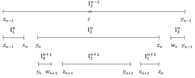
Figure 1: Intervals of next generations

From Figure 1, the end points of the intervals at each level are labeled by

$$z_{0}=0,\;y_{0}=1,\;I_{2}^{0}=[0,1]$$

and for $n\geq 1$

$x_{n}=\partial I_{1}^{n}\backslash\partial I_{2}^{n-1}$

$y_{2n-1}=min\{\partial I_{2}^{2n-1}\}$

$y_{2n}=max\{\partial I_{2}^{2n}\}$

$z_{2n-1}=max\{\partial I_{2}^{2n-1}\}$

$z_{2n}=min\{\partial I_{2}^{2n}\}$

$w_{n}=\partial I_{3}^{n}\backslash\partial I_{2}^{n-1}.$

Definition 2.2.

For a given proper scaling data $s:\mathbb{N}\rightarrow T_{3},$ a map $f_{s}$ is said to be period tripling infinitely renormalizable if for $n\geq 1,$

• $[f_{s}(y_{n}),1]$ is the maximal domain containing $1$ on which $f_{s}^{3^{n}-1}$ is defined affinely and $[0,f_{s}^{2}(y_{n})]$ is the maximal domain containing $0$ on which $f_{s}^{3^{n}-2}$ is defined affinely,

• $f_{s}^{3^{n}-1}([f_{s}(y_{n}),1])=I_{2}^{n},$
  $f_{s}^{3^{n}-2}([0,f_{s}^{2}(y_{n})])=I_{2}^{n}.$

The combinatorics for period tripling renormalization is shown in Figure 2.

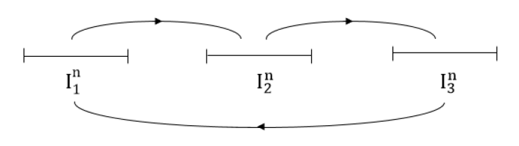
Figure 2: Period triple interval combinatorics ($I_{2}^{n}\rightarrow I_{3}^{n}\rightarrow I_{1}^{n}\rightarrow I_{2}^{n}).$

Let $U_{\infty}$ be the collection of period tripling infinitely renormalizable maps.
Let $f_{s}\in U_{\infty}$ be given by the proper scaling data $s:\mathbb{N}\rightarrow T_{3}$ and define

$${\tilde{I}}_{2}^{n}=[0,min\{u_{c}^{-1}(z_{n})\}]=[0,min\{f_{s}^{-1}(z_{n})\}],$$

where $u_{c}^{-1}(x)$ denotes the preimage(s) of $x$ under $u_{c}$ and

$${\hat{I}}_{2}^{n}=[u_{c}(y_{n}),1]=[f_{s}(y_{n}),1].$$

Let

$$h_{s,n}:[0,1]\rightarrow[0,1]$$

be defined by

$$h_{s,n}=\tilde{s}_{2}(1)\circ\tilde{s}_{2}(2)\circ\tilde{s}_{2}(3)\circ.....\circ\tilde{s}_{2}(n).$$

Furthermore, let

$${\tilde{h}}_{s,n}:[0,1]\rightarrow{\tilde{I}}_{2}^{n}\;\;\textrm{and}\;\;{\hat{h}}_{s,n}:[0,1]\rightarrow{\hat{I}}_{2}^{n}$$

be the affine orientation preserving homeomorphisms.

Then define

$$R_{n}f_{s}:h_{s,n}^{-1}(D_{s})\rightarrow[0,1]$$

by

$$R_{n}f_{s}(x)=\left\{\begin{array}[]{ll}R_{n}^{-}f_{s}(x),\;\;\;\;\;\textrm{if}\;x\in h_{s,n}^{-1}(I_{1}^{n})\\ R_{n}^{+}f_{s}(x),\;\;\;\;\;\textrm{if}\;x\in h_{s,n}^{-1}(I_{3}^{n})\end{array}\right.$$

where,

$$R_{n}^{-}f_{s}:h_{s,n}^{-1}(\mathop{\cup}\limits_{n\geq 1}I_{1}^{n})\rightarrow[0,1]$$

and

$$R_{n}^{+}f_{s}:h_{s,n}^{-1}(\mathop{\cup}\limits_{n\geq 1}I_{3}^{n})\rightarrow[0,1]$$

are defined by

$$R_{n}^{-}f_{s}(x)={\tilde{h}}_{s,n}^{-1}\circ f_{s}^{-1}\circ h_{s,n}(x)$$

$$R_{n}^{+}f_{s}(x)={\hat{h}}_{s,n}^{-1}\circ f_{s}\circ h_{s,n}(x),$$

which are illustrated in Figure 3.

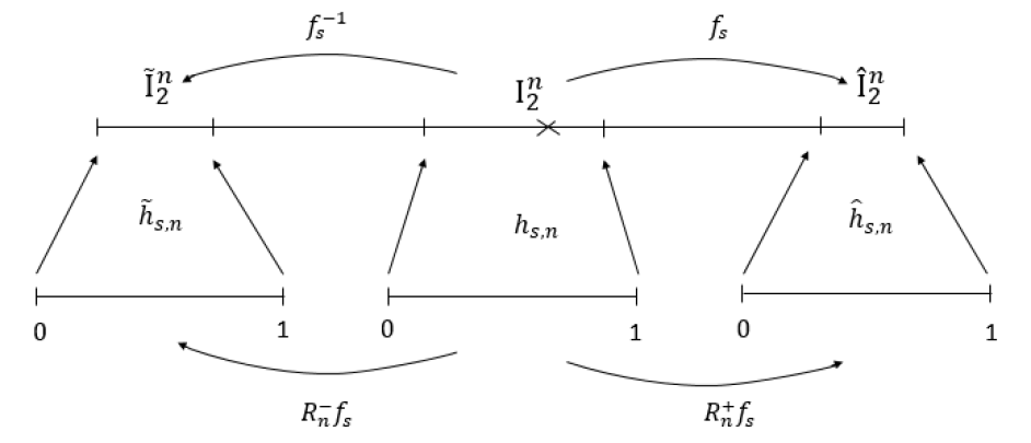
Figure 3:

Let $\sigma:T_{k}^{\mathbb{N}}\rightarrow T_{k}^{\mathbb{N}}$ be the shift map $\sigma(s)(n)=s(n+1).$ The above construction gives us the following result,

Lemma 2.1.

Let $s:\mathbb{N}\rightarrow T_{3}$ be proper scaling data such that $f_{s}$ is infinitely renormalizable. Then

$$R_{n}{f_{s}}=f_{\sigma^{n}(s)}.$$

Let $f_{s}$ be infinitely renormalization, then for $n\geq 0,$ we have

$$f_{s}^{3^{n}}:D_{s}\cap I_{2}^{n}\rightarrow I_{2}^{n}$$

is well defined.
 Now we define the renormalization $R:U_{\infty}\rightarrow U_{\infty}$ as

$$Rf_{s}=h_{s,1}^{-1}\circ f_{s}^{3}\circ h_{s,1}.$$

The maps $f_{s}^{3^{n}-2}:{\tilde{I}}_{2}^{n}\rightarrow I_{2}^{n}$ and $f_{s}^{3^{n}-1}:{\hat{I}}_{2}^{n}\rightarrow I_{2}^{n}$ are the affine homeomorphisms whenever $f_{s}\in U_{\infty}$. Then we have

Lemma 2.2.

$R^{n}{f_{s}}:D_{\sigma^{n}(s)}\rightarrow[0,1]$ and $R^{n}{f_{s}}=R_{n}{f_{s}}.$

The 2.1 and 2.2 give the following result.

Proposition 2.3.

There exists a map $f_{s^{*}}\in U_{\infty},$ where $s^{*}$ is characterized by

$$Rf_{s^{*}}=f_{s^{*}}.$$

In particular, $U_{\infty}=\{f_{s^{*}}\}.$

Proof.

Consider $s:\mathbb{N}\rightarrow T_{3}$ be proper scaling data such that $f_{s}$ is an infinitely renormalizable. Let $c_{n}$ be the critical point of $f_{\sigma^{n}(s)}.$ Then

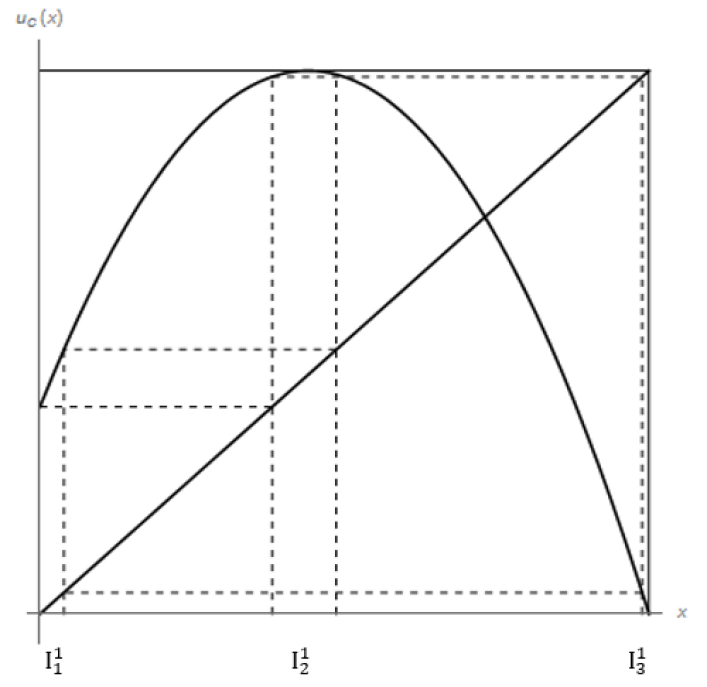
Figure 4: Period three cobweb diagram

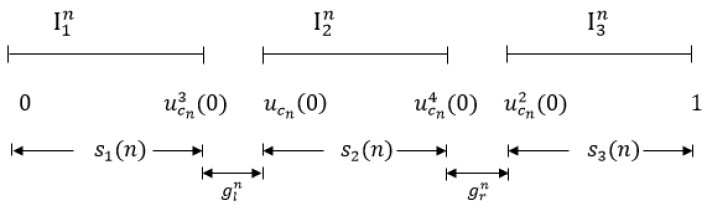
Figure 5: Length of the intervals gaps

from Figures 4 and 5, we have the following

$$u_{c_{n}}^{2}(0) =1-s_{3}(n)$$ (2.1)

$$u_{c_{n}}^{3}(0) =u_{c_{n}}(1-s_{3}(n))$$ (2.2)

$$=s_{1}(n)$$

$$u_{c_{n}}^{4}(0) =s_{2}(n)+u_{c_{n}}(0)$$ (2.3)

$$c_{n+1} =\frac{u_{c_{n}}^{4}(0)-c_{n}}{s_{2}(n)}.$$ (2.4)

Since $(s_{1}(n),s_{2}(n),s_{3}(n))\in T_{3},$ we have the following conditions

$$s_{i}(n)>0,\;\textrm{for}\;i=1,2,3$$ (2.5)

$$s_{1}(n)+s_{2}(n)+s_{3}(n) <1$$ (2.6)

As the intervals $I_{i}^{n},$ for $i=1,2,3,$ are pairwise disjoint, let $g_{l}^{n}$ and $g_{r}^{n}$ are the gaps between $I_{1}^{n}\;\&\;I_{2}^{n}$ and $I_{2}^{n}\;\&\;I_{3}^{n}$ respectively, which are shown in Figure 5. Then we have, for $n\in\mathbb{N},$

$$g_{l}^{n}=u_{c_{n}}(0)-u_{c_{n}}^{3}(0)\equiv G_{l}(c_{n})>0$$ (2.7)

$$g_{r}^{n}=u_{c_{n}}^{2}(0)-u_{c_{n}}^{4}(0)\equiv G_{r}(c_{n})>0$$ (2.8)

$$0<c_{n}<\frac{1}{2}$$ (2.9)

Solving Eqns. (2.1), (2.2), (2.3) and (2.4) by using Mathematica, we get

$$s_{1}(n)=1-\frac{(c_{n}-8c_{n}^{2}+21c_{n}^{3}-25c_{n}^{4}+17c_{n}^{5}-6c_{n}^{6}+c_{n}^{7})^{2}}{(1-c_{n})^{14}}\equiv S_{1}(c_{n})$$ (2.10)

$$s_{2}(n)=\frac{c_{n}^{2}(1-c_{n})^{28}-\Big{(}(-1+c_{n})^{15}+(c_{n}-8c_{n}^{2}+21c_{n}^{3}-25c_{n}^{4}+17c_{n}^{5}-6c_{n}^{6}+c_{n}^{7})^{2}\Big{)}^{2}}{(1-c_{n})^{30}}$$

$$\equiv S_{2}(c_{n})$$ (2.11)

$$s_{3}(n)=\frac{(-1+3c_{n}-2c_{n}^{2}+c_{n}^{3})^{2}}{(1-c_{n})^{6}}\equiv S_{3}(c_{n})$$ (2.12)

$$c_{n+1}=\frac{(1-c_{n})^{31}-((1-c_{n})^{15}-(c_{n}-8c_{n}^{2}+21c_{n}^{3}-25c_{n}^{4}+17c_{n}^{5}-6c_{n}^{6}+c_{n}^{7})^{2})^{2}}{c_{n}^{2}(1-c_{n})^{28}-((1-c_{n})^{15}-(c_{n}-8c_{n}^{2}+21c_{n}^{3}-25c_{n}^{4}+17c_{n}^{5}-6c_{n}^{6}+c_{n}^{7})^{2})^{2}}$$

$$\equiv\mathcal{R}(c_{n})$$ (2.13)

The graphs of $S_{1},\;S_{2},\;S_{3}$ and $S_{1}+S_{2}+S_{3}$ are shown in Figures 6 and 7.

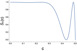
(a)

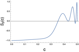
(b)

Figure 6: (6(a)) and (6(b)) show the graphs of $S_{1}(c)$ and $S_{2}(c)$ respectively.

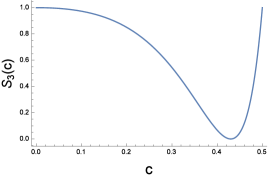
(a)

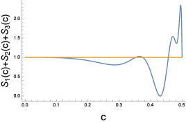
(b)

Figure 7: (7(a)) and (7(b)) show the graphs of $S_{3}(c)$ and $(S_{1}+S_{2}+S_{3})(c)$ respectively.

Note that the conditions (2.5). (2.7) and (2.8) gives the condition (2.6)

$$0<\sum_{i=1}^{3}s_{i}(n)<1.$$

Therefore, the condition (2.5) together with (2.7), (2.8) and (2.9) define the feasible domain $F_{d}$ to be:

$$F_{d}=\Big{\{}\;c\in\left(0,\;\frac{1}{2}\right)\;:\;S_{i}(c)>0\;\textrm{for}\;i=1,2,3,\;G_{l}(c)>0,\;G_{r}(c)>0\Big{\}}$$ (2.14)

To compute the feasible domain $F_{d},$ we need to find subinterval(s) of $(0,0.5)$ which satisfies the conditions of (2.14). By using Mathematica software, we employ the following command to obtain the feasible domain

$$\textup{N[Reduce[$\{S_{1}(c)>0,S_{2}(c)>0,S_{3}(c)>0,G_{l}(c)>0,G_{r}(c)>0,0<c<0.5\}$,c]]}.$$

This yields:

$$F_{d}=(0.398039...,\;0.430159...)\cup(0.430159...,\;0.456310...)\equiv F_{d_{1}}\cup F_{d_{2}}.$$

From the Eqn.(2.13), the graphs of $\mathcal{R}(c)$ are plotted in the sub-domains $F_{d_{1}}$ and $F_{d_{2}}$ of $F_{d}$ which are shown in Figure 8.

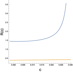
(a) $\mathcal{R}$ has no fixed point in $F_{d_{1}}.$

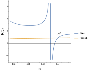
(b) $\mathcal{R}$ has only one fixed point in $F_{d_{2}}.$

Figure 8: The graph of $\mathcal{R}:F_{d}\rightarrow\mathbb{R}$ and the diagonal $\mathcal{R}(c)=c.$

Clearly, the map $\mathcal{R}:F_{d}\rightarrow\mathbb{R}$ is expanding in the neighborhood of the fixed point $c^{*}$ which is shown in Figure 8(b). By using Mathematica, we compute the only fixed point $c^{*}=0.440262...$ in $F_{d}$ such that

$$\mathcal{R}(c^{*})=c^{*}$$

corresponds to the infinitely renormalizable map $f_{s^{*}}.$

The graphs of piece-wise infinitely renormalizable map $f_{s^{*}}$ and zoomed part of $f_{s^{*}}$ are shown in the Figure 9.

(a) $f_{s^{*}}$ in $[0,1].$

(b) Zoomed part of $f_{s^{*}}$ in $[0.4396,0.4408]$

Figure 9: The graph of map $f_{s^{*}}.$

In other words, consider the scaling data $s^{*}:\mathbb{N}\rightarrow T_{3},$ with

$$s^{*}(n) =(s_{1}^{*}(n),\;s_{2}^{*}(n),\;s_{3}^{*}(n))$$

$$=(u_{c^{*}}^{3}(0),\;u_{c^{*}}^{4}(0)-u_{c^{*}}(0),\;1-u_{c^{*}}^{2}(0)).$$

Then $\sigma(s^{*})=s^{*}$ and using Lemma 2.1 we have

$$Rf_{s^{*}}=f_{s^{*}}.$$

∎

Lemma 2.4.

If $f_{{s}^{*}}$ is the map with a proper scaling data ${s}^{*}=(s_{1}^{*},s_{2}^{*},s_{3}^{*}),$ then we have

$$(s_{2}^{*})^{2}=s_{3}^{*}.$$

Proof.

Let $\hat{I}_{2}^{n}=f_{{s}^{*}}(I_{2}^{n})=[f_{{s}^{*}}(y_{n}),1]$ and $\hat{I}_{3}^{n+1}=f_{{s}^{*}}(I_{3}^{n+1}).$ Then $f_{{s}^{*}}^{3^{n}-1}:\hat{I}_{2}^{n}\rightarrow I_{2}^{n}$ is affine, monotone and onto. Further, by construction

$$f_{{s}^{*}}^{3^{n}-1}:\hat{I}_{2}^{n+1}\rightarrow I_{3}^{n+1}.$$

Hence,

$$\frac{|\hat{I}_{2}^{n+1}|}{|\hat{I}_{2}^{n}|}=s_{3}^{*}.$$

Therefore, $|I_{2}^{n}|=(s_{2}^{*})^{n}$ and $|\hat{I}_{2}^{n}|=(s_{3}^{*})^{n}$. Since,

$$f_{{s}^{*}}(y_{n})=u_{{c}^{*}}(y_{n}).$$

This implies,

$$s_{3}^{*}=\frac{|\hat{I}_{2}^{n+1}|}{|\hat{I}_{2}^{n}|}=\left(\frac{{y_{n+1}}-c}{{y_{n}}-c}\right)^{2}=\left(\frac{|{I}_{2}^{n+1}|}{|{I}_{2}^{n}|}\right)^{2}=(s_{2}^{*})^{2}.$$

∎

Remark 1.

A proper scaling data $(s_{1}^{*},s_{2}^{*},s_{3}^{*})$ is satisfying the following properties, for all $n\in\mathbb{N},$

1. $\frac{|I_{2}^{n+1}|}{|I_{2}^{n}|}=s_{2}^{*}$ and $\frac{|I_{1}^{n+1}|}{|I_{1}^{n}|}=\frac{|I_{3}^{n+1}|}{|I_{3}^{n}|}=s_{2}^{*}$

2. $\frac{|I_{1}^{n+1}|}{|I_{2}^{n}|}=s_{1}^{*}$

3. $\frac{|I_{3}^{n+1}|}{|I_{2}^{n}|}=s_{3}^{*}$

Remark 2.

Let $I_{2}^{n}=[y_{n},z_{n}]$ be the interval containing $c^{*}$ corresponding to the scaling data $s^{*}=(s_{1}^{*},s_{2}^{*},s_{3}^{*})$ then

$$f_{s^{*}}(y_{n})=u_{c^{*}}(y_{n}).$$

Hence, $f_{s^{*}}$ has a quadratic tip.

Remark 3.

The invariant Cantor set of the map $f_{s^{*}}$ is more complex than the invariant period doubling Cantor set of piece-wise affine infitely renormalizable map [8]. The complexity in the sense that:

• The geometry of Cantor set of $f_{s^{*}}$ is similar to the geometry of Cantor set of [8], on each scale and everywhere the same scaling ratios are used,

• But unlike the Cantor set of [8], there are now three ratios at each scale.

Furthermore, the scaling data corresponding to $f_{s^{*}}$ is very different from the geometry of Cantor attractor of analytic renormalization fixed point, in which there are no two places where the same scaling ratios are used at all scales and where the closure of the set of ratios itself a Cantor set [9] .

2.2 $C^{1+Lip}$ extension of $f_{s^{*}}$

In subsection 2.1, we constructed a piece-wise affine infinitely renormalizable map $f_{s^{*}}$ corresponding to the proper scaling data $s^{*}.$
Our goal is to construct an extension of $f_{s^{*}}$ in the class $C^{1+Lip}$, consisting of infinitely renormalizable maps.

Let $F:[0,1]^{2}\rightarrow[0,1]^{2}$ be the scaling function defined as

$$F\left(\begin{array}[]{ll}x\\ y\end{array}\right)=\left(\begin{array}[]{ll}u_{c^{*}}(0)+s_{2}^{*}(1-x)\\ 1-s_{3}^{*}(1-y)\end{array}\right)\equiv\left(\begin{array}[]{ll}F_{1}(x)\\ F_{2}(y)\end{array}\right)$$

Let $K$ be the graph of $\mathcal{F}_{s^{*}}$ which is an extension of $f_{s^{*}},$ where $f_{s^{*}}:D_{s^{*}}\rightarrow[0,1].$ Let $K^{1}$ and $K^{2}$ be the graph of $\mathcal{F}_{s^{*}}|_{[z_{1},y_{0}]}$ and $\mathcal{F}_{s^{*}}|_{[z_{0},y_{1}]},$ respectively, as shown in Figure 10. Then

$$K=\cup_{m\geq 1}F^{m}(K^{1}\cup K^{2})$$

is the graph of $\mathcal{F}_{s^{*}}.$ We claim that $\mathcal{F}_{s^{*}}$ is a $C^{1+Lip}$ unimodal map with quadratic tip.

Let $B_{0}=[0,1]\times[0,1]$ and for each $n\in\mathbb{N},\textrm{define}$ $B_{n}=F^{n}(B_{0})$ as:

$B_{n}=\left\{\begin{array}[]{ll}\;[y_{n},z_{n}]\times[\tilde{y}_{n},1],\;\;\;\textrm{if}\;n\;\textrm{is odd}\\ \ [z_{n},y_{n}]\times[\tilde{y}_{n},1],\;\;\;\textrm{if}\;n\;\textrm{is even}\end{array}\right.$

Also, let $p_{n}$ be the point on the graph of the unimodal map $u_{{c}^{*}}(x).$ For all $n\in\mathbb{N},$ define

$p_{n}=\left\{\begin{array}[]{ll}(y_{\frac{n+1}{2}},\tilde{y}_{\frac{n+1}{2}}),\;\;\;\textrm{if}\;n\;\textrm{is odd}\\ (z_{\frac{n}{2}},\tilde{z}_{\frac{n}{2}}),\;\;\;\;\;\;\;\;\;\textrm{if}\;n\;\textrm{is even}\end{array}\right.$
where $\tilde{y}_{n}=u_{c^{*}}(y_{n})$ and $\tilde{z}_{n}=u_{c^{*}}(z_{n}).$

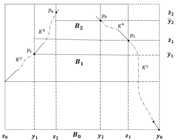
Figure 10: Extension of $f_{s^{*}}$

Then the above construction of boxes $B_{n}$ together with the points $p_{n}$ will lead to following proposition,

Proposition 2.5.

$K$ is the graph of $\mathcal{F}_{s^{*}}$ which is a $C^{1}$ extension of $f_{s^{*}}.$

Proof.

Since $K^{1}$ and $K^{2}$ are the graph of $f_{s^{*}}|_{[z_{1},y_{0}]}$ and $f_{s^{*}}|_{[z_{0},y_{1}]},$ respectively, we obtain $K^{2n+1}=F^{n}(K^{1})$ and $K^{2n+2}=F^{n}(K^{2})$ for each $n\in\mathbb{N}.$
Note that $K^{n}$ is the graph of a $C^{1}$ function defined

on $$[y_{\frac{n-1}{2}},\;z_{\frac{n+1}{2}}]\;\;\;\textrm{if}\;\;n\in 4\mathbb{N}-1,$$

on $$[y_{\frac{n}{2}},\;z_{\frac{n}{2}-1}]\;\;\;\;\;\textrm{if}\;\;n\in 4\mathbb{N},$$

on $$[z_{\frac{n+1}{2}},\;y_{\frac{n-1}{2}}]\;\;\;\textrm{if}\;\;n\in 4\mathbb{N}+1,$$

and on $$[z_{\frac{n}{2}-1},\;y_{\frac{n}{2}}]\;\;\;\;\;\textrm{if}\;\;n\in 4\mathbb{N}+2.$$

To prove the proposition, we have to check continuous differentiability at the points $p_{n}.$ Consider a neighborhoods $(y_{1}-\epsilon,y_{1}+\epsilon)$ around $y_{1}$ and $(z_{1}-\epsilon,z_{1}+\epsilon)$ around $z_{1}$, the slopes are given by an affine pieces of $f_{s^{*}}$ on the subintervals $(y_{1},y_{1}+\epsilon)$ and $(z_{1}-\epsilon,z_{1})$ and the slopes are given by the chosen $C^{1}$ extension on $(y_{1}-\epsilon,y_{1})$ and $(z_{1},z_{1}+\epsilon).$ This implies, $K^{1}$ and $K^{2}$ are $C^{1}$ at $p_{2}$ and $p_{1},$ respectively.
Let $\Upsilon_{1}\subset K$ be the graph over the interval $(z_{1}-\epsilon,z_{1}+\epsilon)$ and $\Upsilon_{2}\subset K$ be the graph over the interval $(y_{1}-\epsilon,y_{1}+\epsilon),$
then the graph $K$ locally around $p_{n}$ is equal to $\left\{\begin{array}[]{ll}F^{\frac{n-1}{2}}{(\Upsilon_{2})}\;\;\;\textrm{if}\;n\;\textrm{is odd}\\ F^{\frac{n-2}{2}}{(\Upsilon_{1})}\;\;\;\textrm{if}\;n\;\textrm{is even}\end{array}\right.$.
This implies, for $n\in\mathbb{N},$ $K^{2n-1}$ is $C^{1}$ at $p_{2n}$ and $K^{2n}$ is $C^{1}$ at $p_{2n-1}.$
Hence $K$ is a graph of a $C^{1}$ function on $[0,1]\setminus\{c^{*}\}.$
From Lemma 2.4, we observe that the horizontal contraction of $F$ is smaller than the vertical contraction. This implies that the slope of $K^{n}$ tends to zero when $n$ is large.
Therefore, $K$ is the graph of a $C^{1}$ function on $[0,1].$ ∎

Proposition 2.6.

Let $\mathcal{F}_{s^{*}}$ be the function whose graph is $K$ then $\mathcal{F}_{s^{*}}$ is a $C^{1+Lip}$ map with a quadratic tip.

Proof.

As the function $\mathcal{F}_{s^{*}}$ is a $C^{1}$ extension of $f_{s^{*}}$ and $\left.f_{s^{*}}\right|_{D_{s}}$ has a quadratic tip, therefore $\mathcal{F}_{s^{*}}$ has a quadratic tip. We have to show that $K^{n}$ is the graph of a $C^{1+Lip}$ function

$$\mathcal{F}_{s^{*}}^{n}:Dom(K^{n})\rightarrow[0,1]$$

with an uniform Lipschitz bound.
That is, for $n\geq 1,$

$$Lip((\mathcal{F}_{s^{*}}^{n+1})^{\prime})\leq Lip((\mathcal{F}_{s^{*}}^{n})^{\prime})$$

Let us assume that $\mathcal{F}_{s^{*}}^{n}$ is $C^{1+Lip}$ with Lipschitz constant $\lambda_{n}$ for its derivatives. We show that $\lambda_{n+1}\leq\lambda_{n}$.
For given $(a,b)$ on the graph of $\mathcal{F}_{s^{*}}^{n},$ there is $(\bar{a},\bar{b})=F(a,b)$ on the graph of $\mathcal{F}_{s^{*}}^{n+1}$, this implies

$$\mathcal{F}_{s^{*}}^{n+1}(\bar{a})=1-s_{3}^{*}+s_{3}^{*}\cdot\mathcal{F}_{s^{*}}^{n}(a)$$

Since $a=1-\frac{\bar{a}-u_{c^{*}}(0)}{{s_{2}^{*}}},$ we have

$$\mathcal{F}_{s^{*}}^{n+1}(\bar{a})=1-s_{3}^{*}+s_{3}^{*}\cdot\mathcal{F}_{s^{*}}^{n}\left(1-\frac{\bar{a}-u_{c^{*}}(0)}{{s_{2}^{*}}}\right)$$

Differentiate both sides with respect to $\bar{a}$, we get

$$(\mathcal{F}_{s^{*}}^{n+1})^{\prime}(\bar{a})=\frac{-s_{3}^{*}}{{s_{2}^{*}}}(\mathcal{F}_{s^{*}}^{n})^{\prime}\left(1-\frac{\bar{a}-u_{c^{*}}(0)}{{s_{2}^{*}}}\right)$$

Therefore,

$$|(\mathcal{F}_{s^{*}}^{n+1})^{\prime}(\bar{a}_{1})-(\mathcal{F}_{s^{*}}^{n+1})^{\prime}(\bar{a}_{2})| =\bigg{|}\frac{-s_{3}^{*}}{{s_{2}^{*}}}\bigg{|}\cdot\bigg{|}(\mathcal{F}_{s^{*}}^{n})^{\prime}\left(1-\frac{\bar{a}_{1}-u_{c^{*}}(0)}{{s_{2}^{*}}}\right)-(\mathcal{F}_{s^{*}}^{n})^{\prime}\left(1-\frac{\bar{a}_{2}-u_{c^{*}}(0)}{{s_{2}^{*}}}\right)\bigg{|}$$ (2.15)

$$\leq\frac{s_{3}^{*}}{({s_{2}^{*}})^{2}}\cdot\lambda(\mathcal{F}_{s^{*}}^{n})^{\prime}|\bar{a}_{1}-\bar{a}_{2}|$$

From Lemma 2.4, we have $({s_{2}^{*}})^{2}={s_{3}^{*}}.$ Therefore,

$$\lambda(\mathcal{F}_{s^{*}}^{n+1})^{\prime}\leq\lambda(\mathcal{F}_{s^{*}}^{n})^{\prime}\leq\lambda(\mathcal{F}_{s^{*}}^{1})^{\prime}$$

This completes the proof. ∎

Note that $f_{s^{*}}$ is infinitely renormalizable piece-wise affine map and $\mathcal{F}_{s^{*}}$ is the $C^{1+Lip}$ extension of $f_{s^{*}}$ which is not a $C^{2}$ map . Then it implies that $\mathcal{F}_{s^{*}}$ is renormalizable. We observe that $R\mathcal{F}_{s^{*}}$ is an extension of $Rf_{s^{*}}.$ Therefore $R\mathcal{F}_{s^{*}}$ is renormalizable. Hence, $\mathcal{F}_{s^{*}}$ is infinitely renormalizable map. Then we have the following theorem,

Theorem 2.7.

There exists a period tripling infinitely renormalizable $C^{1+Lip}$ unimodal map $\mathcal{F}_{s^{*}}$ with a quadratic tip such that

$$R\mathcal{F}_{s^{*}}=\mathcal{F}_{s^{*}}.$$

2.3 Topological entropy of renormalization

In this section, we calculate the topological entropy of period tripling renormalization operator.
Let us consider three $C^{1+Lip}$ maps $\psi_{0}:[0,y_{1}]\cup[z_{1},1]\rightarrow[0,1],$ $\psi_{1}:[0,y_{1}]\cup[z_{1},1]\rightarrow[0,1],$ and $\psi_{2}:[0,y_{1}]\cup[z_{1},1]\rightarrow[0,1]$ which extend $f_{s^{*}}.$ For a sequence $\alpha=\{\alpha_{n}\}_{n\geq 1}\in\Sigma_{3},$
where $\Sigma_{3}=\{\{x_{n}\}_{n\geq 1}:x_{n}\in\{0,\;1,\;2\}\}$ is called full 3-Shift.
Now define

$$K^{n}(\alpha)=F^{n}(graph\;\psi_{{\alpha}_{n}}),$$

we have

$$K(\alpha)=\bigcup\limits_{n\geq 1}K^{n}(\alpha).$$

Therefore, we conclude that $K(\alpha)$ is the graph of a $C^{1+Lip}$ map $f_{\alpha}$ having quadratic tip by using the same facts of subsection 2.2.
The shift map $\sigma:\Sigma_{3}\rightarrow\Sigma_{3}$ is defined as

$$\sigma(\alpha_{1}\alpha_{2}\alpha_{3}\ldots)=(\alpha_{2}\alpha_{3}\alpha_{4}\ldots).$$

Proposition 2.8.

The map $f_{\alpha}^{3}:[y_{1},\;z_{1}]\rightarrow[y_{1},\;z_{1}]$ is a unimodal map for all $\alpha\in\Sigma_{3}.$ Furthermore, $f_{\alpha}$ is period tripling renormalizable and $Rf_{\alpha}=f_{\sigma(\alpha)}.$

Proof.

We know that $f_{\alpha}:[y_{1},\;z_{1}]\rightarrow I_{3}^{1}$ is a unimodal and onto, $f_{\alpha}:I_{3}^{1}\rightarrow I_{1}^{1}$ is onto and affine and also $f_{\alpha}:I_{1}^{1}\rightarrow[y_{1},\;z_{1}]$ is onto and affine. Therefore $f_{\alpha}$ is renormalizable. The above construction implies

$$Rf_{\alpha}=f_{\sigma(\alpha)}.$$

∎

This gives us the following theorem.

Theorem 2.9.

The period tripling renormalization operator $R$ defined on the space of $C^{1+Lip}$ unimodal maps has positive topological entropy.

Proof.

From the above construction, we conclude that $\alpha\longmapsto f_{\alpha}\in C^{1+Lip}$ is injective. The domain of $R$ contains a subset $\Lambda$ on which $R$ is topological conjugate to the full 3-shift. As topological entropy $h_{top}$ is an invariant of topological conjugacy. Hence $h_{top}(\left.R\right|_{\Lambda})\geq\ln 3.$ ∎

In fact, the topological entropy of period tripling operator $R$ on $C^{1+Lip}$ unimodal maps is unbounded because if we choose $n$ different $C^{1+Lip}$ maps, say, $\psi_{0},\;\psi_{1},\;\psi_{2},\ldots\psi_{n-1},$ which extends $f_{s^{*}},$ then it will be embedded a full $n-\textrm{shift}$ in the domain of $R$.

2.4 An $\epsilon-$variation of the scaling data

In this section, we use an $\epsilon$ variation on the construction of scaling data as presented in subsection  2.1 to obtain the following theorem.

Theorem 2.10.

There exists a continuum of fixed points of period tripling renormalization operator acting on $C^{1+Lip}$ unimodal maps.

Proof.

Consider an $\epsilon$ variation on scaling data and we modify the construction which is described in subsection  2.1. This modification is illustrated in Figure 11.

Define a neighborhood $N_{\epsilon}$ about the point $(u_{c}^{2}(0),\;u_{c}^{3}(0))$ as

$$N_{\epsilon}(u_{c}^{2}(0),\;u_{c}^{3}(0))=\{(u_{c}^{2}(0),\;\epsilon\cdot u_{c}^{3}(0))\;:\;\epsilon>0\;\textrm{ and}\;\epsilon\;\textrm{close to }1\}.$$

Figure 11: $\epsilon$- perturbation of $s_{3}(c).$

From above Figure 11, the scaling data is obtained as

$$s_{3}(c,\epsilon) =1-u_{c}^{2}(0)$$

$$s_{1}(c,\epsilon) =\epsilon\cdot u_{c}^{3}(0)$$

$$s_{2}(c,\epsilon) =u_{c}(\epsilon\cdot u_{c}^{3}(0))-u_{c}(0)$$

where $c\in(0,\frac{1}{2}).$ Also, we define

$$\mathcal{R}(c,\epsilon) =\frac{u_{c}(\epsilon\cdot u_{c}^{3}(0))-c}{s_{2}(c,\epsilon)}.$$

From subsection 2.1, we know that the period tripling renormalization operator $\mathcal{R}$ has unique fixed point $c^{*}$. Consequently, for each $\epsilon,$ $\mathcal{R}(c,\epsilon)$ has only one unstable fixed point, namely $c_{\epsilon}^{*}.$ Therefore, we consider the perturbed scaling data ${s}_{\epsilon}^{*}:\mathbb{N}\rightarrow T_{3}$ with

$${s}_{\epsilon}^{*}(n)=(\epsilon\cdot u_{c_{\epsilon}^{*}}^{3}(0),\;u_{c_{\epsilon}}(\epsilon\cdot u_{c_{\epsilon}^{*}}^{3}(0))-u_{c_{\epsilon}^{*}}(0),\;1-u_{c_{\epsilon}^{*}}^{2}(0)).$$

Then $\sigma(s_{\epsilon}^{*})={s}_{\epsilon}^{*}$ and using Lemma 2.1, we have

$$Rf_{{s}_{\epsilon}^{*}}=f_{{s}_{\epsilon}^{*}}.$$

Moreover, $f_{{s}_{\epsilon}^{*}}$ is a piece-wise affine map which is infinitely renormalizable. Now we use similar extension described in subsection 2.2, then we get $\mathcal{F}_{{s}_{\epsilon}^{*}}$ is the $C^{1+Lip}$ extension of $f_{{s}_{\epsilon}^{*}}$. This implies that $\mathcal{F}_{{s}_{\epsilon}^{*}}$ is a renormalizable map. As $R\mathcal{F}_{{s}_{\epsilon}^{*}}$ is an extension of $Rf_{{s}_{\epsilon}^{*}}.$ Therefore $R\mathcal{F}_{{s}_{\epsilon}^{*}}$ is renormalizable. Hence, for each $\epsilon$ close to $1,$ $\mathcal{F}_{{s}_{\epsilon}^{*}}$ is a fixed point of period tripling renormalization. This proves the existence of a continuum of fixed points of renormalization. ∎

Remark 4.

• When $\epsilon=1,$ the fixed point of $\mathcal{R}(c,\epsilon)$ coincides with the fixed point of $\mathcal{R}(c)$ which is described in subsection 2.1.

• On the other hand, we have the following relations

  • if $\epsilon<1,$ then

    $$c^{*}<c_{\epsilon}^{*},$$

  • if $\epsilon>1,$ then

    $$c_{\epsilon}^{*}<c^{*},$$

  • if $\epsilon_{0}<\epsilon_{1},$ then

    $$c_{\epsilon_{1}}^{*}<c_{\epsilon_{0}}^{*},$$

The above relations $(i)$ and $(ii)$ are illustrated in Figure 12 by plotting the graphs of $\mathcal{R}(c,\epsilon)$ as a thick line and $\mathcal{R}(c)$ as a dotted line.

(a)

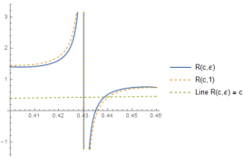
(b)

Figure 12: (12(a)): $\mathcal{R}(c,\epsilon)$ and $\mathcal{R}(c)$ for $\epsilon<1$ and (12(b)): $\mathcal{R}(c,\epsilon)$ and $\mathcal{R}(c)$ for $\epsilon>1.$

Lemma 2.11.

There exists $\rho>0$ such that

$$\frac{1}{\rho}\leq\frac{|\hat{I}_{2}^{n}|}{|I_{2}^{n}|^{2}}\leq\rho.$$

Proof.

We have

$I_{2}^{n}=\left\{\begin{array}[]{ll}\;[y_{n},z_{n}],\;\;\;\textrm{for}\;\;n=1,3,5,...\\ \ [z_{n},y_{n}],\;\;\;\textrm{for}\;\;n=2,4,6,...\end{array}\right.$

and

$I_{3}^{n}=\left\{\begin{array}[]{ll}\;[w_{n},y_{n-1}],\;\;\;\textrm{for}\;\;n=1,3,5,...\\ \ [y_{n-1},w_{n}],\;\;\;\textrm{for}\;\;n=2,4,6,...\end{array}\right.$

where $y_{n}$ $z_{n}$ and $w_{n}$ are defined in subsection 2.1.

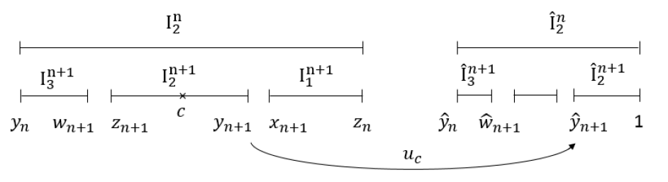
Figure 13:

Let

$$\hat{I}_{2}^{n}=u_{c}({I}_{2}^{n})=[u_{c}(y_{n}),1]=[\hat{y}_{n},1].$$

and

$$\hat{I}_{3}^{n}=[\hat{y}_{n},\hat{w}_{n+1}]\subset\hat{I}_{2}^{n}$$

such that

$$|\hat{I}_{3}^{n+1}|=s_{2}(n)|\hat{I}_{2}^{n}|.$$

Define an affine homeomorphism $f_{\alpha}:{I}_{3}^{n+1}\rightarrow\hat{I}_{3}^{n+1}$ such that

$$f_{\alpha}(y_{n})=u_{c}(y_{n})=\hat{y}_{n}.$$

Also, we have $c(n)=c(\sigma^{n}\alpha)\in[c_{0}^{*},c_{2}^{*}]$ which is a small neighborhood of $c^{*}.$ This implies, there exists $\rho_{0}>0$ such that

$$\frac{1}{\rho_{0}}\leq\frac{|c-y_{n}|}{|I_{2}^{n}|}\leq\rho_{0}.$$ (2.16)

Then

$$\frac{|\hat{I}_{2}^{n}|}{|I_{2}^{n}|^{2}}=\frac{|[u_{c}(y_{n}),1]|}{|I_{2}^{n}|^{2}}=\frac{1}{|I_{2}^{n}|^{2}}\frac{(y_{n}-c)^{2}}{(1-c)^{2}}$$ (2.17)

From Eqns. (2.16) and (2.17), we have

$$\frac{1}{\rho_{0}^{2}(1-c)^{2}}\leq\frac{|\hat{I}_{2}^{n}|}{|I_{2}^{n}|^{2}}\leq\frac{\rho_{0}^{2}}{(1-c)^{2}}.$$

Since $(1-c)^{2}\leq\frac{1}{(1-c)^{2}}$, choose $\rho=\frac{\rho_{0}^{2}}{(1-c)^{2}}.$ Then we have

$$\frac{1}{\rho}\leq\frac{|\hat{I}_{2}^{n}|}{|I_{2}^{n}|^{2}}\leq\rho.$$

∎

Theorem 2.12.

There exists an infinitely renormalizable $C^{1+Lip}$ unimodal map $k$ with quadratic tip such that $\{c_{n}\}_{n\geq 0},$ where $c_{n}$ is the critical point of $R^{n}k,$ is dense in a Cantor set.

Proof.

From subsection 2.1, we conclude that the map $R$ has one fixed point $c^{*}$ which is expanding. We choose $\epsilon_{0}>\epsilon_{1}>\epsilon_{2}$ close to $1.$ Then $R(c,\epsilon_{0}),$ $R(c,\epsilon_{1})$ and $R(c,\epsilon_{2})$ have the expanding fixed points $c_{0}^{*},$ $c_{1}^{*}$ and $c_{2}^{*},$ respectively. In fact,

$$\frac{\partial R}{\partial c}(c_{i}^{*},\epsilon_{i})>2,\;\;\;\textrm{for each}\;i\;=\;0,\;1,\;2.$$

From Remark 4$(iii)$, we have $c_{0}^{*}<c_{1}^{*},<c_{2}^{*}.$ Therefore, there exists three intervals $A_{0}=[c_{0}^{*},\;a_{0}],$ $A_{1}=[a_{1},\;b_{1}]$ and $A_{2}=[a_{2},\;c_{2}^{*}],$ such that the maps

$$R_{i}:A_{i}\rightarrow[c_{0}^{*},\;c_{2}^{*}]\supset A_{i},\;\;\;\;\textrm{for}\;i=0,1,2,$$

are expanding diffeomorphisms, where $R_{i}(c)=R(c,\epsilon_{i}).$ Therefore, we get a horseshoe map. We use the following coding for the invariant Cantor set of the horseshoe map

$$c:\Sigma_{3}\rightarrow[c_{0}^{*},c_{2}^{*}]$$

with

$$c\left(\sigma(\alpha)\right)=\mathcal{R}\left(c(\alpha),\epsilon_{\alpha_{0}}\right).$$

Given a sequence $\alpha\in\Sigma_{3},$ the proper scaling data $s:\mathbb{N}\rightarrow\Delta^{3}$ is defined as

$$s(n)=\left(s_{1}(c(\sigma^{n}\alpha),\epsilon_{\alpha_{n}}),\;s_{2}(c(\sigma^{n}\alpha),\epsilon_{\alpha_{n}}),\;s_{3}(c(\sigma^{n}\alpha),\epsilon_{\alpha_{n}})\right).$$

Consequently, we define a piece-wise affine map

$$f_{\alpha}:D_{s}\rightarrow[0,1].$$

Define $F^{n}:[0,1]^{2}\rightarrow[0,1]^{2}$ by

$$F^{n}\left(\begin{array}[]{ll}x\\ y\end{array}\right)=\left(\begin{array}[]{ll}F_{1}^{n}(x)\\ F_{2}^{n}(y)\end{array}\right)$$

where $F_{2}^{n}$ be the affine orientation preserving homeomorphism and $F_{1}^{n}$ be the affine homeomorphism with $F_{1}^{n}(1)=y_{n}.$ Therefore, the image of $F^{n}$ is $B_{n}.$

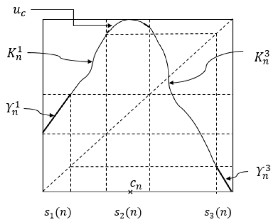
Figure 14:

Let $K^{n}=(F^{n})^{-1}(graph\;f_{\alpha})=\gamma_{n}^{1}\cup\gamma_{n}^{3}.$ This is the graph of $f_{\alpha_{n}}.$ We extend the function $f_{\alpha_{n}}$ and its graph $F_{n}$ on the gaps $[u_{c_{n}}^{3}(z_{n-1}),u_{c_{n}}(z_{n-1})]$ and $[u_{c_{n}}^{4}(z_{n-1}),u_{c_{n}}^{2}(z_{n-1})].$ Obverse that $u_{c_{n}}^{i}(z_{n-1})$ and $Df_{\alpha_{n}}(u_{c_{n}}^{i}(z_{n-1}))$ vary within a compact family. This allows us to choose from a compact family of $C^{1+Lip}$ diffeomorphisms the extensions

$$k_{n}^{1}:[z_{n-1},u_{c_{n}}(z_{n-1})]\rightarrow[f_{\alpha_{n}}(z_{n-1}),f_{\alpha_{n}}(u_{c_{n}}(z_{n-1}))]$$

and

$$k_{n}^{3}:[u_{c_{n}}^{4}(z_{n-1}),1]\rightarrow[0,f_{\alpha_{n}}(u_{c_{n}}^{4}(z_{n-1}))]$$

of the maps $f_{\alpha_{n}}$ on $I_{1}^{n}$ and $I_{3}^{n},$ respectively. Let $K_{n}^{1}$ and $K_{n}^{3}$ are the graphs of $k_{n}^{1}$ and $k_{n}^{3},$ respectively. Therefore,

$$K=\bigcup\limits_{n\geq 0}F^{n}(K_{n}^{1}\cup K_{n}^{3}).$$

Then $K$ is the graph of a unimodal map $k:[0,1]\rightarrow[0,1]$ which extends $f_{\alpha}.$ Notice that $k$ is $C^{1}.$ Since $f_{\alpha}$ has a quadratic tip, $k$ also has a quadratic tip. Also, $F^{n}(K^{n})$ is the graph of a $C^{1+Lip}$ diffeomorphism. For a similar reason as of Eqn. (2.15) in subsection 2.2, the Lipschitz bound $\lambda$ satisfies

$$\lambda_{n}\leq\frac{|\hat{I}_{2}^{n}|}{|I_{2}^{n}|^{2}}P_{0}\;\;\textrm{for some}\;\;P_{0}>0.$$

Using Lemma 2.11, we get

$$\lambda\leq P_{0}\cdot\rho.$$

Thus $k_{\alpha}$ is a $C^{1+Lip}$ unimodal map with quadratic tip. The construction implies that $k$ is infinitely renormalization and

$$graph(R^{n}k_{\alpha})\supset K^{n}.$$

By choosing $\alpha\in\Sigma_{3}$ such that the orbit under the shift $\sigma$ is dense in the invariant Cantor set of the horseshoe map.

∎

3 Period quintupling renormalization

In this section, we describe the construction of period quintupling renormalizable fixed point on the space of piece-wise affine infinitely renormalizable maps. Further, we
describe the extension of piece-wise affine renormalizable map to a $C^{1+Lip}$ unimodal map. Then, we discuss the entropy of period quintupling renormalization operator acting on the same space.

Consider $T_{k}$ as defined in subsection 2.1, for $k=5,$ each element $(s_{1},s_{2},s_{3},s_{4},s_{5})$ is called a scaling quint-factor. Define affine maps $\tilde{s}_{1},$ $\tilde{s}_{2},$ $\tilde{s}_{3},$ $\tilde{s}_{4}$ and $\tilde{s}_{5}$ induced by a scaling quint-factor,

$$\tilde{s}_{i}:[0,1]\rightarrow[0,1]\;\;\;\textrm{for}\;i=1,2,\cdots,5,$$

defined by

$$\tilde{s}_{1}(t) =s_{1}(1-t)$$

$$\tilde{s}_{2}(t) =u_{c}^{3}(0)+s_{2}(1-t)$$

$$\tilde{s}_{3}(t) =u_{c}(0)+s_{3}(1-t)$$

$$\tilde{s}_{4}(t) =u_{c}^{2}(0)-s_{4}(1-t)$$

$$\tilde{s}_{5}(t) =1-s_{5}(1-t)$$

The scaling quint-factor $s(n)=(s_{1}(n),s_{2}(n),s_{3}(n)),s_{4}(n)),s_{5}(n))\in T_{5}$ induces a quintuplet of affine maps $(\tilde{s}_{1}(n),\tilde{s}_{2}(n),\tilde{s}_{3}(n),\tilde{s}_{4}(n),\tilde{s}_{5}(n))$.
For each $n\in\mathbb{N}$ and $i\in\{1,2,..,5\},$ we define the following intervals:

$$I_{i}^{n}=\tilde{s}_{2}(1)\circ\tilde{s}_{2}(2)\circ\tilde{s}_{2}(3)\circ.....\circ\tilde{s}_{2}(n-1)\circ\tilde{s}_{i}(n)([0,1]).$$

Given a proper scaling data, define

$$\{c\}=\bigcap\limits_{n\geq 1}I_{2}^{n}.$$

A proper scaling data $s:\mathbb{N}\rightarrow T_{5}$ induces the set $D_{s}=\bigcup\limits_{n\geq 1}(I_{1}^{n}\cup I_{3}^{n}\cup I_{4}^{n}\cup I_{5}^{n}).$ Consider a map

$$g_{s}:D_{s}\rightarrow[0,1]$$

such that $g_{s}|_{I_{i}^{n}}$ is the affine extensions of $u_{c}|_{\partial I_{i}^{n}},$ for each $i\in\{1,3,4,5\}.$

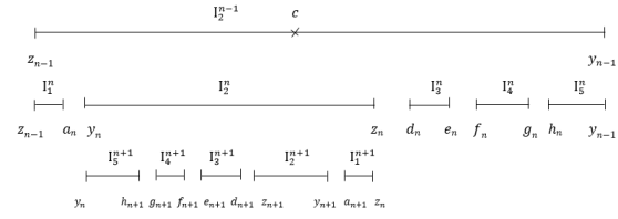
Figure 15: The intervals of next generations

From Figure 15, the end points of the intervals at each level are denoted by

$$z_{0}=0,\;y_{0}=1,\;I_{2}^{0}=[0,1]$$

and for $n\geq 1,$

$a_{n}=\partial I_{1}^{n}\backslash\partial I_{2}^{n-1}$

$y_{2n-1}=min\{\partial I_{2}^{2n-1}\},$          $y_{2n}=max\{\partial I_{2}^{2n}\}$

$z_{2n-1}=max\{\partial I_{2}^{2n-1}\},$          $z_{2n}=min\{\partial I_{2}^{2n}\}$

$d_{2n-1}=min\{\partial I_{3}^{2n-1}\},$          $d_{2n}=max\{\partial I_{3}^{2n}\}$

$e_{2n-1}=max\{\partial I_{3}^{2n-1}\},$          $e_{2n}=min\{\partial I_{3}^{2n}\}$

$f_{2n-1}=min\{\partial I_{4}^{2n-1}\},$          $f_{2n}=max\{\partial I_{4}^{2n}\}$

$g_{2n-1}=max\{\partial I_{4}^{2n-1}\},$          $g_{2n}=min\{\partial I_{4}^{2n}\}$

$h_{n}=\partial I_{5}^{n}\backslash\partial I_{2}^{n-1}$

Definition 3.1.

For a given proper scaling data $s:\mathbb{N}\rightarrow T_{5},$ a map $g_{s}$ is said to be period quintupling infinitely renormalizable if for $n\geq 1,$

• $[g_{s}(y_{n}),\;1]$ is the maximal domain containing $1$ on which $g_{s}^{5^{n}-1}$ is defined affinely and $[0,\;g_{s}^{2}(y_{n})]$ is the maximal domain containing $0$ on which $g_{s}^{5^{n}-2}$ is defined affinely,

• $[g_{s}(0),\;g_{s}^{3}(y_{n})]$ is the maximal domain on which $g_{s}^{5^{n}-3}$ is defined affinely and $[g_{s}^{4}(y_{n}),\;g_{s}^{2}(0)]$ is the maximal domain on which $g_{s}^{5^{n}-4}$ is defined affinely,

• $g_{s}^{5^{n}-1}([g_{s}(y_{n}),\;1])=I_{2}^{n},$
  $g_{s}^{5^{n}-2}([0,\;g_{s}^{2}(y_{n})])=I_{2}^{n},$
  $g_{s}^{5^{n}-3}([g_{s}(0),\;g_{s}^{3}(y_{n})])=I_{2}^{n},$
  $g_{s}^{5^{n}-4}([g_{s}^{4}(y_{n}),\;g_{s}^{2}(0)])=I_{2}^{n}.$

Define $U_{\infty}=\{g_{s}:g_{s}\;\;\textrm{is a period quintupling infinitely renormalizable}\}$.

Let $g_{s}\in U_{\infty}$ be given by the proper scaling data $s:\mathbb{N}\rightarrow T_{5}$ and define

$${\hat{I}}_{2,+}^{n} =[u_{c}(y_{n}),1]\;\;\;\;\;\;\;\;\;\;\;\;=[g_{s}(y_{n}),1],$$

$${\hat{I}}_{2,++}^{n} =[0,u_{c}^{2}(y_{n})]\;\;\;\;\;\;\;\;\;\;\;\;=[0,g_{s}^{2}(y_{n})],$$

$${\hat{I}}_{2,-}^{n} =[u_{c}^{-1}(z_{n}),u_{c}^{-1}(y_{n})]=[g_{s}^{-1}(z_{n}),g_{s}^{-1}(y_{n})],$$

$${\hat{I}}_{2,--}^{n} =[max\{u_{c}^{-2}(y_{n})\},max\{u_{c}^{-2}(z_{n})\}]$$

$$=[max\{g_{s}^{-2}(y_{n})\},max\{g_{s}^{-2}(z_{n})\}]$$

where $u_{c}^{-1}(y)$ denotes the preimage(s) of $y$ under $u_{c}$ and $u_{c}^{-2}(y)=\{x\in I_{2}^{0}:\;u_{c}^{2}(x)=y\}.$

Let

$$h_{s,n}:[0,1]\rightarrow[0,1]$$

be defined by

$$h_{s,n}=\tilde{s}_{2}(1)\circ\tilde{s}_{2}(2)\circ\tilde{s}_{2}(3)\circ.....\circ\tilde{s}_{2}(n).$$

Furthermore, let

$$\hat{h}_{s,n}^{+}:[0,1]\rightarrow\hat{I}_{2,+}^{n},\;\;\;\;\;\;\hat{h}_{s,n}^{++}:[0,1]\rightarrow\hat{I}_{2,++}^{n},$$

$$\hat{h}_{s,n}^{-}:[0,1]\rightarrow\hat{I}_{2,-}^{n},\;\;\;\;\;\;\hat{h}_{s,n}^{--}:[0,1]\rightarrow\hat{I}_{2,--}^{n}$$

be the affine orientation preserving homeomorphisms. Then define

$$R_{n}g_{s}:h_{s,n}^{-1}(D_{s})\rightarrow[0,1]$$

by

$$R_{n}g_{s}(x)=\left\{\begin{array}[]{ll}R_{n}^{++}g_{s}(x)=({\hat{h}}_{s,n}^{++})^{-1}\circ g_{s}^{2}\circ h_{s,n}(x),\;\;\;\;\;\;\;\textrm{if}\;x\in h_{s,n}^{-1}(\mathop{\cup}\limits_{n\geq 1}I_{1}^{n})\\ R_{n}^{+}g_{s}(x)=({\hat{h}}_{s,n}^{+})^{-1}\circ g_{s}\circ h_{s,n}(x),\;\;\;\;\;\;\;\;\;\textrm{if}\;x\in h_{s,n}^{-1}(\mathop{\cup}\limits_{n\geq 1}I_{5}^{n})\\ R_{n}^{-}g_{s}(x)=({\hat{h}}_{s,n}^{-})^{-1}\circ g_{s}^{-1}\circ h_{s,n}(x),\;\;\;\;\;\;\;\textrm{if}\;x\in h_{s,n}^{-1}(\mathop{\cup}\limits_{n\geq 1}I_{4}^{n})\\ R_{n}^{--}g_{s}(x)=({\hat{h}}_{s,n}^{--})^{-1}\circ g_{s}^{-2}\circ h_{s,n}(x),\;\;\;\;\textrm{if}\;x\in h_{s,n}^{-1}(\mathop{\cup}\limits_{n\geq 1}I_{3}^{n})\end{array}\right.$$

where,

$$R_{n}^{++}g_{s}:h_{s,n}^{-1}(\mathop{\cup}\limits_{n\geq 1}I_{1}^{n})\rightarrow[0,1]$$

$$R_{n}^{+}g_{s}:h_{s,n}^{-1}(\mathop{\cup}\limits_{n\geq 1}I_{5}^{n})\rightarrow[0,1]$$

$$R_{n}^{-}g_{s}:h_{s,n}^{-1}(\mathop{\cup}\limits_{n\geq 1}I_{4}^{n})\rightarrow[0,1]$$

and

$$R_{n}^{--}g_{s}:h_{s,n}^{-1}(\mathop{\cup}\limits_{n\geq 1}I_{3}^{n})\rightarrow[0,1],$$

which are illustrated in Figure 16.

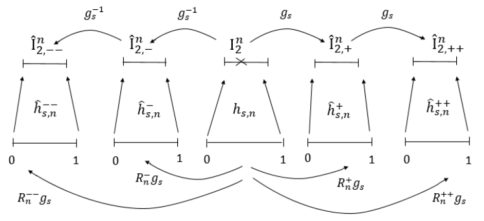
Figure 16:

Lemma 3.1.

Let $s:\mathbb{N}\rightarrow T_{5}$ be proper scaling data such that $g_{s}$ is infinitely renormalizable. Then

$$R_{n}{g_{s}}=g_{\sigma^{n}(s)}.$$

Let $g_{s}$ be infinitely renormalization, then for $n\geq 0,$ we have

$$g_{s}^{5^{n}}:D_{s}\cap I_{2}^{n}\rightarrow I_{2}^{n}$$

is well defined. Define the renormalization $R:U_{\infty}\rightarrow U$ as

$$Rg_{s}=h_{s,1}^{-1}\circ g_{s}^{5}\circ h_{s,1}.$$

The maps $g_{s}^{5^{n}-1}:{\hat{I}}_{2,+}^{n}\rightarrow I_{2}^{n},$   $g_{s}^{5^{n}-2}:{\hat{I}}_{2,++}^{n}\rightarrow I_{2}^{n},$   $g_{s}^{5^{n}-3}:{\hat{I}}_{2,--}^{n}\rightarrow I_{2}^{n},$ and $g_{s}^{5^{n}-4}:{\hat{I}}_{2,-}^{n}\rightarrow I_{2}^{n},$   are the affine homeomorphisms, whenever $g_{s}\in U_{\infty}$. Then

Lemma 3.2.

We have $R^{n}{g_{s}}:D_{\sigma^{n}(s)}\rightarrow[0,1]$ and $R^{n}{g_{s}}=R_{n}{g_{s}}.$

The 3.1 and 3.2 give us the following result,

Proposition 3.3.

There exists a map $g_{{s}^{*}}\in U_{\infty},$ where ${s}^{*}$ is characterized by

$$Rg_{{s}^{*}}=g_{{s}^{*}}.$$

Proof.

Consider $s:\mathbb{N}\rightarrow T_{5}$ be proper scaling data such that $g_{s}$ is infinitely renormalizable. Let $c_{n}$ be the critical point of $g_{\sigma^{n}(s)}.$

The combinatorics for period quintupling renormalization is shown in Figure 17.

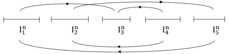
Figure 17: Period quintuple combinatorics ($I_{2}^{n}\rightarrow I_{5}^{n}\rightarrow I_{1}^{n}\rightarrow I_{3}^{n}\rightarrow I_{4}^{n}\rightarrow I_{2}^{n}).$

Figure 18: Length of the intervals and gaps

From Figures 17 and  18, we have the following

$$u_{c_{n}}^{4}(0) =1-s_{5}(n)$$ (3.1)

$$u_{c_{n}}^{5}(0) =u_{c_{n}}(1-s_{5}(n))$$ (3.2)

$$=s_{1}(n)$$

$$u_{c_{n}}^{6}(0) =u_{c_{n}}(s_{1}(n))$$ (3.3)

$$=s_{3}(n)+u_{c_{n}}(0)$$

$$u_{c_{n}}^{7}(0) =u_{c_{n}}(s_{3}(n)+u_{c_{n}}(0))$$ (3.4)

$$=u_{c_{n}}^{2}(0)-s_{4}(n)$$

$$u_{c_{n}}^{8}(0) =u_{c_{n}}(u_{c_{n}}^{2}(0)-s_{4}(n))$$ (3.5)

$$=s_{2}(n)+u_{c_{n}}^{3}(0)$$

$$c_{n+1} =\frac{u_{c_{n}}^{8}(0)-c_{n}}{s_{2}(n)}\equiv\mathcal{R}(c_{n}).$$ (3.6)

We use Mathematica for solving the Eqns. (3.1), (3.2), (3.3), (3.4) and (3.5), and we obtain the expressions for $s_{1}(n),\;s_{2}(n),\;s_{3}(n),\;s_{4}(n)$ and $s_{5}(n).$
Let $s_{i}(n)\equiv S_{i}(c_{n})$ for $i=1,\ldots,5.$ Since these expressions are too lengthy, we just plotted the graph of each $S_{i}(c).$ The graphs of $S_{i}(c_{n})$ are shown in Figures 19.

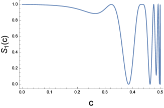
(a)

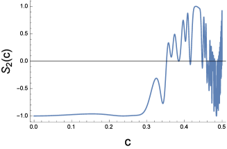
(b)

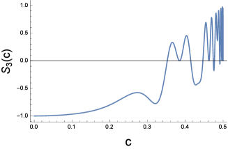
(c)

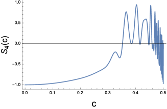
(d)

(e)

Figure 19: The graphs of $S_{1}(c),$ $S_{2}(c),$ $S_{3}(c),$ $S_{4}(c)$ and $S_{5}(c)$

Since $(s_{1}(n),s_{2}(n),s_{3}(n),s_{4}(n),s_{5}(n))\in T_{5},$ then we have the following conditions.

$$s_{i}(n)>0,\textrm{ for each }i\in\{1,2,..,5\}$$ (3.7)

$$\sum_{i=1}^{5}s_{i}(n)<1$$ (3.8)

$$0<c_{n}<\frac{1}{2}.$$ (3.9)

As intervals $I_{i}^{n}$ for $i=1,2,\ldots,5$ are pairwise disjoint, let $g_{l}^{n}$ be the gap between $I_{1}^{n}\;\&\;I_{2}^{n}$ and let $g_{r_{i}}^{n}$ be the gap between $I_{i+1}^{n}$ and $I_{i+2}^{n}$ for $i=1,2,3.$ The intervals and gaps are illustrated in Figure 18. Then we have

$$g_{l}^{n}=u_{c_{n}}^{3}(0)-u_{c_{n}}^{5}(0)\equiv G_{l}(c_{n})>0$$ (3.10)

$$g_{r_{1}}^{n}=u_{c_{n}}(0)-u_{c_{n}}^{8}(0)\equiv G_{r_{1}}(c_{n})>0$$ (3.11)

$$g_{r_{2}}^{n}=u_{c_{n}}^{7}(0)-u_{c_{n}}^{6}(0)\equiv G_{r_{2}}(c_{n})>0$$ (3.12)

$$g_{r_{3}}^{n}=u_{c_{n}}^{4}(0)-u_{c_{n}}^{2}(0)\equiv G_{r_{3}}(c_{n})>0$$ (3.13)

Note that the conditions (3.7), (3.10), (3.11) to (3.13) implies the condition (3.8).

Therefore, the conditions (3.7) and (3.9) together with the gaps conditions (3.10) to (3.13) define the feasible domain $f_{d}$ to be:

$$f_{d}=\Big{\{}c\in(0,0.5):S_{i}(c)>0\;\forall\;i=1,\ldots,5,\;G_{l}(c)>0,\;G_{r_{j}}(c)>0\;\forall\;j=1,2,3\Big{\}}.$$ (3.14)

To compute the feasible domain $f_{d},$ we need to find subinterval(s) of $(0,0.5)$ which satisfies the conditions of (3.14). By using Mathematica, we employ the following command to obtain the feasible domain

$$\textup{N}[\textup{Reduce}[\{S_{1}(c)>0,S_{2}(c)>0,S_{3}(c)>0,S_{4}(c)>0,S_{5}(c)>0,G_{l}(c)>0,G_{r_{1}}(c)>0,$$

$$G_{r_{2}}(c)>0,G_{r_{3}}(c)>0,0<c<0.5\},c]].$$

This yields:

$$f_{d}=(0.379765...,0.384772...)\cup(0.384772...,0.390436...)\equiv f_{d_{1}}\cup f_{d_{2}}.$$

From the Eqn.(3.6), the graphs of $\mathcal{R}(c)$ in the sub-domains $f_{d_{1}}$ and $f_{d_{2}}$ of $f_{d}$ are shown in Figure 20.

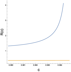
(a) $\mathcal{R}$ has no fixed point in $f_{d_{1}}.$

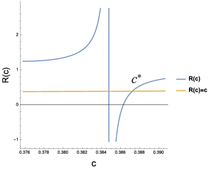
(b) $\mathcal{R}$ has only one fixed point in $f_{d_{2}}.$

Figure 20: The graph of $\mathcal{R}:f_{d}\rightarrow\mathbb{R}$ and the diagonal $\mathcal{R}(c)=c.$

The map $\mathcal{R}:f_{d}\rightarrow\mathbb{R}$ is expanding in the neighborhood of the fixed point $c^{*}$ which is illustrated in Figure 20(b). By Mathematica computations, we observe that $\mathcal{R}$ has a unique fixed point $c^{*}=0.387226...$ in $f_{d_{2}}.$ Therefore, we conclude that $\mathcal{R}$ has only one fixed point in $f_{d}$ such that

$$\mathcal{R}(c^{*})=c^{*}$$

corresponds to an infinitely renormalizable map $g_{s^{*}}.$

In other words, consider the scaling data ${s}^{*}:\mathbb{N}\rightarrow T_{5}$ with

$${s}^{*}(n) =(s_{1}^{*}(n),s_{2}^{*}(n),s_{3}^{*}(n),s_{4}^{*}(n),s_{5}^{*}(n))$$

$$=(u_{c^{*}}^{5}(0),\;u_{c^{*}}^{8}(0)-u_{c^{*}}^{3}(0),\;u_{c^{*}}^{6}(0)-u_{c^{*}}(0),\;u_{c^{*}}^{2}(0)-u_{c^{*}}^{7}(0),\;1-u_{c^{*}}^{4}(0)).$$

Then $\sigma({s}^{*})={s}^{*}$ and using Lemma 3.1 we have

$$Rg_{{s}^{*}}=g_{{s}^{*}}.$$

∎

Lemma 3.4.

If $g_{{s}^{*}}$ is the map with a proper scaling data ${s}^{*}=(s_{1}^{*},s_{2}^{*},s_{3}^{*},s_{4}^{*},s_{5}^{*})$ corresponding to $c^{*},$ then we have

$$(s_{2}^{*})^{2}=s_{5}^{*}.$$

Proof.

Let $\hat{I}_{2,+}^{n}=g_{{s}^{*}}(I_{2}^{n})=[g_{{s}^{*}}(y_{n}),1]$ and $\hat{I}_{5}^{n+1}=g_{{s}^{*}}(I_{5}^{n+1}).$ Then $g_{{s}^{*}}^{5^{n}-1}:\hat{I}_{2,+}^{n}\rightarrow I_{2}^{n}$ is affine, monotone and onto. Further, by construction

$$g_{{s}^{*}}^{5^{n}-1}:\hat{I}_{2,+}^{n+1}\rightarrow I_{5}^{n+1}.$$

Hence,

$$\frac{|\hat{I}_{2,+}^{n+1}|}{|\hat{I}_{2,+}^{n}|}=s_{5}^{*}.$$

Therefore, $|I_{2}^{n}|=(s_{2}^{*})^{n}$ and $|\hat{I}_{2}^{n}|=(s_{5}^{*})^{n}$. Since,

$$g_{{s}^{*}}(y_{n})=u_{{c}^{*}}(y_{n}).$$

This implies,

$$s_{5}^{*}=\frac{|\hat{I}_{2,+}^{n+1}|}{|\hat{I}_{2,+}^{n}|}=\left(\frac{{y_{n+1}}-c}{{y_{n}}-c}\right)^{2}=\left(\frac{|{I}_{2}^{n+1}|}{|{I}_{2}^{n}|}\right)^{2}=(s_{2}^{*})^{2}.$$

∎

Remark 5.

Let $I_{2}^{n}=[y_{n},z_{n}]$ be the interval containing $c^{*}$ corresponding to the scaling data $s^{*}=(s_{1}^{*},s_{2}^{*},s_{3}^{*},s_{4}^{*},s_{5}^{*})$ then

$$g_{s^{*}}(y_{n})=u_{c^{*}}(y_{n}).$$

Hence, $g_{s^{*}}$ has a quadratic tip.

Remark 6.

A proper scaling data $(s_{1}^{*},s_{2}^{*},s_{3}^{*},s_{4}^{*},s_{5}^{*})$ is satisfying the following properties, for all $n\in\mathbb{N},$

1. $\frac{|I_{2}^{n+1}|}{|I_{2}^{n}|}=s_{2}^{*}$ and $\frac{|I_{1}^{n+1}|}{|I_{1}^{n}|}=\frac{|I_{3}^{n+1}|}{|I_{3}^{n}|}=\frac{|I_{4}^{n+1}|}{|I_{4}^{n}|}=\frac{|I_{5}^{n+1}|}{|I_{5}^{n}|}=s_{2}^{*}$

2. $\frac{|I_{1}^{n+1}|}{|I_{2}^{n}|}=s_{1}^{*}$

3. $\frac{|I_{3}^{n+1}|}{|I_{2}^{n}|}=s_{3}^{*}$

4. $\frac{|I_{4}^{n+1}|}{|I_{2}^{n}|}=s_{4}^{*}$

5. $\frac{|I_{5}^{n+1}|}{|I_{2}^{n}|}=s_{5}^{*}$

Remark 7.

The invariant Cantor set of the map $g_{{s}^{*}}$ is next in the complexity to the invariant period tripling Cantor set of piece-wise affine map $f_{{s}^{*}}$ which is described in subsection 2.1. But unlike the Cantor set of $f_{{s}^{*}}$, there are now five ratios at each scale.

In subsection 2.2, we constructed $C^{1+Lip}$ extension of piece-wise affine map $f_{s^{*}}$ to the $C^{1+Lip}$ unimodal map $\mathcal{F}_{s^{*}}.$ A similar construction leads the following result.

Theorem 3.5.

Let $\mathcal{G}_{s^{*}}$ be a $C^{1+Lip}$ extension of $g_{{s}^{*}}.$ Then $\mathcal{G}_{s^{*}}$ is a period quintupling infinitely renormalizable $C^{1+Lip}$ unimodal map with a quadratic tip such that

$$R\mathcal{G}_{s^{*}}=\mathcal{G}_{s^{*}}.$$

As we discussed the topological entropy in subsection 2.3 and the $\epsilon-$variation on scaling data in subsection 2.4, in the similar way, the following results hold for period quintupling renormalization.

Theorem 3.6.

The period quintupling renormalization defined on $C^{1+Lip}$ unimodal maps has infinite entropy and it has a continuum of fixed points.

Theorem 3.7.

There exists an infinitely renormalizable $C^{1+Lip}$ unimodal map ${k}$ with quadratic tip such that $\{c_{n}\}_{n\geq 0}$ is dense in a Cantor set, where $c_{n}$ is the critical point of $R^{n}k$ and $R$ is the period quintupling renormalization operator.

4 Conclusions

In this work, we showed that the period tripling and period quintupling renormalization operators both have a fixed point corresponding to the given proper scaling data. Also, we notice that the geometry of the invariant Cantor set of the map $g_{{s}^{*}}$ is more complex than the geometry of the invariant Cantor set of $f_{{s}^{*}}.$  Furthermore, the piece-wise affine period tripling and quintupling renormalizable maps are extended to a $C^{1+Lip}$ unimodal map. Finally, we showed that the period tripling and period quintupling renormalizations defined on the space of $C^{1+Lip}$ unimodal maps have positive entropy. In fact, the topological entropy of renormalization operator $R$ is unbounded. We proved the existence of an infinitely renormalizable $C^{1+Lip}$ unimodal map $k$ with quadratic tip such that $\{c_{n}\}_{n\geq 0}$ is dense in a Cantor set. This gives us the existence of continuum of fixed points of period tripling and period quintupling renormalizations. This shows non-rigidity of period tripling and quintupling renormalizations.

References

References

- [1] Feigenbaum M J 1978, Quantitative universality for a class of non-linear transformations, J. Stat. Phys., 19 25-52.
- [2] Feigenbaum M J 1979, The universal metric properties of nonlinear transformations, J. Stat. Phys., 21 669-706.
- [3] Coullet P, Tresser C 1978, Itération d’endomorphisms et groupe de renormalisation, J. Phys. Colloque , C5 25-28.
- [4] Lanford-III, O.: 1984, A computer assisted proof of the feigenbaum conjecture , Bull. Amer. Math. Soc. (N.S. ), 6 427-434.
- [5] Lyubich M 1999, Feigenbaum-coullet-tresser universality and Milnor’s hairiness conjecture, Ann. of Math., 149 319-420.
- [6] Davie A M 1999, Period doubling for mappings, Commun. Math. Phys., 176 262-272.
- [7] Faria E de , Melo W de, Pinto A 2006, Global hyperbolicity of renormalization for unimodal mappings, Ann. of Math., 164 731-824.
- [8] Chandramouli V V M S, Martens M, Melo W de, Tresser C P 2009, Chaotic period doubling, Ergodic Theory and Dynamical Systems, 29 381-418.
- [9] Birkhoff G, Martens M, Tresser C 2003, On the scaling structure for period doubling, Astérisque, 286 167-186.
- [10] Tresser C 1991, Fine Structure of Universal Cantor Sets, Instabilities and Nonequilibrium Structures III, E. Tirapegui and W. Zeller Eds., (Kluwer, Dordrecht/Boston/London . 27-42.
- [11] Welington de Melo & Sebastian van Strien, One-Dimensional dynamics, (Springer Verlag, Berlin; 1993).