Comprehensive Probabilistic Tsunami Hazard Assessment in the Makran Subduction Zone

Parastoo Salah^,1, Jun Sasaki,² Mohsen Soltanpour³

¹Graduate Program in Sustainability Science-Global Leadership Initiative, Graduate School of Frontier Sciences, The University of Tokyo, Kashiwa, Chiba, 277-8563, Japan, ²Department of Socio-Cultural Environmental Studies, Graduate School of Frontier Sciences, The University of Tokyo, Kashiwa, Chiba, 277-8563, Japan ³Department of Civil Engineering, K. N. Toosi University of Technology, No. 1346, Vali-Asr St., Tehran, Iran

  Abstract After the 2004 and 2011 tsunamis came unprecedented to the scientific community the role of probabilistic tsunami hazard assessment (PTHA) in tsunami-prone areas came to the fore. The Makran subduction zone (MSZ) is a hazardous tsunami-prone region; however, due to its low population density, it is not as prominent in literature. In this study, we assess the threat of tsunami hazard posed to the coast of Iran and Pakistan by the MSZ and present a comprehensive PTHA for the entire coast regardless of population density. We accounted for sources of epistemic uncertainties by employing event tree and ensemble modeling. Aleatory variability was also considered through probability density function. Further, we considered the contribution of small to large magnitudes and used our event trees to create a multitude of scenarios as initial conditions. Funwave-TVD was employed to propagate these scenarios. Our results demonstrate that the spread of hazard curves for different locations on the coast is remarkably large, and the probability that a maximum wave will exceed 3 m somewhere along the coast reaches $\{13.5,25,52,74,91\}$ for return periods $\{50,100,250,500,1000\}$, respectively. Moreover, we found that the exceedance probability could be higher at the west part of Makran for a long return period, if we consider it as active as the east part of the MSZ. Finally, we demonstrated that the contribution of aleatory variability is significant, and overlooking it leads to a significant hazard underestimation, particularly for a long return period.

 

1 Introduction

Tsunami events are infrequent in several water bodies around the world, yet their danger cannot be ignored due to the high levels of destruction that follow, including major losses of life and property damage. In particular, the importance of a comprehensive tsunami hazard assessment (THA) is highlighted when a disastrous tsunami occurs. Recent devastating tsunamis such as the Sumatra tsunami of 2004, with more than 200,000 fatalities (Starrs, 2014), and the 2011 Tohoku tsunami in Japan, which caused more than 15,000 fatalities and was responsible for the Fukushima Nuclear Power Plant accident (Fujii et al., 2011), are representative examples. Following these disasters, there has been a remarkable development in tsunami risk management to reduce the effect of future tsunamis. For recent reviews of these developments, including full lists of references, see (Løvholt et al., 2015; Ward et al., 2020).

Tsunami hazard assessment includes sensitivity analyses (see e.g. (Goda et al., 2014, 2019)) as well as deterministic (see e.g. (Lynett et al., 2016; Heidarzadeh et al., 2009; Salah and Soltanpour, 2014)) and probabilistic approaches. The latter approach– called the probabilistic tsunami hazard assessment (PTHA) –has received substantially increased attention after the 2004 and 2011 tsunamis (Satake, 2014; Kagan and Jackson, 2013; Lorito et al., 2015; Løvholt et al., 2014). Unlike deterministic approaches that consider specific scenarios (commonly including the worst case scenario) to calculate tsunami hazard metrics (such as run up height and arrival time), PTHA calculates the likelihood of tsunami impact employing multiple possible scenarios consisting of the contributions from small to large events along with all quantifiable uncertainties (Geist and Lynett, 2014). Hence, PTHA can overcome the limitation of incomplete or insufficient historical records, and extend the return periods from hundreds to thousands of years. Furthermore, this approach considers the uncertainties stemming from the lack of researcher knowledge and the random nature of hazards. The former is represented by epistemic uncertainty in literature while the latter is known as aleatory variability. These concepts are explained in detail in section 2.1.

PTHA was developed by adopting the probabilistic seismic hazard analysis (PSHA) (Cornell, 1968; Rikitake and Aida, 1988; Downes and Stirling, 2001), and much progress has been built upon it see (Grezio et al., 2017) and the references therein. Notwithstanding that PTHA is a relatively new method, it has been widely used in tsunami-prone areas owing to its diverse range of applications (e.g., (Thio et al., 2014; Davies and Griffin, 2019; Mori et al., 2018)), each of them covers different uncertainties, methods, and level of accuracy. In this study, we assessed the tsunami hazard using the probabilistic approach in the Makran subduction zone (MSZ).

The MSZ is a tsunami risk zones as attested by compiled tsunami catalogues and recent paleotsunami studies (Kakar et al., 2015) that exhibits risks for the neighboring countries of Iran, Oman, and Pakistan. This region is not as prominent in scientific literature as other tsunami-prone subduction zones owing to its low population density, and it remains as one of the least studied regions. The authors of (Heidarzadeh and Kijko, 2011) performed the first generation of PTHA in the MSZ. Their results are not reliable for return period far from the typical recurrence time of magnitude $M_{\text{w}}=8.1$ because only three earthquakes were considered in their study. Furthermore, the rough discretization of sources used may have affected the final results.  (Hoechner et al., 2016) conducted a PTHA along the MSZ based on a synthetic earthquake catalogue. In their study, a simple geometry model along with a uniform (cf. heterogeneous) slip distribution were used because their primary focus was identifying the consequences of maximum magnitude assumptions. Finally, (El-Hussain et al., 2016) performed a logic tree approach for assessing the hazard only for Oman coasts. Of particular importance is the absence of aleatory variability in the aforementioned studies. For any tsunami probability study, it is critical to understand how uncertainty affects probability estimation. Thus, we aim to fill the gaps of previous PTHA studies in the MSZ via developing a methodology that incorporates both aleatory and epistemic uncertainties. Our work overcomes the limitation in the integration of uncertainties, namely, tidal level, heterogeneity in slip distribution and rupture size, numerical and geometry models, earthquake recurrence rate, and maximum magnitude.

First, we quantified the epistemic uncertainties of fault source for the assessment of mean annual rates of earthquakes at different magnitude levels. Despite the more classical approaches commonly used in literature, we employed event tree and ensemble modeling, which is based on a method initially introduced for PSHA studies (Marzocchi et al., 2015). To develop our event tree, we utilized available seismic, geodetic, and historical catalogue data to better understand the potential seismogenic zone, maximum magnitude, and recurrence model for the MSZ. Next, rupture complexity, namely, dimensions, slip distribution, and possible earthquake locations, were considered to develop scenarios. Then, a high-resolution tsunami numerical model was used to propagate tsunami waves resulting from these scenarios. Finally, we consider the aleatory variability associated with tidal variations, tsunami numerical and bathymetric models, and scaling relations through statistical methods. We followed these specific intermediate steps to derive the probability of tsunami height occurrence and exceedance for a given exposure time along the Iran and Pakistan coasts. We also compared our results obtained in the presence and absence of the aleatory variability. Our findings provide information for various stakeholders to underpin tsunami risk activities, such as insurance activity, land use and city planning, critical facility design, and mitigation measure design and implementation.

2 Methodology and Dataset

Our methodology aims to calculate the probability of exceeding a set of tsunami heights at the Makran coast, considering both epistemic and aleatory uncertainties. In this work, we only focused on tsunamis induced by earthquakes; landslide-induced tsunamis were beyond the scope of our research and should be addressed in future work. Fig. 1 demonstrates a summary of our framework. First, we determined the seismicity area and generated synthetic scenarios similar to that described by (Davies and Griffin, 2019). Then, for each scenario, we ran a fully nonlinear tsunami model Funwave-TVD (Kirby et al., 1998; Shi et al., 2012) to obtain the maximum wave heights along the coastline. Additionally, we incorporated the epistemic uncertainties by developing two event trees and ensemble modeling. Finally, we calculated the tsunami height exceedance rate considering the aleatory variability.

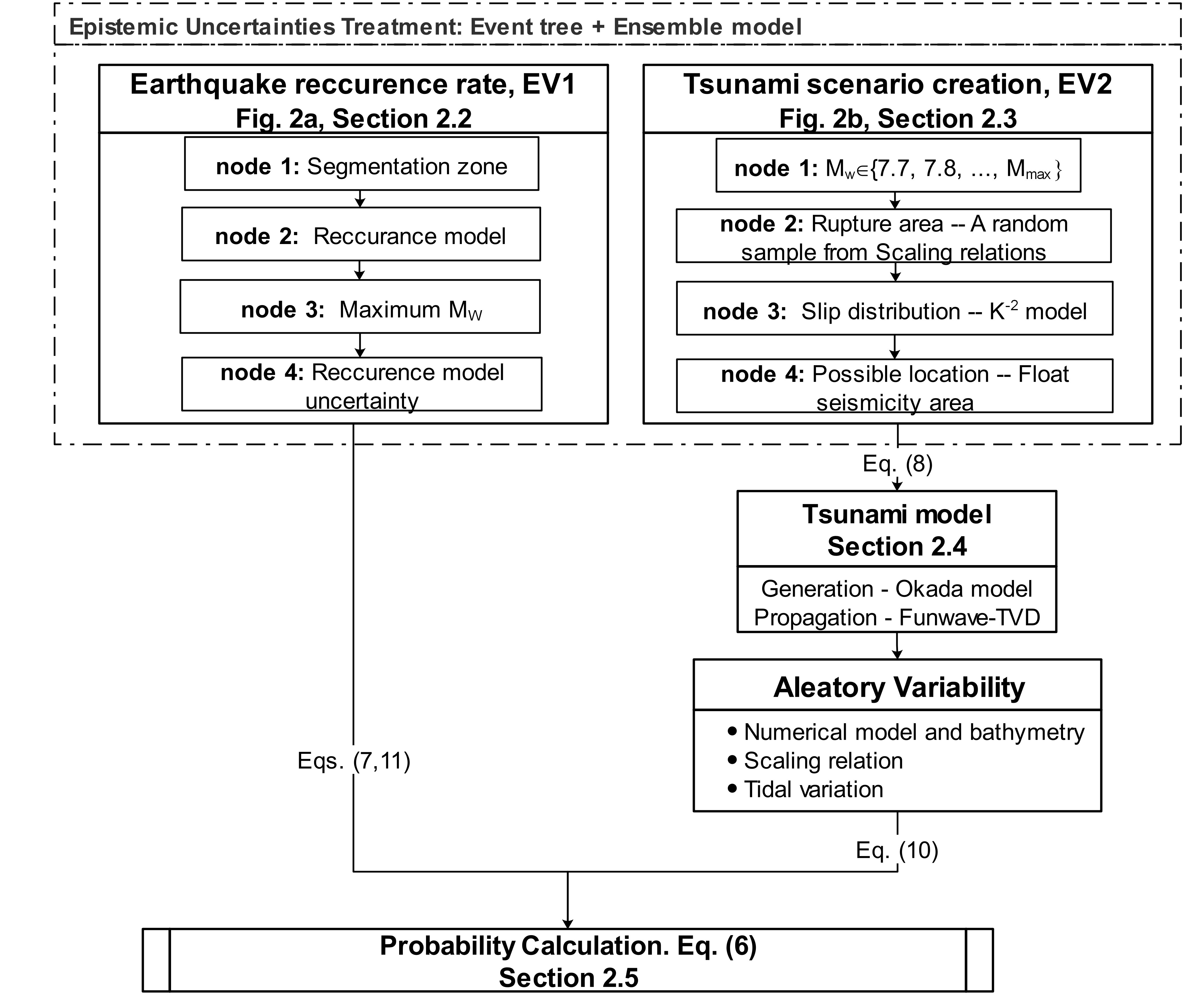
Figure 1: Methodology framework. First, the fault geometry was defined using SLAB 2.0, and the source was discretized into smaller segments. Next, two event trees were developed to define the earthquake recurrence rate and create tsunami scenarios; then, the Okada model and Funwave-TVD were used to calculate tsunami heights for our scenarios. Finally, considering the aleatory variability, we derived the probability of exceedance.

2.1 Treatment of uncertainties

A reliable PTHA must consider the epistemic uncertainty and aleatory variability simultaneously. The latter expresses the innate variability of the physical process, while the former is related to the lack of understanding and limited knowledge of the process. As shown in Fig. 1, each factor was considered as described in detail below.

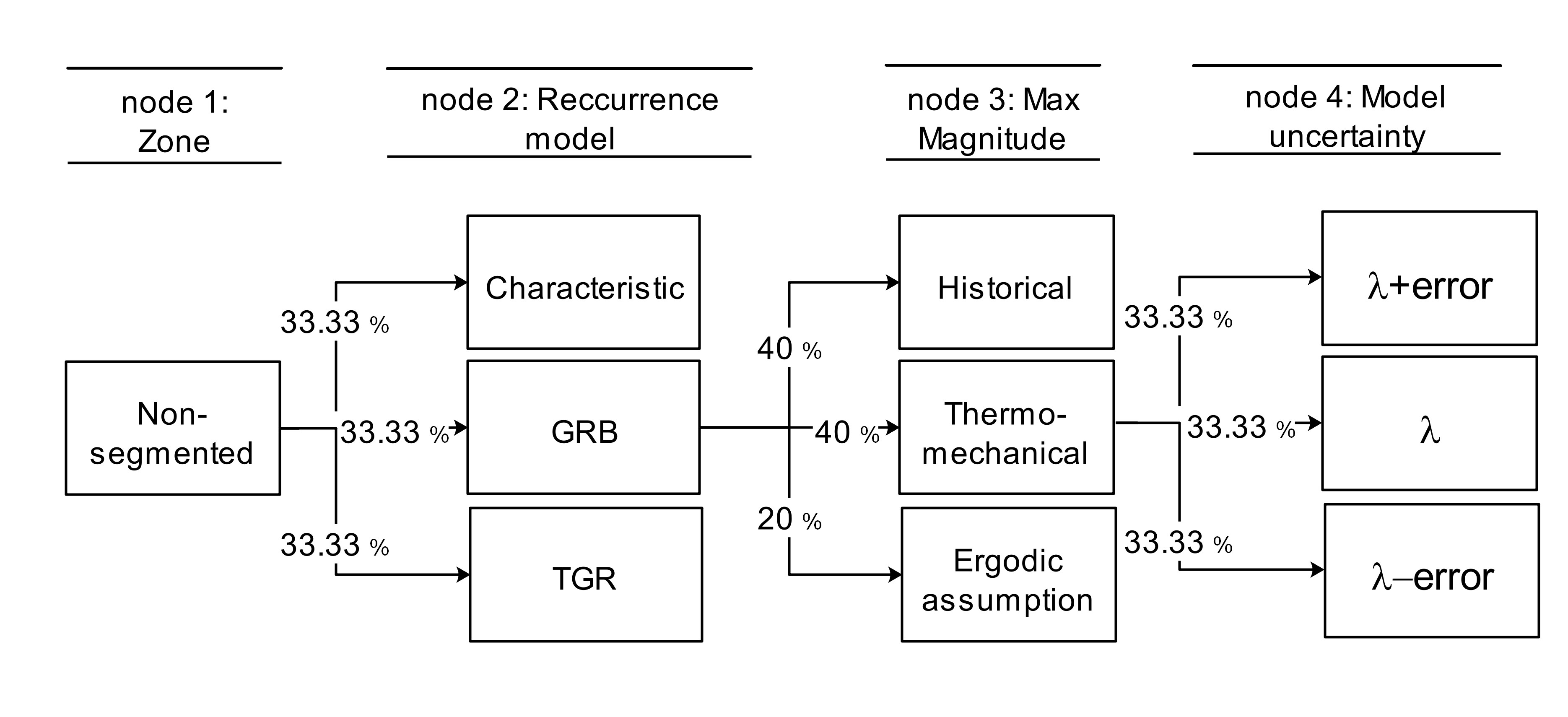
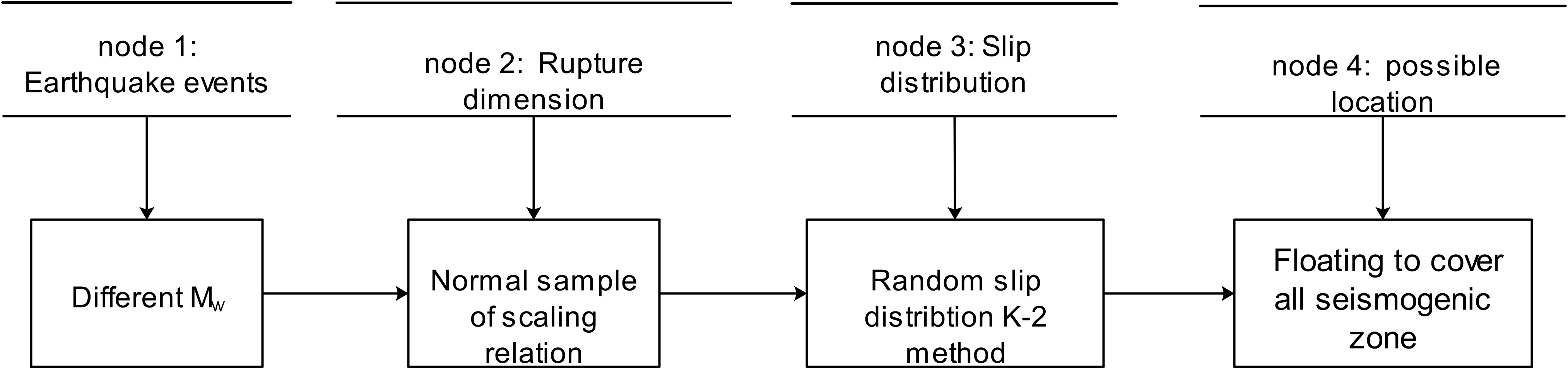
(a)

(b)

Figure 2: Developed event trees for (a) source recurrence model; (b) rupture complexity and tsunami scenario creation.

2.1.1 Epistemic

Epistemic uncertainties can be incorporated by developing event trees (Annaka et al., 2007). We developed two event trees:

1. Focusing on the fault source recurrence model for the assessment of mean annual rates of earthquakes at different magnitude levels with 27 branches. It consists of three approaches for the seismicity model [Gutenberg–Richter–Bayes (GRB) (Kijko et al., 2016), truncated Gutenberg–Richter, and characteristic (Kagan, 2002)]; three maximum magnitudes ($M_{\text{max}}$) [based on the Kijko–Sellevoll–Bayes method (Kijko, 2004), thermomechanical modeling (Smith et al., 2013) and ergodic assumption (Bird and Kagan, 2004)]; and three for incorporating the uncertainty of the earthquake occurrence model. See Fig. 2

2. Focusing on the bulk rupture parameters and rupture complexity. It consists of rupture length and width, earthquake source location within the fault, and slip distribution. See Fig. 2

2.1.2 Aleatory

The proper treatment of aleatory variability in tsunami wave heights is a prominent subject, and ignoring this typically leads to significant hazard underestimation (Bommer and Abrahamson, 2006). In our analysis, we have identified three main contributions, i.e., $\{\sigma_{\text{m}},\sigma_{\text{s}},\sigma_{\text{t}}\}$, to the aleatory variability as below.

Numerical model and bathymetry ($\sigma_{\text{m}}$) –

Due to the lack of field data and background information on the MSZ, the 2011 Tohoku earthquake of Japan was modeled, and the results were compared with the available measured data to quantify the mismatch between the observed and computed tsunami heights. This uncertainty is described as the standard deviation of a log-normal distribution with a zero mean (Aida, 1978; Thio et al., 2007):

$$\sigma_{\text{m}} =\log\kappa=\sqrt{\frac{1}{n}\sum_{i=1}^{n}(\log K_{i})^{2}-(\log K)^{2}}\,,$$ (1)

$$\log K =\frac{1}{n}\sum_{i=1}^{n}\log\left(\frac{H_{\text{obs, }\!i}}{H_{\text{model, }\!i}}\right)\,.$$

Here, $K_{i}=H_{\text{obs, }\!i}/{H_{\text{model, }\!i}}$ with $H_{\text{obs, }\!i}$ and $H_{\text{model, }\!i}$ being the measured and simulated tsunami heights at the $i^{\text{th}}$ station, respectively. For $H_{\text{obs}}$, the measured tsunami height at GPS, DART buoys, and tide and wave gauges were used. Moreover, we simulated the 2011 Tohoku tsunami using the same bathymetry and numerical model as the ones we used for the MSZ to obtain $H_{\text{model}}$ (see section 2.4). Fig. 3 shows the comparison between the modeled and measured tsunami heights with $\sigma_{\text{m}}=0.376$.

Scaling relations ($\sigma_{\text{s}}$) –

Given the earthquake magnitude, rupture length and width were derived by evaluating the scaling relations. To do so, we used Strasser relations (Strasser et al., 2010) as explained in section 2.3.2. To account for stochasticity in the earthquake dimensions imposed by the scaling relations, we used the standard deviations associated with the equations, which were $\sigma_{\text{s}_{1}}=0.173$ and $\sigma_{\text{s}_{2}}=0.180$ for length and width, respectively. The variability in scaling relations was derived from a regression analysis of the relations (Strasser et al., 2010, Table 1). $\sigma_{\text{s}}=\sqrt{\sigma_{\text{s}_{1}}^{2}+\sigma_{\text{s}_{2}}^{2}}$= 0.249 was used in combination with the other sources of aleatory variability (see section 2.5).

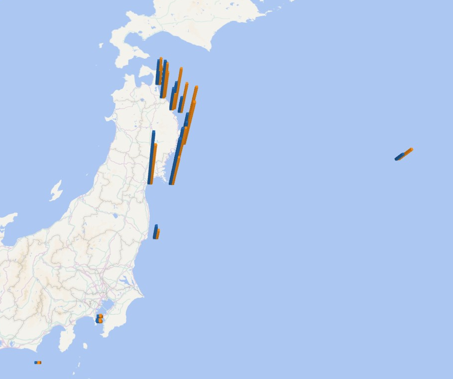
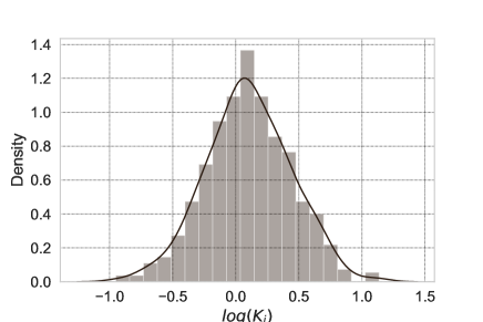
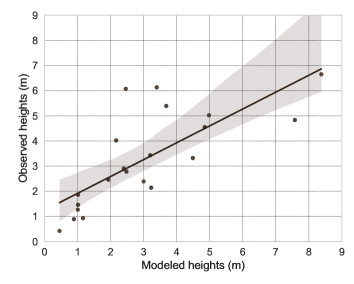
Figure 3: Comparison between modeled and measured tsunami height for the 2011 Japan tsunami at 15 stations recorded by GPS, DART buoys, tide and wave gauges; regression line for modeled versus measured height (bottom right); histogram of errors in log tsunami height and corresponding normal distribution (bottom left).

Tide ($\sigma_{\text{t}}$) –

Because the tide level at tsunami arrival time is unknown, tidal variation variability must be included in the PTHA. In the Makran region, the tidal variation is notable, and the peak-to-peak tidal amplitude is as high as $2$-$3$ m. For this task, we calculated the probability of exceedance of mean sea level (MSL) from the tidal record at each point of interest (PoI).

To calculate tidal record probability, we used a relatively long time-series of record measured by tidal gauges for each PoI. For PoIs in which a tidal record is not available, we used a linear interpolation of the closest tidal gauges. This choice seems reasonable because the differences in tidal levels along the Makran coast are not significant (Akbari et al., 2017). Fig. 4 illustrates an example of our methodology for one PoI, Beris. $\sigma_{\text{t}}$ for the remaining PoIs are presented in Online Resource 1.

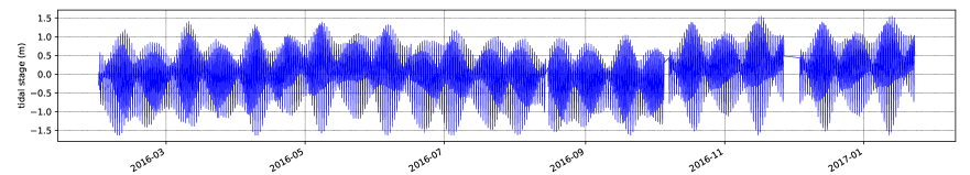
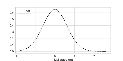
Figure 4: Tidal time series record of one year starting from 2016 for Beris (top); corresponding normal distribution (bottom). For this PoI, $\sigma_{\text{t}}=0.612$.

2.2 Source

The MSZ is located on the southeastern coasts of Iran and southern coasts of Pakistan. This zone extends east from the Strait of Hormoz to the Ornch–Nal Fault in Pakistan. It experienced the deadliest tsunami that has occurred in the Indian Ocean prior to 2004, and recent smaller earthquakes suggest seismicity on the megathrust. However, poor historical records have led to significant uncertainty and complicated hazard potential estimation. Therefore, as mentioned in section 2.1.1, to incorporate the uncertainties associated with the fault source, we developed an event tree (EV1) to assess the mean annual rates ($\nu_{j}$) of earthquakes at different magnitude levels, as described below.

2.2.1 Zone: node 1 in EV1

The eastern and western parts of the MSZ exhibit extremely different seismicity patterns (Aldama-Bustos et al., 2009). This, along with its unrecognized bathymetric trench, makes the MSZ a unique subject of analysis.  (Al-Lazki et al., 2014) argued that the eastern MSZ is underlain by an oceanic lithosphere, while the western part is possibly underlain by a continental or very low velocity oceanic lithosphere. This, along with the more historical seismicity activity at the eastern part, form the hypothesis of east-west segmentation of the MSZ. However, it remains a controversial issue whether the MSZ should be considered segmented in hazard studies because the existence of late Holocene marine terraces along the eastern and western halves suggests that both can generate megathrust earthquakes (Normand et al., 2019).

Owing to the above mentioned related controversy, we neglected the hypothesis of the segmented MSZ as it leads to a strong hazard underestimation.  Accordingly, this study considers only the non-segmented rupture.

2.2.2 Recurrence rate model: node 2 in EV1

The severity of a large earthquake is determined by the tail of a frequency distribution. Thus, earthquake catalogues are limited at large magnitudes for a particular fault zone. This makes the accurate estimation of the probabilistic tsunami hazard through the application of the recurrence interval of seismic history impossible. In particular, for MSZ with poor and incomplete catalogues, a simple linear regression of the historical cumulative distribution is known to be biased (Power et al., 2012). Accordingly, several models exist that can be used to define the distribution of earthquake magnitudes for incomplete catalogues. In this study, we used three seismicity models:

1. Gutenberg–Richter–Bayes(GRB) (Kijko et al., 2016). Seismicity was determined using the HA3 application built in MATLAB. The applied procedure of the seismic hazard considers the incompleteness of the seismic catalogues, uncertainty in magnitude estimation, and variation in seismicity. The code accepted mixed data catalogues, namely, paleo, historical, and instrumental with different completeness magnitudes, time periods, and magnitude uncertainties. This method employed a mixed (Bayesian) Poisson-gamma distribution as a model of earthquake occurrence over time.

2. Characteristic (Kagan, 2002). The characteristic distribution has the cumulative complementary function ($\Phi_{M}$) truncated on both ends and is characterized by the following equation

   $$\Phi_{M}=\Bigg{\{}\begin{array}[]{lr}e^{-\beta(M-M_{\text{min}})}\hskip 14.22636pt\text{for }&M_{\text{min}}\leq M\leq M_{\text{max}}\\ {}&{}\hfil\\ 0\hskip 65.44142pt\text{for }&M>M_{\text{max}}\end{array}\,.$$ (2)

3. Truncated Gutenberg-Richter (TGR). The cumulative complementary function ($\Phi_{M}$), which is truncated at both ends, is expressed as

   $$\Phi_{M}=\Bigg{\{}\begin{array}[]{lr}\frac{e^{-\beta(M-M_{\text{min}})}-e^{-\beta(M_{\text{max}}-M_{\text{min}})}}{1-e^{-\beta(M_{\text{max}}-M_{\text{min}})}}\hskip 14.22636pt\text{for }&M_{\text{min}}\leq M\leq M_{\text{max}}\\ {}&{}\hfil\\ 0\hskip 129.17531pt\text{for }&M>M_{\text{max}}\end{array}\,,$$ (3)

   where $M_{\text{min}}$ is the level of magnitude completeness, $M_{\text{max}}$ is the maximum possible earthquake magnitude and $\beta=b\log 10$, and $b$ is the parameter of the Gutenberg-Richter relation.

2.2.3 $M_{\text{max}}$: node 3 in EV1

PTHAs are more sensitive to $M_{\text{max}}$ than PSHAs because tsunami heights do not saturate with increasing magnitude as seismic ground motions do (Thio et al., 2007). $M_{\text{max}}$ based on instrumental catalogues may underestimate the maximum magnitude event due to their short records. Here, to include this uncertainty, we used three methods for maximum magnitude ($M_{\text{max}}$) assessment:

1. Kijko-Sellevoll-Bayes method (Kijko, 2004): using the HA3 application, we found $M_{\text{max}}=8.2$.

2. Thermomechanical model: we observed a potential of $M_{\text{max}}=9.22$ for the full length of subduction zone in (Smith et al., 2013).

3. Ergodic assumption: (Bird and Kagan, 2004) suggested $M_{\text{max}}=9.58$ for subductions based on their statistical analysis for a number of faults worldwide. However, this is an implausible event in comparison to the aforementioned maximum magnitudes (Frohling and Szeliga, 2016). Thus, a smaller weight (20 $\%$), was assigned to this branch of our event tree.

2.2.4 Earthquake catalogues

Earthquake data employed in this study were derived from various sources: (i) International Seismological Centre (ISC) (ii) Incorporated Research Institutions for Seismology (IRIS) (iii) The United States Geological Survey Online bulletin (USGS), which includes information from the National Ocean and Atmospheric Administration (NOAA) and Preliminary Determination of Epicentres (PDE) provided by the National Earthquake Information Center (NEIC) (iv) Global Historical Earthquake Archive (GEM) (v) Iranian Seismological Center (IRSC) . Extra effort has been made to extract additional data from literature regarding earthquakes with magnitudes beyond 6.5. This includes information from the Pakistan Meteorological Department (PMD) (Department], 2007) and (Ambraseys and Melville, 1982).

We compiled the catalogues for a region that lies in the plate interface, excluding nonsubduction seismicity (see Fig. 5). The catalogues cover the period from 825 BCE to mid-2020 CE. These catalogues are different in terms of magnitude scale. When available, the moment magnitude, $M_{w}$, was used; otherwise, the published magnitudes (e.g., teleseismic magnitudes and modified Mercalli intensity) were converted to $M_{w}$ using the empirical $laws$ proposed by (Allen et al., 2012; Lolli et al., 2014).

We used the ZMAP7 analysis tool (Reyes and Wiemer, 2019) to prepare the catalogues for our recurrence models. First, following the assumption that seismicity obeys a Poisson process, it is necessary to decluster the catalogues by removing all dependent events, namely, precursors and aftershocks. Hence, we employed the cluster approach proposed by Reasenberg (Reasenberg, 1985) to eliminate dependent shocks. Then, duplicate events from different catalogues were removed. Sunsequently, the plot of the cumulative number of events allowed us to split the working catalogues into prehistorical, historical, and three sub-instrumental categories. Each has a different magnitude of completeness ($M_{c}$) and magnitude uncertainty. Moreover, we obtained a prior value for $b$ in each catalogue to use in our recurrence models (see Table 1).

Table 1: Extracted values for magnitude of completeness ($M_{c}$), error, and $b$-value from zmap for different working catalogues.

	prehistorical	historical	complete 1	complete 2	complete 3
period	$326\text{ BC }-1020$ AD	$1480-1899$	$1900-1963$	$1964-1989$	$1990-2020$
$M_{c}$	—	$5.5$	$5.7$	$4.8$	$4.8$
error value	$0.6$	$0.5$	$0.45$	$0.35$	$0.25$
prior $b$-value	$0.91\pm 0.04$

2.3 Tsunami scenarios

To create possible tsunami scenarios and incorporate rupture and location uncertainties, event tree 2 (EV2) was developed (see Fig. 2). The branches of EV2 are introduced in section 2.1.1; here, we describe them in detail.

2.3.1 Source discretization

Similar to (Davies and Griffin, 2019), fault geometry was defined using a three-dimensional source zone fault-plane, SLAB 2.0 – a comprehensive subduction zone geometry model (Hayes et al., 2018). The MSZ has an extremely shallow subduction angle (dip) and thick sediment pile ($\approx 7$ km) that leads to a wide potential seismogenic zone (Smith et al., 2013). Following the suggestion of (Berryman et al., 2015) and (Safari et al., 2017), we constrained the seismogenic zone from 0 km (i.e., trench) to $38$ km depth as a preferred down-dip limit. This assumption leads us to define a seismogenic zone for the MSZ as shown in Fig. 5.

Then, to obtain a better representative of the MSZ fault geometry, we discretized our seismogenic zone into $50\times 50$ km² segments. Finally, dip, rake, strike, and depth for each segment were identified for use in the Okada model (Okada, 1985) to generate the initial tsunami conditions. The fault parameters for all the segments are presented in Online Resource 2.

2.3.2 Rupture area: node 1 and 2 in EV2

For each magnitude ranging from $M_{w}=7.7$ to $M_{w}=9.5$ with a regular magnitude interval of 0.1, i.e., $M_{w}\in\{M_{w,\text{min}},M_{w,\text{min}}+0.1,\ldots,M_{w,\text{max}}-0.1,M_{w,\text{max}}\}$, we calculated the rupture length and width using the scaling relation of Strasser derived from the regression analysis of historical subduction events (Strasser et al., 2010, Table 1). For $M_{w}\leq 8.7$, we included uncertainties associated with the use of the scaling relation for earthquake dimensions as described in section 2.1. However, we observed that the variability enlarges with growing magnitude. Hence, for $M_{w}>8.7$, rather than using only one value for rupture length and width, a random sample was selected from a log-normal distribution. Our initial intention was to consider the dependence of the variance of rupture length and width, and sample from a two-dimensional multivariate normal distribution (Blaser et al., 2010). However, we noticed that the range of variation was quite small. Considering our segmentation size (i.e., $50\times 50$ km²), the independent random selection of length ($L$) and width ($W$) were generated form normal distributions according to

$$\log_{10}L\sim\mathcal{N}(-2.477+0.585M_{w},0.18)\,,$$ (4)

$$\log_{10}W\sim\mathcal{N}(-0.882+0.351M_{w},0.173)\,.$$

Here, $\mathcal{N}(\mu,\sigma)$ is a normally distributed random variable with mean $\mu$ and standard deviation $\sigma$; notation $\sim$ denotes the equivalence of distributions.

Then, for each length and width we calculated the number of segments downdip ($n_{s}$) and along-strike ($n_{l}$) using the method described in (Davies et al., 2018, Eq. (4)).

2.3.3 Slip distribution: node 3 in EV2

Slip distribution significantly affects tsunami heights nearshore. Recently, different studies have shown that maximum nearshore wave height varies by a factor of 2 or more due to heterogeneity in earthquake slip (Løvholt et al., 2012; Mueller et al., 2015; Goda et al., 2014; Sugino et al., 2015; Butler et al., 2017). However, owing to its convoluted nature and computation complexity, tsunami hazard assessments are usually based on idealized uniform slip earthquakes. In this work, we used a uniform slip for $M_{w}\leq 8.7$, where the effect of spatial slip distribution is not significant, and heterogeneous slip distribution for $M_{w}\geq 8.8$, where we found that the heterogeneity of slip notably varies tsunami heights at our PoIs. This trade-off was specified to account for the effect on tsunami heights and optimize the number of scenarios through our sensitivity analysis. The number of scenarios and differences among modeled tsunami heights at PoIs were compared for a fixed scenario, but with varying $M_{w}$, starting from $M_{w}=7.7$.

This observation is similar to (Sugino et al., 2015) in which, for the Japan PTHA, earthquakes with $M_{w}>8.9$ were considered large, and the authors included three levels of spatial slip in their model.

Average slip was computed for each scenario with magnitude $M_{w}$ employing the scaling relation as follows:

$$M_{w}=\frac{\log M_{o}-9.1}{1.5}\,,\qquad\qquad S=\frac{M_{o}}{\mu\times A}\,,$$ (5)

where $M_{o}$ is the seismic moment, $\mu$ the shear modulus, and $A$ the area of each scenario. We set $\mu=3\times 10^{11}$ dyn cm^-2 as it is appropriate for crustal rocks and shallow depth faults (Deif and El-Hussain, 2012). We then used the evaluated $S$ from Eq. (5) as a uniform slip for $M_{w}\leq 8.7$; whereas for $M_{w}>8.7$, the slip for each sampled ($L$,$W$)-scenario was created randomly using the PTHA18 code built in R. The PTHA18 code uses the SNCF model of (Davies et al., 2015) for generating random slip distribution for a given segment dimension and number. This model is a variant on the widely used $K^{2}$ model. Further implementation details can be found in (Davies, 2019) and (Davies et al., 2015).

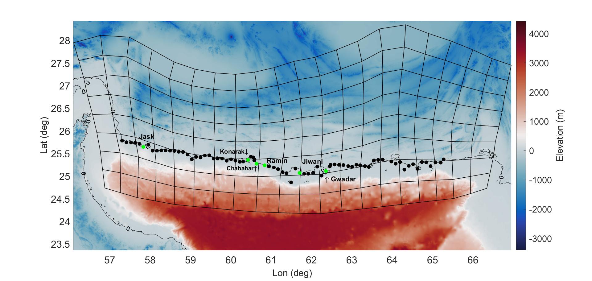
Figure 5: Elevation (m) and computational domain; dots represent PoIs located at 0 m isobath along the coast; black mesh indicates the seismogenic zone and source discretization into $50\times 50$ km².

2.3.4 Possible location: node 4 in EV2

To cover all the seismogenic zone for each magnitude and sampled length and width, we floated the calculated $n_{s}\times n_{l}$ through all possible locations of the Makran seismicity area, shown in the blue mesh in Fig. 5. We assumed that the occurrence of a specific magnitude was equally probable in all possible locations; therefore, an equal weight was assigned to the branches of EV2.

2.3.5 Analysis of the number of scenarios

In this section, we describe the number of scenarios based on the method explained in the previous subsections. Moreover, a justification to confirm the sufficiency of the number of scenarios is provided. A uniform slip distribution was used when the difference in the mean value of all the PoIs along the coast was $\leq 0.5$ m. The number of scenarios increases in lower magnitudes (due to the rupture size, thereby floating it to cover all the seismicity areas); however, the tsunami heights at PoIs were not significant, employing heterogeneous distribution. Hence, for $M_{w}\leq 8.7$ (which was the threshold to indicate the difference in tsunami heights due to the heterogeneity in slip distribution) we used a uniform slip distribution. For $M_{w}\geq 8.7$, a specific number of heterogeneous slip distributions (from 10 to 18) was used. We used the technique introduced in (Mulia et al., 2020) to demonstrate that the number of considered slip distributions for each magnitude is sufficient. Hence, we calculated the coefficient of variation $CV=\sigma_{\text{h}}/\mu_{\text{h}}$, where $\sigma_{\text{h}}$ and $\mu_{\text{h}}$ are the standard deviation and mean of maximum tsunami heights at all the PoIs, respectively. The results are illustrated in Fig. 6, where the variation of CV approximately converges to zero for the given number of scenarios for each magnitude level. Table 2 shows the number of scenarios for different magnitude levels based on the method described above.

Table 2: Number of scenarios for each magnitude considering the heterogeneity of the slip.

$M_{w}$	$n_{s}$	$n_{l}$	Possible scenarios along-strike	Possible scenarios down-dip	Total Possible scenarios	Total Possible Scenarios
7.7	2	1	19	7	133	133
7.8	2	2	19	7	133	133
7.9	3	2	18	7	126	126
8.0	3	2	18	7	126	126
8.1	4	2	17	7	119	119
8.2	4	2	17	7	119	119
8.3	4	2	17	7	119	119
8.4	6	2	15	7	105	105
8.5	6	3	15	6	96	96
8.6	7	3	14	6	84	84
8.7	8	3	13	6	78	78
8.8	9	3	12	6	72	72*10
8.9	11	3	10	6	60	60*12
9.0	13	4	8	5	40	40*13
9.1	15	4	6	5	30	30*15
9.2	16	4	5	5	25	25*18
9.3	19	5	2	4	8	8*18
Sum					1428	4227

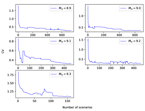
Figure 6: Coefficient of variation of maximum coastal tsunami heights at different level of magnitudes against the number of scenarios.

Alternatively, to justify the number of scenarios, the results of the samples from similar earthquake locations and magnitudes of past earthquake tsunami events can be compared. However, notably, there is a significant disagreement between the results of numerical models and existing measurements, evidence, and witnesses for the 1945 tsunami, which is the only significant tsunami in the MSZ (Okal et al., 2015; Rastgoftar and Soltanpour, 2016; Heidarzadeh and Satake, 2017). This connotes the existence of another mechanism involved in the tsunami generation, such as landslides. Hence, comparing our simulation results with the available data will be neither precise nor beneficial, as we have only considered earthquake-generated tsunamis.

2.4 Tsunami model

In total, 4220 scenarios were created using the approach discussed in the previous section considering the branches of EV2 for different magnitudes, which were randomly sampled from the rupture area, slip distribution, and all possible locations. For each scenario, numerical simulations of tsunami generation and propagation were performed. First, we calculated vertical co-seismic dislocation via a homogeneous elastic half-space model (Okada, 1985). Then, the Kajiura filter (Kajiura, 1963) was used for the ocean surface deformation of the dislocation to calculate the initial conditions. Regarding the simulation of tsunami propagation a fully nonlinear and dispersive Boussinesq long wave model, FUNWAVE-TVD (Kirby et al., 1998; Shi et al., 2012), was employed. It features accurate dissipation by considering the breaking wave and bottom friction processes, and has been systematically validated against experimental studies and benchmarks (Tehranirad et al., 2011). The code was parallelized using the message passing interface (MPI). This scalable algorithm (using more than $90\%$ of the number of cores in a computer cluster (Shi et al., 2012)) has been paved our way for modeling multitude scenarios. The dispersive effects may not always be significant in long tsunami wave trains and considering them is computationally demanding (cf. nonlinear shallow water models) (Tajalli Bakhsh, 2014). However, owing to the MPI protocol, using FUNWAVE-TVD did not cost us notable additional time, given our computational tools. Instead, adopting FUNWAVE-TVD in this study would be useful for future development of multi-scale PTHA from ocean to local inundation covering most of the important processes with higher accuracy, including landslide induced and far-field tsunamis, where wave dispersivity becomes important.

Here, FUNWAVE-TVD was used in its Cartesian implementation. To prevent non-physical reflection from the boundaries, sponge layers were specified with $10$ km thickness within our computational domain. A $600$ m resolution was used for the computational domain, which is a trade-off between precision and practical feasibility (see Online Resource 3). Moreover, the finer grid resolution would be beneficial only if a high-quality bathymetry is available. However, the high-quality bathymetry data does not exist in almost all the selected PoIs.

Here, GEBCO-2020 (global bathymetric model based on ship-track data) model with 15 arc second resolution, combined with limited measured data in shallow water depths by the Ports and Maritime Organization of Iran (PMO), has been used for our tsunami simulations. Each scenario has been simulated for $8$ h, and for each computational time step, a time series of tsunami wave has been recorded at $84$ hazard points. These PoIs are located at $5$ to $0$ m isobath at approximately $10-12$ km intervals along the Iran and Pakistan coastline. The PoIs are shown in Fig. 5.

2.5 Deriving the probability of exceedance

For a given exposure time ($\Delta T$), PTHA was performed by deriving the exceedance of maximum tsunami height ($\psi$) at each PoI from a threshold value ($\psi_{t}$). Considering a total of $J$ possible magnitudes, we defined the total probability of exceedance

$$P^{\text{tot}}(\psi>\psi_{t},\Delta T,\text{PoI})=1-\prod_{j=1}^{J}\left(1-\mathcal{P}(E_{j},\Delta T)P(\psi>\psi_{t}|E_{j})\right)\,,$$ (6)

where $\mathcal{P}(E_{j},\Delta T)$ is the probability that at least one event ($E_{j}$) occurs in the return period $\Delta T$. Assuming that the occurrence of earthquakes conforms to a stationary Poisson process with the annual recurrence rate $\nu_{j}$, it can be assessed as

$$\mathcal{P}(E_{j},\Delta T)=1-\exp\left(-\nu_{j}\times\Delta T\right)\,.$$ (7)

Considering the uncertainties on rupture dimensions, locations, and slip distribution in EV2, each $E_{j}$ can cause different scenarios ($\mathcal{S}^{(j)}_{A}$). The probability that tsunami height ($\psi$) exceeds a threshold ($\psi_{t}$) when the event $E_{j}$ occurs is then given by

$$P(\psi>\psi_{t}|E_{j})=\sum_{A=1}^{A_{j}}P\big{(}\mathcal{S}^{(j)}_{A}|E_{j}\big{)}P\big{(}\psi>\psi_{t}|\mathcal{S}^{(j)}_{A}\big{)}\,.$$ (8)

Here, $P\big{(}\mathcal{S}^{(j)}_{A}|E_{j}\big{)}$ is the probability of occurrence of the scenario $\mathcal{S}^{(j)}_{A}$, and in the absence of aleatory variability,

$$P\Big{(}\psi>\psi_{t}\Big{|}\mathcal{S}^{(j)}_{A}\Big{)}=\bigg{\{}\begin{array}[]{lr}0,&\psi<\psi_{t}\\ 1,&\psi\geq\psi_{t}\end{array}\,,$$ (9)

While in the presence of the aleatory variability that was discussed in section 2.1.2 (Thio, 2010),

$$P\Big{(}\psi>\psi_{t}\Big{|}\mathcal{S}^{(j)}_{A}\Big{)}=1-\Phi\left(\log(\psi_{t})\big{|}\left[\log(\psi_{\mathcal{S}^{(j)}_{A}})\right],\sigma\right)\,.$$ (10)

$\Phi$ is the cumulative distribution function for a log-normal distribution with the mean equal to the modeled tsunami height at each PoI and standard deviation $\sigma$, given value of a $\log(\psi_{t})$. From (Thio, 2010), $\sigma$ can be computed by combining our aleatory variability terms $\sigma=\sqrt{\sigma_{\text{m}}^{2}+\sigma_{\text{t}}^{2}+\sigma_{\text{s}}^{2}}$.

2.5.1 Ensemble model

In this section, we explain how to incorporate the uncertainties from EV1 and obtain $\mathcal{P}(E_{j},\Delta T)$ using the ensemble model (Marzocchi et al., 2015). To calculate the probability that at least one earthquake $E_{j}$ occurs for the selected $\Delta T$, an event tree was developed as described in section 2.2 and Fig. 2. The branches of EV1 were treated in the framework of ensemble modeling, as introduced in (Marzocchi et al., 2015). Ensemble modeling presumes that epistemic uncertainty is greater than that evaluated by an event tree, and treats the branches of the event tree as an unbiased sample from a parent distribution. This distribution, $f(\theta)$, describes the variable $\theta$ simultaneously considering the aleatory variability and epistemic uncertainty.

In our case, branches of EV1 are a small sample size, and their few probability outcomes can be replaced by a parametric distribution. A natural choice is the beta distribution that is commonly used in hazard literature. In this case, we set variable $\theta^{(E_{j})}=\mathcal{P}(E_{j},\Delta T)$ so that the variable will be the hazard curve. Different $\theta^{(E_{j})}$ are the branches of EV1 that are now a sample of a Beta $(\alpha,\beta)$ distribution. Parameters $\alpha$ and $\beta$ are related to the average and variance of $\theta^{(E_{j})}$ as

$$\text{E}[\theta^{(E_{j})}]=\frac{\alpha}{\alpha+\beta}\,,\qquad\text{Var}[\theta^{(E_{j})}]=\frac{\alpha\beta}{(\alpha+\beta)^{2}(\alpha+\beta+1)}\,.$$ (11)

In our context, $\text{E}[\theta^{(E_{j})}]$ and $\text{Var}[\theta^{(E_{j})}]$ denote, respectively, the weighted average and variance of the exceedance probabilities of the $j$th magnitude for the selected $\Delta T$. Inverting equations (11), we found the parameters of the Beta distribution for each magnitude $j$. Finally, calculating the Beta parameters of the exceedance probability for a set of magnitudes, we plotted the full hazard curve.

3 Results and Discussion

In this section, we present the results obtained from the analyses and modeling presented in previous sections for the coastal area of the MSZ. Our main results are presented by earthquake and tsunami probability exceedance curves and tsunami probability maps for the selected return time periods. In this study, we set $\Delta T=\{50,100,250,500,1000\}$ years; each choice interests different stakeholders and provides information on a specific aspect of the tsunami hazard in the MSZ. We also compared the results obtained in the presence and absence of the aleatory variability.

3.1 Earthquake probability exceedance curves

The earthquake probability of exceedance for the selected $\Delta T$s are depicted in Fig. 7. The ensemble model results from section 2.5.1 is shown through its statistical description, its mean, and the 16th-86th percentiles confidence intervals. For the sake of comparison, the branches of EV1 ($\theta^{(E_{j})}$) are also shown in light gray. In nearly all cases, the statistical description of the mean ensemble model is a good representative of EV1 branches Fig. 7. Henceforth, we use the value of mean ensemble for each magnitude to calculate tsunami probability exceedance curves and probability maps.

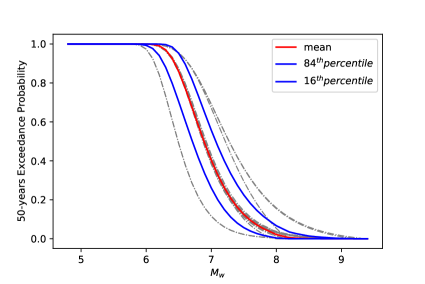
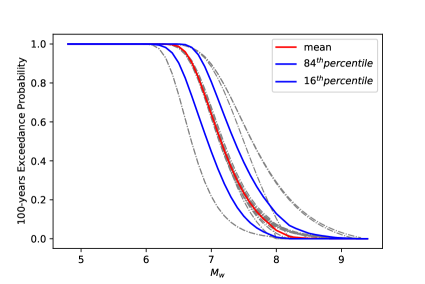
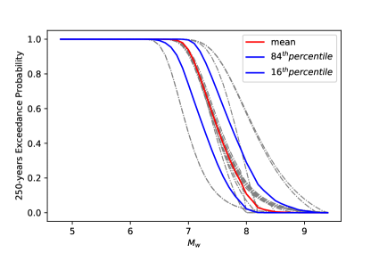
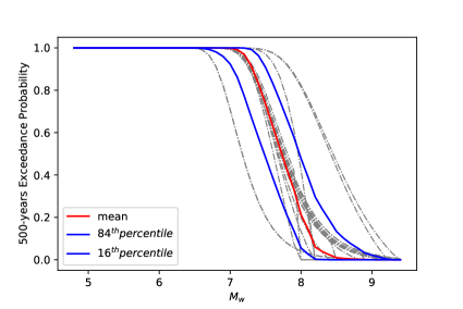
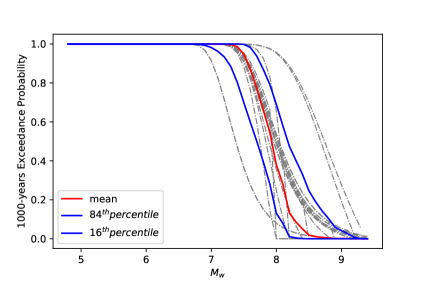
Figure 7: Earthquake probability of exceedance for our sample of $\Delta T$s: red and blue curves show the statistical description of ensemble model, i.e., mean and $16$th-$86$th percentiles, respectively. For comparison, all outcomes of the EV1 branches are also displayed in light gray.

3.2 Tsunami probability exceedance curves

Using the equations described in section 2.5, we calculated the probability of exceedance from a set of tsunami height thresholds $\psi_{t}=\{0.5,1,1.5,..,11.5,12\}$ m and generated hazard curves at different PoIs incorporating all uncertainties described in the previous sections. The results are given in Fig. 8. The hazard curves for each PoI are shown in gray. The results show that the spread of hazard curves for different locations of the Makran coast is remarkably large. As an example, $P^{\text{tot}}(\psi>3,\Delta T=50)$ ranges from $0$ to $13.5\%$ for different PoIs. By increasing $\Delta T$, this range opens up and it reaches $25\%,52\%,74\%$, and $91\%$ for the return periods of 100, 250, 500, and 1000 years, respectively. It is thus not wise to consider a mean (or percentile) of PoI hazard curves for any purpose in the coasts of Iran and Pakistan. Hence, we selected six main PoIs close to the major cities of the Makran region, namely, Chabahar, Konarak, Jask, Ramin, Jiwani, and Gwadar, to explore the results in detail.

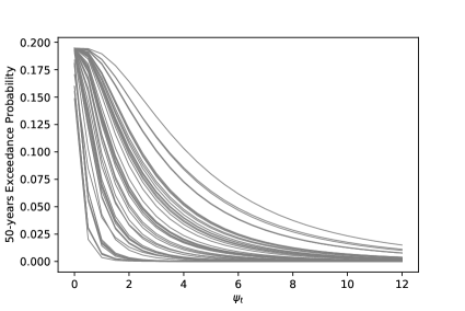
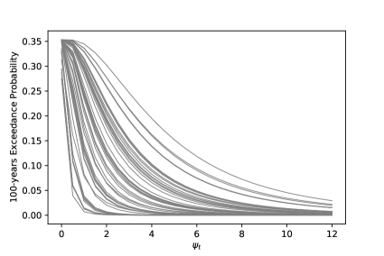
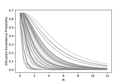
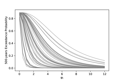
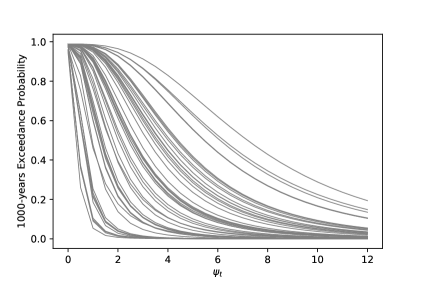
Figure 8: Tsunami probability of exceedance for a sample of $\Delta T$s at different PoIs along the Iran and Pakistan coasts.

Fig. 9 shows the tsunami probability exceedance curve at the above mentioned six major cities for different return periods. For a 50-year return period, the probability of exceedance does not vary much among different cities. However, this difference becomes significant with increasing $\Delta T$. For instance, for $P^{\text{tot}}(\psi>1,\Delta T=1000)$, it ranges from $26\%$ in the west (Gwadar) to $94\%$ in the east (Jask). Moreover, the probability that tsunami height exceeds 4 m is low (less than $10\%$) near all major cities except for Jask, with the probability of $53\%$.

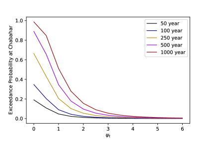
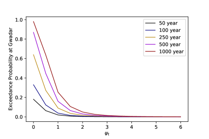
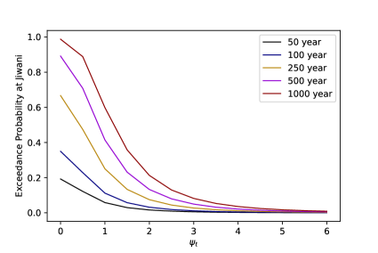
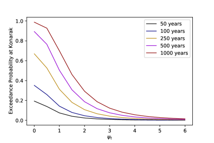
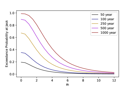
Figure 9: Tsunami probability of the selected $\Delta T$s exceedance for the selected six PoIs near main cities.

3.3 Sensitivity analysis

The effect of inclusion of the aleatory variability introduced in section 2.1.2 is shown in Fig. 10. Fig. 10 (a) illustrates the probability of exceedance in the presence and absence of the aleatory variability at one random PoI (i.e., Chabahar) for two return periods (100 and 500 years). The inclusion of the aleatory variability has a significant effect on the probability of exceedance, which increases for a longer return period. As an example, the differences between $P^{\text{tot}}(\psi>1,\Delta T,\text{Chabahar})$ with and without the aleatory variability are $8\%$ and $26\%$ for $\Delta T=100$ and $500$ years, respectively. To obtain a better interpretation, we also calculated this difference for all PoIs and $\Delta T$s, see Fig. 10 (b). In summary, omitting the aleatory variability mostly leads to a noticeable underestimation with a median of $10\%$ for all PoIs, reaching and it even reaches $40\%$ at somewhere for 1000-year return period.

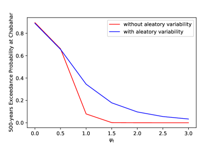
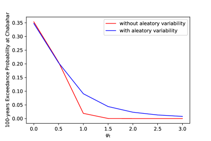
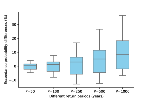
(a)

(b)

Figure 10: (a) Exceedance curve of Chabahar as a random PoI for 100- and 500-year return periods; blue and red curves show the probability of exceedance in the presence and absence of the aleatory variability, respectively; (b) box plot showing the differences in exceedance probability ($\%$) for different $\Delta T$s with and without the presence of the aleatory variability for all PoIs.

3.4 Probability maps

We used a probability map to assess hazard along the entire coast irrespective of population density, which is crucial for prioritizing tsunami mitigation plans and city development in low-population areas. Most literature and mitigation plans focus on specific populated areas (e.g., (Akbarpour Jannat et al., 2017; Payande et al., 2015). Fig. 11 illustrates tsunami probability maps exceeding from two selective thresholds, $\psi_{t}=1,3$ m with different return periods. The probability of exceedance is much more intense in the west. Furthermore, in some rural areas (e.g., Tis and Tang) neighboring Chabahar, the probability that tsunami height will exceed 3 m for return periods of 100 and 1000 years is approximately $25\%$ and $89\%$, respectively. Notably, this is almost $6$ to $7$ times higher than that in Chabahar. Owing to the small distances between these regions, the inundated area at Chabahar may be affected. Inundation maps are beyond the scope of this study, and we plan to address them in a future work.

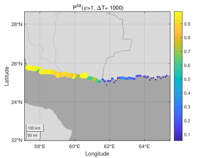
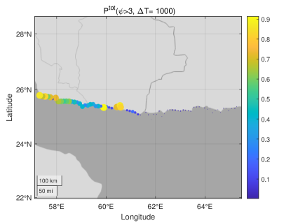
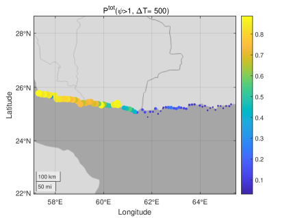
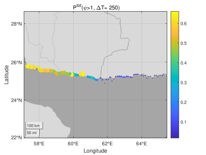
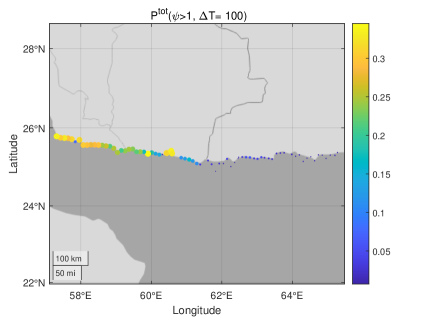
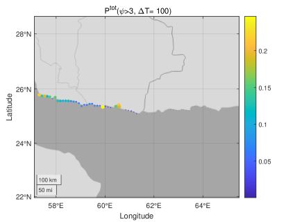
Figure 11: Maps of tsunami probability exceeding 1 and 3 m for different $\Delta T$s along the entire coast of Iran and Pakistan.

4 Conclusions

The MSZ is one of the two sources of tsunamis in the Indian Ocean, and has the potential of generating large tsunamis that threaten neighboring countries of Iran, Oman, and Pakistan. However, a fortune lack of large tsunamis recently has led to a false sense of safety between community leaders and residents, which may negatively affect the area’s vulnerability and resilience against future tsunamis. In addition, a short historical record compared to return period for major subduction zones makes it difficult to conclude the potential risks of future tsunamis. Therefore, in this study, we assessed the potential seismogenic zone, maximum magnitude, and recurrence models at the MSZ using available seismic, geodetic, and historical catalogue data. Moreover, both aleatory and epistemic uncertainties were considered to obtain more accurate and reliable results.

The epistemic uncertainties were incorporated by combining event tree and ensemble modeling, including uncertainties of fault source and rupture complexity (dimensions, slip distribution, and possible locations of earthquakes). The aleatory variability was identified from three main contributions (numerical model and bathymetry, tidal variation, and scaling relation), and incorporated directly into the probability equations, see (10). Our results are demonstrated using hazard curves and probability maps. We also assessed the effect of the aleatory variability. To the best of our knowledge, this is the first PTHA sensitivity analysis concerning aleatory variability in the MSZ. The findings are highlighted as follows.

1. The spread of hazard curves for different locations along the Makran coast is remarkably large. The probability that the tsunami height exceeds 3 m for return periods $\Delta T=\{50,$ $100,250,500,1000\}$ ranges from $0$ to $\{13.5,25,52,74,91\}$ percent, respectively, for different PoIs.

2. The probability of exceedance at PoIs near populated cities decreases and becomes insignificant for the exceedance threshold of 4 m (even for a long return period), except for Jask at the western coast of Iran. Our results provide evidence that if we consider the western part of the MSZ equally active and potential to the eastern part –similar to this paper, by weighting both parts the same in our event tree–the exceedance probability could be higher at the western part for a long return period. This can be clearly seen from the probability maps where the exceedance probability of 3 m fluctuates and becomes maximum at the western part of the MSZ.

3. The inclusion of the aleatory variability has a significant effect on the probability of exceedance, and not including it mostly leads to a remarkable underestimation in the PTHA with a median of $10\%$ difference for all PoIs. This difference is underscored by increasing the return periods and reaches $40\%$ at somewhere for 1000-year return period in the presence and absence of the aleatory variability.

Owing to Makran’s economical, geographical, and strategic importance, Iran approved a plan for developing the southern Makran Coast on December, 2016 titled “Makran Sustainable Development.” This plan, along with the drought occurring recently in the neighboring cities, has led to an inevitable migration toward the coastlines, with Chabahar exhibiting $10\%$ population rate growth last year and ranking among the highest population growth rates globally in 2019. Hence, our results are of vital for various stakeholders for developing and implementing tsunami risk mitigation activities and guiding risk-aware city planning.

This study is the first step toward comprehensive and reliable mitigation plans and activities; however, it is important to acknowledge its limitations. Tsunami sources beyond earthquakes were not considered in this study. Notably, the only tsunami induced with combination of earthquake and landslide in word history occurred in Makran in 1945. Moreover, in September 2013, a landslide was recorded immediately following an earthquake in the MSZ (Heidarzadeh and Satake, 2014). This highlights the need to consider landslides (Rastgoftar and Soltanpour, 2016) and their combination with earthquakes in future PTHA studies. Moreover, we disregarded the dynamic interaction between tides and tsunami waves. This works for a tsunami wave with one isolated peak; however, it may lead to hazard underestimation when the tsunami has several peaks with significant heights. Finally, the necessity and incorporation of high quality bathymetry and topography data is paramount, especially, for mapping tsunami inundation and vulnerable areas, which is the aim of our next study.

Conflicts of interests

The authors have no conflicts of interest to declare that are relevant to the content of this article.

References

- Aida (1978) Aida I (1978) Reliability of a tsunami source model derived from fault parameters. Journal of Physics of the Earth 26(1):57–73
- Akbari et al. (2017) Akbari P, Sadrinasab M, Chegini V, Siadat Mousavi S (2017) Study of tidal components amplitude distribution in the persian gulf, gulf of oman and arabian sea using numerical simulation. Journal of Marine Science and Technology 16(3):27–41
- Akbarpour Jannat et al. (2017) Akbarpour Jannat MR, Rastgoftar E, Asano T (2017) Tsunami assessment for inundation risk management at chabahar bay facilities in iran. International Journal of Coastal and Offshore Engineering 1(2):27–39
- Al-Lazki et al. (2014) Al-Lazki AI, Al-Damegh KS, El-Hadidy SY, Ghods A, Tatar M (2014) Pn-velocity structure beneath arabia–eurasia zagros collision and makran subduction zones. Geological Society, London, Special Publications 392(1):45–60
- Aldama-Bustos et al. (2009) Aldama-Bustos G, Bommer J, Fenton C, Stafford P (2009) Probabilistic seismic hazard analysis for rock sites in the cities of abu dhabi, dubai and ra’s al khaymah, united arab emirates. Georisk 3(1):1–29
- Allen et al. (2012) Allen TI, Wald DJ, Worden CB (2012) Intensity attenuation for active crustal regions. Journal of seismology 16(3):409–433
- Ambraseys and Melville (1982) Ambraseys N, Melville C (1982) A history of persian earthquakes cambridge univ. Press, New York
- Annaka et al. (2007) Annaka T, Satake K, Sakakiyama T, Yanagisawa K, Shuto N (2007) Logic-tree approach for probabilistic tsunami hazard analysis and its applications to the japanese coasts. In: Tsunami and its hazards in the Indian and Pacific Oceans, Springer, pp 577–592
- Berryman et al. (2015) Berryman K, Wallace L, Hayes G, Bird P, Wang K, Basili R, Lay T, Pagani M, Stein R, Sagiya T, et al. (2015) The gem faulted earth subduction interface characterisation project, version 2.0, april 2015. Global Earthquake Model
- Bird and Kagan (2004) Bird P, Kagan YY (2004) Plate-tectonic analysis of shallow seismicity: Apparent boundary width, beta, corner magnitude, coupled lithosphere thickness, and coupling in seven tectonic settings. Bulletin of the Seismological Society of America 94(6):2380–2399
- Blaser et al. (2010) Blaser L, Krüger F, Ohrnberger M, Scherbaum F (2010) Scaling relations of earthquake source parameter estimates with special focus on subduction environment. Bulletin of the Seismological Society of America 100(6):2914–2926
- Bommer and Abrahamson (2006) Bommer JJ, Abrahamson NA (2006) Why do modern probabilistic seismic-hazard analyses often lead to increased hazard estimates? Bulletin of the Seismological Society of America 96(6):1967–1977
- Butler et al. (2017) Butler R, Walsh D, Richards K (2017) Extreme tsunami inundation in hawai ‘i from aleutian–alaska subduction zone earthquakes. Natural Hazards 85(3):1591–1619
- Cornell (1968) Cornell CA (1968) Engineering seismic risk analysis. Bulletin of the seismological society of America 58(5):1583–1606
- Davies (2019) Davies G (2019) Tsunami variability from uncalibrated stochastic earthquake models: tests against deep ocean observations 2006–2016. Geophysical Journal International 218(3):1939–1960
- Davies and Griffin (2019) Davies G, Griffin J (2019) Sensitivity of probabilistic tsunami hazard assessment to far-field earthquake slip complexity and rigidity depth-dependence: Case study of australia. Pure and Applied Geophysics pp 1–28
- Davies et al. (2015) Davies G, Horspool N, Miller V (2015) Tsunami inundation from heterogeneous earthquake slip distributions: Evaluation of synthetic source models. Journal of Geophysical Research: Solid Earth 120(9):6431–6451
- Davies et al. (2018) Davies G, Griffin J, Løvholt F, Glimsdal S, Harbitz C, Thio HK, Lorito S, Basili R, Selva J, Geist E, et al. (2018) A global probabilistic tsunami hazard assessment from earthquake sources. Geological Society, London, Special Publications 456(1):219–244
- Deif and El-Hussain (2012) Deif A, El-Hussain I (2012) Seismic moment rate and earthquake mean recurrence interval in the major tectonic boundaries around oman. Journal of Geophysics and Engineering 9(6):773–783
- Department] (2007) Department] PPM (2007) Seismic hazard analysis and zonation for pakistan, azad jammu and kashmir
- Downes and Stirling (2001) Downes GL, Stirling MW (2001) Groundwork for development of a probabilistic tsunami hazard model for new zealand. In: International Tsunami Symposium 2001, Pacific Marine Environmental Lab. Seattle, Wash., pp 293–301
- El-Hussain et al. (2016) El-Hussain I, Omira R, Deif A, Al-Habsi Z, Al-Rawas G, Mohamad A, Al-Jabri K, Baptista MA (2016) Probabilistic tsunami hazard assessment along oman coast from submarine earthquakes in the makran subduction zone. Arabian Journal of Geosciences 9(15):668
- Frohling and Szeliga (2016) Frohling E, Szeliga W (2016) Gps constraints on interplate locking within the makran subduction zone. Geophysical Supplements to the Monthly Notices of the Royal Astronomical Society 205(1):67–76
- Fujii et al. (2011) Fujii Y, Satake K, Sakai S, Shinohara M, Kanazawa T (2011) Tsunami source of the 2011 off the pacific coast of tohoku earthquake. Earth, planets and space 63(7):55
- Geist and Lynett (2014) Geist EL, Lynett PJ (2014) Source processes for the probabilistic assessment of tsunami hazards. Oceanography 27(2):86–93
- Goda et al. (2014) Goda K, Mai PM, Yasuda T, Mori N (2014) Sensitivity of tsunami wave profiles and inundation simulations to earthquake slip and fault geometry for the 2011 tohoku earthquake. Earth, Planets and Space 66(1):105
- Goda et al. (2019) Goda K, Mori N, Yasuda T, Prasetyo A, Muhammad A, Tsujio D (2019) Cascading geological hazards and risks of the 2018 sulawesi indonesia earthquake and sensitivity analysis of tsunami inundation simulations. Frontiers in Earth Science 7:261
- Grezio et al. (2017) Grezio A, Babeyko A, Baptista MA, Behrens J, Costa A, Davies G, Geist EL, Glimsdal S, González FI, Griffin J, et al. (2017) Probabilistic tsunami hazard analysis: Multiple sources and global applications. Reviews of Geophysics 55(4):1158–1198
- Hayes et al. (2018) Hayes GP, Moore GL, Portner DE, Hearne M, Flamme H, Furtney M, Smoczyk GM (2018) Slab2, a comprehensive subduction zone geometry model. Science 362(6410):58–61
- Heidarzadeh and Kijko (2011) Heidarzadeh M, Kijko A (2011) A probabilistic tsunami hazard assessment for the makran subduction zone at the northwestern indian ocean. Natural hazards 56(3):577–593
- Heidarzadeh and Satake (2014) Heidarzadeh M, Satake K (2014) Possible sources of the tsunami observed in the northwestern indian ocean following the 2013 september 24 m w 7.7 pakistan inland earthquake. Geophysical Journal International 199(2):752–766
- Heidarzadeh and Satake (2017) Heidarzadeh M, Satake K (2017) A combined earthquake–landslide source model for the tsunami from the 27 november 1945 m w 8.1 makran earthquake. Bulletin of the Seismological Society of America 107(2):1033–1040
- Heidarzadeh et al. (2009) Heidarzadeh M, Pirooz MD, Zaker NH (2009) Modeling the near-field effects of the worst-case tsunami in the makran subduction zone. Ocean Engineering 36(5):368–376
- Hoechner et al. (2016) Hoechner A, Babeyko AY, Zamora N (2016) Probabilistic tsunami hazard assessment for the makran region with focus on maximum magnitude assumption. Natural Hazards and Earth System Sciences (NHESS) 16:1339–1350
- Kagan (2002) Kagan YY (2002) Seismic moment distribution revisited: I. statistical results. Geophysical Journal International 148(3):520–541
- Kagan and Jackson (2013) Kagan YY, Jackson DD (2013) Tohoku earthquake: A surprise? Bulletin of the Seismological Society of America 103(2B):1181–1194
- Kajiura (1963) Kajiura K (1963) The leading wave of a tsunami. Bulletin of the Earthquake Research Institute, University of Tokyo 41(3):535–571
- Kakar et al. (2015) Kakar D, Naeem G, Usman A, Mengal A, Naderi Beni A, Afarin M, Ghaffari H, Fritz H, Pahlevan F, Okal E, et al. (2015) Remembering the 1945 makran tsunami; interviews with survivors beside the arabian sea. UNESCO-IOC Brochure 1:79
- Kijko (2004) Kijko A (2004) Estimation of the maximum earthquake magnitude, m max. Pure and Applied Geophysics 161(8):1655–1681
- Kijko et al. (2016) Kijko A, Smit A, Sellevoll MA (2016) Estimation of Earthquake Hazard Parameters from Incomplete Data Files. Part III. Incorporation of Uncertainty of Earthquake‐Occurrence Model. Bulletin of the Seismological Society of America 106(3):1210–1222, DOI 10.1785/0120150252, URL https://doi.org/10.1785/0120150252, https://pubs.geoscienceworld.org/bssa/article-pdf/106/3/1210/3668777/1210.pdf
- Kirby et al. (1998) Kirby JT, Wei G, Chen Q, Kennedy AB, Dalrymple RA (1998) Funwave 1.0: fully nonlinear boussinesq wave model-documentation and user’s manual. research report NO CACR-98-06
- Lolli et al. (2014) Lolli B, Gasperini P, Vannucci G (2014) Empirical conversion between teleseismic magnitudes (mb and m s) and moment magnitude (m w) at the global, euro-mediterranean and italian scale. Geophysical Journal International 199(2):805–828
- Lorito et al. (2015) Lorito S, Selva J, Basili R, Romano F, Tiberti M, Piatanesi A (2015) Probabilistic hazard for seismically induced tsunamis: accuracy and feasibility of inundation maps. Geophysical Journal International 200(1):574–588
- Løvholt et al. (2012) Løvholt F, Pedersen G, Bazin S, Kühn D, Bredesen RE, Harbitz C (2012) Stochastic analysis of tsunami runup due to heterogeneous coseismic slip and dispersion. Journal of Geophysical Research: Oceans 117(C3)
- Løvholt et al. (2014) Løvholt F, Setiadi NJ, Birkmann J, Harbitz CB, Bach C, Fernando N, Kaiser G, Nadim F (2014) Tsunami risk reduction–are we better prepared today than in 2004? International journal of disaster risk reduction 10:127–142
- Løvholt et al. (2015) Løvholt F, Griffin J, Salgado-Gálvez M (2015) Tsunami hazard and risk assessment on the global scale. Encyclopedia of complexity and systems science pp 1–34
- Lynett et al. (2016) Lynett P, Wei Y, Arcas DR (2016) Tsunami Hazard Assessment: Best Modeling Practices and State-of-the Art Technology. United States Nuclear Regulatory Commission, Office of Nuclear Regulatory …
- Marzocchi et al. (2015) Marzocchi W, Taroni M, Selva J (2015) Accounting for epistemic uncertainty in psha: Logic tree and ensemble modeling. Bulletin of the Seismological Society of America 105(4):2151–2159
- Mori et al. (2018) Mori N, Goda K, Cox D (2018) Recent process in probabilistic tsunami hazard analysis (ptha) for mega thrust subduction earthquakes. In: The 2011 Japan Earthquake and Tsunami: Reconstruction and Restoration, Springer, pp 469–485
- Mueller et al. (2015) Mueller C, Power W, Fraser S, Wang X (2015) Effects of rupture complexity on local tsunami inundation: Implications for probabilistic tsunami hazard assessment by example. Journal of Geophysical Research: Solid Earth 120(1):488–502
- Mulia et al. (2020) Mulia IE, Ishibe T, Satake K, Gusman AR, Murotani S (2020) Regional probabilistic tsunami hazard assessment associated with active faults along the eastern margin of the sea of japan. Earth, Planets and Space 72(1):1–15
- Normand et al. (2019) Normand R, Simpson G, Herman F, Biswas RH, Bahroudi A (2019) Holocene sedimentary record and coastal evolution in the makran subduction zone (iran). Quaternary 2(2):21
- Okada (1985) Okada Y (1985) Surface deformation due to shear and tensile faults in a half-space. Bulletin of the seismological society of America 75(4):1135–1154
- Okal et al. (2015) Okal EA, Fritz HM, Hamzeh MA, Ghasemzadeh J (2015) Field survey of the 1945 makran and 2004 indian ocean tsunamis in baluchistan, iran. Pure and Applied Geophysics 172(12):3343–3356
- Payande et al. (2015) Payande A, Niksokhan M, Naserian H (2015) Tsunami hazard assessment of chabahar bay related to megathrust seismogenic potential of the makran subduction zone. Natural hazards 76(1):161–176
- Power et al. (2012) Power W, Wallace L, Wang X, Reyners M (2012) Tsunami hazard posed to new zealand by the kermadec and southern new hebrides subduction margins: an assessment based on plate boundary kinematics, interseismic coupling, and historical seismicity. Pure and applied geophysics 169(1-2):1–36
- Rastgoftar and Soltanpour (2016) Rastgoftar E, Soltanpour M (2016) Study and numerical modeling of 1945 makran tsunami due to a probable submarine landslide. Natural Hazards 83(2):929–945
- Reasenberg (1985) Reasenberg P (1985) Second-order moment of central california seismicity, 1969–1982. Journal of Geophysical Research: Solid Earth 90(B7):5479–5495
- Reyes and Wiemer (2019) Reyes C, Wiemer S (2019) Zmap7, a refreshed software package to analyze seismicity. In: Geophysical Research Abstracts, vol 21
- Rikitake and Aida (1988) Rikitake T, Aida I (1988) Tsunami hazard probability in japan. Bulletin of the Seismological Society of America 78(3):1268–1278
- Safari et al. (2017) Safari A, Abolghasem A, Abedini N, Mousavi Z (2017) Assessment of optimum value for dip angle and locking rate parameters in makran subduction zone. International Archives of the Photogrammetry, Remote Sensing & Spatial Information Sciences 42
- Salah and Soltanpour (2014) Salah P, Soltanpour M (2014) Modeling of tsunami propagation and inundation at the north coast of gulf of oman due to earthquake in makran subduction zone. International conference on coasts, ports and marine structures (icopmas) 11
- Satake (2014) Satake K (2014) Advances in earthquake and tsunami sciences and disaster risk reduction since the 2004 indian ocean tsunami. Geoscience Letters 1(1):15
- Shi et al. (2012) Shi F, Kirby JT, Harris JC, Geiman JD, Grilli ST (2012) A high-order adaptive time-stepping tvd solver for boussinesq modeling of breaking waves and coastal inundation. Ocean Modelling 43:36–51
- Smith et al. (2013) Smith GL, McNeill LC, Wang K, He J, Henstock TJ (2013) Thermal structure and megathrust seismogenic potential of the makran subduction zone. Geophysical Research Letters 40(8):1528–1533
- Starrs (2014) Starrs R (2014) When the tsunami came to shore: Culture and disaster in Japan. Global Oriental
- Strasser et al. (2010) Strasser FO, Arango M, Bommer JJ (2010) Scaling of the source dimensions of interface and intraslab subduction-zone earthquakes with moment magnitude. Seismological Research Letters 81(6):941–950
- Sugino et al. (2015) Sugino H, Iwabuchi Y, Hashimoto N, Matsusue K, Ebisawa K, Kameda H, Imamura F (2015) The characterizing model for tsunami source regarding the inter-plate earthquake tsunami. Journal of JAEE 15(3):3_114–3_133
- Tajalli Bakhsh (2014) Tajalli Bakhsh T (2014) Improvements and applications of state-of-the-art numerical models for simulating tsunami hazard. PhD thesis
- Tehranirad et al. (2011) Tehranirad B, Shi F, Kirby JT, Harris JC, Grilli S (2011) Tsunami benchmark results for fully nonlinear boussinesq wave model funwave-tvd, version 1.0. Center for Applied Coastal Research, University of Delaware, Tech Rep
- Thio (2010) Thio HK (2010) Urs probabilistic tsunami hazard system: A user manual. Technical Report URS Corporation, San Francisco, CA
- Thio et al. (2007) Thio HK, Somerville P, Ichinose G (2007) Probabilistic analysis of strong ground motion and tsunami hazards in southeast asia. Journal of Earthquake and Tsunami 1(02):119–137
- Thio et al. (2014) Thio HK, Wilson RI, Miller K (2014) Evaluation and application of probabilistic tsunami hazard analysis in california. AGUFM 2014:NH12A–01
- Ward et al. (2020) Ward PJ, Blauhut V, Bloemendaal N, Daniell JE, de Ruiter MC, Duncan MJ, Emberson R, Jenkins SF, Kirschbaum D, Kunz M, et al. (2020) Natural hazard risk assessments at the global scale. Natural Hazards and Earth System Sciences 20(4)