Efficient Robust Training via Backward Smoothing

Abstract

Adversarial training is so far the most effective strategy in defending against adversarial examples. However, it suffers from high computational costs due to the iterative adversarial attacks in each training step. Recent studies show that it is possible to achieve fast Adversarial Training by performing a single-step attack with random initialization. However, such an approach still lags behind state-of-the-art adversarial training algorithms on both stability and model robustness. In this work, we develop a new understanding towards Fast Adversarial Training, by viewing random initialization as performing randomized smoothing for better optimization of the inner maximization problem. Following this new perspective, we also propose a new initialization strategy, backward smoothing, to further improve the stability and model robustness over single-step robust training methods. Experiments on multiple benchmarks demonstrate that our method achieves similar model robustness as the original TRADES method while using much less training time ($\sim$3x improvement with the same training schedule).

1 Introduction

Deep neural networks are well known to be vulnerable to adversarial examples (Szegedy et al. 2013), i.e., a small perturbation on the original input can lead to misclassification or erroneous prediction. Many defense methods have been developed to mitigate the disturbance of adversarial examples (Guo et al. 2018; Xie et al. 2018; Song et al. 2018; Ma et al. 2018; Samangouei, Kabkab, and Chellappa 2018; Dhillon et al. 2018; Madry et al. 2018; Zhang et al. 2019), among which robust training methods, such as adversarial training (Madry et al. 2018) and TRADES (Zhang et al. 2019), are currently the most effective strategies. Specifically, adversarial training method (Madry et al. 2018) trains a model on adversarial examples by solving a min-max optimization problem:

$$\min_{\bm{\theta}}\frac{1}{n}\sum_{i=1}^{n}\max_{\mathbf{x}_{i}^{\prime}\in\mathcal{B}_{\epsilon}(\mathbf{x}_{i})}L(f_{\bm{\theta}}(\mathbf{x}_{i}^{\prime}),y_{i}),$$ (1.1)

where $\{(\mathbf{x}_{i},y_{i})\}_{i=1}^{n}$ is the training dataset, $f(\cdot)$ denotes the logits output of the neural network, $\mathcal{B}_{\epsilon}(\mathbf{x}_{i}):=\{\mathbf{x}:\|\mathbf{x}-\mathbf{x}_{i}\|_{\infty}\leq\epsilon\}$ denotes the $\epsilon$-perturbation ball, and $L$ is the cross-entropy loss.

On the other hand, instead of directly training on adversarial examples, TRADES (Zhang et al. 2019) further improves model robustness with a trade-off between natural accuracy and robust accuracy, by solving the empirical risk minimization problem with a robust regularization term:

$$\min_{\bm{\theta}} \frac{1}{n}\sum_{i=1}^{n}\Big{[}L(f_{\bm{\theta}}(\mathbf{x}_{i}),y_{i})$$

$$+\beta\max_{\mathbf{x}_{i}^{\prime}\in\mathcal{B}_{\epsilon}(\mathbf{x}_{i})}\text{KL}\big{(}s(f_{\bm{\theta}}(\mathbf{x}_{i})),s(f_{\bm{\theta}}(\mathbf{x}_{i}^{\prime}))\big{)}\Big{]},$$ (1.2)

where $s(\cdot)$ denotes the softmax function, and $\beta>0$ is a regularization parameter. The goal of this robust regularization term (i.e., KL divergence term) is to ensure the outputs are stable within the local neighborhood. Both adversarial training and TRADES achieve good model robustness, as shown on recent model robustness leaderboards (Croce and Hein 2020b; Chen and Gu 2020). However, a major drawback lies in that both are highly time-consuming for training, limiting their usefulness in practice. This is largely due to the fact that both methods perform iterative adversarial attacks (i.e., Projected Gradient Descent) to solve the inner maximization problem in each outer minimization step.

Recently, (Wong, Rice, and Kolter 2020) shows that it is possible to use single-step adversarial attacks to solve the inner maximization problem, which previously was believed impossible. The key ingredient in their Fast AT approach is adding a random initialization step before the single-step adversarial attack. This simple change leads to a reasonably robust model that outperforms other fast robust training techniques, e.g., (Shafahi et al. 2019). However, the simple change also has its downsides: 1) random initialization makes single-step robust training possible yet it can be quite unstable (Li et al. 2020); 2) compared to state-of-the-art robust training models (Madry et al. 2018; Zhang et al. 2019), Fast AT still lags behind on model robustness. Besides these, It also remains a mystery in (Wong, Rice, and Kolter 2020) on why random initialization is empirically effective.

Although some attempts have been made trying to explain the role of random initialization and further improve Fast AT (Andriushchenko and Flammarion 2020; Li et al. 2020), in this work, we aim to understand the role of random initialization in (Wong, Rice, and Kolter 2020) from a new perspective and further improve the model robustness-efficiency trade-off over previous fast robust training methods. Specifically, We propose a new principle towards understanding Fast AT - that random initialization can be viewed as performing randomized smoothing for better optimization of the inner maximization problem. In order to further improve the robustness-efficiency trade-off of fast robust training techniques, we propose a new initialization strategy, backward smoothing, which strengthens the smoothing effect within the $\epsilon$-perturbation ball. The resulting method significantly improves both stability and model robustness over the single-step random initialization strategies. Moreover, even comparing with full-step robust training methods such as TRADES (Zhang et al. 2019), our proposed backward smoothing strategy achieves similar model robustness while consuming much less training time ($\sim 3$x improvement with the same training schedule).

The remainder of this paper is organized as follows: in Section 2, we briefly review existing literature on adversarial attacks, robust training as well as randomized smoothing technique. We present our new understanding of random initialization in Section 3. We present our proposed method in Section 4. In Section 5, we empirically evaluate our proposed method with other state-of-the-art baselines. Finally, we conclude this paper in Section 6.

2 Related Work

There exists a large body of literature on adversarial attacks and defenses. In this section, we only review the most relevant work to ours.

Adversarial Attack  The concept of adversarial examples was first proposed in (Szegedy et al. 2013). Since then, many methods have been proposed, such as Fast Gradient Sign Method (FGSM) (Goodfellow, Shlens, and Szegedy 2015), and Projected Gradient Descent (PGD) (Kurakin, Goodfellow, and Bengio 2016; Madry et al. 2018). Later on, various attacks (Papernot et al. 2016; Moosavi-Dezfooli, Fawzi, and Frossard 2016; Carlini and Wagner 2017; Athalye, Carlini, and Wagner 2018; Chen et al. 2020; Croce and Hein 2020a; Sriramanan et al. 2020; Tashiro, Song, and Ermon 2020) were also proposed for better effectiveness or efficiency.

There are also many attacks focused on different attack settings. (Chen et al. 2017) proposed a black-box attack where the gradient is not available, by estimating the gradient via finite-differences. Various methods (Ilyas et al. 2018; Al-Dujaili and O’Reilly 2020; Moon, An, and Song 2019; Andriushchenko et al. 2020; Tashiro, Song, and Ermon 2020) have been developed to improve the query efficiency of (Chen et al. 2017). Other methods (Brendel, Rauber, and Bethge 2018; Cheng et al. 2019, 2020) focused on the more challenging hard-label attack setting, where only the prediction labels are available. On the other hand, there is recent work (Croce and Hein 2020b; Chen and Gu 2020) that aims to accurately evaluate the model robustness via an ensemble of attacks or effective hard-label attack.

Robust Training  Many heuristic defenses (Guo et al. 2018; Xie et al. 2018; Song et al. 2018; Ma et al. 2018; Samangouei, Kabkab, and Chellappa 2018; Dhillon et al. 2018) were proposed when the concept of adversarial examples was first introduced. However, they are later shown by (Athalye, Carlini, and Wagner 2018) as not truly robust. Adversarial training (Madry et al. 2018) is the first effective method towards defending against adversarial examples. Various adversarial training variants (Wang et al. 2019, 2020; Zhang et al. 2019; Wu, Xia, and Wang 2020; Sriramanan et al. 2020; Zhang et al. 2020) were later proposed to further improve the adversarially trained model robustness. A line of researches focus on studying various others factors affecting model robustness such as early-stopping (Rice, Wong, and Kolter 2020), model width (Wu et al. 2021), loss landscape (Liu et al. 2020) and parameter tuning (Pang et al. 2021; Gowal et al. 2020). Another line of research utilizes extra information (e.g., pre-trained models (Hendrycks, Lee, and Mazeika 2019) or extra unlabeled data (Carmon et al. 2019; Alayrac et al. 2019)) to further improve robustness.

Recently, many focus on improving the training efficiency of adversarial training based algorithms, such as free adversarial training (Shafahi et al. 2019) and Fast AT (Wong, Rice, and Kolter 2020), which uses single-step attack (FGSM) with random initialization. (Li et al. 2020) proposed a hybrid approach for improving Fast AT which is orthogonal to ours. (Andriushchenko and Flammarion 2020) proposed a new regularizer promoting gradient alignment for more stable training. Yet, its model robustness still falls behind the state-of-the-arts.

Randomized Smoothing  (Duchi, Bartlett, and Wainwright 2012) proposed the randomized smoothing technique and proved variance-based convergence rates for non-smooth optimization. Later on, this technique was applied to certified adversarial defenses (Cohen, Rosenfeld, and Kolter 2019; Salman et al. 2019) for building robust models with certified robustness guarantees. In this paper, we are not targeting certified defenses. Instead, we use the randomized smoothing concept in optimization to explain Fast AT.

3 Pros and Cons of Random Initialization

In this section, we analyze the pros and cons of random initialization in Fast AT (Wong, Rice, and Kolter 2020). First, let us explain why random initialization in Fast AT is effective by looking into why one-step AT would fail without random initialization.

What Caused the Failure of One-step AT Without Random Initialization?

(Wong, Rice, and Kolter 2020) has already shown that without random initialization, one-step AT would almost surely fail in the training procedure due to catastrophic overfitting, i.e., the robust accuracy w.r.t. a PGD adversarial suddenly drops to near $0$ even on training data. However, it is not clear what exactly causes this phenomenon. One natural conjecture is that perhaps the one-step attack is not effective enough for adversarial training purposes. Recall that the perturbation is obtained by solving the following inner maximization problem in adversarial training:

$$\bm{\delta}^{*}=\mathop{\mathrm{argmax}}_{\bm{\delta}\in\mathcal{B}_{\epsilon}({\bm{0}})}L(f_{\bm{\theta}}(\mathbf{x}+\bm{\delta}),y).$$ (3.1)

To figure out whether the attack effectiveness is the key cause for the poor performance of the plain one-step AT without random initialization, we conduct the following simple experiments by observing the loss increment after attack in each training step, i.e.,

$$\Delta_{L}=L(f_{\bm{\theta}}(\mathbf{x}+\bm{\delta}^{*}),y)-L(f_{\bm{\theta}}(\mathbf{x}),y),$$

where $\{(\mathbf{x},y)\}$ is the clean training example and $\bm{\delta}^{*}$ is the solution from (3.1). Since (3.1) aims at maximizing the loss value, this loss increment term $\Delta_{L}$ should always be positive along the entire training trajectory.

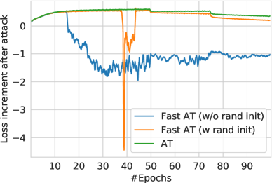
Figure 1: Loss increment after attack, i.e., $L(f_{\bm{\theta}}(\mathbf{x}+\bm{\delta}^{*}),y)-L(f_{\bm{\theta}}(\mathbf{x}),y)$, along the training trajectory for different methods on training ResNet-18 on CIFAR-10 dataset.

In Figure 1, we plot the loss increment $\Delta_{L}$ for three different training trajectories: Fast AT without random initialization, Fast AT with random initialization, as well as standard AT. We observe that with the random initialization, Fast AT’s loss increment is quite close to standard AT (although it still can go wrong from time to time). However, without random initialization, the loss value after the attack is actually worse than before, suggesting the algorithm completed failed in solving (3.1). Since Fast AT has only one step budget for the attack, this further implies the attack step size is too large to cause divergence in the gradient descent procedure. Yet on the other hand, due to the one step attack budget, the attack step size has to be chosen close to $\epsilon$ for better defense purposes. This dilemma explains the cause of failure for one-step AT without random initialization.

Why Random Initialization Helps?

Now let us talk about random initialization. It is well known from optimization theory (Boyd, Boyd, and Vandenberghe 2004) that, for gradient descent-based algorithms, the maximum allowed step size (in order to guarantee convergence) is directly related to the smoothness of the optimization objective function. Specifically, the smoother the objective function is, the larger the gradient step size is allowed. Here we argue that random initialization works just as the randomized smoothing technique (Duchi, Bartlett, and Wainwright 2012), which makes the overall optimization objective more smooth via random perturbations of the optimization variable. Note that this randomized smoothing is an optimization technique that is different from the Randomized Smoothing method in certified defenses (Cohen, Rosenfeld, and Kolter 2019), although the names are the same.

To see why random initialization works as randomized smoothing in Fast AT, let us apply randomized smoothing to (3.1) and we have:

$$\bm{\delta}^{*}=\mathop{\mathrm{argmax}}_{\bm{\delta}+u\bm{\xi}\in\mathcal{B}_{\epsilon}(\bm{0})}\mathbb{E}_{\bm{\xi}\sim U(-1,1)}L(f_{\bm{\theta}}(\mathbf{x}+\bm{\delta}+u\bm{\xi}),y),$$ (3.2)

where $\bm{\xi}$ is the perturbation vector for randomized smoothing, $u$ controls the smoothing effect, and $\bm{\delta}$ is the adversarial perturbation vector (initialized as zero). Suppose we have $u=\epsilon$ and solve (3.2) in a stochastic fashion (i.e., sample a random perturbation $\bm{\xi}$ instead of computing the expectation over $\bm{\xi}$), and using only one step gradient update, it reduces to the Fast AT formulation. This suggests that Fast AT can be viewed as performing stochastic single-step attacks on a randomized smoothed objective function which allows the use of larger step size. This explains why random initialization helps Fast AT in Figure 1: as it makes the loss objective smoother, thus become easier to optimize with large step sizes and avoid possible divergence cases.

It is worth noting that (Andriushchenko and Flammarion 2020) also provided an explanation of random initialization: it reduces the magnitude of the perturbation and thus the network becomes more linear and fits better toward single-step attack. In fact, our argument is more general and can cover theirs, because if the loss function is approximately linear, then it will be very smooth, i.e., the second-order term in the Taylor expansion is small. And their observations that Fast AT using smaller attack step size can succeed without random initialization actually also validate our analysis above.

Drawbacks of Random Initialization

Although the random initialization effectively helps Fast AT avoid the catastrophic overfitting from happening in the most time, it still exposes several major weaknesses.

Performance Stability  Fast AT can still be highly unstable (i.e., catastrophic overfitting can still occur from time to time). This is also observed in (Li et al. 2020). In Figure 1, we also observe that Fast AT could still fail in solving the inner maximization problem (especially when using a drastically large attack step size). It can be imagined that with some bad luck, the training procedure of Fast AT could still fall apart even with random initialization.

Unfortunately, to get the best from Fast AT, it usually requires a larger attack step size. We run Fast AT on CIFAR-10 using ResNet-18 model (He et al. 2016) for $10$ times. For the best attack step size of $10/255$ (according to (Wong, Rice, and Kolter 2020)), the best run achieves $46.30\%$ robust accuracy, however, the average is only $42.11\%$ since many runs actually failed.

Table 1: Model robustness comparison among AT, Fast AT, TRADES and Fast TRADES, using ResNet-18 model on CIFAR-10 dataset.

Method	Nat (%)	Rob (%)
AT	82.36	51.14
Fast AT	84.79	46.30
TRADES	82.33	52.74
Fast TRADES	83.39	46.98

*Nat: accuracy evaluated on the clean test examples;
*Rob: accuracy evaluated on adversarial examples of the test set.

Further Robustness Improvement  Fast AT uses standard adversarial training (Madry et al. 2018) as the baseline, and can obtain similar robustness performance. However, later work (Rice, Wong, and Kolter 2020) shows that original adversarial training’s performance is deteriorated by robust overfitting, while simply using early stopping can largely improve its robustness. (Zhang et al. 2019) further achieves even better model robustness that is much higher than what Fast AT obtains. From Table 1, we observe that there exists a $6\%$ robust accuracy gap on the CIFAR-10 dataset between Fast AT and TRADES. This indicates that Fast AT is still far from optimal, and there is still big room for further robustness improvement.

4 Proposed Approaches

A Naive Try: Randomized Smoothing for TRADES

In the previous section, we show that objective smoothness plays a key role in the success of single-step adversarial training. Note the TRADES (Zhang et al. 2019) method naturally promotes the objective smoothness in its training formula (by minimizing the output discrepancy of input examples within the perturbation ball). From this perspective, it should be more fit to single-step robust training than AT. Therefore we try to apply randomized smoothing to TRADES and see if this leads to a better robust training method. Let us recall the inner maximization formulation for TRADES:

$$\max_{\bm{\delta}\in\mathcal{B}_{\epsilon}({\bm{0}})}\text{KL}\big{(}s(f_{\bm{\theta}}(\mathbf{x})),s(f_{\bm{\theta}}(\mathbf{x}+\bm{\delta}))\big{)},$$ (4.1)

where $s(\cdot)$ denotes the softmax function. Similarly, we can further apply randomized smoothing technique on this objective and obtain:

$$\max_{\bm{\delta}+u\bm{\xi}\in\mathcal{B}_{\epsilon}(\bm{0})}\mathbb{E}_{\bm{\xi}\sim U(-1,1)}\text{KL}\big{(}s(f_{\bm{\theta}}(\mathbf{x})),s(f_{\bm{\theta}}(\mathbf{x}+\bm{\delta}+u\bm{\xi}))\big{)}.$$ (4.2)

Then we can apply the same stochastic single step attack and $u=\epsilon$ for solving this problem, i.e., first do random initialization and then perform single-step projected gradient ascent on TRADES loss. We refer to this strategy as Fast TRADES. We experimentally test Fast TRADES by training the ResNet-18 model on the CIFAR-10 dataset. From Table 1, we can see that Fast TRADES indeed achieves slightly better performance than Fast AT. Yet it still falls far behind the original TRADES method. This inspires us to study how to design a better strategy for more significant improvements.

Note that our best performing Fast TRADES model in Table 1 is obtained with attack step size $6/255$ (in contrast to $10/255$ for Fast AT). According to our previous analysis in Section 3, if we can make the loss objective even smoother, it is possible to utilize an even larger attack step size for better robust training performances. However, unlike the general randomized smoothing setting, where we can simply use a larger value of $u$ for a smoother objective, in the adversarial setting, the random perturbation on the input vector is subject to the $\epsilon$-ball constraint. This means that simply using larger $u$ cannot bring us a smoother loss objective, instead, we need to find new ways for better smoothing effects.

Backward Smoothing

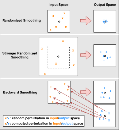
Figure 2: A sketch of our proposed method.

Now we introduce our proposed method to further boost the smoothing effect without violating the $\epsilon$-ball constraint. Let us denote the input domain $\mathbf{x}\in\mathbb{R}^{d}$ as the input space, and their corresponding neural network output $f_{\bm{\theta}}(\mathbf{x})\in\mathbb{R}^{c}$ as the output space, where $c$ is the number of classes for the classifier. Note that if we have random samples in the input space, the corresponding output is actually quite close (Tashiro, Song, and Ermon 2020) as in the first row of Figure 2. Imagine that if we are allowed to use a larger $u$, the output space would be more diverse as in the second row of Figure 2. This inspires us to generate the initialization point in a backward fashion. We first generate random points in the output space just as randomized smoothing does in the input space (see third row of Figure 2, lower right plot), i.e., $f_{\bm{\theta}}(\mathbf{x})+\gamma\bm{\psi}$, where $\bm{\psi}\sim U(-1,1)$ is the random variable and $\gamma$ is a small number. Then we find the corresponding input perturbation in a backward fashion and use it as our initialization. An illustrative sketch of our proposed method is provided in Figure 2. In summary, we aim to find the input perturbation $\bm{\xi}$ such that:

$$f_{\bm{\theta}}(\mathbf{x}+\bm{\xi})=f_{\bm{\theta}}(\mathbf{x})+\gamma\bm{\psi}.$$ (4.3)

In order to find the best $\bm{\xi}^{*}$ to satisfy (4.3), we turn to solve the following problem:

$$\bm{\xi}^{*}=\mathop{\mathrm{argmin}}_{\bm{\xi}\in\mathcal{B}_{\epsilon}(\bm{0})}\text{KL}\big{(}s(f_{\bm{\theta}}(\mathbf{x})+\gamma\bm{\psi}),s(f_{\bm{\theta}}(\mathbf{x}+\bm{\xi}))\big{)}.$$ (4.4)

Note that $\bm{\xi}$ is initialized as a zero vector. For the sake of computational efficiency, we solve (4.4) using single-step PGD in practice. Then, similar to (Wong, Rice, and Kolter 2020), we use single-step gradient update for the inner maximization problem:

$$\bm{\delta}^{*}=\mathop{\mathrm{argmax}}_{\bm{\delta}+\bm{\xi}^{*}\in\mathcal{B}_{\epsilon}(\bm{0})}\text{KL}\big{(}s(f_{\bm{\theta}}(\mathbf{x})),s(f_{\bm{\theta}}(\mathbf{x}+\bm{\delta}+\bm{\xi}^{*}))\big{)}.$$ (4.5)

Finally, we update the neural network parameter $\bm{\theta}$ using stochastic gradients at $\mathbf{x}+\bm{\xi}^{*}+\bm{\delta}^{*}$. A summary of our proposed algorithm is provided in Algorithm 1.

Algorithm 1 Backward Smoothing

1:  input: The number of training iterations $T$, number of adversarial perturbation steps $K$, maximum perturbation strength $\epsilon$, training step size $\eta$, adversarial perturbation step size $\alpha$, regularization parameter $\beta>0$;

2:  Random initialize model parameter $\bm{\theta}_{0}$

3:  for $t=1,\ldots,T$ do

4:     Sample mini-batch $\{\mathbf{x}_{i},y_{i}\}_{i=1}^{m}$ from training set

5:     Obtain $\bm{\xi}^{*}$ by solving (4.4)

6:     Obtain $\bm{\delta}^{*}$ by solving (4.5)

7:     $\bm{\theta}_{t}=\bm{\theta}_{t-1}-\eta/m\cdot\sum_{i=1}^{m}\nabla_{\bm{\theta}}\big{[}L(f_{\bm{\theta}}(\mathbf{x}_{i}),y_{i})+\beta\cdot\text{KL}\big{(}s(f_{\bm{\theta}}(\mathbf{x}_{i})),s(f_{\bm{\theta}}(\mathbf{x}_{i}+\bm{\xi}^{*}+\bm{\delta}^{*}))\big{)}\big{]}$

8:  end for

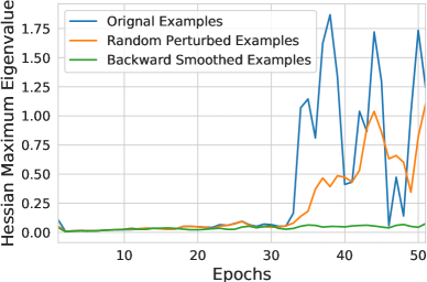
Figure 3: Hessian maximum eigenvalue comparison against training epochs.

Figure 3 shows the maximum eigenvalue of Hessian of the loss function at the original examples, randomly perturbed examples, and backward smoothed examples along the training trajectory until Fast TRADES obtains its best robustness (the 51st epoch). We observe that during the model training process, the randomly perturbed examples have overall smaller Hessian maximum eigenvalue than that of original examples. This suggests that random smoothing indeed makes the loss function smoother. Moreover, the Hessian maximum eigenvalue under backward smoothing is much smaller than that under random smoothing, showing the insufficiency of the random smoothing techniques and the advantages of our proposed backward smoothing method.

5 Experiments

In this section, we empirically evaluate the performance of our proposed method. We first compare our proposed method with other robust training baselines on CIFAR-10, CIFAR100 (Krizhevsky, Hinton et al. 2009) and Tiny ImageNet (Deng et al. 2009) datasets. We also provide multiple ablation studies as well as robustness evaluation with state-of-the-art adversarial attack methods to validate that our proposed method provides effective robustness improvement.

Experimental Setting

Following previous work on robust training (Madry et al. 2018; Zhang et al. 2019; Wong, Rice, and Kolter 2020), we set $\epsilon=0.031$ for all three datasets. In terms of model architecture, we adopt standard ResNet-18 model (He et al. 2016) for both CIFAR-10 and CIFAR-100 datasets, and ResNet-50 model for Tiny ImageNet. We follow the standard piecewise learning rate decay schedule as used in (Madry et al. 2018; Zhang et al. 2019) and set decaying point at $50$-th and $75$-th epochs. The starting learning rate for all methods is set to $0.1$, the same as previous work (Madry et al. 2018; Zhang et al. 2019). For all methods, we tune the models for their best robustness performances for a fair comparison. For Adversarial Training and TRADES methods, we adopt a $10$-step iterative PGD attack with a step size of $2/255$ for both. For our proposed method, we set the backward smoothing parameter $\gamma=1$ and step size as $8/255$. For other fast training methods, we use a step size of $10/255$ for Fast AT/GradAlign, $6/255$ for 2-step Fast AT, $6/255$ for Fast TRADES and $5/255$ for 2-step Fast TRADES. For robust accuracy evaluation, we typically adopt a $100$-step PGD attack with the step size of $2/255$. To ensure the validity of the model robustness improvement is not because of the obfuscated gradient (Athalye, Carlini, and Wagner 2018), we further test our method with current state-of-the-art attacks (Croce and Hein 2020b; Chen and Gu 2020). All the experiments are conducted on RTX2080Ti GPU servers.

Performance Comparison with Robust Training Baselines

We compare the adversarial robustness of Backward Smoothing against standard Adversarial Training (Madry et al. 2018), TRADES (Zhang et al. 2019), as well as fast training methods such as Fast AT (Wong, Rice, and Kolter 2020) and our naive baseline Fast TRADES. We also compare with recently proposed Fast AT+ (Li et al. 2020) and GradAlign (Andriushchenko and Flammarion 2020). Since our proposed backward smoothing initialization utilizes an extra step of gradient back-propagation, we also compare with Fast AT, Fast TRADES using 2-step attack for a fair comparison.

Table 2: Performance comparison on CIFAR-10 using ResNet-18 model.

Method	Nat (%)	Rob (%)	Time (m)
AT	82.36	51.14	430
Fast AT	84.79	46.30	82
Fast AT (2-step)	83.21	49.91	127
Fast AT (GradAlign)	84.37	46.99	402
TRADES	82.33	52.74	482
Fast TRADES	83.39	46.98	126
Fast TRADES (2-step)	83.51	48.78	164
Backward Smoothing	82.38	52.50	164

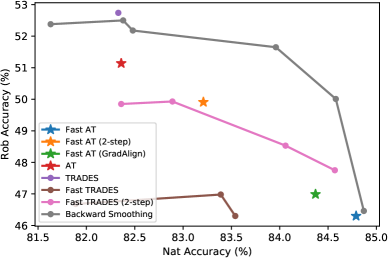
Figure 4: Backward Smoothing’s performance gain is not due to robustness-accuracy trade-off.

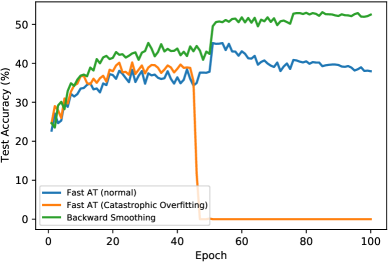
Figure 5: Backward Smoothing does not suffer from the catastrophic overfitting phenomenon.

Table 2 shows the performance comparison on the CIFAR-10 dataset using ResNet-18 model. Our Backward Smoothing method achieves high robust accuracy that is almost as good as state-of-the-art methods such as TRADES, while consuming much less ($\sim$3x) training time. Compared with Fast AT, Backward Smoothing typically costs twice the training time, yet achieving significantly higher model robustness. Notice that the GradAlign method indeed slightly improves upon Fast AT, but it also costs much more training time due to its double backpropagation formulation, making it less competitive to our Backward Smoothing method. Our method also achieves a large performance gain against Fast TRADES. Note that even compared with Fast TRADES using 2-step attack and Fast AT using 2-step attack, which costs about the same training time as ours, our method still achieves a large improvement.

Note that Zhang et al. (2019) has shown that there exists a robustness-accuracy trade-off in robust training. In order to make sure that our proposed method’s performance gain is not due to this robustness-accuracy trade-off, we further test with different choices of robust regularization parameter $\beta$ and plot the robust accuracy against natural accuracy plot in Figure 4. Note that for AT and Fast AT or GradAlign method, their formulations do not contain any tunable parameters for this robustness-accuracy trade-off, therefore, we only plot the single point for them. From Figure 4, we can observe that the Backward Smoothing method indeed largely outperforms the other fast training baselines (achieve better robustness under roughly the same natural accuracy), and is not due to balancing the robustness-accuracy trade-off. In Figure 5, we further verify whether Backward Smoothing still suffers from the catastrophic overfitting phenomenon. Specifically, we plot the test accuracy against the training epochs for Fast AT (normal), Fast AT (with catastrophic overfitting) and Backward Smoothing. As can be seen from Figure 5, compared to Fast AT, the Backward Smoothing method actually helps mitigate overfitting at the later stage of training.

Table 3: Performance comparison on CIFAR-100 using ResNet-18 model.

Method	Nat (%)	Rob (%)	Time (m)
AT	55.22	28.53	428
Fast AT	60.35	24.64	83
Fast AT (2-step)	56.00	27.84	128
Fast AT (GradAlign)	58.38	26.26	402
TRADES	56.99	29.41	480
Fast TRADES	60.26	21.33	126
Fast TRADES (2-step)	58.81	25.47	165
Backward Smoothing	56.96	30.50	164

Table 4: Performance comparison on Tiny ImageNet dataset using ResNet-50 model.

Method	Nat (%)	Rob (%)	Time (m)
AT	44.50	21.34	2666
Fast AT	49.58	18.56	575
Fast AT (2-step)	45.74	20.94	817
TRADES	47.02	21.04	2928
Fast TRADES	50.36	17.22	805
Fast TRADES (2-step)	46.92	19.26	1045
Backward Smoothing	46.68	22.32	1035

Table 3 shows the performance comparison on CIFAR-100 using ResNet-18 model. We can observe patterns similar to the CIFAR-10 experiments. Backward Smoothing achieves slightly higher robustness compared with TRADES, while costing much less training time. Compared with Fast TRADES using 2-step attack and Fast AT using 2-step attack, our method also achieves a large robustness improvement with roughly the same training cost. Table 4 shows that on Tiny ImageNet using the ResNet-50 model, Backward Smoothing also achieves significant robustness improvement over other single-step robust training methods.

Evaluation with State-of-the-art Attacks

To ensure that Backward Smoothing does not cause obfuscated gradient problem (Athalye, Carlini, and Wagner 2018) or presents a false sense of security, we further evaluate our method using state-of-the-art attacks, by considering two evaluation methods: $(i)$ AutoAttack (Croce and Hein 2020b), which is an ensemble of four diverse (white-box and black-box) attacks (APGD-CE, APGD-DLR, FAB (Croce and Hein 2020a) and Square Attack (Andriushchenko et al. 2020)) to reliably evaluate robustness; $(ii)$ RayS attack (Chen and Gu 2020), which only requires the prediction labels of the target model (completely gradient-free) and is able to detect falsely robust models. It also measures another robustness metric, average decision boundary distance (ADBD), defined as examples’ average distance to their closest decision boundary. ADBD reflects the overall model robustness beyond $\epsilon$ constraint. Both evaluations provide online robustness leaderboards for public comparison with other models.

Table 5: Performance comparison with SOTA robust models on CIFAR-10 evaluated by AutoAttack and RayS.

Method	AutoAttack	RayS
Metric	Rob (%)	Rob (%)	ADBD
AT (original, no early-stop)	44.04	50.70	0.0344
AT	49.10	54.00	0.0377
Fast AT	43.21	50.10	0.0334
TRADES	53.08	57.30	0.0403
Fast TRADES	43.84	52.05	0.0348
Fast TRADES (2-step)	48.20	54.43	0.0383
Backward Smoothing	51.13	55.08	0.0403

We train our method with WideResNet-34-10 model (Zagoruyko and Komodakis 2016) and evaluate via AutoAttack and RayS. Table 5 shows that under state-of-the-art attacks, Backward Smoothing still holds high robustness comparable to TRADES. Specifically, in terms of robust accuracy, Backward Smoothing is only $2\%$ behind TRADES, while significantly higher than AT (Madry et al. 2018) and Fast AT (Wong, Rice, and Kolter 2020). In terms of ADBD metric, Backward Smoothing achieves the same level of overall model robustness as TRADES, much higher than the other two methods. Note that the gap between Backward Smoothing and TRADES is larger than that in Table 2. We want to emphasize that this is not mainly due to the stronger attacks but the fact that we are using larger model architectures. Intuitively speaking, larger models have larger capacities and may need stronger attacks to reach some dark spot in the area.

Table 6: Performance comparison on CIFAR-10 using ResNet-18 model combined with cyclic learning rate and mix-precision training.

Method	Nat (%)	Rob (%)	Time (m)
AT	81.48	50.32	62
Fast AT	83.26	45.30	12
Fast AT+	83.54	48.43	28
Fast AT (GradAlign)	81.80	46.90	54
TRADES	79.64	50.86	88
Fast TRADES	84.40	45.96	18
Fast TRADES (2-step)	81.37	47.56	24
Backward Smoothing	78.76	50.58	24

Combining with Other Acceleration Techniques

Aside from random initialization, (Wong, Rice, and Kolter 2020) also adopts two additional acceleration techniques to further improve training efficiency with a minor sacrifice on robustness performance: cyclic learning rate decay schedule (Smith 2017) and mix-precision training (Micikevicius et al. 2018). We show that such strategies are also applicable to Backward Smoothing. Table 6 provides the results when these acceleration techniques are applied. We can observe that both work universally well for all methods, significantly reducing training time (in comparison with Table 2). Yet it does not alter the conclusions that Backward Smoothing achieves similar robustness to TRADES with much less training time. Also when compared with the recent proposed Fast AT+ method, Backward Smoothing achieves higher robustness and training efficiency. Note that the idea of the Fast AT+ method is orthogonal to ours and can be adopt to ours for further reduction on training time.

6 Conclusions

In this paper, we analyze the reason why single-step robust training without random initialization would fail and propose a new understanding towards Fast Adversarial Training by viewing random initialization as performing randomized smoothing for the inner maximization problem. Following this new perspective, we further propose a new initialization strategy, Backward Smoothing. The resulting method avoids the catastrophic overfitting problem and improves the robustness-efficiency trade-off over previous single-step robust training methods.

Appendix A Randomized Smoothing

Randomized smoothing technique (Duchi, Bartlett, and Wainwright 2012) was originally proposed for solving convex non-smooth optimization problems. It is based on the observations that random perturbation of the optimization variable can be used to transform the loss into a smoother one. Instead of using only $L(\mathbf{x})$ and $\nabla L(\mathbf{x})$ to solve

$$\min L(\mathbf{x}),$$

randomized smoothing turns to solve the following objective function, which utilizes more global information from neighboring areas:

$$\min\mathbb{E}_{\bm{\xi}\sim U(-1,1)}L(\mathbf{x}+u\bm{\xi}),$$ (A.1)

where $\bm{\xi}$ is a random variable, and $u$ is a small number. (Duchi, Bartlett, and Wainwright 2012) showed that randomized smoothing makes the loss in (A.1) smoother than before. Hence, even if the original loss $L$ is non-smooth, it can still be solved by stochastic gradient descent with provable guarantees.

Appendix B Additional Experiments

In this section, we conduct additional experiments to provide a comprehensive view to the Backward Smoothing method. Note that for all the experiments in the paper, we tune the hyperparameters for achieving the best robustness performances of each method. Specifically, we tune the attack step size from $[1/255,2/255,...,10/255]$, vary the learning rate from $[0.001,0.01,0.1]$, $\gamma$ from $[0.1,0.5,1.0,2.0,5.0]$ and $\beta$ from $[2,4,...,10]$.

Stability and Sensitivity

In this subsection, we also study the stability and sensitivity of our proposed Backward Smoothing method. Due to the space limit, we only present two sets of experiments here. More ablation studies can be found in the Appendix.

Training Stability

We first take a look into the training stability. In Section 3 we have shown that Fast AT can still be highly non-stable in spite of its decent robustness performances. Figure 6 shows that Backward Smoothing is much more stable than Fast AT with much smaller variances. Compared with Fast TRADES, Backward Smoothing has achieved similar variance while obtaining much higher average model robustness. This demonstrates the superiority of our Backward Smoothing method on training stability.

Sensitivity of Attack Step Size

We also take a look at the sensitivity of our Backward Smoothing method with various attack step sizes. From Table 7, we can observe that unlike Fast AT, which typically enjoys better robustness with larger step size (until it is too large and failed in training), Backward Smoothing achieves similar robustness with a slightly smaller step size, while the best performance is obtained with step size $8/255$. This suggests that we do not need to pursue overly-large step size for better robustness as in Fast AT. This also helps avoid the stability issue in Fast AT.

Figure 6: Robustness stability of different fast robust training methods.

Table 7: Sensitivity analysis of the attack step size on the CIFAR-10 and CIFAR-100 datasets using ResNet-18 model.

Dataset	CIFAR-10		CIFAR-100
Step Size	Nat (%)	Rob (%)	Nat (%)	Rob (%)
6/255	81.38	52.38	56.83	29.78
7/255	81.96	52.40	56.61	29.82
8/255	82.38	52.50	56.96	30.50
9/255	82.47	52.16	56.45	29.35
10/255	81.71	52.04	60.85	24.21
11/255	67.43	42.45	40.40	20.92
12/255	65.56	41.12	37.90	18.83

Does Backward Smoothing alone works?

To further understand the role of Backward Smoothing in robust training, we conduct experiments on using Backward Smoothing alone, i.e., only use Backward Smoothing initialization but do not perform gradient-based attack at all. Table 9 and Table 9 show the experimental results. We can observe that Backward Smoothing as an initialization itself only provides a limited level of robustness (not as good as a single-step attack). This is reasonable since the loss for Backward Smoothing does not directly promote adversarial attacks. Therefore it only serves as an initialization to help single-step attacks better solve the inner maximization problems.

Table 8: Performance of using Backward Smoothing alone on CIFAR-10 dataset using ResNet-18 model.

Method	Nat (%)	Rob (%)
Fast AT	84.79	46.30
Fast TRADES	84.80	46.25
Backward Smoothing Alone	69.87	39.26

Table 9: Performance of using Backward Smoothing alone on CIFAR-100 dataset using ResNet-18 model.

Method	Nat (%)	Rob (%)
Fast AT	60.35	24.64
Fast TRADES	60.22	19.40
Backward Smoothing Alone	43.47	18.51

More Experiments for Backward Smoothing using Multiple Random Points

We also conducted extra experiments using multiple random points for the Backward Smoothing method. As can be seen from Table 10, a single random point already leads to similar performance as multiple random points but saves more time. Note that our target is to improve the efficiency of adversarial training, therefore, we only use a single random point for randomized smoothing in our proposed method.

Table 10: Sensitivity analysis on the number of random points used in Backward Smoothing on the CIFAR-10 dataset using ResNet-18 model.

# RandPoints	Rob (%)	Time (m)
1	52.50	164
2	52.67	204
5	52.70	316
10	52.73	510

Ablation Studies on $\gamma$ and $\epsilon$

We also perform a set of ablation studies to provide a more in-depth analysis on Backward Smoothing.

Effect of $\gamma$

We analyze the effect of $\gamma$ in Backward Smoothing by fixing $\beta$ and the attack step size. Table 12 summarizes the results. In general, $\gamma$ does not have a significant effect on the final model robustness; however, using too large or too small $\gamma$ would lead to slightly worse robustness. Empirically, $\gamma=1$ achieves the best performance on both datasets.

Table 11: Sensitivity analysis of $\gamma$ on the CIFAR-10 and CIFAR-100 datasets using ResNet-18 model.

Dataset	CIFAR-10		CIFAR-100
$\gamma$	Nat (%)	Rob (%)	Nat (%)	Rob (%)
0.1	82.43	52.13	56.62	29.34
0.5	82.53	52.34	56.95	29.85
1.0	82.38	52.50	56.96	30.50
2.0	82.29	52.42	56.16	29.88
5.0	81.50	52.32	56.10	429.83

Table 12: Sensitivity analysis of $\beta$ on CIFAR-10 and CIFAR-100 datasets using ResNet-18 model.

Dataset	CIFAR-10		CIFAR-100
$\beta$	Nat (%)	Rob (%)	Nat (%)	Rob (%)
2.0	84.87	46.46	62.22	24.83
4.0	84.58	50.01	59.03	27.58
6.0	83.96	51.65	57.46	28.66
8.0	82.48	51.88	57.51	29.38
10.0	82.38	52.50	56.96	30.50
12.0	81.63	52.38	56.46	29.95

The Effect of $\beta$

We conduct the ablation studies to figure out the effect of $\beta$ in the Backward Smoothing method by fixing $\gamma$ and the attack step size. Table 12 shows the experimental results. Similar to what $\beta$ does in TRADES (Zhang et al. 2019), here in Backward Smoothing, $\beta$ still controls the trade-off between natural accuracy and robust accuracy. We observe that with a larger $\beta$, natural accuracy keeps decreasing and the best robustness is obtained with $\beta=10.0$.

Experiments on different perturbation strength

We also conducted experiments to compare the performance in other $\epsilon$ settings. Specifically, we compare the $\epsilon=4/255$ case and $\epsilon=12/255$ case in Table 13 and 14. Both tables again show the advantages of our Backward Smoothing algorithm over other baselines.

Table 13: Performance comparison on CIFAR-10 using ResNet-18 model ($\epsilon=4/255$).

Method	Nat (%)	Rob (%)	Time (m)
AT	88.43	68.85	428
Fast AT	89.40	65.80	90
Fast AT (2-step)	89.50	66.89	129
Fast AT (GradAlign)	89.15	65.78	401
TRADES	88.35	70.05	478
Fast TRADES	89.20	66.71	136
Fast TRADES (2-step)	88.73	67.86	174
Backward Smoothing	87.22	69.67	165

Table 14: Performance comparison on CIFAR-10 using ResNet-18 model ($\epsilon=12/255$).

Method	Nat (%)	Rob (%)	Time (m)
AT	72.92	39.56	433
Fast AT	64.06	26.14	90
Fast AT (2-step)	77.95	33.68	127
Fast AT (GradAlign)	76.02	33.03	400
TRADES	76.07	39.11	475
Fast TRADES	64.12	25.93	137
Fast TRADES (2-step)	75.98	29.91	174
Backward Smoothing	71.90	35.22	166

PGD based Backward Smoothing

We also wonder whether Backward Smoothing is compatible with Adversarial Training, i.e., can we use a similar initialization strategy for improving Fast AT? Following the same idea as in Section 4, we tend to find an initialization $\bm{\xi}^{*}$ such that

$$\bm{\xi}^{*}=\mathop{\mathrm{argmin}}_{\bm{\xi}\in\mathcal{B}_{\epsilon}({\bm{0}})}([f_{\bm{\theta}}(\mathbf{x}+\bm{\xi})-\gamma\bm{\psi}]_{y})^{2},$$

where $\bm{\psi}$ is the random vector and we only take the $y$-logit since the CrossEntropy loss used in adversarial training mainly cares about the $y$-logit. We test this on CIFAR-10 using ResNet-18 model, and summarize the results in Table 15. We can observe that combining Backward Smoothing with PGD can still achieve certain level of improvements but not as good as when combined with TRADES.

Comparison of Backward Smoothing and the ODI attack

Tashiro, Song, and Ermon (2020) proposed an ODI attack which shares similar idea as our proposed Backward Smoothing method in terms of attack (it also computes an initialization direction before normal attack), however, we are not directly using ODI attack as our initialization. In this subsection, we compare the differences between them. First, the formulation is different. In ODI attack, its initialization is solved by

$$\max_{\bm{\xi}\in\mathcal{B}_{\epsilon}(\bm{0})}f_{\bm{\theta}}(\mathbf{x})^{\top}\bm{\psi},$$

where $\bm{\psi}\sim U(-1,1)$. This is a simple linear formulation compared to the KL divergence relationship (4.4) for Backward Smoothing. The use of KL divergence is actually quite natural in our case since TRADES method utilize KL loss for regularizing robust predictions. Second, the motivations are different, ODI is a type of adversarial attack, which aims at lowering the prediction accuracy of target classifier, while our Backward Smoothing focuses on smoother the objective function. In fact, if one adopts Backward Smoothing for an attack, it can hardly achieve superior performances (smoother loss landscape also means hard to increase the loss significantly). To be more convincing, we also compare the result of applying ODI attack for adversarial training in Table 15. We can observe that using ODI attack for robust training achieves much worse robustness performances compared to Backward Smoothing both for PGD based and TRADES based strategies.

Table 15: Performance of single-step based robust training strategy on CIFAR-10 dataset using ResNet-18 model.

Method	Nat (%)	Rob (%)
Fast AT	84.79	46.30
Fast TRADES	84.80	46.25
Backward Smoothing (PGD)	82.69	47.96
Backward Smoothing (TRADES)	82.38	52.50
ODI (PGD)	85.20	43.41
ODI (TRADES)	84.83	49.37

References

- Al-Dujaili and O’Reilly (2020) Al-Dujaili, A.; and O’Reilly, U.-M. 2020. Sign Bits Are All You Need for Black-Box Attacks. In ICLR.
- Alayrac et al. (2019) Alayrac, J.-B.; Uesato, J.; Huang, P.-S.; Fawzi, A.; Stanforth, R.; and Kohli, P. 2019. Are Labels Required for Improving Adversarial Robustness? In NeurIPS, 12214–12223.
- Andriushchenko et al. (2020) Andriushchenko, M.; Croce, F.; Flammarion, N.; and Hein, M. 2020. Square attack: a query-efficient black-box adversarial attack via random search. In European Conference on Computer Vision, 484–501. Springer.
- Andriushchenko and Flammarion (2020) Andriushchenko, M.; and Flammarion, N. 2020. Understanding and Improving Fast Adversarial Training. Advances in Neural Information Processing Systems.
- Athalye, Carlini, and Wagner (2018) Athalye, A.; Carlini, N.; and Wagner, D. 2018. Obfuscated Gradients Give a False Sense of Security: Circumventing Defenses to Adversarial Examples. In ICML.
- Boyd, Boyd, and Vandenberghe (2004) Boyd, S.; Boyd, S. P.; and Vandenberghe, L. 2004. Convex optimization. Cambridge university press.
- Brendel, Rauber, and Bethge (2018) Brendel, W.; Rauber, J.; and Bethge, M. 2018. Decision-Based Adversarial Attacks: Reliable Attacks Against Black-Box Machine Learning Models. In ICLR.
- Carlini and Wagner (2017) Carlini, N.; and Wagner, D. 2017. Towards evaluating the robustness of neural networks. In SP, 39–57. IEEE.
- Carmon et al. (2019) Carmon, Y.; Raghunathan, A.; Schmidt, L.; Duchi, J. C.; and Liang, P. S. 2019. Unlabeled data improves adversarial robustness. In NeurIPS, 11192–11203.
- Chen and Gu (2020) Chen, J.; and Gu, Q. 2020. RayS: A Ray Searching Method for Hard-label Adversarial Attack. In SIGKDD.
- Chen et al. (2020) Chen, J.; Zhou, D.; Yi, J.; and Gu, Q. 2020. A Frank-Wolfe framework for efficient and effective adversarial attacks. In AAAI.
- Chen et al. (2017) Chen, P.-Y.; Zhang, H.; Sharma, Y.; Yi, J.; and Hsieh, C.-J. 2017. Zoo: Zeroth order optimization based black-box attacks to deep neural networks without training substitute models. In AISec, 15–26. ACM.
- Cheng et al. (2019) Cheng, M.; Le, T.; Chen, P.-Y.; Zhang, H.; Yi, J.; and Hsieh, C.-J. 2019. Query-Efficient Hard-label Black-box Attack: An Optimization-based Approach. In ICLR.
- Cheng et al. (2020) Cheng, M.; Singh, S.; Chen, P. H.; Chen, P.-Y.; Liu, S.; and Hsieh, C.-J. 2020. Sign-OPT: A Query-Efficient Hard-label Adversarial Attack. In ICLR.
- Cohen, Rosenfeld, and Kolter (2019) Cohen, J.; Rosenfeld, E.; and Kolter, Z. 2019. Certified Adversarial Robustness via Randomized Smoothing. In ICML, 1310–1320.
- Croce and Hein (2020a) Croce, F.; and Hein, M. 2020a. Minimally distorted Adversarial Examples with a Fast Adaptive Boundary Attack. In ICML.
- Croce and Hein (2020b) Croce, F.; and Hein, M. 2020b. Reliable evaluation of adversarial robustness with an ensemble of diverse parameter-free attacks. In ICML.
- Deng et al. (2009) Deng, J.; Dong, W.; Socher, R.; Li, L.-J.; Li, K.; and Fei-Fei, L. 2009. Imagenet: A large-scale hierarchical image database. In CVPR, 248–255. Ieee.
- Dhillon et al. (2018) Dhillon, G. S.; Azizzadenesheli, K.; Lipton, Z. C.; Bernstein, J.; Kossaifi, J.; Khanna, A.; and Anandkumar, A. 2018. Stochastic activation pruning for robust adversarial defense. ICLR.
- Duchi, Bartlett, and Wainwright (2012) Duchi, J. C.; Bartlett, P. L.; and Wainwright, M. J. 2012. Randomized smoothing for stochastic optimization. SIAM Journal on Optimization, 22(2): 674–701.
- Goodfellow, Shlens, and Szegedy (2015) Goodfellow, I. J.; Shlens, J.; and Szegedy, C. 2015. Explaining and harnessing adversarial examples. ICLR.
- Gowal et al. (2020) Gowal, S.; Qin, C.; Uesato, J.; Mann, T.; and Kohli, P. 2020. Uncovering the Limits of Adversarial Training against Norm-Bounded Adversarial Examples. arXiv preprint arXiv:2010.03593.
- Guo et al. (2018) Guo, C.; Rana, M.; Cisse, M.; and Van Der Maaten, L. 2018. Countering adversarial images using input transformations. ICLR.
- He et al. (2016) He, K.; Zhang, X.; Ren, S.; and Sun, J. 2016. Deep residual learning for image recognition. In CVPR, 770–778.
- Hendrycks, Lee, and Mazeika (2019) Hendrycks, D.; Lee, K.; and Mazeika, M. 2019. Using Pre-Training Can Improve Model Robustness and Uncertainty. In ICML, 2712–2721.
- Ilyas et al. (2018) Ilyas, A.; Engstrom, L.; Athalye, A.; Lin, J.; Athalye, A.; Engstrom, L.; Ilyas, A.; and Kwok, K. 2018. Black-box Adversarial Attacks with Limited Queries and Information. In ICML.
- Krizhevsky, Hinton et al. (2009) Krizhevsky, A.; Hinton, G.; et al. 2009. Learning multiple layers of features from tiny images.
- Kurakin, Goodfellow, and Bengio (2016) Kurakin, A.; Goodfellow, I.; and Bengio, S. 2016. Adversarial examples in the physical world. arXiv preprint arXiv:1607.02533.
- Li et al. (2020) Li, B.; Wang, S.; Jana, S.; and Carin, L. 2020. Towards Understanding Fast Adversarial Training. arXiv preprint arXiv:2006.03089.
- Liu et al. (2020) Liu, C.; Salzmann, M.; Lin, T.; Tomioka, R.; and Süsstrunk, S. 2020. On the Loss Landscape of Adversarial Training: Identifying Challenges and How to Overcome Them. Advances in Neural Information Processing Systems, 33.
- Ma et al. (2018) Ma, X.; Li, B.; Wang, Y.; Erfani, S. M.; Wijewickrema, S.; Schoenebeck, G.; Song, D.; Houle, M. E.; and Bailey, J. 2018. Characterizing adversarial subspaces using local intrinsic dimensionality. ICLR.
- Madry et al. (2018) Madry, A.; Makelov, A.; Schmidt, L.; Tsipras, D.; and Vladu, A. 2018. Towards deep learning models resistant to adversarial attacks. ICML.
- Micikevicius et al. (2018) Micikevicius, P.; Narang, S.; Alben, J.; Diamos, G.; Elsen, E.; Garcia, D.; Ginsburg, B.; Houston, M.; Kuchaiev, O.; Venkatesh, G.; and Wu, H. 2018. Mixed Precision Training. In International Conference on Learning Representations.
- Moon, An, and Song (2019) Moon, S.; An, G.; and Song, H. O. 2019. Parsimonious Black-Box Adversarial Attacks via Efficient Combinatorial Optimization. In ICML, 4636–4645.
- Moosavi-Dezfooli, Fawzi, and Frossard (2016) Moosavi-Dezfooli, S.-M.; Fawzi, A.; and Frossard, P. 2016. Deepfool: a simple and accurate method to fool deep neural networks. In CVPR, 2574–2582.
- Pang et al. (2021) Pang, T.; Yang, X.; Dong, Y.; Su, H.; and Zhu, J. 2021. Bag of Tricks for Adversarial Training. In International Conference on Learning Representations.
- Papernot et al. (2016) Papernot, N.; McDaniel, P.; Jha, S.; Fredrikson, M.; Celik, Z. B.; and Swami, A. 2016. The limitations of deep learning in adversarial settings. In EuroS&P, 372–387. IEEE.
- Qin et al. (2019) Qin, C.; Martens, J.; Gowal, S.; Krishnan, D.; Dvijotham, K.; Fawzi, A.; De, S.; Stanforth, R.; and Kohli, P. 2019. Adversarial robustness through local linearization. In NeurIPS, 13847–13856.
- Rice, Wong, and Kolter (2020) Rice, L.; Wong, E.; and Kolter, J. Z. 2020. Overfitting in adversarially robust deep learning. ICML.
- Salman et al. (2019) Salman, H.; Li, J.; Razenshteyn, I.; Zhang, P.; Zhang, H.; Bubeck, S.; and Yang, G. 2019. Provably robust deep learning via adversarially trained smoothed classifiers. In NeurIPS, 11292–11303.
- Samangouei, Kabkab, and Chellappa (2018) Samangouei, P.; Kabkab, M.; and Chellappa, R. 2018. Defense-gan: Protecting classifiers against adversarial attacks using generative models. ICLR.
- Shafahi et al. (2019) Shafahi, A.; Najibi, M.; Ghiasi, M. A.; Xu, Z.; Dickerson, J.; Studer, C.; Davis, L. S.; Taylor, G.; and Goldstein, T. 2019. Adversarial training for free! In NeurIPS, 3358–3369.
- Smith (2017) Smith, L. N. 2017. Cyclical learning rates for training neural networks. In WACV, 464–472. IEEE.
- Song et al. (2018) Song, Y.; Kim, T.; Nowozin, S.; Ermon, S.; and Kushman, N. 2018. Pixeldefend: Leveraging generative models to understand and defend against adversarial examples. ICLR.
- Sriramanan et al. (2020) Sriramanan, G.; Addepalli, S.; Baburaj, A.; et al. 2020. Guided Adversarial Attack for Evaluating and Enhancing Adversarial Defenses. Advances in Neural Information Processing Systems, 33.
- Szegedy et al. (2013) Szegedy, C.; Zaremba, W.; Sutskever, I.; Bruna, J.; Erhan, D.; Goodfellow, I.; and Fergus, R. 2013. Intriguing properties of neural networks. arXiv preprint arXiv:1312.6199.