Lateral diffusion on a frozen random surface

Abstract

The lateral diffusion coefficient of a Brownian particle on a two-dimensional random surface is studied in the quenched limit for which the surface configuration is time-independent. We start with the stochastic equation of motion for a Brownian particle on a fluctuating surface, which has been derived by Naji and Brown. The mean square displacement of the particle projected on a base plane is calculated exactly under the condition that the surface with a constant shape has no spatial correlation. We prove that the obtained lateral diffusion coefficient is in between the known upper and lower bounds.

Introduction.—Brownian motion on fluctuating surfaces has been of interest for over the past four decades. The major reason is to elucidate the transport of biomolecules on cell membranes, which plays a crucial role for biological functions and signal processing in living cells Marguet . Advances in experimental techniques such as fluorescence photobleaching recovery Axelrod ; Sprague and single-particle tracking Lee ; Kusumi motivated theoretical studies of diffusion on a restricted geometry. Safman and Delbrück introduced a model of Brownian motion in fluid membranes to calculate a translational mobility of a Brownian particle Safmann . This approach has been developed, together with experimental studies, to describe the diffusion in flat membranes Block .

Lateral diffusion on curved geometries has been investigated theoretically both on static surfaces Aizenbud ; Halle and dynamically fluctuating membranes Halle ; Gustafsson ; Naji1 ; Naji2 ; Seifert . The diffusion coefficient due to the geometrical effect of a curved surface and that arising from the interaction between the Brownian particle and membrane has been obtained. Most of the dynamical studies are concerned with the annealed case, in which motion of the Brownian particle is much slower than the shape relaxation of the membrane. One of the present authors Ohta has formulated diffusion on a fluctuating surface starting with the bulk Brownian motion with the constraint that the particle is always on the surface. It has been shown that the diffusion coefficient in the annealed case has a new contribution arising from the time-correlation of the lateral components of the surface velocity as well as the ordinary geometrical part Ohta .

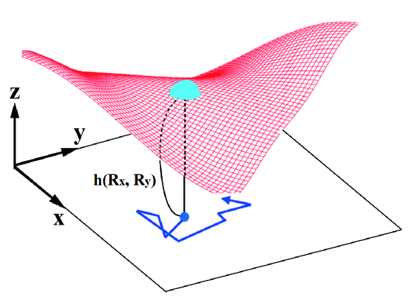
Figure 1: (Color online) The height variable $h(x,y)$ for a random surface indicated by the red mesh. The position of the Brownian particle (drawn in light blue) is given by $\vec{R}=(R_{x},R_{y},R_{z})$ with $R_{z}=h(R_{x},R_{y})$.

The quenched case where the shape relaxation is slow compared with the motion of a Brownian particle has been investigated less intensively. In one dimension, it has been shown that diffusion on a static surface is equivalent with Brownian motion in potential fields Zwanzig ; Halle . The formula for the diffusion constant has been derived for both periodic Lifson ; Jackson ; Festa and random potentials Zwanzig ; Halle . However, to the authors’ knowledge, no exact theory for the diffusion coefficient has been available so far for two-dimensional surfaces. We address this problem in the present study.

The quenched situation is expected in soft matter in thermal equilibrium, where interconnected structures with complex curved surfaces are often observed. Diffusion on such structures is highly non-trivial and the surface dynamics is not always relevant. Typical examples are organelles in living cells Sbalzarini and the sponge phase in microemulsions Gelbart . Actually simulations of diffusion on static curved biological surfaces have been conducted Sbalzarini .

One may also expect the quenched situation in non-equilibrium systems. For example, the migrating velocity of an active Brownian particle which undergoes self-propulsion consuming energy produced inside or on the surface of the particle Ebeling ; Ganguly can be larger than the velocity caused only by thermal fluctuations. Quite recently, such studies in confined geometries have been carried out both experimentally Wang and theoretically Castro . When a membrane is subjected to non-thermal noise out of equilibrium Ramaswamy , it might also increase the migration velocity.

The application of the present theory is not limited to the systems mentioned above. It is possible, for example, that the result is useful for understanding chemical kinetics of adatoms on rough solid surfaces Masel .

Langevin equation.—We consider a Brownian particle migrating on a surface in a simple model system as schematically shown in Fig. 1. The thickness of the surface is regarded as infinitesimal by assuming that the particle radius is much larger. Let us suppose that the particle is located at $\vec{R}(t)=(R_{x}(t),R_{y}(t),R_{z}(t))$ with $R_{z}=h(\vec{R}^{\perp}(t),t)$ and $\vec{R}^{\perp}=(R_{x},R_{y})$ where $h(\vec{r},t)$ is the height of the surface at $\vec{r}$ on the base plane. Naji and Brown have formulated a theory for Brownian motion on a fluctuating surface to derive the stochastic equation for the particle Naji1 . The random force acting on the particle is defined on the tangent plane at each point on the surface. They solved numerically the Langevin equation coupled with the time-evolution equation for the height variable to investigate the crossover from the annealed to quenched cases.

The stochastic equation of motion for a Brownian particle in the Naji-Brown theory Naji1 takes the form

$$\partial_{t}\vec{R}^{\perp}=Z\vec{\nu},$$ (1)

where $Z$ is a $2\times 2$ matrix whose components are given by

$$Z_{ij}=\delta_{ij}-\frac{(\partial_{i}h)(\partial_{j}h)}{g+\sqrt{g}}$$ (2)

with

$$g=1+(\partial_{x}h)^{2}+(\partial_{y}h)^{2}.$$ (3)

The argument $\vec{r}$ in the height variable should be replaced by $\vec{R}^{\perp}$ after taking spatial derivative. The random force $\vec{\nu}$ in Eq. (1) obeys Gaussian statistics with zero mean and

$$\langle\nu_{i}(t)\nu_{j}(t^{\prime})\rangle=2D_{0}\delta_{ij}\delta(t-t^{\prime}).$$ (4)

The positive constant $D_{0}$ is the diffusion coefficient on a flat plane. Since $Z$ depends on $\vec{\nu}$ through $h(\vec{R}^{\perp})$, the noise term in Eq. (1) is generally multiplicative. We employ the Stratonovich interpretation of the multiplicative noise, while Naji and Brown take the Ito prescription with an additive drift term in Eq. (1). This difference is not essential for deriving the diffusion coefficient. Naji and Brown have shown that Naji1

$$Z_{ik}Z_{jk}=(g^{-1})_{ij},$$ (5)

where the repeated indices imply summation. The tensor $g^{-1}$ is the inverse of the metric tensor $g_{ij}=\delta_{ij}+(\partial_{i}h)(\partial_{j}h)$ and is given by

$$(g^{-1})_{ij}=\delta_{ij}-\frac{(\partial_{i}h)(\partial_{j}h)}{g}.$$ (6)

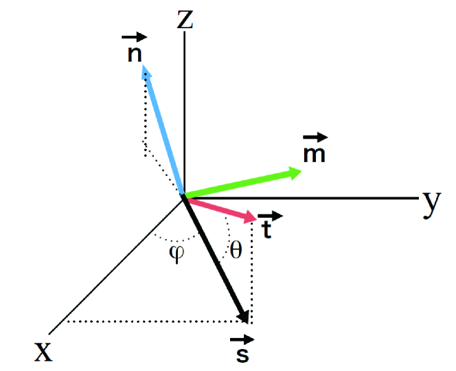
Figure 2: (Color online) The blue vector $\vec{n}$ is the normal unit vector, the red vector $\vec{t}$ the tangent unit vector, and the green vector $\vec{m}$ the unit vector perpendicular to both $\vec{n}$ and $\vec{t}$. The vector $\vec{s}$ ($|\vec{s}|\neq 1$) is a projection of $\vec{t}$ to the $x$-$y$ plane. The vector $\vec{m}$ is on the $x$-$y$ plane. The tangent plane touches the curved surface at $x=y=z=0$.

Here we describe an alternative derivation of the tensor $Z$, which has an intuitive implication. Let us introduce the tangent unit vector $\vec{t}$, normal unit vector $\vec{n}$, and vector $\vec{m}$ which is orthogonal to the former two vectors as depicted in Fig. 2. These unit vectors are defined, respectively, as

$$\vec{t} =\frac{1}{\sqrt{g}\sqrt{g-1}}(\partial_{x}h,\partial_{y}h,g-1)$$

$$=(\cos\theta\cos\phi,\cos\theta\sin\phi,\sin\theta),$$ (7)

$$\vec{n} =\frac{1}{\sqrt{g}}(-\partial_{x}h,-\partial_{y}h,1)$$

$$=(-\sin\theta\cos\phi,-\sin\theta\sin\phi,\cos\theta),$$ (8)

$$\vec{m} =-\frac{\vec{t}\times\vec{n}}{|\vec{t}\times\vec{n}|}=\frac{1}{\sqrt{g-1}}(-\partial_{y}h,\partial_{x}h,0)$$

$$=(-\sin\phi,\cos\phi,0),$$ (9)

where $\theta$ is the angle between $\vec{t}$ and the $x$-$y$ plane and $\phi$ the angle between the projected vector $\vec{s}=(\partial_{x}h,\partial_{y}h,0)/(\sqrt{g}\sqrt{g-1})$ and the $x$-axis as shown in Fig. 2 (notice that $|\vec{s}|\neq 1$). The unit vectors $\vec{t}$, $\vec{m}$ and $\vec{n}$ constitute a set of orthogonal coordinates at each point on the curved surface.

The velocity of the Brownian particle on the left hand side of Eq. (1) is defined on the base plane, whereas the random force on the right hand side is parallel to the tangent plane Naji1 . Keeping this fact in mind, we consider a mapping from the tangent to base planes. Let us introduce a vector on the tangent plane $\xi_{t}\vec{t}+\xi_{m}\vec{m}$ with arbitrary constants $\xi_{t}$ and $\xi_{m}$. The projection of this vector on the $x$-$y$ plane can be written as

$$\eta_{i}=\xi_{t}t_{i}+\xi_{m}m_{i}=Q_{ij}\xi_{j},$$ (10)

where the third component is excluded, i.e., $i,j=1,2$ and $\xi_{1}=\xi_{t}$ and $\xi_{2}=\xi_{m}$. From Eqs. (7) and (9), we find that the matrix $Q$ takes the form

$$Q=\left(\begin{array}[]{ccc}\dfrac{\partial_{x}h}{\sqrt{g}\sqrt{g-1}}&\dfrac{-\partial_{y}h}{\sqrt{g-1}}\\ \dfrac{\partial_{y}h}{\sqrt{g}\sqrt{g-1}}&\dfrac{\partial_{x}h}{\sqrt{g-1}}\end{array}\right).$$ (13)

However this is inadequate to enter directly in the Langevin equation (1) since the off-diagonal elements of $Q$ are not symmetric under the interchange $x\leftrightarrow y$, which is required by the isotropy of the base plane. We note that

$$P=QA$$ (14)

with

$$A=\frac{1}{\sqrt{g-1}}\left(\begin{array}[]{ccc}\partial_{x}h&\partial_{y}h\\ -\partial_{y}h&\partial_{x}h\end{array}\right)=\left(\begin{array}[]{ccc}\cos\phi&\sin\phi\\ -\sin\phi&\cos\phi\end{array}\right)$$ (19)

is the only choice in terms of the angle $\phi$ to satisfy the symmetry requirement. In fact, it is readily proved from Eqs. (13) and (19) that $P$ is equal to $Z$ given by Eq. (2). The relation in Eq. (5) is also verified by noting that

$$Q_{ik}Q_{jk}=(g^{-1})_{ij}$$ (20)

and $A_{ji}=(A^{-1})_{ij}$. The mapping in Eq. (10) is then written as

$$\vec{\eta}=P\vec{\zeta}$$ (21)

with $\vec{\zeta}=A^{-1}\vec{\xi}$.

Mean square displacement and lateral diffusion coefficient.—Now we solve Eq. (1) in the case of a random time-independent surface. The solution can be written formally as

$$R_{i}^{\perp}(t)-R_{i}^{\perp}(0) =\int d\vec{r}\,Z(h(\vec{r}))_{ij}$$

$$\times\int_{0}^{t}ds\,\delta(\vec{r}-\vec{R}^{\perp}(s))\nu_{j}(s),$$ (22)

from which one obtains

$$(\vec{R}^{\perp}(t)-\vec{R}^{\perp}(0))^{2} =\int d\vec{r}_{1}\int d\vec{r}_{2}\,Z(h(\vec{r}_{1}))_{ij}Z(h(\vec{r}_{2}))_{ik}$$

$$\times\int_{0}^{t}ds_{1}\int_{0}^{t}ds_{2}\,\delta(\vec{r}_{1}-\vec{R}^{\perp}(s_{1}))\nu_{j}(s_{1})$$

$$\times\delta(\vec{r}_{2}-\vec{R}^{\perp}(s_{2}))\nu_{k}(s_{2}).$$ (23)

The mean square displacement on the base plane can be obtained by averaging Eq. (23) over the randomness of the surface height and the random force. Since these are generally independent of each other for a frozen surface, one may write Eq. (23) as

$$\langle(\vec{R}^{\perp}(t)-\vec{R}^{\perp}(0))^{2}\rangle$$

$$=\int d\vec{r}_{1}\int d\vec{r}_{2}\,\langle Z(h(\vec{r}_{1}))_{ij}Z(h(\vec{r}_{2}))_{ik}\rangle_{h}$$

$$\times\int_{0}^{t}ds_{1}\int_{0}^{t}ds_{2}\,\langle\delta(\vec{r}_{1}-\vec{R}^{\perp}(s_{1}))\delta(\vec{r}_{2}-\vec{R}^{\perp}(s_{2}))$$

$$\times\nu_{j}(s_{1})\nu_{k}(s_{2})\rangle_{\vec{\nu}},$$ (24)

where $\langle\cdots\rangle_{h}$ and $\langle\cdots\rangle_{\vec{\nu}}$ indicate the average over $h$ and $\vec{\nu}$, respectively. Since we have assumed that the randomness of the height does not have any spatial correlation, the decoupling $\langle Z(h(\vec{r}_{1}))_{ij}Z(h(\vec{r}_{2}))_{ik}\rangle_{h}=\langle Z(h(\vec{r}_{1}))_{ij}\rangle_{h}\langle Z(h(\vec{r}_{2}))_{ik}\rangle_{h}$ is allowed and each part is constant in space because of the translational invariance. Therefore, one has

$$\langle(\vec{R}^{\perp}(t)-\vec{R}^{\perp}(0))^{2}\rangle=\langle Z_{ij}\rangle_{h}\langle Z_{ij}\rangle_{h}2D_{0}t=2dDt,$$ (25)

where $d$ is the dimensionality of the surface and we have used Eq. (4). The effective diffusion coefficient $D$ will be obtained shortly. The expression in Eq. (25) implies that taking an average of $Z$ in the Langevin equation (1) with respect to the surface randomness is justified. By using the isotropy of space, the effective lateral diffusion coefficient $D$ is given for $d=2$ by

$$\frac{D}{D_{0}}=\langle Z_{11}\rangle^{2}_{h}=\left\langle\frac{1}{2}\left(1+\frac{1}{\sqrt{g}}\right)\right\rangle_{h}^{2}.$$ (26)

This is the main result of this Letter. When the surface is a curved line embedded in two dimensions, on the other hand, only the element $Z_{11}=1/\sqrt{g}$ exists and one obtains for $d=1$

$$\frac{D}{D_{0}}=\left\langle\frac{1}{\sqrt{g}}\right\rangle_{h}^{2}.$$ (27)

This is the known exact result Halle ; Naji1 and has also been obtained by the present method Ohta ; comment .

The ensemble average can be replaced by the surface average (the contour average in one dimension) defined as Gustafsson

$$\langle A\rangle_{s}\equiv\frac{\int_{0}^{L}\int_{0}^{L}dx\,dy\,\sqrt{g}A}{\int_{0}^{L}\int_{0}^{L}dx\,dy\,\sqrt{g}},$$ (28)

where $L$ is the system size. Hereafter we shall use this notation of the average $\langle\cdots\rangle_{s}$.

Figure 3: The scaled diffusion coefficient $D/D_{0}$ (solid line), the upper and lower bounds $D_{U}/D_{0}$ (dotted line), and $D_{L}/D_{0}$ (dashed line) given by Eqs. (35), (36), and (37), respectively, as a function of $w=\langle(\vec{\nabla}h)^{2}\rangle^{1/2}$ for a quenched Gaussian random surface.

The upper and lower bounds for the diffusion coefficient in two dimensions have been obtained, respectively, as Gustafsson

$$\frac{D_{U}}{D_{0}}=\frac{1}{2}\left(1+\left\langle\frac{1}{g}\right\rangle_{s}\right),$$ (29)

$$\frac{D_{L}}{D_{0}}=\frac{2\left\langle 1/\sqrt{g}\right\rangle_{s}^{2}}{1+\left\langle 1/g\right\rangle_{s}}.$$ (30)

In order to prove $D_{L}\leq D\leq D_{U}$, the inequality

$$\langle A\rangle^{2}\leq\langle A^{2}\rangle$$ (31)

is useful. Applying this to Eq. (26), one has

$$\frac{D}{D_{0}} =\left(\left\langle\frac{1}{2}\left(1+\frac{1}{\sqrt{g}}\right)\right\rangle_{s}\right)^{2}$$

$$\leq\left\langle\left(\frac{1}{2}\left(1+\frac{1}{\sqrt{g}}\right)\right)^{2}\right\rangle_{s}.$$ (32)

It is readily shown that the last expression in Eq. (32) is smaller than $D_{U}$ so that $D\leq D_{U}$.

On the other hand, the lower bound Eq. (30) satisfies

$$\frac{D_{L}}{D_{0}}=\frac{2\left\langle 1/\sqrt{g}\right\rangle_{s}^{2}}{1+\left\langle 1/g\right\rangle_{s}}\leq\frac{2\left\langle 1/\sqrt{g}\right\rangle_{s}^{2}}{1+\left\langle 1/\sqrt{g}\right\rangle^{2}_{s}}.$$ (33)

It is easy to see that $D$ is larger than the last expression of Eq. (33) leading to $D_{L}\leq D$.

In the above, we have presented a mathematically rigorous proof for $D_{L}\leq D\leq D_{U}$. It might be useful, however, to show the relative magnitude and all over behavior of these three quantities. This is possible if the probability distribution of $\vec{p}=\vec{\nabla}h$ is Gaussian Gustafsson

$$f(p)=\frac{2}{w^{2}}\exp\Big{(}-\frac{\vec{p}^{2}}{w^{2}}\Big{)},$$ (34)

where $w=\langle(\vec{\nabla}h)^{2}\rangle^{1/2}$ is the root-mean-square fluctuation. The function $f(p)$ is normalized as $\int_{0}^{\infty}dp\,pf(p)=1$. The exact diffusion coefficient $D$ in Eq. (26) turns out to be

$$\frac{D}{D_{0}}=\frac{1}{4}[1+\sqrt{\pi}(1/w)\exp(1/w^{2})\,{\rm erfc}(1/w)]^{2},$$ (35)

where ${\rm erfc}(x)=(2/\pi)\int_{x}^{\infty}dt\,e^{-t^{2}}$. On the other hand, the explicit forms of the upper and lower bounds given by Eqs. (29) and (30), respectively, have been obtained for Gaussian surfaces as Gustafsson

$$\frac{D_{U}}{D_{0}}=\frac{1}{2}\left[1+(1/w^{2})\exp(1/w^{2})E_{1}(1/w^{2})\right],$$ (36)

$$\frac{D_{L}}{D_{0}}=\frac{2\pi[(1/w)\exp(1/w^{2})\,{\rm erfc}(1/w)]^{2}}{1+(1/w^{2})\exp(1/w^{2})E_{1}(1/w^{2})},$$ (37)

where $E_{1}(x)=\int_{x}^{\infty}dt\,e^{-t}/t$. In Fig. 3, Eqs. (35), (36), and (37) are plotted as a function of $w$. The diffusion coefficient $D/D_{0}$ decreases monotonically as $w$ is increased, approaching to the asymptotic value of 1/4.

Discussion.—Gustafsson and Halle Gustafsson have argued that there are two candidates for the diffusion coefficient on the frozen disordered surface. Although our result in Eq. (26) is exact, we compare it with other formulas. One is the result obtained by the area scaling in analogy with the projected contour length in one dimension Halle ; Gustafsson

$$\frac{D_{A}}{D_{0}}=\left\langle\frac{1}{\sqrt{g}}\right\rangle_{s}.$$ (38)

The other is obtained by the effective medium approximation Gustafsson

$$\frac{D_{M}}{D_{0}}=\frac{1}{\langle\sqrt{g}\rangle}_{s}.$$ (39)

The requirement $D_{L}\leq D_{A},D_{M}\leq D_{U}$ has been verified for small values of $(\vec{\nabla}h)^{2}$ Gustafsson .

One of the most distinct differences between the present result in Eq. (26) and the approximants in Eqs. (38) and (39) is that $D$ is finite for $g\rightarrow\infty$, whereas both $D_{A}$ and $D_{M}$ vanish in this limit. Even if local maxima (minima) in a two-dimensional surface are extremely high (deep), Brownian motion parallel to the base plane is always possible without being totally blocked so that it produces finite displacement. In fact, the elements of the matrix $Z$ for $\theta=\pi/2$ are given by $Z_{11}=\sin^{2}\phi$, $Z_{12}=Z_{21}=-\sin\phi\cos\phi$ and $Z_{22}=\cos^{2}\phi$. The average over the angle $\phi$ yields $\langle Z_{11}\rangle_{\phi}\equiv(1/2\pi)\int_{0}^{2\pi}d\phi\,Z_{11}=1/2$, whose square gives rises to the factor $1/4$ in the diffusion coefficient $D$ in Eq. (26). In contradiction to this, the diffusion coefficient obtained by numerical simulations of the Langevin equation seems consistent with $D_{A}$ even for large values of the surface roughness $w$ as shown in Figs. 9 and 10 in Ref. Naji1 . The reason for this is unclear at present. It is geometrically obvious that the above argument does not hold in one dimension. Actually the diffusion constant in Eq. (27) vanishes in the limit $g\rightarrow\infty$

Summary.—In summary, the present theory provides an exact prediction for the diffusion coefficient on a two-dimensional frozen surface, which satisfies the restriction due to the upper and lower bounds. We start with the Langevin equation for a Brownian particle on a random surface formulated by Naji and Brown Naji1 . The lateral diffusion coefficient is obtained by averaging the coefficient multiplied by the random force, which is valid in the quenched limit for random surfaces without any spatial correlation.

T.O. is indebted to Dr. Kazuhiko Seki for bringing his attention to Ref. Zwanzig . S.K. thanks Yuto Hosaka for useful discussion. S.K. acknowledges support by a Grant-in-Aid for Scientific Research (C) (Grant No. 18K03567 and Grant No. 19K03765) from the Japan Society for the Promotion of Science and support by a Grant-in-Aid for Scientific Research on Innovative Areas “Information Physics of Living Matters” (Grant No. 20H05538) from the Ministry of Education, Culture, Sports, Science and Technology of Japan.

References

- (1) Marguet D. and Salome L., in Physics of Biological Membranes, edited by P. Bassereau and P. Sens (Springer Nature, Switzerland, 2018), pp. 169-189.
- (2) Axelrod D., Koppel D. E., Schlessinger J., Elson E. and Webb W. W., Biophys. J. 16, (1976) 1055.
- (3) Sprague B. L., Pego R. L., Stavreva D. A. and McNally J. G., Biophys. J. 86, (2004) 3473.
- (4) Lee G., Ishihara A. and Jacobson K. A., Proc. Natl. Acad. Sci. USA, 88, (1991) 6274.
- (5) Kusumi A., Nakada C., Ritchie K., Murase K., Suzuki K., Murakoshi H., Kasai R. S., Kondo J. and Fujiwara T., Annu. Rev. Biophys. Biomol. Struct. 34, (2005) 351.
- (6) Safmann P. G. and Delbrück M., Proc. Natl. Acad. Sci. USA 72, (1975) 3111.
- (7) Block S., Biomolecules 8, (2018) 30.
- (8) Aizenbud B. M. and Gershon N. D., Biophys. J. 38, (1982) 287.
- (9) Halle B. and Gustafsson S., Phys. Rev. E 55, (1997) 680.
- (10) Gustafsson S. and Halle B., J. Chem. Phys. 106, (1997) 1880.
- (11) Naji A. and Brown F. L. H., J. Chem. Phys. 126, (2007) 235103.
- (12) Naji A., Atzberger P. J. and Brown F. L. H., Phys. Rev. Lett. 102, (2009) 138102.
- (13) Reister-Gottfried E., Leitenberger S. M. and Seifert U., Phys. Rev. E 81, (2010) 031903.
- (14) Ohta T., J. Phys. Soc. Jpn. 89, (2020) 074001.
- (15) Zwanzig R., Proc. Natl. Acad. Sci. USA 85, (1988) 2029.
- (16) Lifson S. and Jackson J. L., J. Chem. Phys. 36, (1962) 2410.
- (17) Jackson J. L. and Coriell S. M., J. Chem. Phys. 38, 959 (1963).
- (18) Festa R. and d’Agliano E. Galleani, Physica A 90, (1978) 229.
- (19) Sbalzarini I. F., Hayer A., Helenius A. and Koumoutsako P., Biophys. J. 90, (2006) 878.
- (20) Gelbart W. M., Ben-Shaul A. and Roux D. (Eds.), Micelles, Membranes, Microemulsions and Monolayers (Springer, New York, 1994).
- (21) Ebeling W., Acta Physica Polonica B, 38, (2007) 1657.
- (22) Ganguly C. and Chaudhuri D., Phys. Rev. E 88, (2013) 032102.
- (23) Wang X., In M., Blanc C., Nobili M. and Stocco A., Soft Matter 11, (2015) 7376.
- (24) Castro-Villarreal P. and Sevilla F. J., Phys. Rev. E 97, (2018) 052605.
- (25) Ramaswamy S., Toner J. and Prost J., Phys. Rev. Lett. 84, (2000) 3494.
- (26) Masel R. I., Principles of Adsorption and Reaction on Solid Surfaces (John Wiley Sons, New York, 1996).
- (27) The spatial average in Eq. (A.13) in Ref. Ohta should read the surface (contour) average.