Global analysis of more than 50,000 SARS-Cov-2 genomes reveals epistasis between 8 viral genes

Abstract

Genome-wide epistasis analysis is a powerful tool to infer gene interactions, which can guide drug and vaccine development and lead to deeper understanding of microbial pathogenesis. We have considered all complete SARS-CoV-2 genomes deposited in the GISAID repository until four different cut-off dates, and used Direct Coupling Analysis together with an assumption of Quasi-Linkage Equilibrium to infer epistatic contributions to fitness from polymorphic loci. We find eight interactions, of which three between pairs where one locus lies in gene ORF3a, both loci holding non-synonymous mutations. We also find interactions between two loci in gene nsp13, both holding non-synonymous mutations, and four interactions involving one locus holding a synonymous mutation. Altogether we infer interactions between loci in viral genes ORF3a and nsp2, nsp12 and nsp6, between ORF8 and nsp4, and between loci in genes nsp2, nsp13 and nsp14. The paper opens the prospect to use prominent epistatically linked pairs as a starting point to search for combinatorial weaknesses of recombinant viral pathogens.

I Introduction

The pandemic of the disease COVID-19 has so far led to the confirmed deaths of more than 991,224 people World Health Organization (2020) and has hurt millions. As the health crisis has been met by Non-Pharmacological Interventions Moritz et al. (2020); Salje et al. (2020) there has been significant economic disruption in many countries. The search for vaccine or treatment against the new coronavirus SARS-CoV-2 is therefore a world-wide priority. The GISAID repository Shu and McCauley (2017) contains a rapidly increasing collection of SARS-CoV-2 whole-genome sequences, and has already been leveraged to identify mutational hotspots and potential drug targets Pachetti et al. (2020). Coronaviruses in general exhibit a large amount of recombination Lai and Cavanagh (1997); Graham and Baric (2010); Gribble et al. (2020); Li et al. (2020a). The distribution of genotypes in a viral population can therefore be expected to be in the state of Quasi-Linkage Equilibrium Kimura (1965); Neher and Shraiman (2009, 2011), and directly related to epistatic contributions to fitness Gao et al. (2019); Zeng and Aurell (2020). We have determined a list of the largest such contributions from 51,676 SARS-CoV-2 genomes by a Direct Coupling Analysis (DCA) Morcos et al. (2011); Cocco et al. (2018). This family of techniques has earlier been used to infer the fitness landscape of HIV-1 Gag Shekhar et al. (2013); Mann et al. (2014) to connect bacterial genotypes and phenotypes through co-evolutionary landscapes Cheng et al. (2016) and to enhance models of amino acid sequence evolution de la Paz et al. (2020). We apply a recent enhancement of this technique to eliminate predictions that can be attributed to phylogenetics (shared inheritance) Horta et al. (2019). We find that eight predictions stand out between pairs of polymorphic sites located in genes nsp2 and ORF3a, nsp4 and ORF8, and between genes nsp2, nsp6, nsp12, nsp13, nsp14 and ORF3a. Most of these sites have been documented in the literature when it comes to single-locus variations Forster et al. (2020); Khailany et al. (2020); Cai et al. (2020); Deng et al. (2020); Phelan et al. (2020); Sashittal et al. (2020). The nsp4-ORF8 pair was additionally found to be strongly correlated in an early study Tang et al. (2020). It does not show prominent correlations today, but is ranked second in our global analysis. The epistasis analysis of this paper brings a different perspective than correlations, and highlights pairwise associations that have remained stable as orders of more SARS-CoV-2 genomes have been sequenced.

II Data and Methods

II.1 Genome Data of SARS-CoV-2

We analyzed the consensus sequences deposited in the GISAID database Shu and McCauley (2017) with high quality and full lengths (number of bps $\approx 30,000$). Four data-sets are used for our investigation according to the collection date in GISAID database. The dates are 2020-04-01, 2020-04-08, 2020-05-02 and 2020-08-08 respectively. The list of GISAID sequences used is available on the Github repository Zeng (2020). The numbers of selected genomes are 2,268, 3,490, 10,587 and 51,676 for each collection date.

II.2 Multiple-Sequence Alignment (MSA)

Multiple sequence alignments were constructed with the online alignment server MAFFT Katoh et al. (2017); Kuraku et al. (2013) for the two smaller data sets with cut-off dates 2020-04-01 and 2020-04-08. To align the two larger data-set with more than 10,000 sequences, a pre-aligned reference MSA is recommended to accelerate the alignment and reduce the burden on computational resources. Here, we took the collection with cut-off date 2020-04-08 as the pre-aligned reference MSA for the two largest data set with cut-off dates 2020-05-02 and 2020-08-08. The MSAs used are available on the Github repository Zeng (2020).

The MSA is a big matrix $\mathbf{S}=\{\sigma_{i}^{n}|i=1,...,L,n=1,...,N\}$, composed of $N$ genomic sequences which are aligned over $L$ positions Cocco et al. (2018); Horta et al. (2019). Each entry $\sigma_{i}^{n}$ of matrix $\mathbf{S}$ is either one of the 4 nucleotides (A,C,G,T), or “not known nucleotide” (N), or the alignment gap ‘-’ introduced to treat nucleotide deletions or insertions, or some minorities.

II.3 MSA filtering

Before filtering, we transform the MSA in two different ways as follows:

• The gaps ‘-’ are transformed to ‘N’ while the minors ‘KFY…’ are mapped to ‘N’. There thus 5 states remains, where ‘NACGT’ are represented by ‘12345’;

• The minors ‘KFY…’ are mapped to ‘N’. Then there are 6 states, with ‘-NACGT’ represented by ‘012345’.

The following criteria are used for pre-filtering of the MSA from the 2020-08-08 data-set. If for one locus the same nucleotide is found in more than 96.5% of this column, or if the sum of the percentages of A, C, G and T at this position is less than 20%, then this locus will be deleted. For each sequence, if the percentage of a certain nucleotide is more than 80%, or if the sum of the percentages of A, C, G and T in this sequence is less than 20%, then this sequence will be deleted. With this filtering criteria, many loci but no sequences are deleted. There are left 51,676 sequences and 689 loci.

II.4 B-effective number

To mitigate the effects of dependent samplings, it is standard practice to attach to each collected genome sequence $\sigma^{(b)}$ a weight $w_{b}$ Morcos et al. (2011); Ekeberg et al. (2014); Cocco et al. (2018), which normalizes its impact on the inference procedure. An efficient way to measure the similarity between two sequences $\sigma^{(a)}$ and $\sigma^{(b)}$ is to compute the fraction of identical nucleotides and compare it with a preassigned threshold value $x$ in the range $0\leq x\leq 1$. The weight of a sequence $\sigma^{(b)}$ can be set as $w_{b}=\frac{1}{m_{b}}$, with $m_{b}$ the number of sequences in the MSA that are similar to $\bm{\sigma}^{(b)}$:

$$m_{b}=|\{a\in\{1,...,B\}\}\texttt{:overlap}(\bm{\sigma}^{(a)},\bm{\sigma}^{(b)})\geq x|;$$ (1)

here overlap is the fraction of loci where the two sequences are identical. The B-effective number of the transformed sequences is defined as

$$B_{eff}=\sum_{b=1}^{B}w_{b}.$$ (2)

We compare the $B_{eff}$ value with different $x$ for the filtered MSA with $q=5$ and $q=6$ respectively. As shown in Fig. 1, the data-set with 6 states shows larger $B_{eff}$ number for all tested $x$. We thus perform our analysis on the data-set with $q=6$ states, where ‘-NACGT’ represented by ‘012345’.

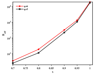
Figure 1: $B_{eff}$ number of the 2020-08-08 pre-filtered data-set with threshold $x$. Red for $q=6$ states (‘-NACGT’) and black for $q=5$ states (‘NACGT’). The number of states are determined by the transform criteria of the pre-filtered MSA.

The re-weighting procedure partially addresses a point raised  MacLean et al. (2020), that sequenced viral genomes are not a random sample of the global population. That is, even if sequencing is biased by the country they occur in and by contact tracing, sufficiently similar genomes will have lower weight and so each will contribute less to predictions.

II.5 Elements of Quasi-Linkage-Equilibrium (QLE)

The phenomenon of QLE was discovered by M. Kimura while investigating the steady-state distribution over two bi-allelic loci evolving under mutation, recombination and selection, with both additive and epistatic contributions to fitness Kimura (1965). In the absence of epistasis such a system evolves toward Linkage Equilibrium (LE) where the distribution of alleles at the two loci are independent. The covariance of alleles at the two loci then vanishes. In the presence of pairwise epistasis and sufficiently high rate of recombination, the steady-state distribution takes form of a Gibbs-Boltzmann form

$$P(\sigma_{1},...,\sigma_{L})=\frac{1}{Z}\exp\{-H(\sigma_{1},...,\sigma_{L})\},$$ (3)

with an ”energy function”

$$H(\sigma_{1},...,\sigma_{L})=\sum_{i}h_{i}(\sigma_{i})+\sum_{ij}J_{ij}(\sigma_{i},\sigma_{j})$$ (4)

In above $J_{ij}$ can be related to the epistatic contribution to fitness between loci $i$ and $j$ with alleles $\sigma_{i}$ and $\sigma_{j}$ Neher and Shraiman (2009, 2011); Gao et al. (2019). The quantity $h_{i}$ is similarly a function of allele $\sigma_{i}$ which depends on both additive and epistatic contributions to fitness involving locus $i$. It has been verified in in silico testing that when the terms in (4) can be recovered this is a means to infer epistatic fitness from samples of genotypes in a population Zeng and Aurell (2020). In the bacterial realm this approach was used earlier to infer epistatic contributions to fitness in the human pathogens Streptococcus pneumonia Skwark et al. (2017) and Neisseria gonorrhoeae Schubert et al. (2019), both of which are characterized by a high rate of recombination. The method was also tested on data on the bacterial pathogen Vibrio parahemolyticus Cui et al. (2020). In that study the results from DCA were not superior from an analysis based on Fisher exact test, see Appendix G for a discussion. This is consistent with the approach taken here, as V. parahemolyticus has low rate of recombination. Further details on the QLE state of evolving populations are given in Appendix A.

II.6 Inference Method for epistasis between loci

The basic assumption of modeling the filtered MSA is that it is composed by independent samples that follows the Gibbs-Boltzmann distribution (3) with $H$ as in (4) Higher order interactions are also possible to include, but we ignore them here Schneidman et al. (2006). This assumption is a simplification of the biological reality, however provides an efficient way to extract information from massive data.

On the other hand, in the context of inference from protein sequences, it has been argued that the one encoded in Eq. (3-4) is the minimal generative model i.e. capable not only to reproduce the empirical frequencies and correlations but also to generate new sequences indistinguishable from natural sequences Cocco et al. (2018); Russ et al. (2005); Socolich et al. (2005).

Many techniques have been developed to infer the direct couplings in Eq. (3), as reviewed in Nguyen et al. (2017) and references therein, see also Appendix C. We employ the maximum pseudo-likelihood (PLM) method Besag (1975); Ravikumar et al. (2010); Aurell and Ekeberg (2012); Ekeberg et al. (2013, 2014); Gao et al. (2019) to infer the epistatic effects between loci from the aligned MSA. PLM estimates parameters from conditional probabilities of one sequence conditioned on all the others. For Potts model with multiple states $q>2$, this conditional probability is

$$P(\sigma_{i}|\bm{\sigma}_{\backslash i})=\frac{\exp\left(h_{i}(\sigma_{i})+\sum_{j\neq i}J_{ij}(\sigma_{i},\sigma_{j})\right)}{\sum_{\mathbf{u}}\exp\left(h_{i}(u)+\sum_{j\neq i}J_{ij}(u,\sigma_{j})\right)},$$ (5)

with $\mathbf{u}=\{0,1,2,3,4,5\}$ the possible state of $\sigma_{i}$. Eq. (5) depends on a much smaller parameter set compared with that in Eq. (3). This leads a much faster inference procedure of parameters compared with the maximum likelihood method. With a given independent sample sets, one can maximize the corresponding log-likelihood function

$$PL_{i}\left(h_{i},\{J_{ij}\}\right)=\frac{1}{N}\sum_{s}h_{i}\left(\sigma_{i}^{(s)}\right)+\frac{1}{N}\sum_{s}\sum_{j\neq i}J_{ij}(\sigma_{i}^{(s)},\sigma_{j}^{(s)})-\frac{1}{N}\sum_{s}\log\sum_{\mathbf{u}}\exp\big{(}h_{i}(u)+\sum_{j\neq i}J_{ij}(u,\sigma_{j}^{(s)})\big{)},$$ (6)

where $s$ labels the sequences (samples), from $1$ to $N$. With the filtered MSA, we then run the asymmetric version of PLM Ekeberg et al. (2014) in the implementation PLM available on Gao (2018) with regularization parameter $\lambda=0.1$. The inferred interactions between loci $i$ and $j$ are scored by the Frobenius norm.

II.7 Relation to correlation analysis

In LE the distributions of alleles over different loci are independent. Given unlimited data and unlimited computational resources, the terms $J_{ij}$ in (4) inferred from the data would then be zero. The locus-locus co-variances, defined as

$$c_{ij}(a,b)=\left<\mathbf{1}_{\sigma_{i},a}\mathbf{1}_{\sigma_{j},b}\right>-\left<\mathbf{1}_{\sigma_{i},a}\right>\left<\mathbf{1}_{\sigma_{j},b}\right>$$ (7)

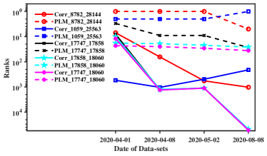
Figure 5: Ranks for significant epistatic effects with data collection date (2020-04-01, 2020-04-08, 2020-05-02 and 2020-08-08) by PLM (dashed lines) and correlation analysis (solid lines). The ranks of the PLM scores are almost constant while the ranks of the correlations vary significantly and mostly drop as more data accumulate (later cut-off dates).

would also be zero. The Frobenius norm of $c_{ij}(a,b)$ over indices $(a,b)$ as a score of strength of correlations would be zero as well. The qualitative difference between correlation analysis and global model inference based on (3) and (4) is that two loci $i$ and $j$ may be correlated (”indirectly coupled”) even if their interaction $J_{ij}$ is zero, provided they both interact with a third locus $k$. Data in Table 4 and Fig. 5 show that the leading interactions retrieved by DCA cannot be stably recovered in correlation analysis. A different score of statistical dependency between two categorical random variables is mutual information (MI). Appendix G shows that the result does not substantially change if using MI instead of Frobenuis norm of correlation matrices. Circos plots of interactions based on correlation scores are available on Zeng (2020).

II.8 Epistasis analysis with PLM scores

PLM procedure yields a fully connected paradigm between pairwise loci. To extract important information form massive SARS-CoV-2 genomic sequences, we focus on the significant scores between loci, the top-200 pairs. With a reference sequence “Wuhan-Hu-1”, we identify the positions of the corresponding nucleotides. The visualization of these epistasis is performed by ‘circos’ software Krzywinski et al. (2009).

II.9 Randomized background distributions

A way to assess the validity of a small number of leading retained predictions among a much larger set of mostly discarded predictions is to compare to randomized backgrounds. The retained predictions are then in any case large (by some measure) and would also be retained if selection would be made according to some cut-off, or an empirical $p$-value. The problem is thus how to distinguish the case where a small sub-set of retained values are large because they are different, from the case when in a large number of samples such values would appear at random. This problem can be addressed by comparing the retained values to the largest values from the same procedure applied to randomized data, as was done for predicted RNA-RNA binding energies in a non-coding RNA discovery pipeline Mandin et al. (2007). In the context of DCA (PLM) applied to genome-scale MSAs, two earlier studies relying on randomized background distributions are Xu et al. (2018) and Gao et al. (2019).

II.10 PLM scores with randomization

To understand the nature of the top-200 PLM scores we perform two distinct randomization strategies on the MSA, such that its conservation patterns and (or) phylogenetic relations are preserved, while intrinsic co-evolutionary couplings (epistatic interactions) are removed Horta and Weigt (2020). Running DCA on artificial sequences ensembles generated by these strategies, and comparing them to the results obtained from original MSA allows to disentangle spurious couplings given by finite-size effects or by phylogeny. The first strategy, we refer as ’profile’, randomizes the input MSA by random but independent permutation of all its columns conserving the single-columns statistics for all sites. This destroys all kind of correlations and DCA couplings inferred from such samples are only non-zero due to the noise caused by finite sample-size. In the second strategy referred as ’phylogeny’, the original MSA is randomized by a simulated annealing schedule where columns and rows are changed simultaneously but so that inter-sequence distances are kept invariant. Phylogeny inferred from inter-sequence distance information would therefore be unchanged. Conversely, if the predicted epistatic interactions are due to phylogeny, they should also show up in terms recovered by PLM from MSAs scrambled by ’phylogeny’. More details on the randomization strategies can be found in Appendix D.

III Results

The predicted effective interactions between loci were obtained from Pseudo-Likelihood Maximization (PLM) scores, a standard computational method to perform DCA. Manual inspection shows that about half of the top-50 links and most of the top-200 involve noncoding sites in the 5’ or 3’ region on the “Wuhan-Hu-1” Wu et al. (2020) reference sequence, many of them have very short range and most of them with a large fraction of the gap or N (unknown nucleotide) symbols (data available on Zeng (2020) for other data-set). We present the links with both terminal loci located in coding regions and the mutations excluding gaps or ‘N’s.

In Table 1 we list the significant links for the 2020-08-08 data-set. The first column is the index of each pairwise interaction in the top 200s. The second column indicates the locus with lower genomic position in the pair and the name of the SARS-CoV-2 proteins it belongs to. The third column lists the major / minor allele (most prevalent, second most prevalent nucleotide) and the mutation type at that locus. The following two columns provide similar information on the locus with higher genomic position in the pair. The last column contains the PLM scores indicating the strength of effects between pairs of loci. The pairwise epistasis listed in Table 1 for 2020-08-08 dataset are visualized by circos software in Fig. 2, where the red ones for the close effects (the distance between two loci is less or equal to 3 locus) while blue for distant effects. Analogous results for the 2020-05-02 dataset is shown in Appendix L, and for the 2020-04-01 and 2020-04-08 data-sets on Zeng (2020).

To check if the interactions can be explained by phylogeny (inherited variations) we used two randomization strategies ‘profile’ and ‘phylogeny’ of the Multiple Sequence Alignments (MSAs). Profile preserves the distribution over alleles at every locus but does so independently at each locus. Profile hence destroys all systematic co-variations between loci. Phylogeny additionally preserves the genetic distance between each pair of sequences. Viral genealogies inferred from this information are therefore unchanged under this randomization. PLM scores run on these two types of randomized data (scrambled MSAs) is a background from which the significance of the interactions from the original data can be assessed. Each randomization strategy is repeated 50 times with different realizations of the scrambling, see Appendix E and Zeng (2020). As shown in Fig. 3 the distribution of PLM scores using phylogeny and profile are qualitatively different from PLM scores of the original MSA, with progressively fewer interactions at high score values. With profile randomization, no interactions predicted by PLM appear with scores standing out from the background. Phylogeny randomization on the other hand preserves some interactions found by PLM in a fraction of the realizations of the random background. Table 2 lists interactions predicted by PLM that appear in some phylogeny randomizations with scores large compared to the background. In the following analysis we have not retained them, see Appendix E for circos visualizations. Table 3 lists the eight interactions found by PLM which either do not appear in any phylogeny randomization with scores that stand out from the background, or, in the case of (1059-25563), shows up three times in top-200 out of 50 samples. We retain these eight predicted epistatic interactions in the sampled populations of SARS-CoV-2 genomes. The top ones listed in Table 3 are marked by red arrows in Fig. 3(a).

Epistatic interactions obtained from DCA reflect pairwise statistical associations, but not correlations. As reviewed in Nguyen et al. (2017), and described in Appendix C, DCA is based on a global probabilistic model, and therefore ranks inter-dependency differently than correlations. Fig. 4 compared to Fig. 3 shows that the distribution of correlation scores is qualitatively different from the distributions of DCA scores in the GISAID data set. Fig. 5 further shows that the rank of the epistatic interaction predicted in Table 3 have remained stable, while the corresponding correlations have merged into the background.

The first-ranked interaction between 1059 and 25563 is between a (C/T), resulting in the T85I non-synonymous mutation in gene nsp2 and a (G/T), resulting in the Q57H non-synonymous mutation in gene ORF3a. nsp2, expressed as part of the ORF1a polyprotein, binds to host proteins prohibitin 1 and prohibitin 2 (PHB1 and PHB2) in SARS-CoV Yoshimoto (2020). The variations in the site 1059 have been predicted to modify nsp2 RNA secondary structure Hosseini and Donald (2020) and have previously been reported to co-occur together with the Q57H variant in ORF3a in a dataset of SARS-CoV-2 genomes from the United States  Rui et al. (2020). ORF3a, also known as ExoN1 hypothetical protein sars3a, forms a cation channel of which the structure in SARS-CoV-2 is known by Cryo-EM Kern et al. (2020). In SARS-CoV ORF3a been shown to up-regulate expression of fibrinogen subunits FGA, FGB and FGG in host lung epithelial cells Tan et al. (2005), to form an ion channel which modulates virus release Lu et al. (2006), to activate the NLRP3 inflammasome Siu et al. (2019), and has been found to induce apoptosis Ren et al. (2020). The Q57H variant was reported early in the COVID-19 pandemic Elio et al. (2020) and occurs in the first transmembrane alpha helix, TM1 Kern et al. (2020), where it changes the amino acid glutamine (Q) with a non-charged polar side chain to histidine (H), which has a positively charged polar side chain. This amino acid is at the interface of interaction between the two dimeric subunits of ORF3a that forms the constrictions of the ion channel but the Q57H alteration does not seem to change the ion channel properties compared to wildtype 3a  Kern et al. (2020). Nevertheless, its incidence is increasing in SARS-CoV-2 genomes in the United States Rui et al. (2020) and the effect of Q57H may therefore affect the virulence in other beneficial ways than changing the conductance properties of the ion pore.

The association between 8782 and 28144 (rank 5), reported early in SARS-CoV-2 studies Tang et al. (2020) is between a (C/T) synonymous mutation in the gene nsp4, and a (T/C) non-synonymous mutation resulting in the L84S alteration in the gene ORF8. The first of these genes participates in the assembly of virally-induced cytoplasmic double-membrane vesicles necessary for viral replication. The site 8782 is located in a region annotated as CpG-rich and is the site of a CpG for the major allele (C); it has the minor (T) allele in other related viruses Tang et al. (2020). Orf8 has been implicated in regulating the immune response Zhang et al. (2020); Li et al. (2020b). The L84S variant is, together with the C8782T nsp4 mutation characterizing the GISAID clade S Daniele and M. (2020).

The interaction between 14805 and 26144 (rank 9) leads to non-synonymous alterations in nsp12 (T455I, note that the reference is Y) and ORF3a (G251V) respectively. The G251V has been reported by many studies and is defining the GISAID V clade  Daniele and M. (2020) together with the L37F nsp6 variant (position 11083, rank 47). The widely reported G251V variant is unfortunately outside of the proposed Cryo-EM structure  Kern et al. (2020) and it is unknown how this glycine to valine substitution affects protein function. nsp12 is the RNA-dependent RNA polymerase and the T455I substitution is found where the reference Wuhan-Hu-1 has a tyrosine residue in one of the alpha helices of the polymerase ”finger” domain Chen et al. (2020). Threonine can similarly to tyrosine be phosphorylated but also glycosylated, it is polar, uncharged and can form hydrogen bonds that may stabilize the alpha helix. Isoleucine on the other hand is non-polar and uncharged and both the residues are smaller than the aromatic tyrosine.

The second interaction partner of G251V is the nsp6 L37F variant. nsp6 has been shown to induce autophagosomes in the host cells in favour for viral replication and propagation SARS-CoV Yoshimoto (2020). There is currently no experimentally validated model of nsp6 structure but an early model suggest that the L37P variant is situated in an unordered loop between two alpha helices Benvenuto et al. (2020).

The interaction between 17747 and 17858 (rank 27) is between two non-synonymous mutations (C/T, resulting in P504L) and (A/G, resulting in T541C) within the gene nsp13 that codes for a helicase enzyme that unwinds duplex RNA Yoshimoto (2020). It is the only epistatic interaction in Table 3 within one protein. These same two loci reappear in the list with ranks 26 and 36 as interacting with a C/T synonymous mutation (L7L) in gene nsp14 at position 18060. The P504L and T541C are both located in the Rec2A part of the protein that is not in direct interaction with the other members of the RNA-dependent RNA polymerase holoenzyme, in which two molecules of nsp13 forms a stable complex with nsp12 replicase, nsp7, and nsp8. The nsp14 protein is a bifunctional protein that has a N7-methyltransferase domain and an a domain exonuclease activity, responsible for replication proof reading (cite Denison et al ”An RNA proofreading machine regulates replication fidelity and diversity”). The nsp14/nsp10 proof reading machinery is thought to interact with the replication-transcription complex but the exact details of this interaction are not known.

The final interaction (rank 21) is a link between a locus carrying a non-synonymous mutation (C/T, T541C) in nsp2 position 1059, with a locus carrying a synonymous mutation (C/T, L280L) in nsp14, position 18877. As the knowledge on nsp2 protein structure is poor there is no evidence for the effect of this mutation. Also, how the synonymous C/T alterations in nsp14, as well as in the synonymous mutations of the other interactions affect the virus are unknown, but can be proposed to change RNA secondary structure, RNA modification or codon usage.

IV Discussion

The COVID-19 pandemic is a world-wide public health emergency caused by the $\beta$-coronavirus SARS-CoV-2. A very large and continuously increasing number of high-quality whole-genome sequences are available. We have investigated whether these sequences show effects of epistatic contributions to fitness. In a population evolving under high rate of recombination, such effects of natural selection can be detected by Direct Coupling Analysis, a global model learning technique. The paper opens up the prospect to leverage very large collections of genome sequences to find new combinatorial weaknesses of highly recombinant pathogens.

In this work we have considered all whole-genome sequences of SARS-CoV-2 deposited in GISAID up to different cut-off dates. As this coronavirus has extensive recombination we have assumed that the distribution of genotypes is well described by Kimura’s Quasi-Linkage Equilibrium, and used Direct Coupling Analysis to infer epistatic contributions to fitness from the sequences. After filtering out all but the strongest effects and variations in non-coding regions with many gaps in the MSA, the remaining predictions are few in number, i.e. 19 predictions in Table 1.

Co-variations between allele distributions at different loci can be due to epistasis and also to inherited effects (phylogeny). We have tested for the second type by randomizing Multiple Sequence Alignment of sequences such that pair-wise distances between sequences are left invariant. We find that the top link 1059-25563 appears 3 times in 50 phylogeny randomizing samples, though with much lower rank. The other predicted epistatic contributions disappear under phylogenetic randomization, except for pairs in the triple (3037, 14408, 23403) which appear in from 20% to 35% of 50 randomizations. After eliminating these links as well as links between adjacent loci (28881, 28882, 28883, which appear in from 14% to 16% in 50 samples), we are left with eight predictions listed in Table 3. We consider it likely that these retained interactions are due to epistasis, and not to inherited co-variation. An analogous investigation on a smaller dataset obtained with an earlier cut-off date (2020-05-02) and reported in Appendix L yield six retained predictions, involving however the same eight viral genes. The question on epistasis vs. effects of inheritance (phylogeny) clearly merits further investigation and testing as more data will become available.

Biological fitness is a many-sided concept and can also include aspects of game and cooperation Smith and Smith (1982); Nowak and Sigmund (2004); Claussen and Traulsen (2008). A fitness landscape describes the propensity of an individual to propagate its genotype in the absence of strategic interactions with other genotypes, and has traditionally been used to model the evolution of pathogens colonizing a host, for earlier use relating to HIV and using DCA techniques, see Ferguson et al. (2013). The additive and epistatic contributions to fitness of the virus which we find describe the virus in its human host and therefore likely reflect host-pathogen interactions to a large extent. A conceptual simplification made is that all hosts have been assumed equivalent. In future methodological studies it would be of interest to consider possible effects of evolution in a collection of landscapes, representing different hosts, and to correlate such dynamics to host genotypes. As this requires other data than available on GISAID, and less abundant at this time, we leave this for future work. On the other hand, it is unlikely that the inferred couplings involve the host as a temporal variable, due to the much faster time scale of the evolution of the virus.

Epistatic interactions are pairwise statistical associations, but are not simply correlations. The interaction between sites 8782 and 28144, which is the second largest in Table 3, was identified as a very strong correlation in a very early study Tang et al. (2020). As shown in Table 5 this correlation has generally decreased over time (using data with successively later cut-off dates). In the alternative global model learning method of DCA which we use in the present work, the score of statistical inter-dependency of this pair has remained large, and the pair is consistently ranked first or second over four different cut-off dates, see Fig. 5. While our data hence supports the observation of statistical inter-dependency in this pair first made in Tang et al. (2020), it does not support the interpretation made in the same work that the effect is due to phylogeny. The later criticism in MacLean et al. (2020) therefore does not apply to our work since an epistatic interaction, recovered through DCA and a Quasi-Linkage Equilibrium assumption in a population thoroughly mixed by recombination, is different in nature from a phylogenetic effect.

DCA techniques have been applied to find candidate targets for vaccine development. In a series of studies it was found that combinations of mutations implied by sequence variability in the HIV-1 Gag protein correlate well with in vitro fitness measurements, and clinical observations on escape strains (HIV strains that tend to dominate in one patient over time) and the immune system of elite controllers (HIV-positive individuals progressing slowly towards AIDS) Dahirel et al. (2011); Ferguson et al. (2013); Mann et al. (2014). While this may be a promising future avenue in COVID-19 research, in the present study we have not found any epistatic interactions involving Spike, only pairs that also show up under phylogeny randomization or that are quite weak, see Appendix J. The Spike protein has been the main target of coronovirus vaccine development to date Tse et al. (2020), including against SARS-CoV-2 Amanat and Krammer (2020, 2020); Le et al. (2020a, b).

An epistatic interaction means that loss of fitness by a mutation at one locus is enhanced (positive epistasis) or compensated (sign epistasis) by a mutation at another locus. Suppose there are drugs that act on targets around both loci, modulating the fitness of the respective variants. Epistasis then points to the possibility that using both drugs simultaneously may have a more than additive effect. To search if our analysis offers such a guide to combinatorial drug treatment, we scanned the recent comprehensive compilation of drugs known or predicted to target SARS-CoV-2 Gordon et al. (2020). Five out of the eight predictions in Table 3 involve either one synonymous mutations or are between two mutations in the same gene. For all the three remaining pairs of non-synonymous mutations, (1059, 25563), (11083, 26144) and (14805, 26144), the second locus lies in ORF3a for which no potential drugs are listed in Gordon et al. (2020). The first locus in the same three pairs lie respectively in genes nsp2, nsp6 and nsp12. One or more already approved and practical drugs targeting nsp2 and nsp6 are listed in Gordon et al. (2020). Ponatinib, listed for nsp12, is not appropriate against a pandemic disease like COVID-19 on account of its large cost. Potential drugs for the proteins listed in Table 3 are summarized in Table 9 in Appendix K, following  Gordon et al. (2020).

Nevertheless, the number of combinations of potential drug targets, in COVID-19 and many other diseases, is very large. Direct Coupling Analysis applied to many sampled sequences predicts which genes/loci have mutual dependencies in fitness, and can be used to rank combinations for further more detailed investigation. We note that one can also start a search for drug treatment from conserved positions, assuming these to be unconditionally necessary for the virus. If so, all potential pairs would however be ranked equal based on sample information, and there would be no analogous short-cut to the combinatorial explosion of possibilities. Even if the scan discussed above did not lead to any direct suggestions based on the lists of potential drugs in Gordon et al. (2020), we hope the general approach could have value given the continuing increase and availability of genome sequences of both viral and bacterial pathogens. We finally note three out of eight of our list of predictions involve loci in viral gene ORF3a, the action of which is related to severe manifestations of COVID-19 disease Lu et al. (2006); Siu et al. (2019); Ren et al. (2020).

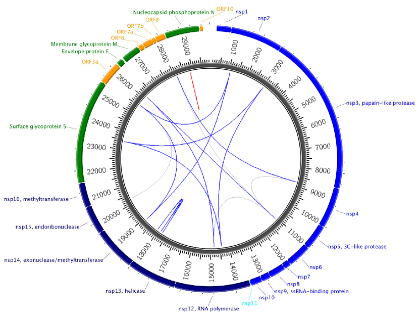
Figure 2: Top-200 significant pairwise epistasis from the 2020-08-08 data-set between loci in coding regions. Colored lines indicate for top 50s, grey lines top 50-200. Red lines show short-distance links (distance less than or equal to 3 bp) blue lines show links of longer distance. The colourful links are the same pairs as listed in Table 1. Analogous circos plots for the 2020-05-02 data set is shown in Appendix L, and for the 2020-04-01 and 2020-04-08 data-sets on the GitHub repository Zeng (2020).

Table 1: Significant links with rank within top-200s between pairwise loci for the 2020-08-08 data-set.

Rank	Locus 1	mutation	Locus 2	mutation	PLM
	-protein	-type	-protein	-type	score
1	1059-nsp2	C$|$T-non.	25563-ORF3a	G$|$T-non.	1.7191
2	28882-N	G$|$A-syn.	28883-N	G$|$C-non.	1.4996
3	28881-N	G$|$A-non.	28882-N	G$|$A-syn.	1.4816
4	28881-N	G$|$A-non.	28883-N	G$|$C-non.	1.4783
5	8782-nsp4	C$|$T-syn.	28144-ORF8	T$|$C-non.	1.4471
9	14805-nsp12	C$|$T-syn.	26144-ORF3a	G$|$T-non.	1.1392
12	3037-nsp3	T$|$C-syn.	14408-nsp12	T$|$C-non.	1.0291
13	18877-nsp14	C$|$T-syn.	25563-ORF3a	G$|$T-non.	1.0131
14	3037-nsp3	T$|$C-syn.	23403-S	G$|$A-non.	1.0114
17	14408-nsp12	T$|$C-non.	23403-S	G$|$A-non.	0.9917
21	1059-nsp2	C$|$T-non.	18877-nsp14	C$|$T-syn.	0.9197
26	17858-nsp13	A$|$G-non.	18060-nsp14	C$|$T-syn.	0.8624
27	17747-nsp13	C$|$T-non.	17858-nsp13	A$|$G-non.	0.8553
36	17747-nsp13	C$|$T-non.	18060-nsp14	C$|$T-syn.	0.7780
47	11083-nsp6	G$|$T-non.	26144-ORF3a	G$|$T-non.	0.7340
63	20268-nsp15	A$|$G-syn.	25563-ORF3a	G$|$T-non.	0.6474
134	11083-nsp6	G$|$T-non.	14805-nsp12	C$|$T-syn.	0.5040
147	11083-nsp6	G$|$T-non.	28144-ORF8	T$|$C-non.	0.4928
168	8782-nsp4	C$|$T-syn.	11083-nsp6	G$|$T-non.	0.4770

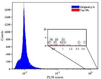
Figure 3: Histograms of PLM scores for (a) original 2020-08-08 data-set, (b) a phylogenetic randomized sample and (c) a profile randomized sample. The blue bars for all scores while the red ones for top-50 largest scores. Red arrows in (a) indicate links listed in Table 3. The largest PLM score is pointed to by red arrows for random samples in (b) and (c). None of them is located inside a coding region, and none of them appear in Table 1 and Table 3.

Table 2: Top 200s that appeared (with an appearance ratio $\geq 10\%$ ) in samples with phylogeny randomization strategy based on the 2020-08-08 data-set. 50 phylogeny samples are considered in total.

Hit	Locus 1	mutation	Locus 2	mutation
ratio	-protein	-type	-protein	-type
14%	28881-N	G$|$A-non.	28882-N	G$|$A-syn.
16%	28881-N	G$|$A-non.	28883-N	G$|$C-non.
20%	28882-N	G$|$A-syn.	28883-N	G$|$C-non.
22%	3037-nsp3	T$|$C-syn.	14408-nsp12	T$|$C-non.
20%	3037-nsp3	T$|$C-syn.	23403-S	G$|$A-non.
34%	14408-nsp12	T$|$C-non.	23403-S	G$|$A-non.

Table 3: Potentially significant epistatic links in Table 1, and corresponding amino acid mutations

Rank	Locus 1-	amino acid	Locus 2-	amino acid
	protein	mutation	protein	mutation
1	1059-nsp2	T85I(T)	25563-ORF3a	Q57H(Q)
5	8782-nsp4	S76S(S)	28144-ORF8	L84S(L)
9	14805-nsp12	T455I(Y)	26144-ORF3a	G251V(G)
21	1059-nsp2	T85I(T)	18877-nsp14	L280L(L)
26	17858-nsp13	T541C(Y)	18060-nsp14	L7L(L)
27	17747-nsp13	P504L(P)	17858-nsp13	T541C(Y)
36	17747-nsp13	P504L(P)	18060-nsp14	L7L(L)
47	11083-nsp6	L37F(L)	26144-ORF3a	G251V(G)

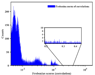
Figure 4: Frobenius norm of pairwise correlations between loci for the original 2020-08-08 data-set. The score pointed by the red arrow corresponds to the link of 1059-25563.

Table 4: Top-10 links found by correlation analysis in the coding region for the data-set till 2020-08-08.

Rank	Locus 1	Locus 2	Frobenius
	-protein	-protein	Score
455	3037-nsp3	23403-S	0.3844
458	3037-nsp3	14408-nsp12	0.3842
460	14408-nsp12	23403-S	0.3837
581	28882-N	28883-N	0.3609
584	28881-N	28883-N	0.3603
585	28881-N	28882-N	0.3603
1071	1059-nsp2	25563-ORF3a	0.2821
2394	8782-nsp4	28144-ORF8	0.1803
3969	23403-S	28144-ORF8	0.1487
3980	3037-nsp3	28144-ORF8	0.1486

Appendix A Quasi-linkage equilibrium (QLE) and its range of validity

Quasi-linkage equilibrium was discovered by Kimura Kimura (1956) and investigated more recently by Neher and Shraiman Neher and Shraiman (2009, 2011). The connection to inference was made in Gao et al. (2019) where the theory was also extended from Boolean variables (bi$-$allelic loci) to categorical data (arbitrary number of alleles per locus).

QLE refers to the state of a population comprising $N$ individuals. That can be characterized by the list of genotypes present, or equivalently by an empirical probability distribution

$$P^{(e)}(\mathbf{\sigma})=\frac{1}{N}\sum_{s}\mathbf{1}_{\mathbf{\sigma},\mathbf{\sigma}^{(s)}}$$ (8)

In above $\mathbf{\sigma}^{(s)}$ is the genotype of individual $(s)$ and $\mathbf{1}_{\mathbf{\sigma},\mathbf{\sigma}^{(s)}}$ means that individuals of genotype $\mathbf{\sigma}$ are counted in the sum. Each genotype can hence appear zero, once or many times; if more than zero such a group is referred to as a clone, and if more than once a multi-individual clone, or a proper clone. We will in the following for simplicity take $N$ to be fixed. In QLE there are few proper clones, i.e. most individuals in the population have a unique genotype.

In models of evolution where the QLE concept is pertinent populations change in time due to mutations, recombination, fitness and genetic drift. Mutation and recombination are random events characterized by average rates. Fitness is the propensity of an individual to have offspring in the next generation and genetic drift is the randomness associated with this process. The population history is hence given by a sequence of empirical probability distributions indexed by time ($t$), $P^{(e)}(\mathbf{\sigma},t)$.

The development in time can alternatively be formulated on the level of ensemble probability distributions. In general that will be the time-dependent joint probability distributions of $N$ genomes $P_{N}(\mathbf{\sigma}_{1},\mathbf{\sigma}_{1},\ldots,\mathbf{\sigma}_{N},t)$. Mutation, fitness and genetic drift act on each genotype in the population separately. They can thus be formulated for the marginalization $P_{N}$ to a one-genome ensemble probability distribution $P(\mathbf{\sigma},t)$. Recombination acts on two genomes at a time. They can thus be formulated on the level of two-genome ensemble probability distributions $P_{2}(\mathbf{\sigma}_{1},\mathbf{\sigma}_{2},t)$.

QLE is characterized by multi-genome distribution functions factorizing i.e. by

$$P(\mathbf{\sigma}_{1},...,\mathbf{\sigma}_{N})\approx P(\mathbf{\sigma}_{1})...P(\mathbf{\sigma}_{N}).$$ (9)

As a consequence, evolution can be considered on the level of one-genome ensemble probability distributions only. The resulting equations have been written out and discussed in Neher and Shraiman (2009, 2011); Gao et al. (2019); Zeng and Aurell (2020) and are structurally similar to the Boltzmann equation in gas kinetics, where recombination plays the role of a collision term. It is a reasonable picture to consider the list of $N$ genotypes given by $P^{(e)}$ as $N$ samples from $P$. However, as follows from above, the relation between the two distributions is not direct: $P^{(e)}$ changes according to a stochastic and frequency-independent evolution law while $P$ obeys a deterministic nonlinear partial differential equation.

The form of QLE, for only bi-allelic loci and only one-locus fitness terms (additive fitness) and two-loci fitness terms (epistatic fitness) is that of the Ising model of statistical mechanics i.e. for a genome $\mathbf{\sigma}=(s_{1},\ldots,s_{L})$

$$P(\mathbf{\sigma})=\frac{1}{Z}\exp\left(\sum_{i}h_{i}s_{i}+\sum_{ij}J_{ij}s_{i}s_{j}\right)$$ (10)

In above both sums go over the loci of variability on the genome. In some applications they could be all or almost all positions, but in the application to SARS-CoV-2 genomes they are but a small fraction. At most genomic positions all samples carry the same variant; those positions are not included in the sums in (10) which focus on the variable portions. Further, $s_{i}=1$ in (10) encodes one of the alleles (typically the major allele) and $s_{i}=-1$ encodes the other allele (typically the minor allele), $h_{i}$ and $J_{ij}$ parametrize the distribution and $Z$ is a normalization constant (partition function). The extension of the above to more the bi-allelic loci (”Potts genomes”) is given in Gao et al. (2019), and restated in main body of the paper, Eqs. (3) and (4). Although we in this work only find properties of almost bi-allelic pairs of loci, the intermediate analysis allows multi-allelic states (see below).

Known sufficient conditions for QLE are that recombination is sufficiently high everywhere compared to selection, and mutation rate is non-zero. The part of the argument concerning recombination was made on the physical level of rigor in Neher and Shraiman (2011), by estimating terms in a Taylor series in inverse recombination rate. The part of the argument concerning mutation is implicit in Neher and Shraiman (2011), and based on the observation that without mutations, the most fit genotype will eventually take over in a finite population. This means that mutation must be non-zero, as otherwise QLE will only be a (possibly long-lived) transient Zeng and Aurell (2020). On a qualitative level the argument for QLE is analogous to the accuracy of Boltzmann equation and the stationary state being of Gibbs-Boltzmann type when collision rate is high enough Gao et al. (2019).

Many realistic models encode that recombination acts more weakly between closely spaced loci. Taken at face value, the conditions in Neher and Shraiman (2009, 2011); Gao et al. (2019) would then imply that the conditions for QLE can be at hand for loci sufficiently far apart on the genome, but not for closely spaced loci. A quantitative theory of this effect as it relates to QLE is at this point lacking. Numerical results in Neher and Shraiman (2009, 2011) showed that the characteristics of QLE may be present, and numerical results in Zeng and Aurell (2020) showed that QLE can be used for inference in this setting.

Necessary conditions for the validity of QLE are at this point not known. It may be that states similar to QLE can also be found in other parameter ranges than at high recombination. An argument in favor is the recent in silico result in Zeng et al. (2020) where a modified form of QLE inference was shown to work also for moderate recombination, given instead high enough mutation rates.

Appendix B Approximate inference in QLE

QLE gives quantitative relations between evolutionary dynamics and distributions over genotypes in a population. In this section we state and briefly describe what these relations are, and how we use them in this work.

We are only here concerned with the most important relation, which connects the parameters $J_{ij}$ in (10) to parameters describing how fitness and recombination shape the population. Fitness is here taken as a propensity of a genotype to propagate in the next generation. It is parametrized as

$$F(\mathbf{\sigma})=\sum_{i}f_{i}s_{i}+\sum_{ij}f_{ij}s_{i}s_{j}$$ (11)

where the $f_{i}$ and $f_{ij}$ are respectively the additive and the epistatic components of fitness and the genome is assumed bi-allelic as in (10); for the extension to multi-allelic sites see Gao et al. (2019). The meaning of (11) is that individuals with higher total fitness (higher $F(\mathbf{\sigma})$) will have higher expected number of offspring. Recombination is described by an overall rate $r$ and a locus-pair-dependent quantity $c_{ij}$ which is the probability that alleles at loci $i$ and $j$ are inherited from different parents if a recombination event has taken place. In many cases it is reasonable to assume that this quantity is small (close to zero) when $i$ and $j$ lie sufficiently closely on the genome, and approximate $\frac{1}{2}$ if they are distant.

The relation first found by Kimura for a two-locus problem is

$$J_{ij}=\frac{f_{ij}}{r\cdot c_{ij}}$$ (12)

In a world abundant in sequenced genomes the left hand side of above can be inferred from samples. It is thus what can be considered known, while what causes it, $f_{ij}$ and the influence of recombination, are quantities not known directly. It is therefore useful to re-state (12) as

$$f^{*}_{ij}=J^{*}_{ij}\cdot rc_{ij}$$ (13)

where the star indicates that these quantities are inferred from data.

Finally, for sites far enough apart on the genome the above can be summarized that epistatic term in fitness ($f_{ij}$) is proportional to pair-wise term in the distribution ($J_{ij}$). A ranking of pairs in descending order of $J_{ij}$ is hence also a ranking of pairs in descending order of epistatic fitness, if closely spaced pairs are excluded. This is hence the theoretical basis of the analysis in the main body of the paper, where we rank pairs as to the values of $J^{*}_{ij}$, as inferred from samples. The extension of the above to Potts genomes (multi-allelic states) is given in Gao et al. (2019) and Zeng and Aurell (2020).

Appendix C Methods of DCA

Determining the coefficients in a distribution of the type (10) from data has been called a problem of inference in exponential families in statistics Wainwright and Jordan (2008), an inverse Ising problem in statistical physics Roudi et al. (2009); Aurell and Ekeberg (2012); Nguyen et al. (2017) and direct coupling analysis (DCA) in computational biology Morcos et al. (2011); Cocco et al. (2018). The benchmark method for such problems is maximum likelihood (ML). This is built from the assumption that $N$ observed genotypes are independent draws from a distribution of type (10). The logarithm of the probability of the joint distribution (log-likelihood) is then

$${\cal L}\left(\{h_{i}\},\{J_{ij}\}\right)=\sum_{i}h_{i}\left(\frac{1}{N}\sum_{s}s_{i}^{s}\right)+\sum_{ij}J_{ij}\left(\frac{1}{N}\sum_{s}s_{i}^{s}s_{j}^{s}\right)-\log Z$$ (14)

The averages on the right hand side multiplying $h_{i}$ and $J_{ij}$ are empirical averages. Since these are the only properties of the samples which enter into the log-likelihood they are sufficient statistics for ML inference. The partition function ($Z$) is computationally difficult to evaluate, and a large number of other inference procedures to circumvent this problem are therefore widely used, reviewed recently in Cocco et al. (2018); Nguyen et al. (2017).

One family of widely used approaches is variational methods. This is based on minimizing the distance between the empirical distribution and a suitable trial distribution, in practice mostly factorized distribution Wainwright and Jordan (2008), although later distribution of the type (10) have also been used Nguyen et al. (2017) (and references therein). The most widely used variational inference is naive mean-field which is equivalent to treating the Ising (or Potts) distribution over discrete variables as if it were a Gaussian distribution over continuous variables. While naive mean-field inference was the basis for important advances in protein structure prediction Morcos et al. (2011); Söding (2017), it has more recently been overtaken by pseudo-likelihood maximization (PLM) Besag (1975); Ravikumar et al. (2010); Aurell and Ekeberg (2012); Nguyen et al. (2017); Cocco et al. (2018). PLM is the DCA method used in this work. The principles are described in Materials & Methods section of the main body of the paper, text around Eqs. (5) and (6). The implementation of PLM which we have used (also called PLM), due to Chen-Yi Gao Gao et al. (2018) is available on Gao (2018).

Appendix D Phylogenetic randomization of DCA: principles

This section describes the two means of phylogenetic randomization used in the main paper. A full-length technical description of both methods is available (from co-author ERH) at Horta and Weigt (2020).

Profile randomization: This approach is built on the principle of randomizing the input multi-sequence alignment (MSA) by conserving the single-columns statistics $w_{i}(\sigma)$, for all sites $i=1,...,L$ and all nucleotides or gaps $\sigma\in\left\{-,N,A,C,G,T\right\}$. This is done by independent columns shuffling which destroys all kinds of correlations (both coevolutionary ones and phylogenetic ones) present in the alignment, only the residue conservation patterns of the original MSA are preserved. The randomized sequences become an independently and identically distributed sample from the profile model

$$P(\sigma_{1},...,\sigma_{L})=\prod_{i=1}^{L}w_{i}(\sigma_{i}).$$

Profile randomization hence serves to verify that the effects found are not due to random sampling. An alternative way to reach the same goal, and high-lighted in the main body of the paper, is to repeat the analysis with successively larger collections of genomes obtained from using successively later cut-off dates.

Phylogeny randomization: This more advanced approach is built on the principle of randomizing the input MSA preserving both single columns statistics and pairwise Hamming distances between sequences representing the genotypes. This method was first presented in detail in Horta and Weigt (2020). Computational methods to infer phylogeny which rely on such pair-wise Hamming distances would by design be insensitive to phylogeny randomization, i.e. the give the same result as using input MSA. Phylogeny randomization hence serves to distinguish co-variation between loci due to phylogeny (inheritance) from co-variation due to co-evolution (epistasis).

The method is initialized with an alignment resulting from the “profile” randomization, eliminating all preexisting correlations, to then start a simulated annealing based method to construct a sequence alignment with inter-sequences distances of the original MSA as target. Single variables $\sigma^{(i)}_{k}$ are permuted in the following way: at each move t, a column $k$ and two rows $m$ and $n$ are chosen at random, and an attempt to exchange $\sigma^{(m)}_{k}$ and $\sigma^{(n)}_{k}$ is made. The probability of the exchange to take place is the Metropolis-Hastings acceptance probability:

$$P_{acc}(t,\beta)=\min\left(1,\exp\left(\beta\left(||\bm{h}^{t}-\bm{h}_{target}||-||\bm{h}^{t-1}-\bm{h}_{target}||\right)\right)\right)$$ (15)

where $\bm{h}^{t-1}$ and $\bm{h}^{t}$ are the Hamming distance matrices of the current alignment before and after the exchange, $\bm{h}_{target}$ the Hamming distance matrix corresponding to the original alignment, $||\dots||$ stands for the Frobenius matrix norm, and $\beta$ is an inverse temperature parameter. Thus, a move is more likely to be accepted if it makes the Hamming distance matrix of the alignment closer to that of the target. Parameter $\beta$ is initialized at a low value and then slowly increased as more moves are made, When $\beta$ goes to infinity and annealing has proceeded slowly enough $\bm{h}\rightarrow\bm{h}_{target}$.

This procedure never changes the single site statistics of the target alignment, since exchanges are made inside one column. On other hand all the epistatic correlations are destroyed. If we assume that the target Hamming distance matrix is a measure of the phylogenetic information in the original MSA, as is done in several tree building methods (distance-based methods) Felsenstein (2004); Saitou and Nei (1987), then we expect that resulting alignment present this hierarchical signal.

Appendix E Phylogenetic randomization of DCA: results and visualization

Starting from the filtered MSA for the 2020-08-08 data-set, we apply the two randomization strategies described above. For profile randomization 50 samples are generated and the PLM procedure is implemented to infer the epistasis between pairwise loci.

As stated in main body of the paper, for further analysis we only retained pairs where both the inferred loci are located in the coding region and the first and second prevalent nucleotides of these loci in the analyzed data-set are entries in {A,C,G,T} . We observed no such pairs in the top-200 PLM scores, for any profile randomized samples. Therefore, the examined ranks of PLM scores are extended to top-2000s. In Fig. 6, the inferred top-2000 epistasis for each sample are shown. There are 24 out of 50 samples which contain interactions found by PLM. However, as they all have low rank, none of these links show up in Table 1 in the main body of the paper.

For phylogeny randomization we also generated 50 random samples. The inferred epistasis for these samples are shown in Fig. 7 and continued in Fig. 8. Unlike profile strategy, a subset of the putative epistatic links of Table 1 in the main body of the paper also show up after phylogeny randomization. This subset of predictions is listed in Table 2 in the main body of the paper, and has been eliminated in the list of retained predictions in Table 3.

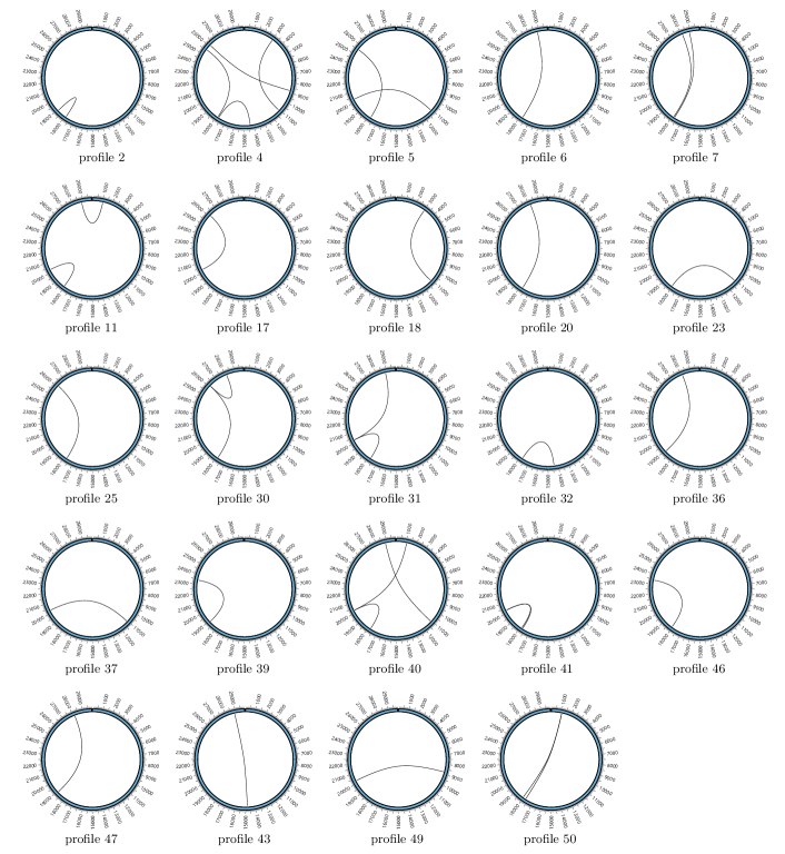
Figure 6: Links within top-2000 PLM scores of samples with profile randomization. The links located in coding regions and terminals have mutations excluding gaps and ’N’s are retained in these circos plots. There are 24 out of 50 samples contain links. However, all of these are ranked low starting from the original MSA, and none of them show up in Table 1 in the main body of the paper.

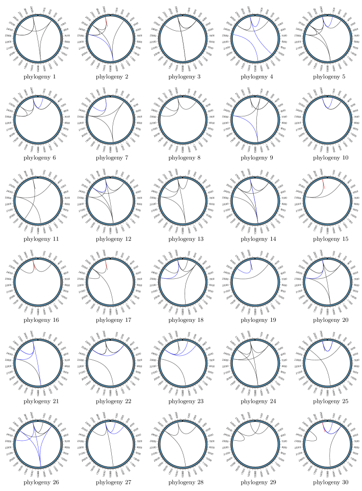
Figure 7: Links within top-200 PLM scores of the 1st to the 30th samples with phylogenetic randomization. The links located in coding regions are retained in these circos plots. Each phylogenetic sample contains interactions effects with a rank cut-off threshold of 200. Blue shows links with lengths $d_{ij}$ longer than 3 nucleotide. Red shows links with $d_{ij}\leq 3nt$ for links with rank in top-50s. Black shows links with $d_{ij}\leq 3nt$ for links with rank in top 51-200.

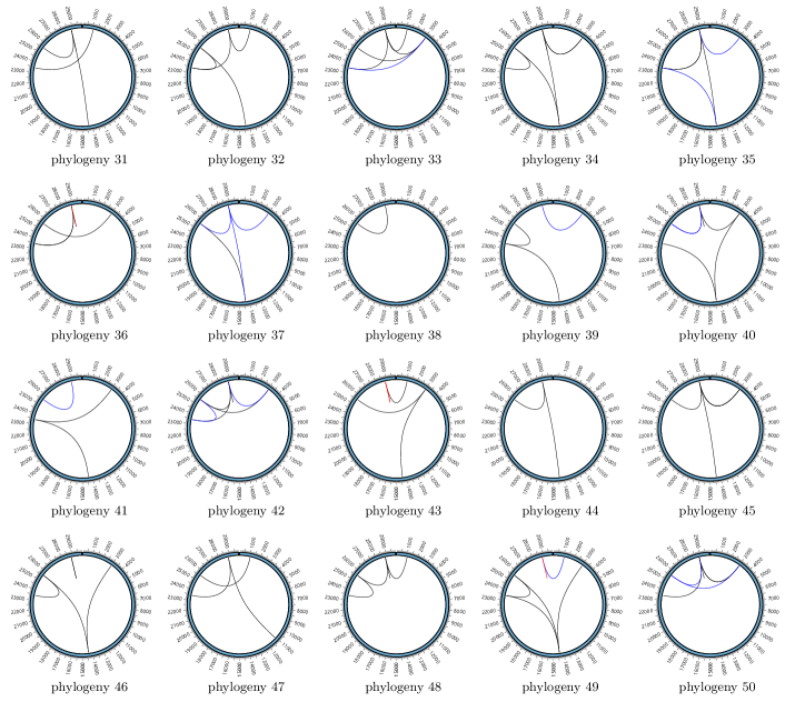
Figure 8: Links within top-200 PLM scores of the 31st to 50th samples with phylogenetic randomization.

Appendix F Robustness as to thresholds

In the analysis in main body of the paper, the following criteria are used for pre-filtering of the MSA. First, if in one locus the same nucleotide is found in a percentage $P_{major}\geq 96.5\%$ of the samples, or if the sum of the percentages of A, C, G and T at this position is $P_{sum}\leq 20\%$, then this locus will be deleted. The inferred epistasis effects are found to be sensitive to $P_{major}$ at a certain locus but not to $P_{sum}$. We chose the criterion $P_{major}\geq 96.5\%$ to keep consistency with earlier obtained results from the dataset of 2020-05-02 (presented below). For that earlier (smaller) dataset, the same results are obtained also with less permissive thresholds. To check the influence of $P_{major}$, we performed PLM inference over the 2020-08-08 dataset with $P_{major}=90\%$ and $P_{major}=95\%$ respectively. The inferred epistasis for these two $P_{major}$s are shown in the left and right panel of Fig. 9 respectively. By increasing the threshold, more epistasis effects are inferred. In summary, most of the links presented with lower $P_{major}$ remain in the results with higher thresholds.

For the visualization of epistasis effects, we focus on links with both terminals located in coding regions and mutation types are gaps and ’N’s excluded. As shown in Fig. 9, different colors mean links with different ranks. Red (links with terminals located close to each other) and blue (the terminals are far away from each other) are for the epistasis links with ranks less than 50 while grey for links with ranks within 51 to 200. Both panels clearly show that with PLM method, most significant links are in top-50s. This indicates that the choice of visualization threshold are reasonable in the presentation of epistasis effects.

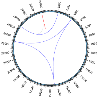
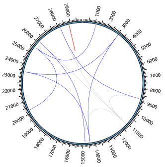
Figure 9: Top-200 significant pairwise epistasis from the 2020-08-08 data-set. Upper: the filtering threshold is 90% (for a given locus, if the percentage of a certain main nucleotide (A, C, G, T, -, N) exceeds the threshold, this locus will be deleted.); Lower: the threshold value is 95%. Only epistatic links with both terminals located in the coding region and no gaps and ’N’s included in mutations are presented here. Colored lines indicate for top 50s, grey for links with ranks in top 50-200s. Red lines show short-distance links ($\leq$ 3 bp) blue lines show links of longer distance.

Appendix G Different quantifications of correlations

The correlation (co-variance) of two Boolean variables is given by one real number. If the Boolean variables are represented as spin variables $s_{i}$ and $s_{j}$ taking values $1$ and $-1$, this number is the physical correlation $\chi_{ij}=\langle s_{i}s_{j}\rangle-\chi_{i}\chi_{j}$, where $\chi_{i}=\langle s_{i}\rangle$ and $\chi_{j}=\langle s_{j}\rangle$. Since every joint distribution on two Boolean variables can be written $p(s_{i},s_{j})=\frac{1}{4}\left(1+\chi_{i}s_{i}+\chi_{j}s_{j}+(\chi_{i}\chi_{j}+\chi_{ij})s_{i}s_{j}\right)$ with marginals $p(s_{i})=\frac{1}{2}\left(1+\chi_{i}s_{i}\right)$ and $p(s_{j})=\frac{1}{2}\left(1+\chi_{j}s_{j}\right)$, the contrast is

$$c(s_{i},s_{j}) = \frac{p(s_{i},s_{j})}{p(s_{i})p(s_{j})}$$ (16)

$$= \frac{1+\chi_{i}s_{i}+\chi_{j}s_{j}+(\chi_{i}\chi_{j}+\chi_{ij})s_{i}s_{j}}{1+\chi_{i}s_{i}+\chi_{j}s_{j}+\chi_{i}\chi_{j}s_{i}s_{j}}~{}.$$

The mutual information (MI), recently used in genome-scale epistasis analysis in Pensar et al. (2019), is the expected log-contrast

$$I_{ij} = \sum_{s_{i},s_{j}}p(s_{i},s_{j})\log c(s_{i},s_{j})$$

$$= \frac{1}{4}\left((1+\chi_{i}+\chi_{j}+a_{ij})\log\frac{1+\chi_{i}+\chi_{j}+a_{ij}}{1+\chi_{i}+\chi_{j}+\chi_{i}\chi_{j}}\right.$$

$$+(1-\chi_{i}+\chi_{j}-a_{ij})\log\frac{1-\chi_{i}+\chi_{j}-a_{ij}}{1-\chi_{i}+\chi_{j}-\chi_{i}\chi_{j}}$$

$$+(1+\chi_{i}-\chi_{j}-a_{ij})\log\frac{1+\chi_{i}-\chi_{j}-a_{ij}}{1+\chi_{i}-\chi_{j}-\chi_{i}\chi_{j}}$$

$$+\left.(1-\chi_{i}-\chi_{j}+a_{ij})\log\frac{1-\chi_{i}-\chi_{j}+a_{ij}}{1-\chi_{i}-\chi_{j}+\chi_{i}\chi_{j}}\right)~{}.$$

with $a_{ij}=\chi_{i}\chi_{j}+\chi_{ij}$.
For given magnetizations ($\chi_{i}$ and $\chi_{j}$), correlations and mutual information of Boolean variables are hence in one-to-one correspondence. In particular, zero correlation implies zero MI. For categorical data (more than two states per variable), correlation is conveniently defined as a matrix

$$f_{ij}(a,b)=\langle\mathbf{1}_{s_{i},a}\mathbf{1}_{s_{j},b}\rangle-f_{i}(a)f_{j}(b)$$ (18)

where $f_{i}(a)=\langle\mathbf{1}_{s_{i},a}\rangle$ and $f_{j}(b)=\langle\mathbf{1}_{s_{j},b}\rangle$. Mutual information is defined in the same way as in (G), except that the sums go over the ranges of indices $a$ and $b$. Frobenius norm (or score) of a correlation matrix is defined as

$$s_{ij}=\sqrt{\sum_{a,b}f_{ij}^{2}(a,b)}$$ (19)

Mutual information and Frobenius norm of correlations of categorical variables are not generally related. It could therefore be the case that the information Fig. (3) and Table 4 in main body of the paper would be different if the assessment would be done for mutual information. Fig. 10 and Table 5 show that this is substantially not the case.

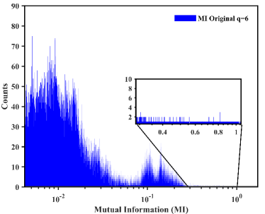
Figure 10: Distribution of Mutual information (MI) between pairwise loci for the original data-set with cut-off date 2020-08-08. The score pointed by the red arrow corresponds to the link with most significant score (1059 to 25563) by PLM analysis.

Table 5: Top-10 significant links found by mutual information (MI) analysis in the coding region for the dataset with cut-off date 2020-08-08.

Rank	Locus 1 -	Locus 2 -	Mutual
	protein	protein	Information
782	28882-N	28883-N	0.5752
792	28881-N	28882-N	0.5698
794	28881-N	28883-N	0.5689
824	3037-nsp3	23403-S	0.5552
836	3037-nsp3	14408-nsp12	0.5478
840	14408-nsp12	23403-S	0.5455
1643	1059-nsp2	25563-ORF3a	0.3261
1775	8782-nsp4	28144-ORF8	0.3118
18484	17858-nsp13	18060-nsp14	0.1705
19364	17747-nsp13	17858-nsp13	0.1679

Another way to quantify interdependence between two random variables is the $p$-value of Fisher’s exact test Wikipedia Community (2020), recently used in the present context in Cui et al. (2020). If in $n$ samples in total outcome $ab$ is found $n_{ab}$ time then the $p$-value of Fisher’s exact test is the probability that these outcomes would have been observed in independent draws of independently distributed variables. For Boolean variables that has the exact expression

$$p_{ij}(n,\{n_{ab}\})=\frac{(n_{11}+n_{1-1})!\cdot(n_{-11}+n_{-1-1})!\cdot(n_{11}+n_{-11})!\cdot(n_{1-1}+n_{-1-1)})!}{n_{11}!\cdot n_{-11}!\cdot n_{1-1}!\cdot n_{-1-1}!\cdot n!}$$ (20)

In the limit of many samples $n_{ab}=n\cdot p_{ij}(a,b)$ almost surely, and by Stirling’s formula

$$\log p_{ij}(n) \approx n\big{(}(p_{ij}(1,1)+p_{ij}(1,-1))\log(p_{ij}(1,1)+p_{ij}(1,-1))+(p_{ij}(-1,1)+p_{ij}(-1,-1))\log(p_{ij}(-1,1)+p_{ij}(-1,-1))$$

$$+ (p_{ij}(1,1)+p_{ij}(-1,1))\log(p_{ij}(1,1)+p_{ij}(-1,1))+(p_{ij}(1,-1)+p_{ij}(-1,-1))\log(p_{ij}(1,-1)+f_{ij}(-1,-1))$$

$$- p_{ij}(1,1)\log p_{ij}(1,1)-p_{ij}(1,-1)\log p_{ij}(1,-1)-p_{ij}(-1,1)\log p_{ij}(-1,1)-p_{ij}(-1,-1)\log p_{ij}(-1,-1)\big{)},$$

which is mutual information, up to a factor $-n$. In a more general setting, this result follows from Sanov’s lemma in Information Theory. For the data we consider we are always in the range of very large $n$, and Fisher’s exact test therefore does not give additional information.

Appendix H On putative couplings between nsp7 (11843..12091) and nsp8 (12092..12685)

As described above, the set of loci remaining after filtering depends on the percentage of the a major nucleotide $P_{major}$ used as threshold. As the two viral genes nsp7 and nsp8 are known to interact Peng et al. (2020)， we looked for epistatic interactions between loci in these two genes. None appear using the threshold $P_{major}=96.5\%$ employed in the main body of the paper. All loci located in nsp7 and nsp8 are deleted during filtering procedure using this threshold. To nevertheless consider possible epistasis effects within these two regions, we increased the value of $P_{major}$. As $P_{major}$ grows more loci remain after filtering, in all regions, which increases the computational burden. To mitigate this effect, we further filtered the MSA matrix by considering the mutation type of each remaining loci. In the following we have filtered out loci where one of the dominant mutation type are gaps (’-’) or unknown nucleotide (’N’).

With these alternative filtering criteria, we tested values of $P_{major}$ from 97% to 99.9% and found that the loci in nsp7 and nsp8 show up when $P_{major}>99.7\%$. With $P_{major}=99,8\%$, there remains 262 loci and 5,746 unique sequences, from which one locus at position 11916 in nsp7 and two loci at positions 12199 and 12478 in nsp8 are identified. With $P_{major}=99,9\%$, there remains 580 loci and 9525 unique sequences, from which two loci at positions 11916 and 12025 in nsp7 are identified and seven closely positioned loci (12199, 12400, 12478, 12503, 12513, 12534, 12550) in nsp8.

With $P_{major}=99.8\%$, there are 34,191 inferred pairwise epistatic links in total. With $P_{major}=99.9\%$, the number of inferred links is 167,910. The epistasis analysis results provided by PLM procedure are summarized in Table 6. Some significant links with high ranks are included for comparison. Both ranks and PLM scores show that the epistasis effects between nsp7 and nsp8 are much weaker than the significant ones. The ranks for the listed links in Table 6 are obtained without considering gaps ’-’ and not recognized notation ’N’. However, they fit well with the results that including the effects of gaps and ’N’s, at least for the links with the rank of top-50s. In summary, links between loci in genes nsp7 and nsp8 only appear using much more permissive filtering criteria and with much lower rank than the top-200 listed in Table 1 in the main body of the paper.

Table 6: Links between loci in genes nsp7 and nsp8 obtained after the modified filtering procedure applied to the 2020-08-08 data set. Loci without gaps ’-’, without not recognized ’N’ and satisfying permissive threshold criterion $P_{major}=99.8\%$ and $P_{major}=99.9\%$ have been retained and reported here.

Locus 1	mutation	Locus 2	mutation	PLM score	Rank	PLM score	Rank
-protein	-type	-protein	-type	$P_{major}=99.8\%$		$P_{major}=99.9\%$
1059-nsp2	C$|$T-non.	25563-ORF3a	G$|$T-non.	1.9526	3	2.0365	1
8782-nsp4	C$|$T-syn.	28144-ORF8	T$|$C-non.	1.4479	6	1.9739	6
17747-nsp13	C$|$T-non.	17858-nsp13	A$|$G-non.	0.8553	27	1.0522	22
17858-nsp13	T$|$C-non.	18060-nsp14	C$|$T-syn.	0.8624	26	0.9787	27
17747-nsp13	C$|$T-non.	18060-nsp14	C$|$T-syn.	0.7780	36	0.8529	39
11083-nsp6	G$|$T-non.	14805-nsp12	C$|$T-syn.	0.5040	134	0.7109	58
11916-nsp7	C$|$T-non.	12199-nsp8	A$|$G-syn.	0.0259	19781	0.0113	86504
11916-nsp7	C$|$T-non.	12478-nsp8	G$|$A-non.	0.0211	25861	0.0097	109600
12025-nsp7	C$|$T-syn.	12550-nsp8	G$|$A-syn.			0.0325	20933
12025-nsp7	C$|$T-syn.	12199-nsp8	A$|$G-syn.			0.0264	29496
12025-nsp7	C$|$T-syn.	12534-nsp8	C$|$T-non.			0.0237	35797
12025-nsp7	C$|$T-syn.	12478-nsp8	G$|$A-non.			0.0236	35936
12025-nsp7	C$|$T-syn.	12400-nsp8	C$|$T-syn.			0.0202	48464
11916-nsp7	C$|$T-non.	12400-nsp8	C$|$T-syn.			0.0119	83501
11916-nsp7	C$|$T-non.	12513-nsp8	C$|$T-syn.			0.0117	84562
11916-nsp7	C$|$T-non.	12534-nsp8	C$|$T-non.			0.0110	89102
11916-nsp7	C$|$T-non.	12503-nsp8	T$|$C-non.			0.0106	92834
12025-nsp7	C$|$T-syn.	12513-nsp8	C$|$T-non.			0.0099	103746
11916-nsp7	C$|$T-non.	12550-nsp8	G$|$A-syn.			0.0098	105534
12025-nsp7	C$|$T-syn.	12503-nsp8	T$|$C-non.			0.0098	106633

Table 7: Links between loci in genes nsp10 and nsp14 obtained after the modified filtering procedure applied to the 2020-08-08 data set. Loci without gaps ’-’, without not recognized ’N’ and satisfying permissive threshold criterion $P_{major}=99.8\%$ and $P_{major}=99.9\%$ have been retained and reported here. Only links appears in the filtering by both values of threshold are presented here.

Locus 1	mutation	Locus 2	mutation	PLM score	Rank	PLM score	Rank
-protein	-type	-protein	-type	$P_{major}=99.8\%$		$P_{major}=99.9\%$
1059-nsp2	C$|$T-non.	25563-ORF3a	G$|$T-non.	1.9526	3	2.0365	1
8782-nsp4	C$|$T-syn.	28144-ORF8	T$|$C-non.	1.4479	6	1.9739	6
17747-nsp13	C$|$T-non.	17858-nsp13	A$|$G-non.	0.8553	27	1.0522	22
17858-nsp13	T$|$C-non.	18060-nsp14	C$|$T-syn.	0.8624	26	0.9787	27
17747-nsp13	C$|$T-non.	18060-nsp14	C$|$T-syn.	0.7780	36	0.8529	39
11083-nsp6	G$|$T-non.	14805-nsp12	C$|$T-syn.	0.5040	134	0.7109	58
13216-nsp10	T$|$G-non.	18060-nsp14	C$|$T-syn.	0.0407	10743	0.0201	48930
13216-nsp10	T$|$G-non.	18788-nsp14	C$|$T-non.	0.0258	19879	0.0115	85522
13216-nsp10	T$|$G-non.	18877-nsp14	C$|$T-syn.	0.0222	23695	0.0120	83143

Appendix I On putative couplings between nsp10 (13025..13441) and nsp14 (18040..19620)

As the two viral genes nsp10 and nsp14 are also known to interact Ma et al. (2015); Romano et al. (2020) we looked for epistatic interactions between loci in these two genes, applying the same procedure as above. With $P_{major}=99.8\%$ and $P_{major}=99.9\%$, we show three links between loci located in nsp10 and nsp14 that show up in the filtering MSAs with both values of threshold. The corresponding PLM scores and the rank are given in Table 7. Similarly to the links between loci in nsp7 and nsp8, it has very low rank, as well as low PLM score. In the main body of the paper, where filtering criterion $P_{major}=96.5\%$ is used, these loci are filtered out and do not appear.

Appendix J On putative couplings involving loci in Spike

Table 8: Links involving loci in Spike protein obtained after the filtering procedure described in the main context applied to the 2020-08-08 data set with $P_{major}=96.5\%$.

Locus 1	mutation	Locus 2	mutation	PLM score	Rank
-protein	-type	-protein	-type	$P_{major}=96.5\%$
3037-nsp3	T$|$C-syn.	23403-S	G$|$A-non.	1.0114	14
14408-nsp12	T$|$C-non.	23403-S	G$|$A-non.	0.9917	17
23403-S	G$|$A-non.	25563-ORF3a	G$|$T-non.	0.3440	367
11083-nsp6	G$|$T-non.	23403-S	G$|$A-non.	0.3246	428
23403-S	G$|$A-non.	28144-ORF8	T$|$C-non.	0.3240	430
8782-nsp4	C$|$T-syn.	23403-S	G$|$A-non.	0.3022	522
14805-nsp12	C$|$T-syn.	23403-S	G$|$A-non.	0.2787	672
20268-nsp15	A$|$G-syn.	23403-S	G$|$A-non.	0.2496	964
23403-S	G$|$A-non.	26144-ORF3a	G$|$T-non.	0.2349	1166
23403-S	G$|$A-non.	28881-N	G$|$A-non.	0.2108	1571
23403-S	G$|$A-non.	28882-N	G$|$A-syn.	0.2093	1607
23403-S	G$|$A-non.	28883-N	G$|$C-non.	0.2083	1619
1059-nsp2	C$|$T-non.	23403-S	G$|$A-non.	0.2000	1798
18060-nsp14	C$|$T-syn.	23403-S	G$|$A-non.	0.1603	2844
17858-nsp13	A$|$G-non.	23403-S	G$|$A-non.	0.1532	3077
17747-nsp13	C$|$T-non.	23403-S	G$|$A-non.	0.1392	3618
18877-nsp14	C$|$T-syn.	23403-S	G$|$A-non.	0.1186	4523

D614G in Spike is a well known mutation Korber et al. (2020) of SARS-CoV-2, and has become the most prevalent form in the global pandemic COVID19. This mutation is at position of 23403 with respect to the reference genomic sequence (Wuhan-Hu-1). Through PLM procedure on the whole genomic sequences, we observed two pairwise couplings 3037-23403 and 14408-23403 in top-50 PLM scores. These two pairwise links however showed fairly often in phylogeny randomization tests, and have therefore been interpreted as effects of shared inheritance (phylogeny). In above we show all PLM links involving loci in Spike up to rank 5000, all of them significantly below top-200. A notable observation as shown in Table 8 is that the locus 23403 appears in all these links. As the epistatic inference is built on retaining the links with highest PLM scores that also do not also appear after randomization, none of the entries in Table 8 are retained as predicted epistatic interactions in Table 3 of the main body of the paper.

Appendix K Potential drugs for proteins in Table 3 of the main body of the paper

There are eight proteins listed in Table 3 in main body of the paper. Except ORF3a, all these viral proteins have potential drugs listed in Gordon et al. (2020), sorted by human interactors of these proteins, see Table 9. As indicated in the table, several of these drugs are approved, for different purposes listed in Gordon et al. (2020), while some are still in pre-clinical or clinical trials.

Table 9: Potential drugs for interactors of proteins in Table 3, as listed in Gordon et al. (2020). Approved drugs for any purpose in boldface.

Bait	Interactor(s)	Drug	Status
nsp2	FKBP15	Rapamycinb	Approved
	EIF4E2/H	Zotatifinb	Clinical trials
ORF3a	None in Gordon et al. (2020)	-	-
nsp4	NUPs RAE1	Selinexorb	Approved
ORF8	DNMT1	Azacitidine a	Approved
	LOX	CCT 365623 a	Pre-clinical
	FKBP7/10	Rapamycinb	Approved
	FKBP7, FKBP10	FK-506b	Approved
	PLOD1/2	Minoxidilb	Approved
nsp14	IMPDH2	Merimepodib a	Clinical Trial
	GLA	Migalastat a	Approved
	IMPDH2	Mycophenolic acid a	Approved
	IMPDH2	Ribavirin a	Approved
	IMPDH2	Sanglifehrin A b	Pre-clinical
nsp12	RIPK1	Ponatinib a	Approved
nsp13	PRKACA	H-89 a	Pre-clinical
	MARK3,TBK1	ZINC95559591a	Pre-clinical
	CEP250	WDB002b	Clinical Trial
nsp6	ATP6AP1	Bafilomycin A1 a	Pre-clinical
	SIGMAR1	E-52862a	Clinical trials
	SIGMAR1	PD-144418a	Pre-clinical
	SIGMAR1	RS-PPCCa	Pre-clinical
	SIGMAR1	PB28a	Pre-clinical
	SIGMAR1	Haloperidola	Approved
	SLC6A15	Loratadinea	Approved
	SIGMAR1	Chloroquine b	Approved

^a Entry taken from Gordon et al. (2020), Supplementary Table 4, ”Literature-derived drugs and reagents that modulate SARS-CoV-2 interactors”.
^b Entry taken from Gordon et al. (2020), Supplementary Table 5, ”Expert-identified drugs and reagents that modulate SARS-CoV-2 interactors”.

Appendix L Results from data set until 20200502

As more data accumulates the predictions obtained from DCA may change. In the main body of the paper we show in Fig. 4 that the leading predictions are stable using four different cut-off dates: (April 1, April 8, May 2, August 8).

Here we show as a further robustness test the other figures and tables of the main body of the paper, but for the second largest data set (cut-off date May 2, 2020).

Table 10 presents the top-50 significant links for the 20200502 data set, all of them appear in Table 1 in the main context for the 20200808 data set. Table  11 shows the top 10 significant links provided by the correlation analysis for the 20200502 data, which could be compared with Table 4 in the main body of the paper. The Fig. 11 shows the histogram of PLM scores for the original MSAs (Fig. 11(a)) as well as that for phylogeny (Fig. 11(b)) and profile (Fig. 11(c)) randomization respectively. This plot can be compared with the Fig. 2 in the main context.

Table 10: Top-50 significant epistatic links between loci for the 2020-05-02 data-set. To be compared to Table 1 in main body of paper.

Rank	Locus 1 -	mutation-	Locus 2 -	mutation-	PLM
	protein	type	protein	type	score
1	8782-nsp4	C$|$T-syn.	28144-ORF8	T$|$C-non.	2.0649
2	1059-nsp2	C$|$T-non.	25563-ORF3a	G$|$T-non.	1.9480
3	28882-N	G$|$A-syn.	28883-N	G$|$C-non.	1.9116
4	28881-N	G$|$A-non.	28882-N	G$|$A-syn.	1.8774
5	28881-N	G$|$A-non.	28883-N	G$|$C-non.	1.8594
9	17747-nsp13	C$|$T-non.	17858-nsp13	A$|$G-non.	1.4798
13	11083-nsp6	G$|$T-non.	14805-nsp12	C$|$T-syn.	1.3876
16	3037-nsp3	T$|$C-syn.	23403-S	G$|$A-non.	1.3374
17	3037-nsp3	T$|$C-syn.	14408-nsp12	T$|$C-non.	1.2766
20	14408-nsp12	T$|$C-non.	23403-S	G$|$A-non.	1.2101
22	17858-nsp13	T$|$C-non.	18060-nsp14	C$|$T-syn.	1.1973
29	17747-nsp13	C$|$T-non.	18060-nsp14	C$|$T-syn.	1.1392

Table 11: Top-10 significant links found by correlation analysis in the coding region for the data set till 2020-05-02. To be compared to Table 4 in main body of paper.

Rank	Locus 1 -	Locus 2 -	Frobenius
	protein	protein	Score
1	14408-nsp12	23403-S	0.4726
2	3037-nsp3	23403-S	0.4711
3	3037-nsp3	14408-nsp12	0.4706
492	1059-nsp2	25563-ORF3a	0.2894
570	8782-nsp4	28144-ORF8	0.2803
776	28882-N	28883-N	0.255
779	28881-N	28882-N	0.2543
782	28881-N	28883-N	0.2542
1309	14408-nsp12	25563-ORF3a	0.2086
1044	23403-S	25563-ORF3a	0.2081

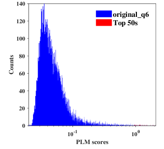
Figure 11: Histograms of PLM scores for (a) 2020-05-02 data-set, (b) a phylogeny randomized sample and (c) a profile randomized sample. The blue bars for all scores while the red ones for top-50 largest scores. Red arrows in (a) indicate links listed in Table 3, with the 29th link almost overlapping with the 22nd. The largest PLM score is pointed to by red arrows for random samples in (b) and (c). None of them is located inside a coding region, and none of them appear in Table 10 and Table 3 in the main context.

References

- World Health Organization (2020) World Health Organization, “Coronavirus disease (covid-19) pandemic,” (2020), accessed September 28, 2020.
- Moritz et al. (2020) K. Moritz, Y. Chia-Hung, G. Bernardo, W. Chieh-Hsi, K. Brennan, P. D. M., du Plessis Louis, F. N. R., L. Ruoran, H. W. P., B. J. S., L. Maylis, V. Alessandro, T. Huaiyu, D. Christopher, P. O. G., and S. S. V., Science 368, 493 (2020).
- Salje et al. (2020) H. Salje, C. T. Kiem, N. Lefrancq, N. Courtejoie, P. Bosetti, J. Paireau, A. Andronico, N. Hozé, J. Richet, C.-L. Dubost, et al., Science (2020).
- Shu and McCauley (2017) Y. Shu and J. McCauley, Eurosurveillance 22 (2017).
- Pachetti et al. (2020) M. Pachetti, B. Marini, F. Benedetti, F. Giudici, E. Mauro, P. Storici, C. Masciovecchio, S. Angeletti, M. Ciccozzi, R. C. Gallo, D. Zella, and R. Ippodrino, J Transl Med. 18, 179 (2020).
- Lai and Cavanagh (1997) M. M. Lai and D. Cavanagh, Adv Virus Res 48, 1‐100 (1997).
- Graham and Baric (2010) R. L. Graham and R. S. Baric, Journal of Virology 84, 3134 (2010).
- Gribble et al. (2020) J. Gribble, A. J. Pruijssers, M. L. Agostini, J. Anderson-Daniels, J. D. Chappell, X. Lu, L. J. Stevens, A. L. Routh, and M. R. Denison, “The coronavirus proofreading exoribonuclease mediates extensive viral recombination,” bioRxiv (2020).
- Li et al. (2020a) X. Li, E. E. Giorgi, M. H. Marichannegowda, B. Foley, C. Xiao, X.-P. Kong, Y. Chen, S. Gnanakaran, B. Korber, and F. Gao, Science Advances (2020a).
- Kimura (1965) M. Kimura, Genetics 52, 875 (1965).
- Neher and Shraiman (2009) R. A. Neher and B. I. Shraiman, Proc. Natl. Acad. Sci. 106, 6866 (2009).
- Neher and Shraiman (2011) R. A. Neher and B. I. Shraiman, Rev. Mod. Phys. 83, 1283 (2011).
- Gao et al. (2019) C.-Y. Gao, F. Cecconi, A. Vulpiani, H.-J. Zhou, and E. Aurell, Phys. Biol. 16, 026002 (2019).
- Zeng and Aurell (2020) H.-L. Zeng and E. Aurell, Phys. Rev. E 101, 052409 (2020).
- Morcos et al. (2011) F. Morcos, A. Pagnani, B. Lunt, A. Bertolino, D. S. Marks, C. Sander, R. Zecchina, J. N. Onuchic, T. Hwa, and M. Weigt, PNAS 108, E1293 (2011).
- Cocco et al. (2018) S. Cocco, C. Feinauer, M. Figliuzzi, R. Monasson, and M. Weigt, Reports on Progress in Physics 81 (2018).
- Shekhar et al. (2013) K. Shekhar, C. F. Ruberman, A. L. Ferguson, J. P. Barton, M. Kardar, and A. K. Chakraborty, Phys. Rev. E 88, 062705 (2013).
- Mann et al. (2014) J. K. Mann, J. P. Barton, A. L. Ferguson, S. Omarjee, B. D. Walker, A. Chakraborty, and T. Ndung’u, PLOS Computational Biology 10, 1 (2014).
- Cheng et al. (2016) R. R. Cheng, O. Nordesjö, R. L. Hayes, H. Levine, S. C. Flores, J. N. Onuchic, and F. Morcos, Molecular Biology and Evolution 33, 3054 (2016).
- de la Paz et al. (2020) J. A. de la Paz, C. M. Nartey, M. Yuvaraj, and F. Morcos, PNAS 117, 5873 (2020).
- Horta et al. (2019) R. Horta, P. Barrat-Charlaix, and M. Weigt, Entropy 21, 1 (2019).
- Forster et al. (2020) P. Forster, L. Forster, C. Renfrew, and M. Forster, PNAS 117, 9241 (2020).
- Khailany et al. (2020) R. A. Khailany, M. Safdar, and M. Ozaslan, Gene reports 19, 100682 (2020).
- Cai et al. (2020) H. Y. Cai, K. K. Cai, and J. Li, Preprints (2020).
- Deng et al. (2020) X. Deng, W. Gu, S. Federman, and et al, “A Genomic Survey of SARS-CoV-2 Reveals Multiple Introductions into Northern California without a Predominant Lineage,” medRxiv (2020).
- Phelan et al. (2020) J. Phelan, W. Deelder, D. Ward, S. Campino, M. L. Hibberd, and T. G. lark, “Controlling the SARS-CoV-2 outbreak, insights from large scale whole genome sequences generated across the world,” biorxiv (2020).
- Sashittal et al. (2020) P. Sashittal, Y. Luo, J. Peng, and M. El-Kebir, “Characterization of SARS-CoV-2 viral diversity within and across hosts,” biorxiv (2020).
- Tang et al. (2020) X. Tang, C. Wu, X. Li, Y. Song, X. Yao, X. Wu, Y. Duan, H. Zhang, Y. Wang, Z. Qian, J. Cui, and J. Lu, National Science Review (2020).
- Zeng (2020) H.-L. Zeng, “hlzeng/FilteredMSASARSCoV2,” Github (2020), https://github.com/hlzeng/Filtered_MSA_SARS_CoV_2.
- Katoh et al. (2017) K. Katoh, J. Rozewicki, and K. D. Yamada, Briefings in Bioinformatics 20, 1160 (2017), https://mafft.cbrc.jp/alignment/server/.
- Kuraku et al. (2013) S. Kuraku, C. M. Zmasek, O. Nishimura, and K. Katoh, Nucleic Acids Research 41, W22 (2013).
- Ekeberg et al. (2014) M. Ekeberg, T. Hartonen, and E. Aurell, J. Comput. Phys. 276, 341 (2014).
- MacLean et al. (2020) O. A. MacLean, R. J. Orton, J. B. Singer, and D. L. Robertson, Virus Evolution 6 (2020).
- Skwark et al. (2017) M. J. Skwark, N. J. Croucher, S. Puranen, C. Chewapreecha, M. Pesonen, Y. Y. Xu, P. Turner, S. R. Harris, S. B. Beres, J. M. Musser, J. Parkhill, S. D. Bentley, E. Aurell, and J. Corander, PLos Genet. 13, e1006508 (2017).
- Schubert et al. (2019) B. Schubert, R. Maddamsetti, J. Nyman, M. R. Farhat, and D. S. Marks, Nat. Microbiol. 4, 328 (2019).
- Cui et al. (2020) Y. Cui, C. Yang, H. Qiu, H. Wang, R. Yang, and D. Falush, eLife 9, e54136 (2020).
- Schneidman et al. (2006) E. Schneidman, M. J. Berry, R. Segev, and W. Bialek, Nature 440, 1007 (2006).
- Russ et al. (2005) W. P. Russ, D. M. Lowery, P. Mishra, M. B. Yaffe, and R. Ranganathan, Nature 437, 579 (2005).
- Socolich et al. (2005) M. Socolich, S. W. Lockless, W. P. Russ, H. Lee, K. H. Gardner, and R. Ranganathan, Nature 437, 512 (2005).
- Nguyen et al. (2017) H. C. Nguyen, R. Zecchina, and J. Berg, Advances in Physics 66, 197 (2017).
- Besag (1975) J. Besag, The Statistician 24, 179 (1975).
- Ravikumar et al. (2010) P. Ravikumar, M. J. Wainwright, and J. D. Lafferty, Ann. Stat. 38, 1287 (2010).
- Aurell and Ekeberg (2012) E. Aurell and M. Ekeberg, Phys. Rev. Lett. 108, 090201 (2012).
- Ekeberg et al. (2013) M. Ekeberg, C. Lövkvist, Y. Lan, M. Weigt, and E. Aurell, Phys. Rev. E 87, 012707 (2013).
- Gao (2018) C.-Y. Gao, “gaochenyi/cc-plm,” Github (2018), http://github.com/gaochenyi/CC-PLM.
- Krzywinski et al. (2009) M. I. Krzywinski, J. E. Schein, I. Birol, J. Connors, R. Gascoyne, D. Horsman, S. J. Jones, and M. A. Marra, Genome Res. 19, 1639 (2009).
- Mandin et al. (2007) P. Mandin, F. Repoila, M. Vergassola, T. Geissmann, and P. Cossart, Nucleic Acids Research 35, 962 (2007).
- Xu et al. (2018) Y. Xu, S. Puranen, J. Corander, and Y. Kabashima, Phys. Rev. E 97, 062112 (2018).
- Horta and Weigt (2020) E. R. Horta and M. Weigt, “Phylogenetic correlations have limited effect on coevolution-based contact prediction in proteins,” bioRxiv (2020).
- Wu et al. (2020) F. Wu, S. Zhao, B. Yu, Y.-M. Chen, W. Wang, Z.-G. Song, Y. Hu, Z.-W. Tao, J.-H. Tian, Y.-Y. Pei, et al., Nature 579, 265 (2020).
- Yoshimoto (2020) F. K. Yoshimoto, Protein J 39, 198 (2020).
- Hosseini and Donald (2020) R. A. Hosseini and M. A. Donald, “Implications of sars-cov-2 mutations for genomic rna structure and host microrna targeting,” (2020).
- Rui et al. (2020) W. Rui, C. Jiahui, G. Kaifu, H. Yuta, Y. Changchuan, and W. Guo-Wei, “Characterizing SARS-CoV-2 mutations in the United States,” (2020).
- Kern et al. (2020) D. M. Kern, B. Sorum, C. M. Hoel, S. Sridharan, J. P. Remis, D. B. Toso, and S. G. Brohawn, “Cryo-EM structure of the SARS-CoV-2 3a ion channel in lipid nanodiscs,” bioRxiv (2020).
- Tan et al. (2005) Y.-J. Tan, P.-Y. Tham, D. Z. L. Chan, C.-F. Chou, S. Shen, B. C. Fielding, T. H. P. Tan, S. G. Lim, and W. Hong, J Virol 79, 10083‐10087 (2005).
- Lu et al. (2006) W. Lu, B.-J. Zheng, K. Xu, W. Schwarz, L. Du, C. K. L. Wong, J. Chen, S. Duan, V. Deubel, and B. Sun, PNAS 103, 12540—12545 (2006).
- Siu et al. (2019) K.-L. Siu, K.-S. Yuen, C. C. no Rodriguez, Z.-W. Ye, M.-L. Yeung, S.-Y. Fung, S. Yuan, C.-P. Chan, K.-Y. Yuen, L. Enjuanes, and D.-Y. Jin, FASEB J 33, 8865‐8877 (2019).
- Ren et al. (2020) Y. Ren, T. Shu, D. Wu, J. Mu, C. Wang, M. Huang, Y. Han, X.-Y. Zhang, W. Zhou, Y. Qiu, and X. Zhou, Cellular and Molecular Immunology 17, 881 (2020).
- Elio et al. (2020) I. Elio, M. Georgi, P. Balig, S. Tamara, and T. Sima, Msystems 5, e00266 (2020).
- Zhang et al. (2020) Y. Zhang, J. Zhang, Y. Chen, B. Luo, Y. Yuan, F. Huang, T. Yang, F. Yu, J. Liu, B. Liu, Z. Song, J. Chen, T. Pan, X. Zhang, Y. Li, R. Li, W. Huang, F. Xiao, and H. Zhang, bioRxiv (2020).
- Li et al. (2020b) J.-Y. Li, C.-H. Liao, Q. Wang, Y.-J. Tan, R. Luo, Y. Qiu, and X.-Y. Ge, Virus research 286, 198074 (2020b).
- Daniele and M. (2020) M. Daniele and G. F. M., Frontiers in Microbiology 11, 1800 (2020).
- Chen et al. (2020) J. Chen, B. Malone, E. Llewellyn, M. Grasso, P. M. Shelton, P. D. B. Olinares, K. Maruthi, E. T. Eng, H. Vatandaslar, B. T. Chait, et al., Cell (2020).
- Benvenuto et al. (2020) D. Benvenuto, S. Angeletti, M. Giovanetti, M. Bianchi, S. Pascarella, R. Cauda, M. Ciccozzi, and A. Cassone, J Infect. 81, e24–e27 (2020).
- Smith and Smith (1982) J. M. Smith and J. M. M. Smith, Evolution and the Theory of Games (Cambridge university press, 1982).
- Nowak and Sigmund (2004) M. A. Nowak and K. Sigmund, Science 303, 793 (2004).
- Claussen and Traulsen (2008) J. C. Claussen and A. Traulsen, Physical review letters 100, 058104 (2008).
- Ferguson et al. (2013) A. Ferguson, J. Mann, S. Omarjee, T. Ndung’u, B. Walker, and A. Chakraborty, Immunity 38, 606 (2013).
- Dahirel et al. (2011) V. Dahirel, K. Shekhar, F. Pereyra, T. Miura, M. Artyomov, S. Talsania, T. M. Allen, M. Altfeld, M. Carrington, D. J. Irvine, B. D. Walker, and A. K. Chakraborty, PNAS 108, 11530 (2011).
- Tse et al. (2020) L. V. Tse, R. M. Meganck, R. L. Graham, and R. S. Baric, Frontiers in Microbiology 11, 658 (2020).
- Amanat and Krammer (2020) F. Amanat and F. Krammer, Immunity 52, 583 (2020).
- Le et al. (2020a) T. T. Le, Z. Andreadakis, A. Kumar, R. G. Román, S. Tollefsen, M. Saville, and S. Mayhew, Nat Rev Drug Discov 19, 305 (2020a).
- Le et al. (2020b) T. T. Le, J. P. Cramer, R. Chen, and S. Mayhew, Nat Rev Drug Discov (2020b).
- Gordon et al. (2020) D. Gordon, G. Jang, M. Bouhaddou, and et al., Nature 16, 026002 (2020).
- Kimura (1956) M. Kimura, Evolution 10, 278 (1956).
- Zeng et al. (2020) H.-L. Zeng, E. Mauri, S. C. Vito Dichio, R. Monasson, and E. Aurell, “Inferring epistasis from genomic data by Gaussian closure,” arXiv:2006.16735 (2020).
- Wainwright and Jordan (2008) M. J. Wainwright and M. I. Jordan, Foundations and Trends in Machine Learning 1, 1 (2008).
- Roudi et al. (2009) Y. Roudi, E. Aurell, and J. A. Hertz, Front. Comput. Neurosci. 3, 1 (2009).
- Söding (2017) J. Söding, Science 355, 248 (2017).
- Gao et al. (2018) C.-Y. Gao, H.-J. Zhou, and E. Aurell, Phys. Rev. E 98, 032407 (2018).
- Felsenstein (2004) J. Felsenstein, Inferring Phylogenies, Vol. 2 (MA:Sinauer associates Sunderland, 2004).
- Saitou and Nei (1987) N. Saitou and M. Nei, Molecular biology and evolution 4, 406 (1987).
- Pensar et al. (2019) J. Pensar, S. Puranen, B. Arnold, N. MacAlasdair, J. Kuronen, G. Tonkin-Hill, M. Pesonen, Y. Xu, A. Sipola, L. Sánchez-Busó, J. A. Lees, C. Chewapreecha, S. D. Bentley, S. R. Harris, J. Parkhill, N. J. Croucher, and J. Corander, Nucleic Acids Research 47, e112 (2019).
- Wikipedia Community (2020) Wikipedia Community, “Fisher’s exact test,” Wikipedia (2020).
- Peng et al. (2020) Q. Peng, R. Peng, B. Yuan, J. Zhao, M. Wang, X. Wang, Q. Wang, Y. Sun, Z. Fan, J. Qi, et al., Cell Reports , 107774 (2020).
- Ma et al. (2015) Y. Ma, L. Wu, N. Shaw, Y. Gao, J. Wang, Y. Sun, Z. Lou, L. Yan, R. Zhang, and Z. Rao, Proceedings of the National Academy of Sciences 112, 9436 (2015).
- Romano et al. (2020) M. Romano, A. Ruggiero, F. Squeglia, G. Maga, and R. Berisio, Cells 9, 1267 (2020).
- Korber et al. (2020) B. Korber, W. M. Fischer, S. Gnanakaran, H. Yoon, J. Theiler, W. Abfalterer, N. Hengartner, E. E. Giorgi, T. Bhattacharya, B. Foley, et al., Cell 182, 812 (2020).