Collapse vs. blow up and global existence in the generalized Constantin-Lax-Majda equation

Abstract

The question of finite time singularity formation vs. global existence for solutions to the generalized Constantin-Lax-Majda equation is studied, with particular emphasis on the influence of a parameter $a$ which controls the strength of advection. For solutions on the infinite domain we find a new critical value $a_{c}=0.6890665337007457\ldots$ below which there is finite time singularity formation that has a form of self-similar collapse, with the spatial extent of blow-up shrinking to zero. We prove the existence of a leading-order power-law complex singularity for general values of $a$ in the analytical continuation of the solution from the real spatial coordinate into the complex plane, and identify the power-law exponent. This singularity controls the leading order behaviour of the collapsing solution. We prove that this singularity can persist over time, without other singularity types present, provided $a=0$ or $1/2$. This enables the construction of exact analytical solutions for these values of $a$. For other values of $a$, this leading-order singularity must coexist with other singularity types over any nonzero interval of time. For $a_{c}<a\leq 1$, we find a blow-up solution in which the spatial extent of the blow-up region expands infinitely fast at the singularity time. For $a\gtrsim 1.3$, we find that the solution exists globally with exponential-like growth of the solution amplitude in time. We also consider the case of periodic boundary conditions. We identify collapsing solutions for $a<a_{c}$ which are similar to the real line case. For $a_{c}<a\leq 0.95$, we find new blow-up solutions which are neither expanding nor collapsing. For $a\geq 1,$ we identify a global existence of solutions.

1 Introduction

In this paper we investigate finite-time singularity formation in the generalized Constantin-Lax-Majda (CLM) equation ConstantinLaxMajda ; DeGregorio ; Okamoto2008

$$\begin{split}&\omega_{t}=-au\omega_{x}+\omega u_{x},\ \quad\omega,x\in\mathbb{R},t>0,\\ &u_{x}={\mathcal{H}}\omega,\end{split}$$ (1)

which is a 1D model for the advection and stretching of vorticity in a 3D incompressible Euler fluid. Here $\omega$ and $u$ are a scalar vorticity and velocity, respectively, $a\in\mathbb{R}$ is a parameter, and ${\mathcal{H}}$ is the Hilbert transform,

$$\quad{\mathcal{H}}\omega(x):=\frac{1}{\pi}\text{p.v.}\int^{+\infty}_{-\infty}\frac{\omega(x^{\prime})}{x-x^{\prime}}\mbox{d}x^{\prime}.$$ (2)

This equation, with $a=0$, was first introduced by Constantin, Lax and Majda ConstantinLaxMajda as a simplified model to study the possible formation of finite-time singularities in the 3D incompressible Euler equations. It was later generalized by DeGregorio DeGregorio to include an advection term $u\omega_{x}$, and by Okamoto, Sakajo and Wensch Okamoto2008 , who introduced the real parameter $a$ to give different relative weights to advection and vortex stretching, $u_{x}\omega$. In addition to its relationship to the 3D Euler equation, (1) has a direct connection to the surface quasi-geostrophic (SQG) equation Elgindi2020 .

The 3D incompressible Euler equations can be written as

$$\partial_{t}\bm{\omega} +\mathbf{u}\cdot\nabla\bm{\omega}=\bm{\omega}\cdot\nabla\mathbf{u},~{}~{}~{}\mathbf{x}\in\mathbb{R}^{3},~{}t>0,$$ (3)

$$\mathbf{u} =\nabla\times(-\Delta)^{-1}\bm{\omega}.$$ (4)

The second equation above is the Biot-Savart law, which in free-space has an equivalent representation as a convolution integral

$$\mathbf{u}(\mathbf{x},t)=\frac{1}{4\pi}\int_{\mathbb{R}^{3}}\frac{(\mathbf{x}-\mathbf{y})\times\bm{\omega}(\mathbf{y},t)}{|\mathbf{x}-\mathbf{y}|^{3}}\ d\mathbf{y}.$$ (5)

The term $\bm{\omega}\cdot\nabla\mathbf{u}$ on the right-hand side (r.h.s.) of (3), where $\nabla\mathbf{u}=S(\bm{\omega})$ is a matrix of singular integrals, is known as the vortex stretching term. Standard estimates from the theory of singular integral operators Stein show that $\|\bm{\omega}\|_{L^{p}}\leq\|\nabla\mathbf{u}\|_{L^{p}}\leq c_{p}\|\bm{\omega}\|_{L^{p}}$ for $1<p<\infty$, which formally implies that the vortex stretching term scales quadratically in the vorticity, i.e., $S(\bm{\omega})\bm{\omega}\approx\bm{\omega}^{2}$. This term is therefore destabilizing and has the potential to generate singular behavior. However, analysis of the regularity of Eqs. (3), (4) is greatly complicated by the nonlocal and matrix structure of $S$, and remains an outstanding open question (see Elgindi2019arxiv , Elgindi2019finite for recent developments).

In contrast to the vortex stretching term, the advection term $\mathbf{u}\cdot\nabla\bm{\omega}$ does not cause any growth of vorticity. As a result, it has historically been thought to play an unimportant role in the regularity of the incompressible Euler and Navier-Stokes equations. Recent studies, however, show that advection-type terms can have an unexpected smoothing effect. For example, Hou and Lei HouLei present numerical evidence that a finite-time singularity forms from smooth data in solutions to a reformulated version of the Navier-Stokes equations for axisymmetric flow with swirl, when the so-called convection terms $u_{r}\partial_{r}(\omega_{\theta}/r)+u_{z}\partial_{z}(\omega_{\theta}/r)$ and $u_{r}\partial_{r}(u_{\theta}/r)+u_{z}\partial_{z}(u_{\theta}/r)$ are omitted. Here $(u_{r},u_{\theta},u_{z})$ and $\omega_{\theta}$ are velocity and vorticity components in cylindrical coordinates $(r,\theta,z)$. Adding the convection back is found to suppress a finite-time singularity formation. Related work on the smoothing effect of advection/convection in the Euler and Navier-Stokes equations is given in hou2018potential ; hou2014finite ; HouLi2008 ; HouLi2006 ; hou2012singularity ; OkamotoOkhitani .

The generalized CLM equation (1) (also called the Okamoto-Sakajo-Wunsch model in Ref. Elgindi2020 ) is obtained from the 3D Euler equations by replacing the advection term $\mathbf{u}\cdot\nabla\bm{\omega}$ with $u\omega_{x}$ and the vortex stretching term $S(\bm{\omega})\bm{\omega}$ by its 1D analogue ${\mathcal{H}}(\omega)\omega$. The Hilbert transform ${\mathcal{H}}$ is the unique singular integral operator in 1D that preserves certain important properties of $S(\bm{\omega})$, namely, it commutes with translations and dilations ConstantinLaxMajda . In addition, the 1D vortex stretching term ${\mathcal{H}}(\omega)\omega$ preserves the quadratic scaling of the vortex stretching term $S(\bm{\omega})\bm{\omega}$ in the 3D problem. The resulting equation (1) provides a simplified setting to understand the competition between the stabilizing effect of advection and destabilizing effect of vortex stretching. In this work we focus on smooth (analytic or $C^{\infty}$) initial data which we consider as the most physically relevant. There are also a number of results on singularity formation for (1) in the case of Holder continuous initial data, see Refs. ChenHouHuang ; Elgindi2020 for recent reviews.

We summarize some of the known results, concentrating on those which apply to smooth (analytic or $C^{\infty}$) initial data. In the case $a=0$, Constantin, Lax and Majda ConstantinLaxMajda obtained a closed-form exact solution to the initial value problem for (1) which develops a self-similar finite-time singularity for a class of analytic initial data. When $a\neq 0$, the simplifications that enable a closed-form solution no longer hold, and various analytical and numerical methods have been applied to investigate singularity formation. Castro and Cordoba CastroCordoba proved finite-time blow-up for $a<0$ using a Lyapunov-type argument. In this case, advection and vortex stretching act together to produce a singularity. In contrast, for $a>0$ the stabilizing effect of advection competes with the destabilizing effect of vortex stretching. For $\epsilon-$small values of $a>0$, vortex stretching dominates and Elgindi and Jeong Elgindi2020 proved the existence of self-similar finite-time singularities in the form

$$\omega=\frac{1}{\tau}f\left(\xi\right),\ \xi=\frac{x}{\tau^{\alpha}},\ \tau=t_{c}-t,$$ (6)

where $t_{c}>0$ is the singularity time and $\alpha$ depends on $a$, approaching $\alpha=1$ in the limit $a\to 0.$ Also, $f(\xi)$ is an odd function, i.e. $f(-\xi)=-f(\xi),\ \xi\in\mathbb{R}$. The proof of Elgindi2020 is based on a continuation argument in a small neighborhood of the exact solution at $a=0$. Chen, Hou and Huang ChenHouHuang proved a similar result using a different method.

The special case of $a=1$ of Eq. (1) was first considered by De Gregorio DeGregorio and has been the subject of extensive numerical computations in the periodic geometry by Okamoto, Sakajo and Wensch Okamoto2008 . These suggest that singularities do not occur in finite-time from smooth initial data on a periodic domain. Okamoto et al. Okamoto2008 use a least squares fit to the decay of Fourier modes to track the distance $\delta(t)$ from the real line to the nearest singularity in the complex-$x$ plane. They find that $\delta(t)$ decays exponentially in time, which is consistent with global existence. Global existence for $a=1$ in the specific case of non-negative (or non-positive) initial vorticity is proven by Lei et al. lei2019constantin .

The above analytical and numerical results might suggest the existence of a threshold value $a=a_{threshold}$ below which finite-time singularities occur for smooth initial data, and at/above which the solution exists globally in time. Okamoto et al. conjecture that $a_{threshold}=1$. However, for this value $a=1$, Chen et al. ChenHouHuang recently proved the existence of an “expanding” self-similar solution (6) for the problem on $x\in\mathbb{R}$. In this solution $f(\xi)$ is an odd function with finite support and $\alpha=-1$. It implies that $\omega(x,t)\to f^{\prime}(0)x$ as $t\to t_{c}$ for any finite value of $x\in\mathbb{R}$ while the boundary of compact support expands infinitely fast in the spatial coordinate $x$ as $t\to t_{c}.$ We compute this solution numerically, and demonstrate that analytic initial data converges to the expanding self-similar solution. The form of this solution is apparently incompatible with the periodic geometry, and thus does not rule out the possibility of global existence of the solution in that geometry when $a=1$.

We are not aware of any theory or simulation which consider solutions to (1) over a wide range of the parameter $a$ as well as any simulation on $x\in\mathbb{R}$ addressing even the particular case $a=1$. The main goal of this paper is to fill this gap by presenting theory and highly accurate computations to assess singularity formation for a wide range of $a$ for both the periodic geometry and $x\in\mathbb{R}$.

We obtain two main analytical results (Theorems 1 and 3 below). The first one (Theorem 1) establishes the specific form of the leading-order complex singularity of $f(\xi)$ in (6) and determines its dependence on $a$, when that singularity is of power-law type. We show that this singularity can persist over time, without other singularity types present, provided $a=0$ or $1/2$. This enables the construction of exact analytical solutions for these values of $a$. The second main analytical result (Theorem 3) proves that the exact solutions, consisting only of leading order power-law singularities, is impossible beyond the particular cases $a=0$ and $1/2.$ It implies that for any value of $a$, beyond $a=0$ and $1/2,$ the leading-order power-law singularity must coexist with other singularities for any nonzero duration of time. If the initial condition contains only these leading order singularities, then other singularities must appear in arbitrarily small time to be consistent with equation (1).

Our spectrally accurate numerical simulations address all real values of $a$. We use a variable numerical precision, beyond the standard double precision, to mitigate loss of accuracy when computing poles and branch points in the complex plane, and employ fully resolved spatial Fourier spectra on an adaptive grid with 8th order adaptive time stepping. Computations are performed both for periodic boundary conditions (BC) as well as on the real line $x\in\mathbb{R}$ with the decaying BC

$$\omega(x,t)\to 0\ \text{for}\ x\to\pm\infty.$$ (7)

For the problem on $\mathbb{R}$, we reformulate Eq. (1) in a new spatial variable $q$ using a conformal mapping from Ref. LushnikovDyachenkoSilantyevProcRoySocA2017 between the real line $x\in\mathbb{R}$ and $q\in(-\pi,\pi).$ Then our spectral simulations with a uniform spatial grid for $q\in(-\pi,\pi)$ ensure spectral precision on the corresponding highly non-uniform grid for $x\in\mathbb{R.}$

Our results make use of two distinct types of numerical simulation. The first type is time-dependent simulation which allows us to establish the convergence of generic initial conditions to the self-similar solution (6). As a by-product of such simulations, we obtain values of $\alpha$ and the functional form of $f(\xi).$ The second type of simulation directly solves the nonlinear eigenvalue problem for $\alpha$ to obtain the similarity solution (6) of Eq. (1) for each value of $a.$ We solve that nonlinear eigenvalue problem by iteration on the real line $x\in\mathbb{R}$ using a version of the generalized Petviashvili method (GPM) Petviashvili1976 ; LushnikovOL2001 ; LY2007 ; PelinovskyStepanyantsSIAMNumerAnal2004 ; DLK2013 . In Theorem 4 we show that there exists a nonstable eigenvalue for the linearization of the original Petviashvili method Petviashvili1976 which prevents its convergence. However, the version of GPM employed here avoids that instability.

The results of the first and the second type of simulation are in excellent agreement with Theorems 1-3, and the exact similarity solutions. The first major result of these simulations is the discovery of a critical value

$$a=a_{c}=0.6890665337007457\ldots$$ (8)

below which (i.e., for $a<a_{c}$) there is finite-time singularity formation, but at which point (i.e., for $a=a_{c}$) the singularity transitions or changes character. For $a<a_{c}$ the value of $\alpha$ is positive with $f(\xi)$ an analytic function in a strip in the complex plane of $\xi$ containing the real line. The positive values of $\alpha$ ensure, in accordance with Eq. (6), that the solution shrinks in $x$ as $t\to t_{c}$ while the solution amplitude diverges in that limit. This type of shrinking self-similar solution is compatible with both kinds of boundary conditions (i.e., periodic and decaying on $\mathbb{R}$), and our simulations reveal the same type of singularity formation at $t\to t_{c}.$ The shrinking and divergence of amplitude is qualitatively reminiscent of the collapse in both the nonlinear Schrödinger equation and the Patlak-Keller-Segel equation, see e.g. Refs. ZakharovJETP1972 ; ChPe1981 ; SulemSulem1999 ; BrennerConstantinKadanoff1999 ; KuznetsovZakharov2007 ; LushnikovDyachenkoVladimirovaNLSloglogPRA2013 . The terminology “collapse” or “wave collapse” was first introduced in Ref. ZakharovJETP1972 in analogy with gravitational collapse and has been widely used ever since. The singularity formation found for $a<a_{c}$ is therefore of collapse type. We also find that $\alpha=0$ at the critical value $a=a_{c}$.

The second major result of our simulations is the uncovering of a qualitatively different type of self-similar singularity formation for $a_{c}<a\leq 1$, in which the spatial scale of the solution does not shrink. We refer to this type of singularity as “blow up.” An additional finding in the aforementioned range of the parameter $a$ is that the blow-up solution on the real line $x\in\mathbb{R}$ and the blow-up solution for periodic BC are qualitatively different. In the case $x\in\mathbb{R}$ we find that $-1\leq\alpha<0$ with $\alpha=-1$ only for $a=1.$ Thus Eq. (6) corresponds to an expanding self-similar solution. In particular, at $a=1$, we find that $\alpha=-1$ in agreement with the results of Ref. ChenHouHuang . A Taylor series expansion of Eq. (6) at $x=0$ results in $\omega(x,t)=\tau^{-1-\alpha}xf^{\prime}(0)+O(\tau^{-1-2\alpha}x^{2}).$ It shows that the linear slope $\propto x$ increases to infinity as $t\to t_{c}$ for $a_{c}\leq a<1$, while it remains constant for $a=1.$ Time-dependent simulations for $x\in\mathbb{R}$ with analytic initial conditions and $a_{c}\leq a\leq 1$ demonstrate convergence of the solution at $t\to t_{c}$ to Eq. (6) with $f(\xi)$ being of finite support. This extends the results of Ref. ChenHouHuang from $a=1$ to $a_{c}\leq a\leq 1$.

The third major result of our simulations concerns periodic BC. While the collapse case $a<a_{c}$ is similar for both $x\in\mathbb{R}$ and periodic BC, as mentioned the case $a_{c}<a\leq 1$ is qualitatively different. Indeed, the spatial expansion or blow up observed for $a_{c}\leq a\leq 1$ and $x\in\mathbb{R}$ would contradict the periodic BC as $t$ approaches $t_{c}.$ Instead, we find a new self-similar blow-up solution

$$\omega(x,t)=\frac{1}{t_{c}-t}f(x),$$ (9)

which is valid for $a_{c}<a\leq 0.95.$ Formally, we can interpret Eq. (9) as Eq. (6) with $\alpha=0$. However, periodic BC are qualitatively different from the finite support solution of Eq. (6) because of the nonlocality of the Hilbert transform in Eq. (1). We find that $f(x)$ in Eq. (9) has a discontinuity in a high-order (or $n$th-order) derivative at the periodic boundary, i.e., at $x=\pm\pi$ when the domain is centered about the point $x=0$ where the singularity occurs. In addition, $n\to\infty$ in the limit $a\to a_{c}^{+},$ i.e. $f(x)$ approaches a $C^{\infty}$ function in that limit. A complex singularity is also present in $f(x)$ on the imaginary axis away from the real line, the form of which obeys Theorem 1.

In the range $0.95<a<1,$ our simulations are inconclusive regarding whether blow up occurs. The value $a=1$ is a special case for the periodic BC, with no blow up observed in our simulations for generic initial conditions. Instead, the solution exists globally with the first spatial derivative remaining bounded, while the second derivative grows exponentially in time. This agrees with the result on global existence for the particular case $a=1$ investigated in Ref. Okamoto2008 .

For $a\geq 1,$ we find that the solution exists globally for all initial conditions considered in the case of periodic BC, while for the solution on the real line the situation is not conclusive. In the latter case, the maximum of $|\omega|$ initially grows with time but this growth saturates at larger times at least for $a\gtrsim 1.3$, so we expect the global existence of solutions in this parameter range. In the intermediate range $1<a\lesssim 1.3,$ our simulations catastrophically lose precision at sufficiently large times, and a conclusive determination between blow up and global existence of solutions is not possible.

We also find from the simulations that the kinetic energy on the infinite line $x\in\mathbb{R}$,

$$E_{K}:=\int\limits^{\infty}_{-\infty}u^{2}(x,t)\mbox{d}x,$$ (10)

with an initially finite value approaches a constant as $t\rightarrow t_{c}$ when $a<0.265\pm 0.001$, while it tends to infinity for $0.265\pm 0.001<a\leq 1$. In the case $a\gtrsim 1.3$ corresponding to global existence, the kinetic energy tends to infinity as $t\rightarrow\infty$. On the periodic domain $x\in[-\pi,\pi],$ we find the same behaviour of the kinetic energy up to $a=0.95$. For $a\geq 1$ (when there is global existence), $E_{K}$ approaches a non-zero constant as $t\to\infty$ ($a=1$) or tends to zero ($a>1$).

Solutions with finite energy are of interest by analogy with the fundamental question on global regularity of the 3D Euler and Navier-Stokes equations with smooth initial data, see Refs. FeffermanMilleniumprize2006 ; GibbonPhysD2008 .

To reveal the structure of singularities of $\omega(x,t)$ and $f(\xi)$ in the complex plane of $x$ and $\xi,$ we use both a fitting of the Fourier spectrum similar to Ref. Okamoto2008 (see also Refs. CarrierKrookPearson1966 ; DyachenkoLushnikovKorotkevichJETPLett2014 ; DyachenkoLushnikovKorotkevichPartIStudApplMath2016 ; SulemSulemFrischJCompPhys1983 for more detail), and more general methods of analytical continuation by rational interpolants (see Refs. AGH2000 ; DyachenkoLushnikovKorotkevichPartIStudApplMath2016 ; DyachenkoDyachenkoLushnikovZakharovJFM2019 ; TrefethenAAA ). As time evolves, these singularities approach the real line in agreement with Eq. (6). We have formulated a system of ordinary differential equations (ODEs) describing the motion of such singularities. Fourier fitting allows us to track only singularities which are nearest to the real axis, while rational interpolants go beyond this, by giving information on singularities other than the closest one. In particular, it reveals that for $a\neq 0,1/2$ with $a<a_{c}$, there are generically branch points beyond the leading order singularities, consistent with Theorem 3. The exceptional cases are $a=0,1/2$ and $2/3$ where the nearest singularities are poles of the first, second, and third order, respectively. However, already for $a=2/3$, the third order pole coexists with additional branch points. For other values of $a$, the nearest singularities are branch points. We find that for $a_{c}<a\leq 1,$ the singularities approach the real line as $t\to t_{c}$ in the spatial regions near the boundary of the support of $f(\xi).$

The rest of this paper is organized as follows. Section 2 establishes Theorem 1, which describes the leading-order complex singularity and determines its dependence on $a$. Section 3 reinterprets the results of Ref. ConstantinLaxMajda for $a=0$ in terms of moving complex poles and the self-similar solution (6). In Section 4, we derive an exact blow-up solution for $a=1/2$ (Theorem 2), and transform that exact solution to the self-similar form (6). Section 5 considers solutions for general values of $a$ and establishes in Theorem 3 that, except for $a=0,1/2$, the leading order singularity cannot fully characterize the exact solution. Two preliminary steps for computations on $x\in\mathbb{R}$ are developed in Sections 6 and 7. In particular, Section 6 reformulates Eq.(1) as a nonlinear eigenvalue problem for the self-similar solution (6), and Section 7 rewrites Eq. (1) in an auxiliary variable $q$ mapping the real line into the finite interval. Section 8 then describes the results of time-dependent numerical simulations for $x\in\mathbb{R}$, and Section 9 presents self-similar solutions of the type (6) via numerical solution of the nonlinear eigenvalue problem using a generalized Petviashvili method. Section 10 addresses the analytical continuation into the complex plane of $x$ by rational approximation and uses it to study the structure of singularities. Section 11 describes the results of both time-dependent numerical simulations and the generalized Petviashvili method for periodic BC. Section 12 provides a summary of the results and discusses future directions. Appendix A gives a derivation for the form of the Hilbert transform over $x$ in variable $q.$

2 Leading order spatial singularity

We assume that $\omega(x,t)$ is an analytic function in the open strip containing $x\in\mathbb{R}$ in the complex plane $x\in\mathbb{C}$ decaying at $x\to\pm\infty$. Then we can represent $\omega$ as

$$\omega=\omega^{+}+\omega^{-},$$ (11)

where $\omega^{+}(x.t)$ is analytic in the upper complex half-plane $x\in\mathbb{C}^{+}$ and $\omega^{-}(x.t)$ is analytic in the lower complex half-plane $x\in\mathbb{C}^{-}$.

The Hilbert transform (2) implies that

$${\mathcal{H}}\omega=-\mathrm{i}(\omega^{+}-\omega^{-}).$$ (12)

Assume that the solution exhibits a leading order singularity of power $\gamma>0$ in the complex plane $x$ for $\omega$ at $x=\pm\mathrm{i}v_{c},\ v_{c}>0,$ so that

$$\omega(x,t)=\frac{\omega_{-\gamma}(t)}{[x-\mathrm{i}v_{c}(t)]^{\gamma}}+\frac{\bar{\omega}_{-\gamma}(t)}{[x+\mathrm{i}v_{c}(t)]^{\gamma}}+l.s.t.,$$ (13)

where $l.s.t$ designates less singular terms at $x=\pm\mathrm{i}v_{c}$, i.e.

$$\lim_{x\to\pm\mathrm{i}v_{c}}[x\mp\mathrm{i}v_{c}(t)]^{\gamma}l.s.t.=0.$$ (14)

If we additionally assume that $\omega(-x)=-\omega(x),$ for $x\in\mathbb{R}$, then Eq. (13) implies that

$$\frac{\omega_{-\gamma}(t)}{[x-\mathrm{i}v_{c}(t)]^{\gamma}}+\frac{\bar{\omega}_{-\gamma}(t)}{[x+\mathrm{i}v_{c}(t)]^{\gamma}}=-\frac{\omega_{-\gamma}(t)}{[-x-\mathrm{i}v_{c}(t)]^{\gamma}}-\frac{\bar{\omega}_{-\gamma}(t)}{[-x+\mathrm{i}v_{c}(t)]^{\gamma}},$$ (15)

i.e., $\bar{\omega}_{-\gamma}(t)(-1)^{\gamma+1}=\omega_{-\gamma}(t).$ Then we can define

$$\omega_{-\gamma}(t):=-\mathrm{i}e^{-\mathrm{i}\pi\gamma/2}\tilde{\omega}_{-\gamma}(t),\quad\tilde{\omega}_{-\gamma}(t)\in\mathbb{R}$$ (16)

so that Eq. (13) takes the following form

$$\omega(x,t)=-\mathrm{i}\tilde{\omega}_{-\gamma}(t)\left(\frac{e^{-\mathrm{i}\pi\gamma/2}}{[x-\mathrm{i}v_{c}(t)]^{\gamma}}-\frac{e^{\mathrm{i}\pi\gamma/2}}{[x+\mathrm{i}v_{c}(t)]^{\gamma}}\right)+l.s.t..$$ (17)

Using Eqs. (1),(12) and (17) we obtain that

$$u_{x}={\mathcal{H}}\omega=\tilde{\omega}_{-\gamma}(t)\left(\frac{e^{-\mathrm{i}\pi\gamma/2}}{[x-\mathrm{i}v_{c}(t)]^{\gamma}}+\frac{e^{\mathrm{i}\pi\gamma/2}}{[x+\mathrm{i}v_{c}(t)]^{\gamma}}\right)+l.s.t.,$$ (18)

and

$$u:=u^{+}+u^{-}=-\frac{\tilde{\omega}_{-\gamma}(t)}{(\gamma-1)}\left(\frac{e^{-\mathrm{i}\pi\gamma/2}}{[x-\mathrm{i}v_{c}(t)]^{\gamma-1}}+\frac{e^{\mathrm{i}\pi\gamma/2}}{[x+\mathrm{i}v_{c}(t)]^{\gamma-1}}\right)+l.s.t.,$$ (19)

where we have additionally assumed that $\gamma\neq 1$.

Plugging Eqs. (17)-(19) into Eq. (1) and collecting the most singular terms $\propto[x-\mathrm{i}v_{c}(t)]^{-2\gamma}$ at $x=\mathrm{i}v_{c}(t)$ on the right-hand side of Eq. (1) gives

$$\frac{\mathrm{i}e^{-\mathrm{i}\pi\gamma}\tilde{\omega}_{-\gamma}^{2}(t)}{[x-\mathrm{i}v_{c}(t)]^{2\gamma}}\left(\frac{a\gamma}{\gamma-1}-1\right)=0.$$ (20)

By assumption $\omega_{-\gamma}(t)\neq 0$. Then Eq. (20) implies that

$$\gamma=\frac{1}{1-a}.$$ (21)

Thus we have proved the following:

Theorem 1. If a solution $\omega(x,t)$ of Eq. (1) is (i) analytic in an open strip of ${\mathbb{C}}$ containing $\mathbb{R}$, (ii) tends to zero as as $x\rightarrow\pm\infty$, and (iii) has a complex conjugate pair of power law singularities located at $x=\pm\mathrm{i}v_{c}$ for $\ v_{c}>0$ given by Eqs. (14), (17) with $\gamma>0,$ then $\gamma$ is determined by Eq. (21).

Remark 1. The condition $\gamma>0$ is essential in Theorem 1. If we assume $\gamma<0$, then the leading order term in Eq. (1) at $x=\pm\mathrm{i}v_{c}\$is $\propto[x-\mathrm{i}v_{c}(t)]^{0}.$

Remark 2. Eq. (21) is in excellent agreement with the simulations of Section 8. The singularities with $\gamma<0$ in our simulations are always located further away from the real axis than the leading order singularities given by Eq. (21). These more remote singularities provide a smaller contribution to the solution near the origin.

Eq. (21) with $a=0$ results in $\gamma=1.$ Also $\gamma\to\infty$ for $a\to 1-$. For the particular values

$$a=\frac{n-1}{n},\quad n=1,2,3,\dots,$$ (22)

we obtain the integer values $\gamma=n$ resulting in complex pole singularities of order $n$ in Eq. (17) while the other values of $a\in(0,1)$ result in the branch points at $x=\pm\mathrm{i}v_{c}(t).$

3 Exact blow-up solution for $a=0$

The particular value of the parameter $a=0$ implies from Eq. (21) that $\gamma=1$. This case recovers the results of Ref. ConstantinLaxMajda . The general solution of Eq. (1) is immediately obtained by noticing that Eqs. (1), (12) result in

$$\omega_{t}=\omega^{+}_{t}+\omega^{-}_{t}=-\mathrm{i}(\omega^{+})^{2}+\mathrm{i}(\omega^{-})^{2}$$ (23)

which decouples into two independent ODEs

$$\omega^{+}_{t}=-\mathrm{i}(\omega^{+})^{2},\quad\omega^{-}_{t}=\mathrm{i}(\omega^{-})^{2}.$$ (24)

The solutions of these ODEs with the generic initial conditions $\omega^{+}(x,t)|_{t=0}=\omega^{+}_{0}(x)$ and $\omega^{-}(x,t)|_{t=0}=\omega^{-}_{0}(x)$ are given by

$$\omega^{+}(x,t)=\frac{\omega^{+}_{0}(x)}{1+\mathrm{i}t\omega^{+}_{0}(x)}\quad\text{and}\quad\omega^{-}(x,t)=\frac{\omega^{-}_{0}(x)}{1-\mathrm{i}t\omega^{-}_{0}(x)}.$$ (25)

Eqs. (11), (12) and (25) lead to the solution of Constantin-Lax-Majda equation found in Ref. ConstantinLaxMajda

$$\omega(x,t)=\frac{4\omega_{0}(x)}{[2-t{\mathcal{H}}\omega_{0}(x)]^{2}+t^{2}\omega_{0}^{2}(x)}$$ (26)

for the generic initial condition $\omega(x,t)|_{t=0}=\omega_{0}(x)=\omega^{+}_{0}(x)+\omega^{-}_{0}(x)$. Also Eqs. (12) and (25) imply that (as in Ref. ConstantinLaxMajda )

$${\mathcal{H}}\omega(x,t)=\frac{2{\mathcal{H}}\omega_{0}(x)[2-t{\mathcal{H}}\omega_{0}(x)]-2t\omega_{0}^{2}(x)}{[2-t{\mathcal{H}}\omega_{0}(x)]^{2}+t^{2}\omega_{0}^{2}(x)}.$$ (27)

Assume that there exists an $x_{0}\in\mathbb{R}$ such that $\omega_{0}(x_{0})=0$ and ${\mathcal{H}}\omega_{0}(x_{0})>0$. Then Eq. (26) implies a singularity in the solution at the time $t_{c}:=2/{\mathcal{H}}\omega_{0}(x_{0})>0.$ If there are multiple points $x\in\mathbb{R}$ such that $\omega_{0}(x)=0$ and ${\mathcal{H}}\omega_{0}(x)>0$ then $t_{c}:=2/\text{sup}\{{\mathcal{H}}\omega_{0}(x)|\omega_{0}(x)=0\}>0$ ConstantinLaxMajda . Below we assume that $x_{0}$ corresponds to the singularity at the earliest time $t=t_{c}.$ A particular example is any odd function $\omega_{0}(x)$ with respect to $x=x_{0}$ (implying that $\omega_{0}(x_{0})=0$) which is strictly positive for $x>x_{0}$ and decays at $x\to\infty$.

A series expansion of Eq. (26) at $x\to x_{0}$ and $t\to t_{c}^{-}$ implies that

$$\omega(x,t)=\frac{1}{t_{c}-t}\frac{4\xi\omega_{0}^{\prime}(x_{0})[{\mathcal{H}}\omega_{0}(x_{0})]^{2}}{\left([{\mathcal{H}}\omega_{0}(x_{0})]^{2}-2\xi{\mathcal{H}}\omega^{\prime}_{0}(x_{0})\right)^{2}+4\xi^{2}[\omega^{\prime}_{0}(x_{0})]^{2}}+O((t_{c}-t)^{0}),$$ (28)

where

$$\xi:=\frac{x-x_{0}}{t_{c}-t}$$ (29)

is the self-similar variable. Eqs. (28) and (29) provide a universal profile of the solution at $t\to t_{c}^{-}$ in a spatial neighborhood of $x\to x_{0}$ after we neglect the correction term $O((t_{c}-t)^{0})$. That profile has the form of a sum of two complex poles at complex conjugate points $\xi=\xi_{\pm}$ as follows

$$\omega(x,t)=\frac{\mathrm{i}}{t_{c}-t}\left(\frac{\xi_{+}}{\xi-\xi_{+}}-\frac{\xi_{-}}{\xi-\xi_{-}}\right),$$ (30)

where

$$\xi_{\pm}=\frac{[{\mathcal{H}}\omega_{0}(x_{0})]^{2}}{2[{\mathcal{H}}\omega^{\prime}_{0}(x_{0})\pm\mathrm{i}\omega^{\prime}_{0}(x_{0})]}$$ (31)

are positions of poles in the complex plane of $\xi.$

Eqs. (30) and (31) provide the exact solution of Eq. (1) for $\omega^{\prime}_{0}(x_{0})<0$ as can be immediately verified by direct substitution into Eq. (1). Here the condition $\omega^{\prime}_{0}(x_{0})<0$ ensures that $\xi_{+}\in\mathbb{C}^{+}.$ This solution is asymptotically stable with respect to perturbations of the initial condition as follows from Eq. (28). The only trivial change due to the perturbation of the initial condition is a shift of both $x_{0}$ and $t_{c}.$

One can also recover from the solution (30) the representation (17) with $\gamma=1$ which gives the exact solution

$$\omega(x,t)=-\tilde{v}_{c}\left(\frac{1}{x-x_{0}-\mathrm{i}\tilde{v}_{c}(t_{c}-t)}+\frac{1}{x-x_{0}+\mathrm{i}\tilde{v}_{c}(t_{c}-t)}\right)$$

$$=-\frac{\tilde{v}_{c}}{t_{c}-t}\left(\frac{1}{\xi-\mathrm{i}\tilde{v}_{c}}+\frac{1}{\xi+\mathrm{i}\tilde{v}_{c}}\right)$$ (32)

of Eq. (1) for any values of the real constants $t_{c},\ \tilde{v}_{c}>0$ and $x_{0}.$ Here without loss of generality we have shifted the origin in the real direction compared with the solution (30).

4 Exact blow-up solution for $a=1/2$

The particular value of the parameter $a=1/2$ implies from Eq. (21) that $\gamma=2$. In this section we look for the solution to Eq. (1) in the form (17) assuming that the $l.s.t.$ are identically zero, i.e.,

$$\omega(x,t)=\mathrm{i}\tilde{\omega}_{-2}(t)\left(\frac{1}{[x-x_{0}-\mathrm{i}v_{c}(t)]^{2}}-\frac{1}{[x-x_{0}+\mathrm{i}v_{c}(t)]^{2}}\right),$$ (33)

where for generality we have also allowed a shift of the origin by introducing the arbitrary real constant $x_{0}.$ Eq. (19) then becomes

$$u=\tilde{\omega}_{-2}(t)\left(\frac{1}{x-x_{0}-\mathrm{i}v_{c}(t)}+\frac{1}{x-x_{0}+\mathrm{i}v_{c}(t)}\right)=\frac{2\tilde{\omega}_{-2}(t)(x-x_{0})}{(x-x_{0})^{2}+v_{c}(t)^{2}}.$$ (34)

Plugging Eqs. (33) and (34) into Eq. (1), we find the latter equation is identically satisfied provided

$$\begin{split}&\frac{dv_{c}(t)}{dt}=-\frac{\tilde{\omega}_{-2}(t)}{4v_{c}(t)},\\ \end{split}$$ (35)

and

$$\begin{split}&\frac{d\tilde{\omega}_{-2}(t)}{dt}=\frac{\tilde{\omega}_{-2}^{2}(t)}{4v_{c}^{2}(t)}.\end{split}$$ (36)

Solving the system of ordinary differential equations (ODEs) (35) and (36) results in

$$v_{c}(t)=(t_{c}-t)^{1/3}\tilde{v}_{c},\quad\tilde{\omega}_{-2}(t)=\frac{4\tilde{v}^{2}_{c}}{3(t_{c}-t)^{1/3}},$$ (37)

where $\tilde{v}_{c}>0$ and $t_{c}$ are two arbitrary real constants. Assuming the initial condition is given at $t=0$ and that $t_{c}>0$, we obtain that $t=t_{c}$ is the time of singularity formation.

Section 8 below shows the convergence during the evolution in time $t$ of the solution of Eq. (1) to the exact solution given by Eqs. (33) and (37). The spatial extent of the solution shrinks while the maximum amplitude increases until the singularity is reached at $t=t_{c}$.

One can rewrite the solution (33), (37) in the self-similar form as follows

$$\omega(x,t)=\frac{1}{t_{c}-t}\frac{4\mathrm{i}\tilde{v}^{2}_{c}}{3}\left(\frac{1}{[\xi-\mathrm{i}\tilde{v}_{c}]^{2}}-\frac{1}{[\xi+\mathrm{i}\tilde{v}_{c}]^{2}}\right)=\frac{1}{t_{c}-t}\frac{16\tilde{v}^{3}_{c}\xi}{3(\xi^{2}+\tilde{v}_{c}^{2})^{2}},$$ (38)

where

$$\xi:=\frac{x-x_{0}}{(t_{c}-t)^{1/3}}$$ (39)

is the self-similar variable.

Note. After our arXiv preprint submission LushnikovSilantyevSiegelarXiv2020 we learned that the self-similar solution (38) was recently discovered by Jiajie Chen in Chen2020Singularity . The result presented here was found independently via the complex singularity approach, and has a somewhat more general form by including the additional real parameter $\tilde{v}_{c}$.

To summarize, this section proves the following theorem:

Theorem 2. Eqs. (38) and (39) provide an exact solution of Eq. (1) for $a=1/2$ for any value of the real constants $t_{c},\ \tilde{v}_{c}>0$ and $x_{0}.$

Remark 3. The decay of $u(x,t)$ in Eq. (34) as $x\rightarrow\pm\infty$ ensures that the kinetic energy (10) has a finite value for $t<t_{c}$. In contrast, $E_{K}$ for the solution (3) at $a=0$ is infinite.

5 The solution for general values of $a$

The explicit self-similar solutions (29)-(31) and (38), (39) (corresponding to the values $a=0,1/2$) represent the particular situation where the leading order singularity in Eqs. (17) and (21) provides the exact solution with identically zero $l.s.t.$. All other values of $a$ are addressed in the following theorem:

Theorem 3. A solution (17) and (21) of Eq. (1) which satisfies assumptions (i) and (ii) of Theorem 1 requires $l.s.t.$ which are not identically zero for any $a\in\mathbb{R}$ except $a=0$ and $a=1/2.$

Proof

The case $a\geq 1$ is trivial because $a=1$ corresponds to the singular value of $\gamma$ as follows from Eq. (21), while $a>1$ implies that $\gamma<0$, contradicting the assumption of Theorem 3 that $\omega$ at $x\to\pm\infty$ . Thus below we assume that $a<1$ which implies that $\gamma>0$.

We assume by contradiction that $l.s.t.$ in Eq. (17) are identically zero. Then we plug Eq. (17) into Eq. (1) and collect terms with different powers of $x-\mathrm{i}v_{c}(t).$ The most singular term $\propto[x-\mathrm{i}v_{c}(t)]^{-2\gamma}$ is identically zero by Eq. (21) as follows from the proof of Theorem 1. Collecting the next most singular terms $\propto[x-\mathrm{i}v_{c}(t)]^{-1-\gamma}$ we obtain that

$$\begin{split}\frac{dv_{c}(t)}{dt}=-\frac{2^{1-\gamma}\tilde{\omega}_{-\gamma}(t)}{v_{c}^{\gamma-1}(t)\gamma},\end{split}$$ (40)

which generalizes Eq. (35) to arbitrary values of $\gamma.$ We note that there is no overlap between terms of different orders in this proof except in the case $\gamma=1$, for which $-2\gamma=-\gamma-1$. However, this case is fully considered in Section 3 and excluded by assumption in the statement of Theorem 3 because it corresponds to $a=0.$

Collecting the terms $\propto[x-\mathrm{i}v_{c}(t)]^{-\gamma}$ we obtain that

$$\begin{split}\frac{d\tilde{\omega}_{-\gamma}(t)}{dt}=\frac{2^{-\gamma}(\gamma-1)\tilde{\omega}_{-\gamma}^{2}(t)}{v_{c}^{\gamma}(t)}\\ \end{split}$$ (41)

which generalizes Eq. (36) to arbitrary values of $\gamma.$

However, at the next order, collecting terms $\propto[x-\mathrm{i}v_{c}(t)]^{-\gamma+1}$ leads to

$$\frac{2^{-\gamma-2}(\gamma-2)(\gamma+1)\mathrm{i}e^{-\mathrm{i}\pi\gamma/2}\tilde{\omega}^{2}_{-\gamma}(t)}{v_{c}^{\gamma+1}(t)}=0,$$ (42)

which cannot be satisfied by any nontrivial solution $\tilde{\omega}_{-\gamma}(t)\not\equiv 0$ except if $\gamma=2$, i.e. $a=1/2.$ This contradiction completes the proof of Theorem 3.

Remark 4. The ODE system (40) and (41) can be immediately solved for any $\gamma$ resulting in

$$\begin{split}&v_{c}(t)=\tilde{v}_{c}\,(t_{c}-t)^{\frac{2}{{\gamma}({\gamma}+1)}},\\ &\tilde{\omega}_{-\gamma}(t)=\frac{2^{{\gamma}}{\tilde{v}_{c}}^{\gamma}}{\gamma+1}(t_{c}-t)^{\frac{1-\gamma}{{\gamma}+1}},\end{split}$$ (43)

where $\tilde{v}_{c}$ and $t_{c}$ are arbitrary real constants. Then neglecting $l.s.t.$, we obtain from Eqs. (17) and (43) the following self-similar “solution”

$$\omega(x,t)=-\frac{\mathrm{i}}{t_{c}-t}\frac{2^{{\gamma}}{\tilde{v}_{c}}^{\gamma}}{\gamma+1}\left(\frac{e^{-\mathrm{i}\pi\gamma/2}}{[\xi-\mathrm{i}\tilde{v}_{c}]^{\gamma}}-\frac{e^{\mathrm{i}\pi\gamma/2}}{[\xi+\mathrm{i}\tilde{v}_{c}]^{\gamma}}\right),$$ (44)

where

$$\xi:=\frac{x-x_{0}}{(t_{c}-t)^{\alpha_{0}}},\quad\alpha_{0}={\frac{2}{{\gamma}({\gamma}+1)}},$$ (45)

is the self-similar variable. For $\gamma=1(a=0)$ and $\gamma=2(a=1/2)$, Eqs. (44) and (45) recover Eqs. (29), (3) and (38), (39), respectively. However, Theorem 3 ensures that Eqs. (44) and (45) are not the exact solution for $\gamma\neq 1,2$. One may hope that even if $\gamma\neq 1,2$, the self-similar solution is well approximated by Eqs. (44) and (45) because (17) is the leading order singularity of the solution. However, we find below in Section 8 (see also Fig. 1) that the numerically computed self-similar solution has a different power scaling for $\xi=\frac{x-x_{0}}{(t_{c}-t)^{\alpha}}$ than in Eq. (45), i.e. $\alpha_{0}\neq\alpha$ for $\gamma\neq 1,2$. This implies that the $l.s.t$, neglected in (45), lead to a non-trivial modification of $\alpha$ compared with $\alpha_{0}.$

Figure 1: Dependence of $\alpha(a)$ on $a$, obtained via time-dependent simulations of Section 8 and via nonlinear eigenvalue problem of Section 9. The green curve terminates at $a=a_{c}$ since the iteration used to solve the nonlinear eigenvalue problem for $x\in\mathbb{R}$ does not converge for $a>a_{c}$. Also included for comparison is an approximation to $\alpha(a)$ from Eq. (45), $\alpha_{0}(a)=\frac{2}{\gamma(a)(\gamma(a)+1)}=\frac{2(1-a)^{2}}{(2-a)}$.

6 Self-similar solution and nonlinear eigenvalue problem

The results of Sections 3-5 suggest looking for a solution of Eq. (1) in the general self-similar form (6). Substitution of the ansatz (6) into Eq. (1) reduces it to

$${\mathcal{M}}f:=f+\alpha\xi f_{\xi}=-a(\partial^{-1}_{\xi}{\mathcal{H}}f)f_{\xi}+f{\mathcal{H}}f,$$ (46)

where ${\mathcal{M}}$ is a linear operator. One can also rewrite Eq. (46) as the system

$$f+\alpha\xi f_{\xi}=-agf_{\xi}+fg_{\xi},\quad g=\partial^{-1}_{\xi}{\mathcal{H}}f,$$ (47)

where

$$u={\tau}^{\alpha-1}g\left(\xi\right).$$ (48)

We can iterate Eq. (46) for different values of $\alpha$ to find the optimal $\alpha$ which realizes the dominant collapse regime. To do this we have to invert the operator ${\mathcal{M}}$ in Eq. (46) at each iteration. The equation ${\mathcal{M}}f=0$ has a general solution

$$f\propto|\xi|^{-\frac{1}{\alpha}}$$ (49)

for $\alpha\neq 0$ and $f\equiv 0$ for $\alpha=0.$ Depending on the sign on $\alpha$, this solution is singular either at $x\to 0$ or $x\to\pm\infty$. Thus the operator $\mathcal{\ }M$ is invertible for the class of smooth solutions decaying at $x\to\pm\infty$ which we use below in Section 9.

The condition that the solution of Eq. (46) decays at both $x\to\pm\infty$ requires a specific choice of $\alpha$ for each $a$. It forms a version of nonlinear eigenvalue problem for $\alpha(a).$ Section 9 finds $\alpha(a)$ by iterating Eq. (46) numerically.

Asymptotics for $\xi\to\pm\infty$. If we assume smooth (e.g., power law) decay in $f$ and it’s derivative as $\xi\rightarrow\pm\infty$, then in this limit the quadratically nonlinear r.h.s. of (47) will be subdominant to the linear terms on the left hand side. This implies that Eq. (49) describes the decay of $f$ for $\xi\rightarrow{\pm\infty}$ provided $\alpha>0$, in agreement with the exact results of Section 3 (Eq. (30)) and Section 4 (Eq. (38)) for $\alpha=1$ and $\alpha=1/3$, respectively. For $\alpha<0$, the assumed smooth decay of $f$ as $\xi\rightarrow\pm\infty$ is inconsistent with (49). This suggests that

$$f(\xi)\equiv 0\ \text{at}\ \xi\to\pm\infty\ \text{for}\ \alpha<0,$$ (50)

so that $f(\xi)$ has the finite support for $\alpha<0$. This is consistent with Ref. ChenHouHuang which considers the particular case $\alpha=-1$.

Eq. (46) is invariant under a stretching of the self-similar coordinate $\xi$,

$$\xi\to A\xi,\ A=const\in\mathbb{R}.$$ (51)

i.e., if $f(\xi)$ is a solution for Eq. (46) then $f({A\xi}{})$ is also a solution of the same equation. Therefore if one finds a solution of Eq. (46) then it immediately implies an infinite family of solutions from the stretching (51). Despite this nonuniqueness, we find that the version of GPM employed here converges to a solution of Eqs. (47), (50). Further details are given in Section 9.

7 Transformed version of the equation

The analysis of previous sections assumes the solution exists on the real line $x\in(-\infty,\infty)$ with the decaying BC (7). To address this infinite domain in simulations, we use the auxiliary (computational) variable $q$ defined by

$$x=\tan\left(\frac{q}{2}\right).$$ (52)

Eq. (52) maps the segment of the real line $(-\pi,\pi)$ of $q$ onto the real line $(-\infty,\infty)$ of $x.$ Extending both $x$ and $q$ into the complex plane, we find that Eq. (52) maps the infinite strip $-\pi<Re(q)<\pi$ onto the complex plane $x\in\mathbb{C}$, except for the half-lines $(-\mathrm{i}\infty,-\mathrm{i})$ and $(\mathrm{i},+\mathrm{i}\infty)$, with the upper half-strip being mapped onto the upper half-plane $\mathbb{C}^{+}$ and the lower half-strip being mapped onto the lower half-plane $\mathbb{C}^{-}$. Also the boundaries of the strip, $Re(q)=\pm\pi$ are mapped onto $(-\mathrm{i}\infty,-\mathrm{i})$ and $(\mathrm{i},+\mathrm{i}\infty)$, see e.g., Refs. DyachenkoLushnikovKorotkevichPartIStudApplMath2016 ; LushnikovDyachenkoSilantyevProcRoySocA2017 for details of this mapping. Here and below we abuse notation and use the same symbols for functions of either $x$ or $q$. For example, we assume that $\tilde{f}(q):=f(x(q))$ and remove the $\tilde{~}{}$ sign.

Using the Jacobian of the mapping (52),

$$\frac{dx}{dq}=\frac{1}{2\cos^{2}(\frac{q}{2})}=\frac{1}{1+\cos{q}},$$ (53)

and the results of Appendix A, we rewrite Eqs. (1)-(2) for independent variables $q$ and $t$ as

$$\begin{split}&\omega_{t}=-a(1+\cos{q})u\omega_{q}+\omega[{\mathcal{H}}^{2\pi}\omega+C_{\omega}^{2\pi}],\quad q\in(-\pi,\pi),\\ &(1+\cos{q})u_{q}=[{\mathcal{H}}^{2\pi}\omega+C_{\omega}^{2\pi}],\end{split}$$ (54)

where the Hilbert transform ${\mathcal{H}}^{2\pi}$ on the interval $(-\pi,\pi)$ is defined by (see also Appendix A)

$${\mathcal{H}}^{2\pi}f(q):=\frac{1}{2\pi}\text{p.v.}\int^{\pi}_{-\pi}\frac{f(q^{\prime})}{\tan(\frac{q-q^{\prime}}{2})}\mbox{d}q^{\prime},$$ (55)

and the constant $C_{\omega}^{2\pi}$ is determined by

$$C_{\omega}^{2\pi}=-\frac{1}{2\pi}\int^{\pi}_{-\pi}\omega(q^{\prime})\tan(\frac{q^{\prime}}{2})\mbox{d}q^{\prime}.$$ (56)

We call Eq. (54) the transformed CLM equation. Note that Eq. (55) is the reduction of Eq. (2) to the class of $2\pi$-periodic functions, see Appendix A. The decaying BC (7) allows a $2\pi$-periodic extension of $\omega(q,t)$ with $\omega(q,t)|_{q=\pi+2\pi n}=0,n\in\mathbb{N}.$ It enables us to work with $\omega(q,t)$ in terms of a Fourier series over $q.$

8 Results of time dependent simulations on the real line

Based on the results of Section 7, we numerically solve Eq. (54) on the real line $x\in\mathbb{R}$ with a pseudo-spectral Fourier method by representing the $2\pi$-periodic solution $\omega(q,t)$ as a sum of $2N$ Fourier modes $\hat{\omega}_{k}(t)$ as

$$\omega(q,t)=\sum_{k=-N}^{k=N-1}{\hat{\omega}_{k}(t)e^{\mathrm{i}kq}}.$$ (57)

We use $2N$ uniformly spaced grid points in $q$ from $-\pi$ to $\pi-\Delta q$, where $\Delta q=\pi/N$. The Fast Fourier transform (FFT) allows us to efficiently find numerical values of $\hat{\omega}_{k}(t)$ from values of $\omega(q,t)$ on that grid. The resolution $N$ is chosen depending on the initial condition (IC) and adaptively adjusted throughout the computation so that the spectrum $\hat{\omega}_{k}$ is fully resolved with the desired precision. This means that $|\hat{\omega}_{k}|$ decays by 16-17 orders of magnitude at $|k|\sim N$ compared to $\max\limits_{-N\leq k\leq N-1}|\hat{\omega}_{k}|$, down to the round-off floor of the error for double precision. For the multi-precision simulations which were performed, this decay is further enhanced (or equivalently, the round-off is reduced) by any desired number of orders. Below we focus on the description of double precision simulations while noting that higher precision simulations were also extensively performed.

The decay of the Fourier spectrum $\hat{\omega}_{k}$ is checked at the end of every time step. If $|\hat{\omega}_{k}|$ is larger than the numerical round-off at $|k|\sim N$ at the given time-step, then the simulation is ‘rewound’ for one time-step backwards with $N$ increased by factor of 2, and the time-stepping is continued. Amplitudes of the new extra Fourier modes are set to $0$, which is equivalent to performing a spectral interpolation of the solution at the newly inserted grid points in $q$ space. Rewinding is done to avoid accumulation of error due to the tails of the spectrum not being fully resolved at the time-step before the grid refinement. For time-marching we use 11-stage explicit Runge-Kutta method of $8^{th}$ order RK8_CooperVerner72 with the adaptive time-step $\Delta t$ determined by the condition $\Delta t=\text{CFL}\cdot\min\{\Delta q/(a\max\limits_{q}|(1+\cos{q})u|),1/\max\limits_{q}|(1+\cos{q})u_{q}|\}$, where the numerical constant CFL is typically chosen as $\text{CFL}=1/4,1/8\text{ or }1/16$ to achieve numerical stability in the time-stepping and ensure that the error of the method is near round-off level. Also, the scaling of $\Delta t$ with $\max\limits_{q}|(1+\cos{q})u|$ and $\max\limits_{q}|(1+\cos{q})u_{q}|$ ensures numerical stability of the method during possible singularity formation events. We additionally enforced the real-valuedness of $\omega(q)$ at each time-step to avoid numerical instability, since the FFT and inverse FFT lead to accumulation of a small imaginary part at the level of round-off, which can be amplified during time evolution.

Typically, we used the following two types of initial conditions (ICs):

$$\text{IC1:}\quad\omega_{0}(q) = -(\sin(q)+0.1\sin(2q)),$$ (58)

$$\text{IC2:}\quad\omega_{0}(q) = \mathrm{i}\frac{4V_{c}^{2}}{3T_{c}}\left(\frac{1}{(\tan(\frac{q}{2})-\mathrm{i}V_{c})^{2}}-\frac{1}{(\tan(\frac{q}{2})+\mathrm{i}V_{c})^{2}}\right),$$ (59)

where the real-line IC1 is similar in form to the periodic IC in Ref. Okamoto2008 except for an opposite sign. In IC2, $V_{c}$ and $T_{c}$ are real numbers and in most of our simulations we used $V_{c}=1$, $T_{c}=1$, for which IC2 reduces to

$$\omega_{0}(q)=-\frac{4}{3}(\sin(q)+0.5\sin(2q)).$$ (60)

Note the first two derivatives of (60) are zero at $q=\pm\pi$, i.e., $\omega_{0}^{(n)}(q=\pm\pi)=0\text{ for }n=0,1,2$. Both ICs (58) and (59) are real-valued odd functions with a negative slope at $q=0$, and lead to the formation of a singularity at $q=0$ at some moment in time for $a<a_{c}$ (see Eq. (8) for the definition of $a_{c}$) while $\omega(q,t)$ stays real-valued and odd. The function $\omega_{0}(q)$ in IC1 is an entire function, and that in IC2 has two double poles at $x=\tan\left(\frac{q}{2}\right)=\pm\mathrm{i}V_{c}$ in $x$-space or at $q=\pm\mathrm{i}q_{c}$ in $q$-space, where $q_{c}=2\,\text{arctanh}(V_{c}).$ Note that IC2 corresponds to the exact solution for the case $a=1/2$ with a collapse at $t=T_{c}$ (see Eq. (38)), while for other values of the parameter $a,$ it is not an exact solution but qualitatively resembles one on the real interval $[-\pi,\pi]$ and serves as a good IC to obtain collapsing solutions.

Computation of the $2\pi$-periodic Hilbert transform ${\mathcal{H}}^{2\pi}$ (see Appendix A for the definition of ${\mathcal{H}}^{2\pi}$) is easily done in Fourier space as

$$\hat{{\mathcal{H}}}^{2\pi}_{k}=-\mathrm{i}\,\text{sign}(k),$$ (61)

where $\text{sign}(k)=1$ for $k>0$, $\text{sign}(k)=0$ for $k=0$ and $\text{sign}(k)=-1$ for $k<0$. Also the constant $C_{\omega}^{2\pi}$ (56) in Eq. (54) is computed from the condition that ${\mathcal{H}}^{2\pi}\omega(q=-\pi)+C_{\omega}^{2\pi}=0$, i.e. $-\mathrm{i}\sum\limits_{k=-N}^{k=N-1}{\hat{\omega}_{k}(-1)^{-k}\text{sign}(k)+C_{\omega}^{2\pi}=0}$.

While computing the values of $u_{q}$ from the second equation in (54), one has to take special care at the point $q=-\pi$. Expanding both the left-hand side (l.h.s.) and r.h.s. of that equation in a Taylor series at the point $q=-\pi,$ we obtain that $u_{q}(q=-\pi)={\mathcal{H}}^{2\pi}_{qq}\omega(q=-\pi)$, which can also be computed using $\hat{\omega}_{k}$. The term with ${\mathcal{H}}^{2\pi}_{q}$ in the Taylor series of the r.h.s. vanishes since ${\mathcal{H}}^{2\pi}_{q}\omega(q=-\pi)=\sum_{k}{|k|\hat{\omega}_{k}}=0$ for the real-valued odd function $\omega(q)$ with $\hat{\omega}_{-k}=-\hat{\omega}_{k}$.

For each simulation we made a least squares fit of the Fourier spectrum $|\hat{\omega}_{k}|$ at time $t$ to the asymptotic decay model

$$|\hat{\omega}_{k}(t)|\approx C(t)\frac{e^{-\delta(t)|k|}}{|k|^{p(t)}}$$ (62)

for $|k|\gg 1$ CarrierKrookPearson1966 , where $C(t),\,\delta(t)$ and $p(t)$ are the fitting parameters for each value of $t$. This allows us to obtain both $\delta(t)>0$ and $p(t)$ as functions of $t$. The value of $\delta(t)$ indicates the distance of the closest singularity of $\omega(q)$ from the real line in the complex $q$-plane, and the value of $p(t)$ is related to the type or power of that complex singularity, see Refs. Okamoto2008 ; DyachenkoLushnikovKorotkevichJETPLett2014 ; DyachenkoLushnikovKorotkevichPartIStudApplMath2016 ; SulemSulemFrischJCompPhys1983 for more details. In particular, if the singularity in the solution is of a power law type $\omega(q)\sim(q-\mathrm{i}q_{c})^{-\gamma}$ then using complex contour integration one obtains (see e.g. Ref. CarrierKrookPearson1966 ) that $|\hat{\omega}_{k}|\approx Ce^{-q_{c}|k|}/|k|^{1-\gamma}$, meaning that $\delta=q_{c}$ and

$$p=1-\gamma$$ (63)

which follows from Eq. (62). According to Eq. (52), the distance $\delta_{x}$ from the closest singularity to the real line in the complex $x$-plane is $\delta_{x}=\tanh{\left(\frac{\delta}{2}\right)}$. It implies that $\delta_{x}=\frac{\delta}{2}+O(\delta^{3})$ for $\delta\ll 1$.

Results of a simulation with the parameter value $a=2/3$ and IC2 with $V_{c}=1$, $T_{c}=1$ (i.e. Eq. (60)) are provided in Figs. 2 and 3. The maximal value $\max\limits_{q}|\omega(q,t)|$ of the numerical solution increases from an initial value $\sim 1$ up to $\sim 10^{30}$ at the final simulation time. Fig. 3 shows the spectrum $|\hat{\omega}_{k}|$ and its fit to the model (62). This fit provides numerically extracted values of both $\delta(t)$ and $p(t)$. Then $\delta_{x}(t)=\tanh{\left(\frac{\delta(t)}{2}\right)}$ is computed from $\delta(t)$ and fitted to $\delta_{x}(t)\propto(t_{c}-t)^{\alpha}$, per Eq. (6), to determine $\alpha$. We first obtain an estimate for $t_{c}$ from a fit to $\max\limits_{x}|\omega(x,t)|\propto\frac{1}{(t_{c}-t)}$ by extrapolating the numerical solution up to $t=t_{c}$. From these fits we obtain that $\alpha\approx 0.04517095$, giving the temporal rate of singularity approach to the real line in complex $x$-space. The algebraic decay rate $p(t)$ appears to stabilize at the value $-2$ as $t$ approaches the singularity time $t_{c}$. An initial transient is not included in the data used for the $\delta_{x}(t)$ fit, since $\delta(t)$ and $p(t)$ cannot be determined accurately at these times due to the spectrum $|\hat{\omega}_{k}|$ being oscillatory. These oscillations quickly die out as the self-similar regime is approached.

We find that we get the best accuracy for $\delta$ and $p$ from the fit of $|\hat{\omega}_{k}|$ to the model (62) if we confine the least square fit to a window of data between 1/4 and 1/3 of the total effective width of the spectrum (shown on the left part of Fig. 3 with a green color). This is due to an increase in the relative error of the spectrum data at the tails, as the round-off floor is approached. Moreover, the model (62) is accurate only asymptotically as $|k|\to\infty$ so we cannot use too small values of $|k|$.

Figure 2: Results of the simulation of Eqs. (54)-(55) with $a=2/3$ and initial condition IC2 (60). Left panels: the solution $\omega(q,t)$, its derivative $\omega_{q}(q,t)$ and $u(q,t)$ for $t=1.15139$. Right panels: the time dependence of maximum values of these functions. Dashed lines show the prediction of Eq. (6) with $\alpha_{2}$ extracted from the simulations as explained in the text. The collapse time $t_{c}$ is extracted from the fit (by extrapolation) to $\max|\omega(x,t)|\propto\frac{1}{(t_{c}-t)}$.

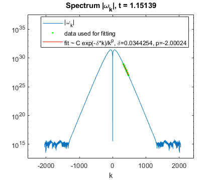
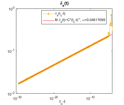
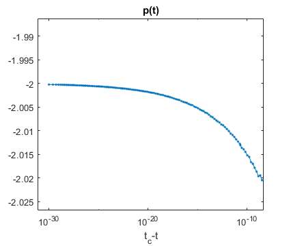
Figure 3: Left panel: The Fourier spectrum $|\hat{\omega}_{k}|$ at a particular time $t=1.15139$ from the same simulation as in Fig. 2 with $a=2/3$. The red line represents a fit to the model (62) with green line showing the portion of the $|\hat{\omega}_{k}|$ used for the least-squares fit. Center and right panels: time dependence of $\delta_{x}(t)=\tanh{\left(\frac{\delta(t)}{2}\right)}$ and $p(t)$ recovered from the fit of the spectrum to Eq. (62) at different times. The red solid line at the center panel represents a fit to the model $\delta_{x}(t)\sim(t_{c}-t)^{\alpha}.$

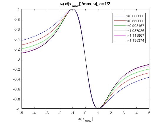
Figure 4: Convergence of time-dependent numerical solution of Eqs. (54)-(55) with $a=1/2$ (left panel) and $a=2/3$ (right panel) to the self-similar solution (6). In both cases we used IC1 (58). Solutions shrink horizontally and increase in amplitude vertically until collapse occurs at $t=t_{c}$, $t_{c}\approx 1.180602237542$ (left panel) and $t_{c}\approx 1.272876000077$ (right panel). Solutions are plotted in $x$-space, where $x=\tan(\frac{q}{2})$. Horizontal and vertical scales are dynamically changed in both panels to exactly match the positions and amplitudes of the local maximum at $x=x_{max}$ and minimum at $x=-x_{max}$.

Figure 5: Convergence of the time-dependent numerical solution of Eqs. (54)-(55) to the self-similar profile (6) as $t\rightarrow t_{c}$. Here $a=2/3$ and we use the generic initial condition $\omega_{0}(x)=-\frac{1}{64}\left(\frac{1}{(x-x_{1}^{+})^{3}}+\frac{1}{(x-x_{1}^{-})^{3}}\right)-\frac{\mathrm{i}}{3}\left(\frac{1}{(x-x_{2}^{+})^{2}}-\frac{1}{(x-x_{2}^{-})^{2}}\right)+\frac{1}{32}\left(\frac{1}{(x-x_{3}^{+})^{3}}+\frac{1}{(x-x_{3}^{-})^{3}}\right)+\frac{\mathrm{i}}{96}\left(\frac{1}{(x-x_{4}^{+})^{2}}-\frac{1}{(x-x_{4}^{-})^{2}}\right),$ where $x_{1}^{\pm}=-1\pm\frac{\mathrm{i}}{4},x_{2}^{\pm}=-\frac{1}{2}\pm\frac{\mathrm{i}}{2},x_{3}^{\pm}=1\pm\frac{\mathrm{i}}{4},x_{4}^{\pm}=\frac{3}{2}\pm\frac{\mathrm{i}}{8}.$ The solution is shown at two different moments in time, where for each time we overlaid the self-similar profile as in Fig. 4, matching their corresponding maximum and minimum positions horizontally and vertically.

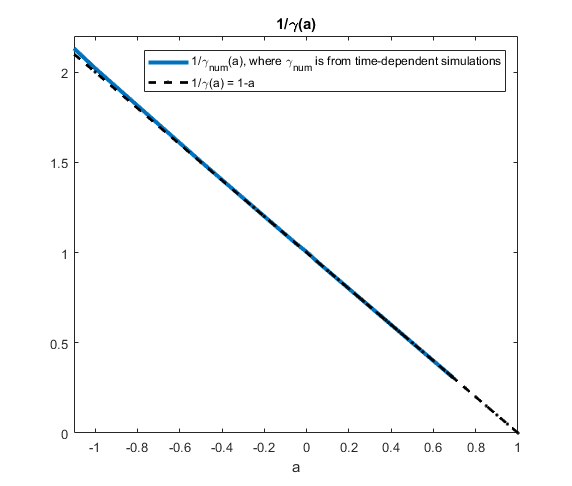
Figure 6: Dependence of $\gamma_{num}(a)=1-p(a)$ using $p(a)$ obtained via time-dependent simulations by the fit to Eq. (62). These data are also provided in Table 1. Also shown is $\gamma(a)=\frac{1}{1-a}$ from Eq. (21) for comparison. Here we plot $1/\gamma(a)$ instead of $\gamma(a)$ for the easier comparison.

For $0\leq a<a_{c}$ (with $a_{c}$ given by Eq. (8)) and for both IC1 (58) and IC2 (59), we find that $\delta_{x}(t)$ evolves in time toward 0 while $p(t)$ approaches a constant value after a quick transient phase, see Fig. 3 (right panel). We observe spontaneous formation of a universal self-similar solution profile of the form (6) during time evolution (see Fig. 4). These self-similar profiles, as well as the value of $\alpha$ in $\delta_{x}(t)$ and the terminal value of $p(t)$ as $t\rightarrow{t_{c}}$ are the same for a wide class of ICs (e.g. one can change a power of singularity in IC2 from $-2$ to any negative number below $-2$ and/or change numerical values of both $V_{c}>0$ and $T_{c}>0$). Thus, these self-similar profiles are only functions of the parameter $a$. Table 1 provides the universal values of $\alpha$ and $p$ vs $a$. Fig. 1 shows the dependence of $\alpha(a)$ on $a$. However, one can also find particular IC in which finite time singularities do not form. Two such choices are -IC1 and -IC2, i.e. IC1 (58) and IC2 (59) taken with the opposite sign. In these two cases we did not observe collapse or singularity formation in finite time, but rather an algebraic-in-time approach of a singularity to the real line, $\delta_{x}(t)\sim 1/t^{\mu},\mu>0$. Other smooth generic initial conditions that were tried were found to produce blow up after an initial transient, as exemplified in Fig. 5. These transients made the simulation considerably slower (due to the need for more modes in the spectrum of to resolve the solution down to double precision round-off). However, in a space-time neighborhood of the singularity these solutions recover the same self-similar profile as shown in Fig. 4, see also Fig. 5. We note that the velocity $u(x,t)$ evolves toward the self-similar profile (48) with $\max\limits_{x}|u|\to\infty$ for $0<a<a_{c}$. Below we focus on IC1 and IC2, but the reader should but keep in mind that they appear generic.

Table 1: Table of values of $\alpha$, $p$ and $\alpha_{2}$ extracted via fits to $\delta_{x}(t)$, $|\hat{\omega}_{k}|$ and $\max|\omega_{x}(x,t)|$ in time-dependent simulations of Eqs. (54)-(55) for various values of $a$. Also shown are values of $\alpha_{e}$ and $\beta$ obtained from eigenvalue problem simulations of Eqs. (67) and (55) described in Section 9. Accuracy of $\alpha(a)$ (for $-1\leq a\leq 0.689$) and $\alpha_{2}(a)$ (for $-1\leq a\leq 0.689066533$) is at least 3-4 digits of precision, whereas accuracy of $\alpha_{e}(a)$ is about 3-4 digits of precision for $a<0.3$ and at least 5 digits of precision for $a\geq 0.3$, with more precision for $0.3\leq a\leq 0.6890665$.

$a$	$\alpha_{e}$	$\beta$	$p$	$\alpha$	$\alpha_{2}$
-5	-	-	0.855	7.495	7.517
-2	-	-	0.680	3.444	3.422
-1	-	-	0.505	2.208	2.206
-0.5	-	-	0.335120	1.603747	1.600222
-0.25	1.296593455	-	0.200942	1.303708	1.302424
-0.2	1.239824952	-	0.167139	1.243558	1.242436
-0.15	1.181358555	0.133308	0.130811	1.183300	1.182701
-0.1	1.121312899	0.100401	0.091110	1.122630	1.122093
-0.05	1.061051829	0.060633	0.047696	1.061617	1.061334
0	1	0	0.004	1.000243	1.000019
0.05	0.938365701	-0.070205	-0.052759	0.938381	0.938288
0.1	0.876129662	-0.136336	-0.111326	0.876329	0.876309
0.15	0.813179991	-0.240380	-0.176727	0.813219	0.813215
0.2	0.749369952	-0.338799	-0.250265	0.749519	0.749549
0.25	0.684513621	-0.460507	-0.333582	0.684650	0.684671
0.265	0.664818990	-0.500444	-0.360765	0.664827	0.664830
0.3	0.618374677	-0.610349	-0.428762	0.618375	0.618377
0.35	0.550648498	-0.787978	-0.538583	0.550661	0.550655
0.4	0.480939257	-0.939823	-0.666732	0.4809431	0.4809429
0.425	0.445184823	-0.97452	-0.739156	0.4451863	0.4451860
0.4375	0.427049782	-0.993899	-0.777804	0.4270512	0.4270508
0.45	0.408728507	-1	-0.818193	0.40872820	0.40872838
0.5	0.333333333	-1	-1.0000007	0.33333354	0.33333340
0.55	0.253852136994	-1	-1.222218	0.25385226	0.25385213
0.6	0.169098936470	-1	-1.4999991	0.16909915	0.1690989367
0.65	0.077532635626630	-1	-1.857141	0.07753269	0.07753263562662
2/3	0.045170944220367	-1	-1.999997	0.04517096	0.04517094422035
0.68	0.018526534283004	-1	-2.125013	0.01852675	0.01852653428270
0.685	0.008351682345844	-1	-2.175083	0.00835210	0.008351682345843
0.689	0.000137203824593	-1	-2.219165	0.00013724	0.000137203824603
0.68905	3.409705703117e-05	-1	-2.221589	3.4145e-05	3.4097057039e-05
0.68906	1.347443362884e-05	-1	-2.220924	1.3418e-05	1.3474433654e-05
0.689066	1.10065641e-06	-1	-2.221505	1.0808e-06	1.1006564176e-06
0.6890665	6.950143e-08	-1	-2.223142	-	6.9501438524e-08
0.68906653	7.632094e-09	-1	-2.222128	-	7.6321058379e-09
0.689066533	1.445152e-09	-1	-2.220519	-	1.4451679770e-09
0.6890665335	4.13992e-10	-1	-2.205923	-	4.1401557848e-10
0.6890665337	1.537e-12	-1	-2.220897	-	1.5519e-12
0.6890665337007	9.43093e-14	-1	-2.227272	-	1.1097e-13
0.68906653370074	1.18169e-14	-1	-2.222533	-	2.7574e-14
0.689066533700745	1.505397e-15	-1	-2.221208	-	1.4711e-14
0.6890665337007457	6.169686e-17	-1	-	-	-
0.7	-	-	-	-	-0.02281
0.75	-	-	-	-	-0.13435
0.8	-	-	-	-	-0.26008
0.85	-	-	-	-	-0.40384
0.9	-	-	-	-	-0.57118
0.95	-	-	-	-	-0.76643
1	-	-	-	-	-1.000000056

Using the terminal values of $p$ extracted by fits to Eq. (62) with various $a$, and employing Eq. (63) to recover $\gamma$ from $p$, we confirmed the formula $\gamma(a)=\frac{1}{1-a}$ (see Theorem 1 and Eq. (21) in Section 2) and the corresponding formula $p(a)=\frac{-a}{1-a}$ within 0.5% for $0\leq a<a_{c}$. Fig. 6 shows the numerical approximation, $\gamma_{num}(a)=1-p(a)$ using values of $p(a)$ from Table 1 as well as the theoretical value $\gamma=\frac{1}{1-a}$ for comparison. We note that the plot of $1/\gamma_{num}(a)$ in Fig. 6 stops at $a=a_{c}$, since it is difficult to obtain accurate values of $p(a)$ (and hence $\gamma_{num}(a)$) from time-dependent simulations when $a>a_{c}$. This is due to a transition that occurs at $a=a_{c}$, in which the fitted singularity for $a<a_{c}$ corresponding to collapse is no longer closest to the real-$x$ line when $a>a_{c}$.

In addition to Fourier fitting, we also extract values of $\alpha$ in an alternative way (these values are called $\alpha_{2}$ below), using the spatial derivative of the self-similar solution (6) given by

$$\omega_{x}(x,t)=\frac{1}{(t_{c}-t)^{1+\alpha}}f^{\prime}\left(\frac{x}{(t_{c}-t)^{\alpha}}\right).$$ (64)

Using Eq. (64) we fit $\max\limits_{x}|\omega_{x}(x,t)|$ to the model $\max\limits_{x}|\omega_{x}(x,t)|\propto\frac{1}{(t_{c}-t)^{1+\alpha_{2}}}$ to find $\alpha_{2}.$ Values of $\alpha_{2}$ for various $a$ are also gathered in Table 1 for comparison with values of $\alpha$. We confirmed that $\alpha$ and $\alpha_{2}$ obtained using the above two methods for $0<a\lesssim 0.689$ agree within a relative error of $<0.02\%$.

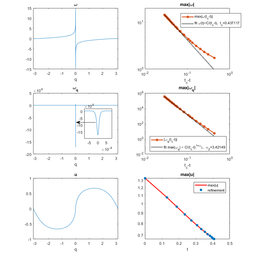
Figure 7: Results from simulations of Eqs. (54)-(55) with $a=-2$ and initial condition IC2 (60). Left panels: the solution $\omega(q,t)$, its derivative $\omega_{q}(q,t)$, and $u(q,t)$ for $t=0.407228$. Right panels: Time dependence of the maximum values of these functions. Dashed lines show the prediction of Eq. (6) with $\alpha_{2}$ extracted from simulations as explained in the text.

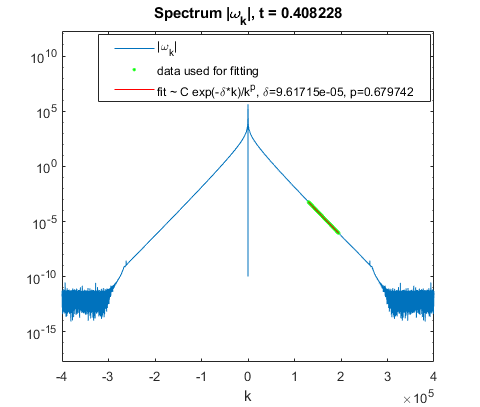
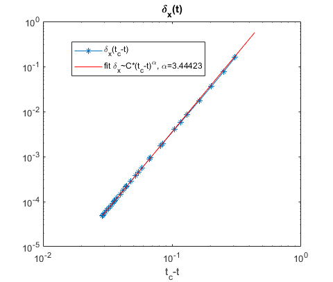
Figure 8: Left panel: The Fourier spectrum $|\hat{\omega}_{k}|$ at time $t=0.407228$ from the same simulation as in Fig. 7. The red line represents a fit to the model (62) with green line showing portion of the $|\hat{\omega}_{k}|$ used for the fit. Center and right panels: Time dependence of $\delta_{x}(t)=\tanh{\left(\frac{\delta(t)}{2}\right)}$ and $p(t)$ recovered from fit of the spectrum to Eq. (62) at different times. The red solid line at the center panel represents a fit to the model $\delta_{x}(t)\propto(t_{c}-t)^{\alpha}.$

For $a<0$ we observe a similar finite time blow up starting from both IC1 and IC2 with $\max\limits_{x}|\omega|\rightarrow{\infty}$ as $t\rightarrow{t_{c}}$ according to the self-similar profile in Eq. (6). The extracted values of $\alpha$, $p$ and $\alpha_{2}$ for $a<0$ are also given in Table 1, see also Figs. 7 and 8 for results of simulations with $a=-2$ and IC2. The velocity $u(x,t)$ during the temporal evolution approaches the self-similar profile (48) near the singularity location at $x=q=0$. A qualitative difference for $a<0$ (in comparison with $0<a<a_{c}$) is that the self-similar profile (48) approaches zero because $\alpha>1$ in the former case, while away from the spatial singularity location the value of $u(x,t)$ is generally nonzero, even at $t\to t_{c}.$ This extends the result of CastroCordoba , who proved that there is finite-time singularity formation for $a<0$ in the case of odd compactly supported data $\omega(x,0)\in C_{c}^{\infty}(\mathbb{R})$ with ${\mathcal{H}}\omega(0,0)>0$, to examples with analytic initial data.

We obtained much more accurate values of $\alpha(a)$ (up to 14 digits of precision) by numerically solving the nonlinear eigenvalue problem, Eq. (47), for a self-similar solution of Eq. (1) (see Section 9). In contrast, for $a_{c}$ we were able to obtain 14 digits of accuracy using both time-dependent simulations and the nonlinear eigenvalue problem with double precision arithmetic. Another 3 digits of precision are obtained (for a total of 17 digits of precision) if quadruple precision arithmetic is used in the nonlinear eigenvalue problem.

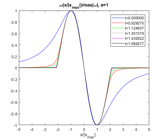
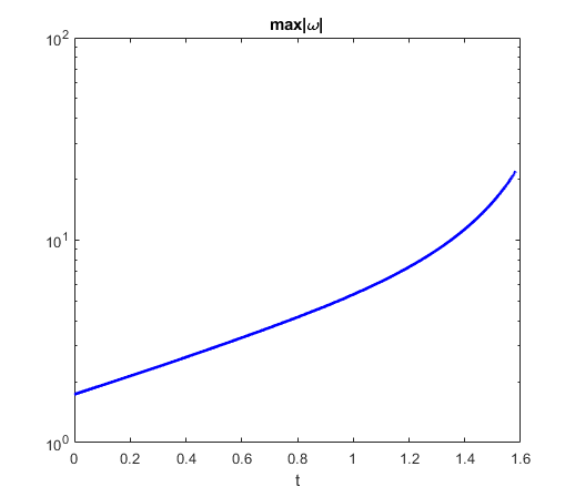
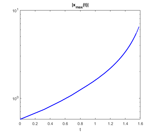
Figure 9: Left panel: Convergence of the time-dependent numerical solution to Eqs. (54)-(55) with $a=1$ and IC2 (60) to a self-similar profile with compact support. The solution expands horizontally and stretches vertically until blowing up at $t=t_{c}\approx 1.77864$. The solution is plotted in $x$-space, where $x=\tan(\frac{q}{2})$, and is scaled both horizontally and vertically to exactly match the positions of the local maximum and minimum. Center and right panels: The time dependencies of $\max\limits_{x}|\omega(x,t)|$ and the absolute value its location $x_{max}(t)$ on $t$.

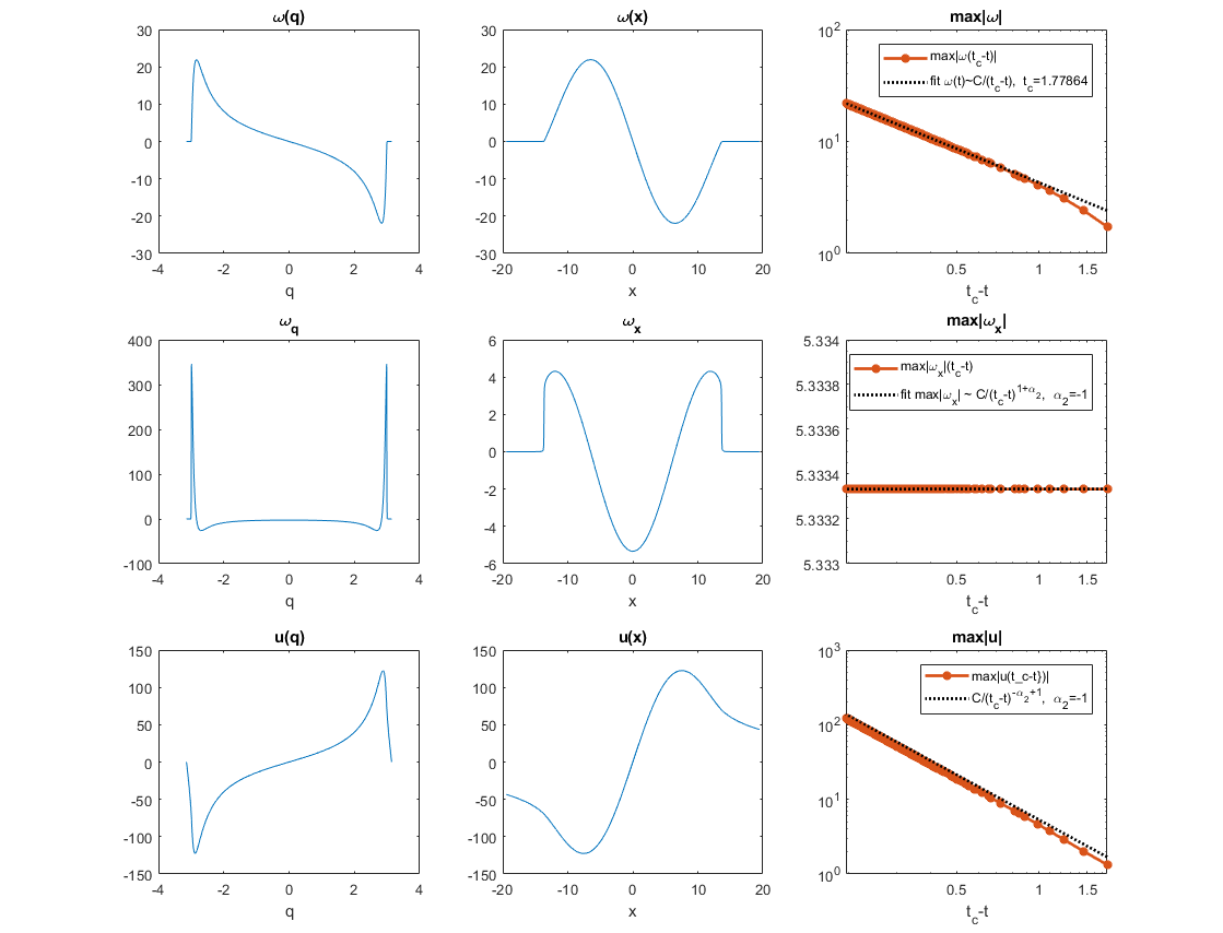
Figure 10: Results of the same simulation as in Fig. 9 with $a=1$ showing solution $\omega(q,t)$, $\omega_{q}(q,t)$ and $u(q,t)$ in $q$-space (left panels) as well as the same solution in $x$-space (center panels) at time $t=1.582477.$ Right panels show the time dependence of their maximum values as functions of $(t_{c}-t)$, where $t_{c}$ is the blow-up time extracted from the fit to $\max|\omega(x,t)|\propto\frac{1}{(t_{c}-t)}$.

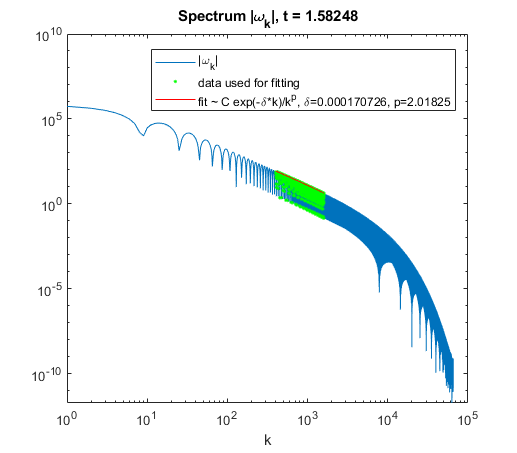
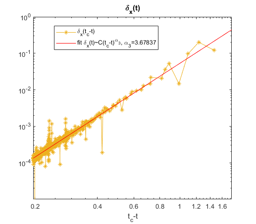
Figure 11: Left panel: The Fourier spectrum $|\hat{\omega}_{k}|$ at time $t=1.58248$ from the same simulation as in Fig. 10 with $a=1$. The red line represents a fit to the model (62) with green line showing a portion of the $|\hat{\omega}_{k}|$ used for the fit. Right panel: Time dependence of $\delta_{x}(t)=\tanh{\left(\frac{\delta(t)}{2}\right)}$ recovered from the fit of the spectrum to Eq. (62). The red solid line in the right panel represents a fit to the model $\delta_{x}(t)\propto(t_{c}-t)^{\alpha_{3}}.$

We have also performed simulations specifically with $a=1$ since this special case was addressed in Chen et al. ChenHouHuang , who proved for this value of $a$ the existence of an “expanding” self-similar solution of the type (6) for the problem on $x\in\mathbb{R}$. In this case $f(\xi)$ is an odd function with a finite support and $\alpha=-1$. Their solution implies that $\omega(x,t)\to f^{\prime}(0)x$ as $t\to t_{c}$ for any finite value of $x\in\mathbb{R}$ while the boundary of the compact support expands infinitely fast into large $|x|$ as $t\to t_{c}.$ Our numerical findings show an approach to this kind of expanding solution with compact support starting from a generic analytic initial condition, see Figs. 9 and 10. This verifies that the similarity solution is attracting. The solution grows in amplitude and expands faster than exponentially in time, which is demonstrated by semi-log plots of $\max\limits_{x}|\omega(x)|(t)$ and its location $x_{max}(t)$ in the middle and right panels of Fig. 9. It obeys the self-similar profile (6) and forms a finite time singularity at $t=t_{c}$. Fig. 10 (right panels) confirms the scales $\max\limits_{x}|\omega(x)|\propto 1/(t_{c}-t)$ and $|\omega_{x}(x=0)|\propto 1/(t_{c}-t)^{1+\alpha}=const$ with $\alpha=-1$. One can also see (from the middle panel of Fig. 10) that $\max\limits_{x}|\omega_{xx}(x)|\to\infty$ as $t\to t_{c}$. We are able to simulate the growth in amplitude of $\omega(x)$ only by about one order of magnitude with our spectral code, since the spectrum widens very quickly as $t\rightarrow{t_{c}}$ and decays slowly, i.e., $|\hat{\omega}_{k}(x)|\sim k^{-2}$, as seen in Fig.11 (left panel). The approach to a self-similar solution with compact support is expressed in the complex $x$-plane by the approach of complex singularities (identified as branch points from our simulations) located at $x=x_{sing}$ to the real line near the boundaries of compact support. The small distances $|Im(x_{sing})|$ of these singularities to the real line for $t$ near $t_{c}$ means that the solution is “almost of compact support” with “almost a jump” in the first derivative at the boundary of “compact support” in $x$-space. The singularity locations scale like

$$x_{sing}\simeq\pm(t_{c}-t)^{\alpha}x_{b}\pm\mathrm{i}\,(t_{c}-t)^{\alpha_{3}}y_{b}$$ (65)

(i.e. there are four symmetrically located singularities), where $\alpha=-1$ and $\alpha_{3}\approx 3.68.$ Here the real constants $t_{c}$, $x_{b}$ and $y_{b}$ depend on the IC. Note that $\alpha_{3}$ is different from $\alpha$ because it characterizes the approach of the solution to the compactly supported profile (6). In contrast, the value $\alpha=-1$ is fully determined by Eq. (6) and characterizes the self-similar behaviour of the central part of the solution. The nonzero value of $\alpha_{3}$ suggests that the “almost compactly supported” solution turns into a truly compactly supported solution at $t=t_{c}$, with a jump in the first derivative. Due to oscillations in the spectrum, it is difficult to accurately extract the value of $\alpha_{3}$ from the fit to $\delta_{x}(t)\sim(t_{c}-t)^{\alpha_{3}}$. However, using rational approximation via the AAA algorithm (see details about AAA in Section 10) we can observe two pairs of branch cuts with branch points approach the real line near $x=\pm(t_{c}-t)^{\alpha}x_{b}$ as $t\rightarrow{t_{c}}$, similar to the case $a=0.8$. One can see from Fig. 12 (right panel) that the structure of the singularity for $a=0.8$ is similar to the $a=1$ case.

For $a_{c}<a<1$ and both IC1 or IC2, we similary observe finite time singularity formation with an expanding self-similar solution approaching a compactly supported profile (described again by Eq. (6)). This is qualitatively similar to the $a=1$ case, but involves different values of $\alpha$. Another difference compared to the $a=1$ case is that there is a discontinuity in a higher-order derivative at the boundary of ”compact support”, instead of a jump in the first derivative $\omega_{x}$ as occurs for $a=1$. Figs. 12 - 14 show the results of simulations with the parameter $a=0.8$ and IC2 (60). Here we find a jump in $\omega_{xx}$ forming at the boundary of “compact support”. Fig. 13 (right) shows the growth of both $\max\limits_{x}|\omega(x)|$ and $\max\limits_{x}|\omega_{x}(x)|=|\omega_{x}(x=0)|$ as functions of $t_{c}-t$ confirming the scales $\max\limits_{x}|\omega(x)|\sim 1/(t_{c}-t)$ and $|\omega_{x}(x=0)|\sim 1/(t_{c}-t)^{1+\alpha}$ with $\alpha=-0.26008$.

Qualitatively similar to the case $a=1$, for $a_{c}<a<1$ we again observe two pairs of branch cuts approach the real line as $t\rightarrow{t_{c}}$ according to Eq. (65). For example, when $a=0.8$ we find that $\alpha=-0.26008$ and $\alpha_{3}\approx 0.908$, see Fig. 12 (right panel). It was challenging to accurately extract values of $\delta(t)$ and $p(t)$ from a fit to Eq. (62) due to the spectrum being oscillatory, see the left panel of Fig. 14. The right panel of Fig. 14 provides the best fit which we were able to obtain for $\delta(t)$. The fitting parameter $p(t)$ was more sensitive to the oscillations and did not appear to stabilize at any particular value, so we do not provide a plot for it here.

This type of oscillation in the spectrum occurs when there are two symmetric singularities that are equally close to the real line. In this case, a more elaborate fitting procedure with additional parameters to account for the oscillation can yield improved results, see e.g. Ref. BakerCaflischSiegelJFM1993 . However, such fits are also more delicate to implement, and are beyond the scope of the current work.

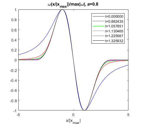
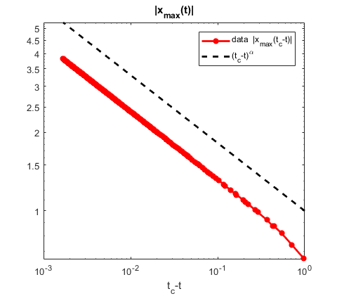
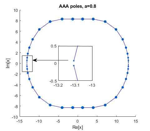
Figure 12: Left panel: Convergence of time dependent numerical solution to Eqs. (54)-(55) with $a=0.8$ and IC2 (60) to a self-similar profile with compact support. The solution expands horizontally and stretches vertically until blowing up at $t=t_{c}\approx 1.32761$. The solution is plotted in $x$-space, where $x=\tan(\frac{q}{2})$, and is scaled both horizontally and vertically to exactly match the positions of the local maximum and minimum. Center panel: The time dependence $x_{max}(t)$ of the location of $\max\limits_{x}\omega(x)$. The dashed lines shows that it scales like $x_{max}(t)\propto(t_{c}-t)^{\alpha}$ with $\alpha\simeq-0.26008$ as $t\rightarrow{t_{c}}$. Right panel: The structure of complex singularities at $t=1.32593$ obtained using AAA-algorithm (described in Section 10) that approximates the solution by a set of simple poles, $\omega(x)\approx\omega_{AAA}(x)=\sum_{i=1}^{m-1}\frac{a_{i}}{x-b_{i}}$. The simple poles are shown as dots at locations $b_{i}$ with a size of dot scaled with $\log_{10}|a_{i}|$. The branch cuts are shown as lines connecting the dots, and form ‘U-shaped’ curves in the upper and lower complex plane. The accumulation of poles approximates two pairs of branch points near the real line. The location of these branch points scale as $x_{sing}\sim\pm(t_{c}-t)^{\alpha}x_{b}\pm\mathrm{i}y_{0}(t_{c}-t)^{\alpha_{3}}y_{b}$, where $x_{0},y_{0}>0$, $\alpha=-0.26008$ and $\alpha_{3}\approx 0.908$.

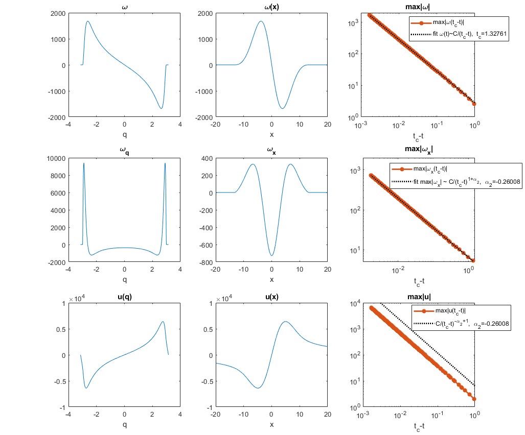
Figure 13: Results of the same simulation as in Fig. 12 with $a=0.8$ showing $\omega(q,t)$, $\omega_{q}(q,t)$, and $u(q,t)$ in $q$-space (left panels) as well as in $x$-space (center panels) at time $t=1.32593.$ Right panels show the time dependence of their maximum values as functions of $(t_{c}-t)$, where $t_{c}$ is the blow-up time extracted from the fit to $\max|\omega(x,t)|\propto\frac{1}{(t_{c}-t)}$.

Figure 14: Left panel: The Fourier spectrum $|\hat{\omega}_{k}|$ at a particular time $t=1.32593$ from the same simulation as in Fig. 12 with $a=0.8$. The red line represents a fit to the model (62) with the green line showing the portion of the $|\hat{\omega}_{k}|$ used for the fit. The purple line shows a fit to the rougher model (62) with $\delta=0$. Right panel: Time dependence of $\delta_{x}(t)=\tanh{\left(\frac{\delta(t)}{2}\right)}$ recovered from the fit of the spectrum to Eq. (62). The red solid line at the right panel represents a fit to the model $\delta_{x}(t)\propto(t_{c}-t)^{\alpha_{3}}.$

Simulations with ICs either of type -IC1 or -IC2 and $a_{c}<a\leq 1$ resulted in monotonically decaying $\max\limits_{x}|\omega(x,t)|$ and $\max\limits_{x}|u(x,t)|.$ The maximum slope $\max\limits_{x}|\omega_{x}(t)|=|\omega_{x}(x=0,t)|$ is found to approach a constant value for $a=1$ while it decays for $a<1.$ Also, $\max\limits_{x}|\omega_{xx}(x,t)|$ grows algebraically as a function of $t$, while $\delta_{x}(t)$ decays algebraically, $\delta_{x}(t)\sim 1/t^{\mu},\mu>0$. Since these ICs do not result in a finite-time singularity formation, we do not discuss these cases in further detail.

For $a\gtrsim 1.3$ and for both IC1 and IC2, we observe global existence of the solution. The vorticity $\omega$ has the form an an expanding self-similar function which approaches a compactly supported profile (in the scaled variable $\xi$) with infinite slope at the boundary of the compact region, so that $\max\limits_{x}|\omega|\rightarrow{0}$ and $\max\limits_{x}|\omega_{x}|,\max\limits_{x}|u|\rightarrow{\infty}$ as $t\rightarrow{\infty}$ (although $\omega_{x}(x=0)\rightarrow{0}$ as $t\rightarrow{\infty}$). The complex singularities approach the real line in infinite time with positions that scale like $x_{sing}=\pm x_{0}\exp{(\kappa_{1}t^{\nu_{1}})}\pm\mathrm{i}y_{0}\exp{(-\kappa_{2}t^{\nu_{2}})}$, where the constants $\kappa_{1},\kappa_{2},\nu_{1},\nu_{2}>0$ depend on $a$. For both -IC1 and -IC2 we again observe global existence of the solution with decay of $\omega$ and infinite growth of $\omega_{x}(x=0)$, with an infinite slope forming at $x=0$ and a singularity approaching the real line like $x_{sing}=0\pm\mathrm{i}y_{0}\exp{(-\kappa_{2}t^{\nu_{2}})}$, where $y_{0},\kappa_{2},\nu_{2}>0.$

For $1<a\lesssim 1.3,$ we find from simulations that initially $\max\limits_{x}|\omega|$ grows. This period of initial growth is long, with the spectrum widening so quickly that it was challenging to distinguish between a finite time singularity and global existence when $a$ is near 1, but we have numerical evidence of global existence for $a$ at least as small as 1.3, as described in the previous paragraph.

Here we summarize the behaviour of solutions to Eqs. (54)-(55) on $x\in\mathbb{R}$, and its dependence on the parameter $a$, for quite generic smooth IC:

• $a<a_{c}$ with $\alpha(a)>0$: Collapse in $\omega,$ i.e. $\max\limits_{x}|\omega|\to\infty$ at the finite time $t_{c}.$ As $t\to t_{c}$, solutions with generic IC approach the shrinking universal self-similar profile (6) near the spatial location of $\max\limits_{x}|\omega|$. As $t\to t_{c},$ the profiles shrink to zero width. The self-similar solution has leading order complex singularities in agreement with Theorem 1 and Eq. (21). The location of these singularities approaches the real line as $x_{sing}=x_{0}\pm\mathrm{i}\,\delta_{x}(t)$, where $\delta_{x}(t)\propto(t_{c}-t)^{\alpha}$, $\alpha=\alpha(a)>0$. In particular, $x_{0}=0$ for both IC1 or IC2. Also $u(x,t)$ near $x_{0}$ follows the self-similar profile (48) with $\max\limits_{x}|u|\to\infty$ for $0<a<a_{c}$.

• $a_{c}<a\leq 1$ with $\alpha(a)<0$: Blow up in both $\omega$ and $u$ at the finite time $t_{c}.$ As $t\to t_{c}$, solutions with generic IC approach the expanding self-similar profile Eq. (6) which has compact support. As $t\to t_{c}$, the rate of expansion turns infinite. The complex singularities closest to the real line correspond to the boundaries of compact support, and they approach the real line as $x_{sing}\sim\pm(t_{c}-t)^{\alpha}x_{b}\pm\mathrm{i}\,(t_{c}-t)^{\alpha_{3}}y_{b}$, where $\alpha=\alpha(a)<0$ and $\alpha_{3}(a)>0$,

• $a\gtrsim 1.3:$ global existence of solutions with $\max\limits_{x}|\omega|\rightarrow{0}$, $\max\limits_{x}|\omega_{x}|,\max\limits_{x}|u|\rightarrow{\infty}$ and $\omega_{x}(x=0)\rightarrow{0}$ as $t\rightarrow{\infty}$. The complex singularities approach the real line exponentially in time as $x_{sing}=\pm x_{0}\exp{(\kappa_{1}t^{\nu_{1}})}\pm\mathrm{i}y_{0}\exp{(-\kappa_{2}t^{\nu_{2}})}$, where $\kappa_{1},\kappa_{2},\nu_{1},\nu_{2}>0$.

9 Numerical solution of nonlinear eigenvalue problem on the real line

Similar to the transformation of Eq. (1) to Eqs. (54)-(55) in Section 7, we obtain a transformed equation for self-similar solutions of Eq. (47) by mapping the interval $(-\pi,\pi)$ of the auxiliary variable $q$ onto the real line $(-\infty,\infty)$ as

$$\xi=\tan\left(\frac{q}{2}\right).$$ (66)

With this mapping Eq. (47) turns into

$$\begin{split}&{\mathcal{M}}f:=f+\alpha\sin{q}\,f_{q}=-a(1+\cos{q})gf_{q}+f[{\mathcal{H}}^{2\pi}f+C_{f}^{2\pi}]:={\mathcal{N}}[f]f,\quad q\in[-\pi,\pi],\\ &(1+\cos{q})g_{q}={\mathcal{H}}^{2\pi}f+C_{f}^{2\pi},\end{split}$$ (67)

where the $2\pi$-periodic Hilbert transform ${\mathcal{H}}^{2\pi}$ and the constant $C_{f}^{2\pi}$ are defined in Eqs. (55), (56), and the linear operator $\mathcal{M}$ is now defined in $q$ space by the l.h.s. of the first Eq. in (67). We also define in equation (67) the quadratically nonlinear operator $\mathcal{N}[f]$ such that ${\mathcal{N}}[f]f$ represents the r.h.s. of the first Eq. in (67) with $g$ expressed through the second equation in (67) as

$$g=\partial_{q}^{-1}\left[\frac{{\mathcal{H}}^{2\pi}f+C_{f}^{2\pi}}{(1+\cos{q})}\right],\quad\partial_{q}^{-1}p:=\int\limits_{-\pi}^{q}p(q^{\prime})dq^{\prime}.$$ (68)

Then Eq. (67) takes the following operator form

$${\mathcal{M}}f={\mathcal{N}}[f]f.$$ (69)

A linearization of Eq. (69) about $f$ together with Eqs. (67) and (68) result in

$${\mathcal{L}}[f]\delta f:=-{\mathcal{M}}\delta f-a(1+\cos{q})\partial_{q}^{-1}\left[\frac{{\mathcal{H}}^{2\pi}\delta f+C_{\delta f}^{2\pi}}{(1+\cos{q})}\right]f_{q}$$

$$-a(1+\cos{q})\partial_{q}^{-1}\left[\frac{{\mathcal{H}}^{2\pi}f+C_{f}^{2\pi}}{(1+\cos{q})}\right]\delta f_{q}$$

$$+\delta f[{\mathcal{H}}^{2\pi}f+C_{f}^{2\pi}]+f[{\mathcal{H}}^{2\pi}\delta f+C_{\delta f}^{2\pi}],$$ (70)

where ${\mathcal{L}}[f]$ is the linearization operator and $\delta f$ is the deviation from $f.$

Taking $\delta f=f$ in Eq. (9) and using Eqs. (67), (69) to express the nonlinear terms in $f$ through the linear terms proves the following theorem:

Theorem 4. The solution $f$ of Eq. (67) satisfies the relation

$${\mathcal{L}}[f]f={\mathcal{M}}f.$$ (71)

Corollary 1. The invertability of the operator $\mathcal{M}$ (see Section 6) and Eq. (71) imply that the operator ${\mathcal{\ }M}^{-1}{\mathcal{L}}[f]$ has the eigenvalue $\lambda=1$ with eigenfunction $f$, which is the same as the solution $f$ of Eq. (67).

Similar to Eq. (57), we approximate a solution of Eq. (67) as a truncated Fourier series

$$f(q)=\sum_{k=-N}^{k=N-1}{\hat{f}_{k}e^{\mathrm{i}kq}}.$$ (72)

Then the discrete Fourier transform allows us to rewrite Eq. (67) in matrix form as

$${\bf M}\,{\hat{\bf f}}=\widehat{{\mathcal{N}}[f]f},\quad{\bf M}:=\begin{pmatrix}1&-\frac{\alpha k_{2}}{2}&&&\\ \frac{\alpha k_{1}}{2}&1&-\frac{\alpha k_{3}}{2}&&\\ &\frac{\alpha k_{2}}{2}&1&\dots&\\ &&\dots&\dots&-\frac{\alpha k_{2N}}{2}\\ &&&\frac{\alpha k_{2N-1}}{2}&1\\ \end{pmatrix},$$ (73)

where ${\hat{\bf f}}=(\hat{f}_{k_{1}},\hat{f}_{k_{2}},\ldots,\hat{f}_{k_{2N}})^{T}$ is a column vector, the tridiagonal matrix ${\bf M}\in\mathbb{R}^{2N\times 2N}$ represents the Fourier transform of the operator $\mathcal{M}$ and $\widehat{{\mathcal{N}}[f]f}$ is the column vector of Fourier coefficients of ${{\mathcal{N}}[f]f}$. Also $k_{1}:=-N,\,k_{2}:=-N+1,\ldots,\,k_{2N}:=N-1.$ Note that the tridiagonal form of ${\bf M}$ is a consequence of the term $\sin(q)=\frac{e^{\mathrm{i}q}-e^{-\mathrm{i}q}}{2\mathrm{i}}$in the definition of $\mathcal{M}$ in Eq. (67).

We solve Eq. (71) in the truncated Fourier representation (73) by iteration using the generalized Petviashvili method (GPM) LY2007 which relates the $n+1$th iteration $\hat{\bf f}^{n+1}$ to the $n$th iteration $\hat{\bf f}^{n}$ of $\hat{\bf f}$ as follows

$$\hat{\bf f}^{n+1}-\hat{\bf f}^{n}=\left([-\hat{\bf f}^{n}+{\bf M}^{-1}\widehat{{\mathcal{N}}[f]f^{n}}]-\left(1+\frac{1}{\Delta\tau}\right)\frac{\langle\hat{\bf f}^{n},-{\bf M}\,{\hat{\bf f}}^{n}+\widehat{{\mathcal{N}}[f]f^{n}}\rangle}{\langle\hat{\bf f}^{n},{\bf M}\,{\hat{\bf f}}^{n}\rangle}\hat{\bf f}^{n}\right)\Delta\tau,$$ (74)

where superscripts give the iteration number, $\langle{\bf a}\,,\,{\bf b}\rangle:=\sum_{k=-N}^{k=N-1}\bar{a}_{k}b_{k}$ is the complex dot product and $\Delta\tau$ is a parameter that controls the convergence rate of the iterations. At each iteration we need to solve Eq. (73) for $\hat{\bf f}$ (assuming $\widehat{{\mathcal{N}}[f]f}$ is given) to effectively compute ${\bf M}^{-1}\widehat{{\mathcal{N}}[f]f^{n}}$. Since ${\bf M}$ is a tridiagonal matrix, this is easily done in $O(N)$ numerical operations in Fourier space. We note that if one tries to avoid the FFT and iterate Eq. (67) directly in $q$ space, then the corresponding matrix $M$ on the l.h.s. of Eq. (67) would be a full matrix and each iteration would require $O(N^{2})$ numerical operations.

A fixed point of the iteration (74) corresponds to the solution of Eq. (71). The straightforward iteration of (71) (instead of (74)) would diverge because of the positive eigenvalue $\lambda=1$ of Corollary 1 for the linearized operator ${\mathcal{\ }M}^{-1}{\mathcal{L}}[f]$. In contrast, Eq. (71) ensures an approximate projection into the subspace orthogonal to the corresponding unstable eigenvector $f.$ The original Petviashvili method Petviashvili1976 is the nonlinear version of Eq. (74) for the particular value $\Delta\tau=1$ and is often successful with both partial differential equations (PDEs) (see e.g. Refs. LY2007 ; YangBook2010 ) and nonlocal PDEs (see e.g. Ref. LushnikovOL2001 ). However, the linear operator ${\mathcal{\ }M}^{-1}{\mathcal{L}}[f]$ generally has extra eigenvalues preventing the convergence of the original Petviashvili method. GPM however uses the freedom in choice of the parameter $\Delta\tau$ to achieve convergence even with such extra eigenvalues, see Refs. DyachenkoLushnikovKorotkevichJETPLett2014 ; LY2007 ; YangBook2010 for more discussion.

An additional complication that arises in our Eq. (67), compared with the straightforward use of GPM in general PDEs, is that we do not know $\alpha$ in advance. Instead, for each value of $a$ there is a nonlinear eigenvalue $\alpha(a)$ to Eq. (67) that we need to determine. If we use a general value of $\alpha$, then the iteration (74) would not converge because the solution of Eq. (67) does not exist for such general values of $\alpha.$

To address this additional complication, we make an initial guess of $\alpha=\alpha_{guess}$ for fixed $a$ and iterate Eq. (67) for $\alpha_{guess}$. If $\alpha_{guess}<\alpha(a)$ then the generalized Petviashvili iteration (after an initial transient) shrinks towards $q=0$. If $\alpha_{guess}>\alpha(a)$ then the solution expands away from $q=0$. We used the bisection method to determine $\alpha(a)$ for a given $a$. We start from a large enough interval $[\alpha_{L},\alpha_{R}]$, so that $\alpha(a)\in[\alpha_{L},\alpha_{R}]$. Then we try $\alpha_{guess}=(\alpha_{L}+\alpha_{R})/2$ and based on the shrinking vs. expanding of iterations for $\alpha_{guess},$ we obtain the updated values $[\alpha_{L},\alpha_{R}]$. These updated values ensure a factor 2 decrease of the length of the updated interval $[\alpha_{L},\alpha_{R}]$, completing the first step of the bisection method. We continue such bisection steps until convergence to $\alpha(a)$ (i.e., until the residual of Eq. (67) decreases down to near round-off values and does not decrease anymore). For each updated $\alpha_{guess}$ we use the solution from the previous bisection step to speed-up the convergence. We judged the expansion/shrinking of the solution by tracking the movement of its maximum point which was determined as a critical point of the function $f^{\prime}(q)=\sum_{k=-N}^{k=N-1}{\mathrm{i}k\hat{f}_{k}e^{\mathrm{i}kq}}$ using spectral interpolation and a root-finding algorithm. Also, in order to pass over the initial transient dynamics (that depends on the initial guess of the solution) we skip $10/\Delta\tau-20/\Delta\tau$ initial GPM iterations before judging the expansion/shrinking of the solution to classify the current $\alpha_{guess}$. The larger $\Delta\tau$ we used, the less iterations were needed, but too large a $\Delta\tau$ leads to instability of the algorithm, so we need to keep it under a certain level. For the initial guess of the solution we typically used IC2 from Eq. (59) with $V_{c}=1/2$ for $0.6<a<a_{c}$, and $N=64;$ $\Delta\tau$ was reduced from $0.1$ at $a=0.6$ to $10^{-4}$ near $a_{c}.$ For $a<0.6$ we used $\Delta\tau=0.1-1$ and progressively smaller $V_{c}$ (down to $2^{-14}$) and larger $N$ (up to $2^{22}$) because of the slowly decaying tails of the function $f(q)$ for small $a$ (see the next paragraph). Fig. 15 illustrates the convergence of the $[\alpha_{L},\alpha_{R}]$ interval to $\alpha(a)$ and convergence of the residual of Eq. (67) with bisection iterations for $a=0.2$, starting with an initial condition IC2 in (59) with $V_{c}=1/2^{12}\approx 2.44\times 10^{-4}$ (singularity is at $\xi=\mathrm{i}Vc$) and $N=2^{18}$. The converged solution is shown in Fig. 16 (left panel) with a closest singularity at a distance $\xi_{c}=7.43\cdot 10^{-5}$ from the real line in $\xi$-space and at a distance $q_{c}=1.49\cdot 10^{-4}$ in $q$-space.

Figure 15: Convergence of the interval $[\alpha_{L},\alpha_{R}]$ to $\alpha(a)$ (left panel) and convergence of the residual of Eq. (73) (right panel) for the iteration (74) with $a=0.2.$ Here we used IC2 (59) with $V_{c}=2^{-12}\approx 2.44\cdot 10^{-4}$ and $N=2^{18}$ as the zeroth iteration.

We note that the symmetry (51) implies that $\xi_{c}$ can be stretched by an arbitrary positive constant. The iteration (74) generally converges to different values of $\xi_{c}$ depending on IC (i.e., the zeroth iteration). After that one can rescale any such solution in $\xi$ by any fixed value of $\xi_{c}.$ This rescaling freedom can also be seen through the existence of the free parameter $\tilde{v}_{c}$ in the exact solutions (3) and (38), (39).

We computed self-similar profiles $f(\xi)$ and $g(\xi)$ for various values of $a<a_{c}$ to obtain $\alpha(a)$ shown in Table 1 as $\alpha_{e}(a).$ Additionally, we make sure that the $f(\xi)$ profile tails scale as in Eq. (49) at $\xi\to\pm\infty$ and we also fit the $g(\xi)$ profile tails to the power law

$$g(\xi)\propto\xi^{\beta}.$$ (75)

Fig. 17 show examples of such scaling and fit for $a=0.2$. Several other curves with different powers of $\xi$ are present on the graphs for comparison. The fitted values of $\beta(a)$ are given in Table 1 and Fig. 16 (right panel). Ignoring for the moment the Hilbert transform, the integration operator $\partial_{\xi}^{-1}$ involved in determining $g(\xi)$ from $f(\xi)$ in Eq. (47) suggests that

$$g(\xi)\propto\xi^{-\frac{1}{\alpha}+1}\ \text{at}\ \xi\to\pm\infty,$$ (76)

which implies that

$$\beta=-\frac{1}{\alpha}+1.$$ (77)

However, the Hilbert transform in Eq. (47) can affect this scaling. We find that (77) is valid for $0<a\lesssim 0.4$, while a transition to the constant scaling $\beta=-1$ occurs around $a\approx 0.45$ as seen in Table 1 and Fig. 16 (right panel). In particular, the exact analytical solution (34) for $a=1/2$ and $\alpha=1/3$ implies that $\beta=-1$ which is consistent with Table 1 and Fig. 16 (right panel). One can see from comparison of Eqs. (33) and (34) that the Hilbert transform indeed prevents the naive scaling (76) in this particular case. In contrast, the scaling (49) follows from the linear operator $\mathcal{M}$ as discussed in Section 6. That scaling was confirmed with high precision in our simulations so we do not show it in Table 1. For $a<0$ we find that $g(\xi)$ has two regions with two different scalings, see Fig. 18 for $a=-0.1$. While the tail of $g(\xi)$ still decays as $\xi\to\pm\infty$, there is an intermediate scaling regime which approximately obeys (77) as seen in Fig. 18 (left panel). We are able to observe this intermediate scaling for $-0.2\leq a<0$. Going below $a=-0.2$ is difficult for the GPM method as the tails of $f(\xi)$ and $g(\xi)$ decay very slowly and it requires more than $10^{6}$ grid points to achieve good accuracy. For $a<0$ the values of $\beta$ in Table 1 and in Fig. 16 (right panel) are from this intermediate scaling.

Figure 16: Left panel: $a=0.2$. Functions $f(\xi)$ and scaled $g(\xi)$ obtained by the iteration (74). Right panel: Power-law of scaling of the tails of $g(\xi)$ vs. $a$.

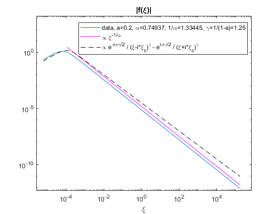
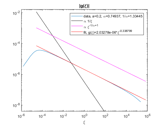
Figure 17: $a=0.2$. Left panel: Tail of $f(\xi)$ from Fig. 16 (left panel). The dashed line shows the decay of $f(\xi)$ when it is approximated by its leading order singularities alone, as obtained from (17), neglecting the l.s.t. Right panel: Tail of $g(\xi)$ from Fig. 16 (left panel) compared with different power laws.

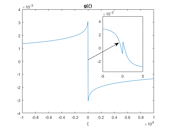
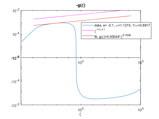
Figure 18: Plots of $g(\xi)$ for $a=-0.1$. Left panel: Graph of $g(\xi)$ showing two extrema (one maximum and one minimum) in each half-space of $\xi$. The inset gives a magnified view showing extrema at small $\xi$. Right panel: Log-log plot of $g(\xi)$ for positive $\xi$. Here $g(\xi_{0})=0$ at $\xi_{0}\approx 0.41$. Solid lines show the scaling (76) and a fit to power law (75).

We estimate that our iteration procedure provides at least 5-8 digits of precision of in $\alpha(a)$ and 2-3 digits of precision in $\beta(a)$ for $a\geq 0.3$, when the spectrum of $f(q)$ is fully resolved. The values of $\alpha(a)$ and $\beta(a)$ were challenging to obtain with more than 3-4 and $\sim$2 digits of accuracy, respectively, for $a\lesssim 0.2$ (corresponding to $\alpha\gtrsim 0.75$) and especially for $a<0$ ($\alpha>1$) since we could not resolve the Fourier spectrum $|\hat{f}_{k}|$ down to round-off level $10^{-16}$, even with $N=2^{22}$ modes. At its root, this is due to the slow decay of $f(\xi)\sim|\xi|^{-1/\alpha}$ for $|\xi|\rightarrow\infty$ and relatively large $\alpha$.

The numerical values of $\beta$ in the scaling (75) are important to distinguish between solutions with infinite and finite energy $E_{K}$ (10), which as mentioned is of interest in analogy with the question of singularity formation in the 3D Euler and Navier-Stokes equations. Assuming that the solution is close to the self-similar profile (6), changing the variable from $x$ to $\xi$ in (10) and using the self-similar profile (48) of the velocity $u(x,t)$ we obtain that

$$E_{K}=E_{K}^{selfsim}+E_{K}^{rest},$$ (78)

where

$$E_{K}^{selfsim}=\int\limits^{x_{b}}_{-x_{b}}u^{2}(x)\mbox{d}x\sim\tau^{3\alpha-2}\int\limits^{\xi_{b}}_{-\xi_{b}}g^{2}(\xi)\mbox{d}\xi,\ \xi_{b}=\frac{x_{b}}{\tau^{\alpha}},$$ (79)

is the kinetic energy of the approximately self-similar part of the solution located at $x\in[-x_{b},x_{b}]$ and $E_{K}^{rest}$ is the kinetic energy of the numerical solution outside of this interval. Here we define the cutoff value $x=x_{b}$ as the spatial location where the numerical solution deviates from the self-similar profile (6) by $5\%$, while inside of the interval $[-x_{b},x_{b}]$ the relative deviation is less than $5\%$. We determine the variable $\xi$ by the same type of procedure as in Fig. 4. Then $x_{b}$ is determined by $5\%$ criterion above. We find from simulations with $a<a_{c}$ that

$$x_{b}(t)\approx const\sim\tau^{0}.$$ (80)

Such behaviour is typical for collapsing self-similar solutions, see e.g. Ref. SulemSulem1999 ; KuznetsovZakharov2007 ; DyachenkoLushnikovVladimirovaKellerSegelNonlinearity2013 ; LushnikovDyachenkoVladimirovaNLSloglogPRA2013 . It implies that $\xi_{b}\to\infty$ as $t\to t_{c}$.

There is no qualitative difference between integrals $I_{g,\xi_{b}}:=\int\limits^{\xi_{b}}_{-\xi_{b}}g^{2}(\xi)\mbox{d}\xi$ and $I_{g,\infty}=\int\limits^{\infty}_{-\infty}g^{2}(\xi)\mbox{d}\xi$ provided $I_{g,\infty}<\infty$. The finiteness of $I_{g,\infty}$ requires that $\beta<-\frac{1}{2}$ for the scaling of the tails of $g(\xi)$ in (75). Using equation (77) we obtain that $\beta=-\frac{1}{2}$ implies $\alpha=\frac{2}{3}$, i.e. $\beta<-\frac{1}{2}$ for $\alpha<\frac{2}{3}$. From the interpolation of the data of Table 1 we find that $\alpha=\frac{2}{3}$ corresponds to $a=0.265\pm 0.001$. Therefore for a self-similar profile, $I_{g,\infty}<\infty$ for $a>0.265\pm 0.001$ and $I_{g,\infty}=\infty$ for $a<0.265\pm 0.001$.

However, we have to take into account that $I_{g,\xi_{b}}$ is multiplied by $\tau^{3\alpha-2}$ in equation (79). This means that in the limit $t\to t_{c}$ and for $\alpha<\frac{2}{3}$, there is a competition between the decrease of $\tau^{3\alpha-2}$ and the growth of $I_{g,\xi_{b}}$ as $\xi_{b}\to\infty.$ The scaling (77) for Eq. (75) is valid for $a\lesssim 0.4$ as seen in Fig. 16 (right panel). It implies that $I_{g,\xi_{b}}\propto\xi_{b}^{2\beta+1}=\tau^{-\alpha(2\beta+1)}x_{b}^{2\beta+1}$ for $a<0.265\pm 0.001$ and $t\to t_{c}.$ Then using Eqs. (77), (79) and (80) we obtain that $E_{K}^{selfsim}\sim\tau^{0}\sim const$. Also since the main dynamics is happening in $x\in[-x_{b},x_{b}]$ with $x_{b}(t)\sim const,$ we conclude that $E_{K}^{rest}\to const$ as $t\to t_{c}$, so overall the growth of $E_{K}(t)$ as $t\to t_{c}$ is very slow (i.e., slower than any power of $\tau$) for such $a$ where the scaling (77) is true. This result is in excellent agreement with our direct calculation of $E_{K}(t)$ from time-dependent simulations which shows that for $a<0.265\pm 0.001$ the kinetic energy grows more slowly than $\log(\tau)$ or any power of $\tau$ as $t\to t_{c}$; see Fig. 19 (left panel) for $a=0.2$.

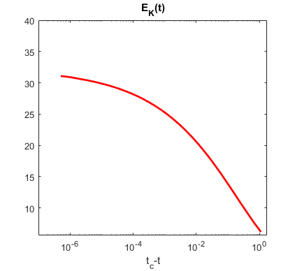
Figure 19: Growth of the kinetic energy $E_{K}$ over time. Left panel: $a=0.2$, semi-log plot of $E_{K}$ vs. $\tau=t_{c}-t$ shows that $E_{K}$ grows slower than $\log(\tau)$ or any power of $\tau$ as $t\to t_{c}$. Center panel: $a=0.4$, verification of the scaling $E_{K}\sim\tau^{3\alpha-2}$ in (79) with $I_{g,\infty}<\infty$. Right panel: $a=1.5$, $E_{K}\to\infty$ exponentially as $t\to\infty$.

For $0.265\pm 0.001<a\leq 1$ the kinetic energy $E_{K}\to\infty$ as $t\to t_{c}$ (while being finite for any $t<t_{c}$), since $\alpha<0$ and $E_{K}\sim\tau^{3\alpha-2}\to\infty$ as $t\to t_{c}$ with $I_{g,\infty}<\infty$; see Fig. 19 (center panel) for a verification of this scaling when $a=0.4$. For $a\gtrsim 1.3$, which corresponds to an expanding solution with infinite time singularity, $E_{K}\to\infty$ as $t\to\infty$, while being finite for any $t<\infty$; see Fig. 19 (right panel) for an example with $a=1.5$. For $a>a_{c}$, the above splitting of $E_{K}$ into two parts is no longer valid but we nevertheless verify the claims above via time-dependent numerical simulation.

For some values of $a$ we computed $\alpha(a)$ and nonlinear self-similar profiles with much higher precision. For example, we used 68-digit arithmetic (using commercially available Advanpix MATLAB Tolbox https://www.advanpix.com) for $a=2/3$ to find that
$\alpha(a)=0.0451709442203672185156916552716968964156893201125622408995729\ldots$ and to compute $f(q)$ up to $\sim$60 digits of precision, see Fig. 20. High precision computations help validate the results from double precision calculations, and allow us to obtain a good quality analytic continuation of the solution $f(\xi)=f(q(\xi))$ from the real line $\xi\in\mathbb{R}$ to the complex plane $\xi\in\mathbb{C}$ via the AAA-algorithm TrefethenAAA , see Section 10 below.

10 Analytical continuation into the complex plane by rational approximation and structure of singularities

Fits of the Fourier spectrum using Eq. (62) allows us to find only the singularity closest to the real line. A more powerful numerical technique of analytical continuation based on rational interpolants AGH2000 ; DyachenkoLushnikovKorotkevichPartIStudApplMath2016 ; DyachenkoDyachenkoLushnikovZakharovJFM2019 ; TrefethenAAA allows us to go deeper (further away from the real line) into the complex plane, well beyond the closest singularity. However, analytic continuation further from the real line often requires an increase in numerical precision, even well above the standard double precision DyachenkoLushnikovKorotkevichPartIStudApplMath2016 ; DyachenkoDyachenkoLushnikovZakharovJFM2019 . In this paper we use a rational interpolation based on a modified version of the AAA algorithm of Ref. TrefethenAAA . AAA finds an approximation $f_{AAA}(\xi)$ to a complex function $f(\xi)$ in barycentric form by minimizing the $L_{2}$ error of the approximation on the real line.

The barycentric form is given by

$$f_{AAA}(\xi):=\frac{n(\xi)}{d(\xi)}=\frac{\sum_{i=1}^{m}\frac{w_{i}f_{i}}{\xi-\xi_{i}}}{\sum_{i=1}^{m}\frac{w_{i}}{\xi-\xi_{i}}},$$ (81)

where $m\geq 1$ is an integer, $\xi_{i}$ are a set of real distinct support points, $f_{i}$ are a set of real data values, and $w_{i}$ are a set of real weights determined by $L_{2}$ error minimization. The integer $m$ is increased until the $L_{2}$ error between $f_{AAA}(\xi)$ and $f(\xi)$ on the real line is on the level of $10^{-PR}$, where $PR$ is the current working precision. For analytic functions the error decreases exponentially in $m$.

The Barycentric form (81) is a quotient of two polynomials $n(\xi)$ and $d(\xi)$. A partial fraction expansion of this quotient results in a sum of $m-1$ first order complex poles, $f_{AAA}^{poles}(\xi)=\sum_{i=1}^{m-1}\frac{a_{i}}{\xi-b_{i}}$, with locations $b_{i}$ and residues $a_{i}$ determined by the values of $w_{i}$ and $\xi_{i}$. The pole locations $b_{i}$, which are zeros of $d(\xi)$, are determined by solving a generalized eigenvalue problem described in Ref. TrefethenAAA . The values of the residues $a_{i}$ can be computed using L’Hospital’s rule $a_{i}=res(f_{AAA},b_{i})=n(b_{i})/d^{\prime}(b_{i})$. If our data for an analytic function is given with precision $PR$ on the real line, AAA and subsequent computations of $b_{i}$ approximate the location of single poles with maximum precision $\sim PR$, double poles with precision $\sim PR/2$, and triple poles with precision $\sim PR/3$, etc. The progressive loss of precision in higher order poles is due to cancellation errors. We find we can achieve the reduced error $|f(\xi)-f_{AAA}^{poles}(\xi)|\approx 10^{-PR}$ on the real line in the case of higher order poles if we increase the precision of intermediate computations in the generalized eigenvalue problem by a factor of two for double poles and a factor of three for triple poles. We additionally modified the original AAA algorithm TrefethenAAA to deal with odd and even functions more efficiently and output more symmetrical sets of poles.

Figure 20: Convergence of the residual (left panel) and spectrum of the solution (right panel) to Eq. (73), computed with $a=2/3$ and 68-digit precision, and using IC2 (59) with $V_{c}=1/16=0.0625$ and $N=2048$ in the zeroth iteration.

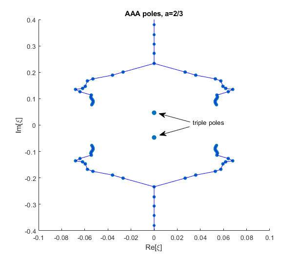
Figure 21: The structure of the complex singularities of the solution from Fig. 20 approximated by a set of simple poles, $f(\xi)\approx f_{AAA}^{poles}(\xi)=\sum_{i=1}^{m-1}\frac{a_{i}}{\xi-b_{i}}$ using the AAA algorithm (left panel), and the relative error on the real line between the solution $f(\xi)$ and its approximation $f_{AAA}(\xi)$ (right panel). The simple poles are shown as dots at locations $b_{i}$ with the size of dot scaled with $\log_{10}|a_{i}|$. The branch cuts are approximated as lines connecting the dots. The triple poles locations are $\xi\approx\pm\mathrm{i}0.04678$ and branch points are located at $\xi=\xi_{branch}\approx\pm 0.05398\pm\mathrm{i}0.07674$.

In the particular case $a=2/3,$ we use 68-digit precision arithemetic for the numerical solution of $f(\xi)$ described at the end of Section 9, and incorporate this into the AAA algorithm. This method shows that the closest singularities to the real line are a pair of the third order poles $\propto 1/(\xi\pm\mathrm{i}\chi_{c})^{3}$, in full agreement with Theorem 1 (Eq. (21) of Section 2) and the Fourier spectrum analysis of Section 8. The location $\xi=\pm\mathrm{i}\chi_{c}$ (here $Re(\chi_{c})>0$ and $Re(\chi_{c})\gg|Im(\chi_{c})|$) and the third order type of these poles are automatically approximated by the AAA algorithm as three simple poles $\sum_{i=1}^{3}\frac{a_{i}}{\xi-b_{i}}$ lying very close to each other ($|b_{1}-b_{2}|,|b_{2}-b_{3}|<1.54\cdot 10^{-12})$ with the sum of their residues being essentially zero ($|\sum_{i=1}^{3}{a_{i}}|/|a_{1}|\approx 4.64\cdot 10^{-47}$). We define the location of the triple pole by the average $\mathrm{i}\chi_{c}=\sum_{i=1}^{3}{b_{i}}/3$ and have verified that the dipole moment defined by $D:=\sum_{i=1}^{3}{(b_{i}-\mathrm{i}\chi_{c})a_{i}}$ is negligible, $|D|\approx 1.2\cdot 10^{-29}$. In contrast, the quadrupole moment $Q:=\sum_{i=1}^{3}{(b_{i}-\mathrm{i}\chi_{c})^{2}a_{i}}$ is distinct from zero, $|Q|\approx 1.5\cdot 10^{-4}$, so this multipole is well approximated by $\frac{Q}{(\xi-\mathrm{i}\chi_{c})^{3}}.$ The complex conjugate point $\xi=-\mathrm{i}\chi_{c}$ was treated in a similar way, i.e., by another set of 3 poles of AAA.

We find that the rest of the singularities of $f(\xi)$ are branch points with branch cuts extending from them. AAA approximates branch cuts by sets of poles, and Refs. DyachenkoLushnikovKorotkevichPartIStudApplMath2016 ; DyachenkoDyachenkoLushnikovZakharovJFM2019 demonstrate how to recover branch cuts from this set of poles by increasing the numerical precision. The increase of numerical precision requires an increase in the number of poles $m$ in rational interpolants to match the precision. These poles, which are located on a branch cut, become more dense with the increase in precision and thus recover the location of the branch cut in the continuous (infinite precision) limit. The main motivation for using 68-digit precision in this paper was to ensure that we robustly recover branch cuts, see Fig. 21 (left panel). In the particular case $a=2/3,$ double precision allows us to robustly see $\sim 30$ poles, whereas 68-digit precision allows us to see $\sim 150$ poles. The number of poles we use for a fixed precision is determined by the minimal number of AAA poles to match the numerical precision of the solution on the real line. Increasing the number poles beyond this minimal number produces spurious poles with very small residues, which is the analog of the round-off floor in the Fourier spectrum. We note that the exact shape of the branch cuts is not fixed analytically – the AAA algorithm simply provides a set of poles that corresponds to the smallest $L_{2}$ error on the real axis for the given number of poles. Thus, the AAA approximation of the branch cut might move with a change of the precision. In contrast, the branch points computed by the algorithm are fixed. One can see 4 branch points in Fig. 21 (left panel), with two branch cuts going upward and coalescing on the imaginary axis and extending further to $+\mathrm{i}\infty.$ Another two branch cuts extend downwards and merge on the imaginary axis before going off to $-\mathrm{i}\infty$.

Our investigations of complex singularities via AAA approximations show that for any $a$, except for $a=\frac{n-1}{n},\quad n=1,2,3,\dots$ (which corresponds to the integer values $\gamma=n$ in Eq. (21)), there is another pair of vertical branch cuts coming out of $\xi=\pm\mathrm{i}\chi_{c}$ and coalescing with the rest of the branch cuts on the imaginary axis. For $a<a_{c}$ the side branch points are always above the main singularity at $\xi=\pm\mathrm{i}\chi_{c}$ and their locations are $\xi_{branch}=\pm\epsilon_{1}(a)\chi_{c}\pm\mathrm{i}(1+\epsilon_{2}(a))\chi_{c},\,$ where roughly $\epsilon_{1}(a)\sim 1,\,\epsilon_{2}(a)\sim 1$. In particular, $Re[\xi_{branch}]/\chi_{c}<0.74$, $Im[\xi_{branch}]/\chi_{c}>2$ for $a<0.6$; $Re[\xi_{branch}]/\chi_{c}\approx 1.15$, $Im[\xi_{branch}]/\chi_{c}\approx 1.64$ for $a=2/3$ and $Re[\xi_{branch}]/\chi_{c}\approx 1.23$, $Im[\xi_{branch}]/\chi_{c}\approx 1.51$ near $a=a_{c}$.

11 Results of time dependent simulations and Petviashvili iterations for periodic BC

Motivated by simulations of the generalized CLM equation (1) in Ref. Okamoto2008 for $2\pi$-periodic BC with $a=1$, we performed simulations for a wide range of values of the parameter $a.$ For this we used the periodic version of the Hilbert transform ${\mathcal{H}}^{2\pi}$ (55) in Eq. (1) instead of ${\mathcal{H}}$.

Simulations for $a<a_{c}$ show collapsing solutions with $\alpha>0$, and different types of IC give qualitatively similar results near the collapse time $t=t_{c}$ as in the real line $x\in\mathbb{R}$ case with the same $\alpha(a)$ (see Table 1). Hence we do not describe them here. Expanding solutions for $a>a_{c}$ behave differently since the finite spatial interval $[-\pi,\pi]$ arrested the increasing width of the solution at large enough times. Thus we focus our discussion on $a>a_{c}$ and present detailed results of our simulations, in particular the cases of $a=0.8$ and $a=1$.

We performed a simulation with $a=0.8$ and initial condition

$$\omega_{0}(x)=-\frac{4}{3}[\sin(x)+0.5\sin(2x)]$$ (82)

which is qualitatively similar to the particular case (60) of IC2 (59), with $q$ replaced by $x$ and $V_{c}=1,T_{c}=1$. After an initial spatial expansion, the solution is arrested by the periodic boundary conditions. This arrest results in the qualitative change of the dynamics, see for example the right panel of Fig. 22 for the time dependence of the location $x_{max}(t)$ of $\max\limits_{x}|\omega(x)|.$ At later times we still find a finite time blow up of the solution with $\max\limits_{x}|\omega(x)|$ and $\max\limits_{x}|u(x)|\rightarrow{\infty}$ as $t\rightarrow{t_{c}}$. However, instead of Eq. (6), the solution converges to a new universal self-similar blow-up profile given by Eq. (9), as demonstrated in left panel of Fig. 22. A comparison of Eqs. (6) and (9) reveals that we can formally obtain Eq. (9) by setting $\alpha=0$ in Eq. (6) (although Eq. (9) has periodic boundary conditions, vs. decaying BC of Eq. (6)). We note that taking the limit $a\rightarrow{a_{c}^{-}}$ in Eq. (6), we also obtain $\alpha=0.$ However, it remains unknown if Eq. (9) can be obtained from the continuation of Eq. (6) across $a=a_{c}$.

The spectrum $\hat{\omega}_{k}$ is initially exponentially decaying but expands and becomes mostly algebraically decaying (similar to Fig. 14). Finite precision arithmetic only “sees” algebraic decay $|\hat{\omega}_{k}(x)|\sim k^{-3}$ when $t$ is close enough to $t_{c}$, see Fig. 24. This is because of a jump in $\omega_{xx}$ forming at $x=\pm\pi$, see Fig. 23 (left and middle panels). Due to the spectrum being initially oscillatory it was difficult to accurately extract values of $\delta(t)$ and $p(t)$ from a fit to Eq. (62), but using a nonoscillatory spectrum which emerges later in the simulation we were able to recover some data for $\delta(t)$ and $p(t)$ as shown in Fig. 24. There, one can see that $\delta(t)\rightarrow{0}$ and $p(t)\rightarrow{3}$ as $t\rightarrow{t_{c}}$.

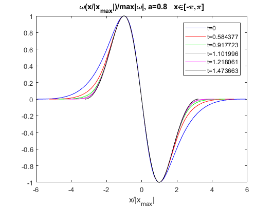
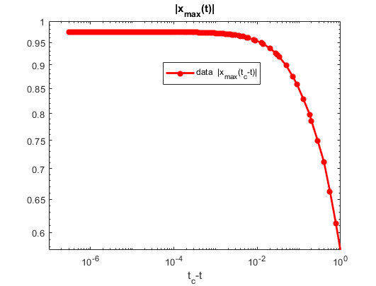
Figure 22: Left panel: Convergence of time-dependent numerical solution of Eqs. (1) and (55) with $a=0.8$ and IC (82) to a universal self-similar profile. The solution expands horizontally (until arrested by the boundary condition) and extends vertically, blowing up at $t=t_{c}=1.4736630\ldots.$ The plot is scaled vertically by $\max\limits_{x}|\omega|$ and horizontally by the location $x_{max}(t)$ of $\max\limits_{x}|\omega|$. Right panel: Time dependence of $|x_{max}(t)|$, which shows slowdown and eventual arrest of the horizontal expansion of the solution.

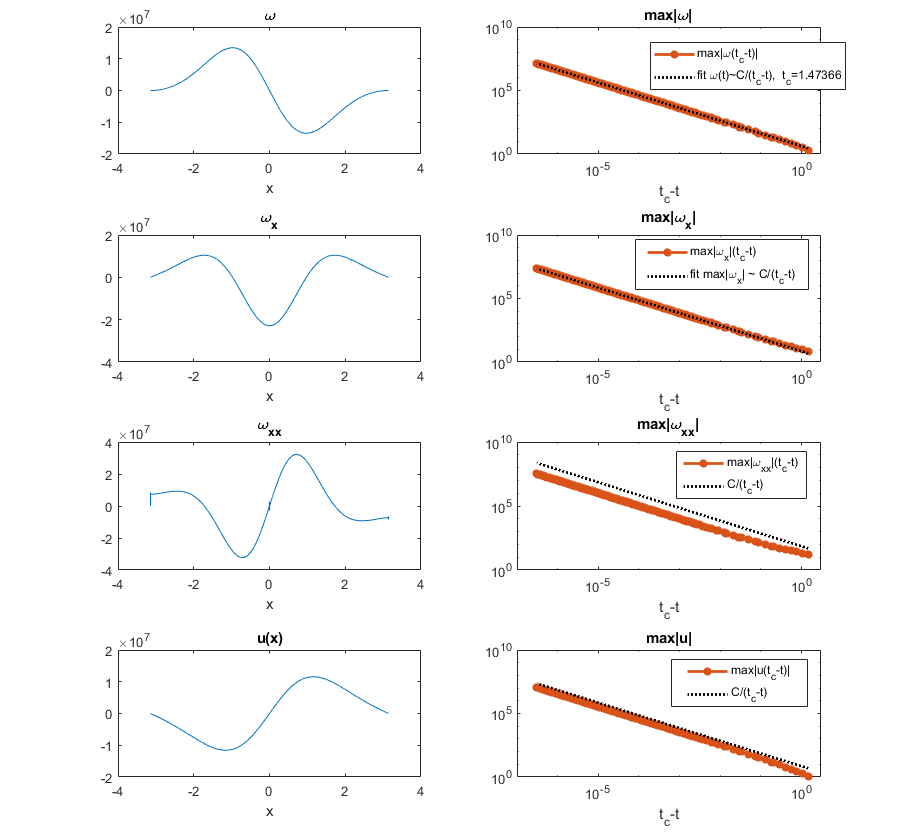
Figure 23: Results of the simulation of Eqs. (1) and (55) with $a=0.8$ and IC (82). Left panels: $\omega(x,t)$, its derivatives $\omega_{x}(x,t)$, $\omega_{xx}(x,t)$, and $u(x,t)$ at $t=1.4736627.$ Right panels: the growth of maximum values of the corresponding quantities over time.

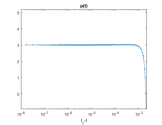
Figure 24: Left panel: Log-log plot of the Fourier spectrum $|\hat{\omega}_{k}|$ from Fig. 23 at $t=1.4736627$ and $a=0.8$. The red line represents a fit to the model (62) with green line showing a portion of the $|\hat{\omega}_{k}|$ used for the fit. Center and right panels: $\delta(t)$ and $p(t)$ obtained from the fit of $|\hat{\omega}_{k}|$ to Eq. (62) at different times. Red lines in the center panel also show a fit to the model $\delta(t)\propto(t_{c}-t)^{\alpha_{3}}$.

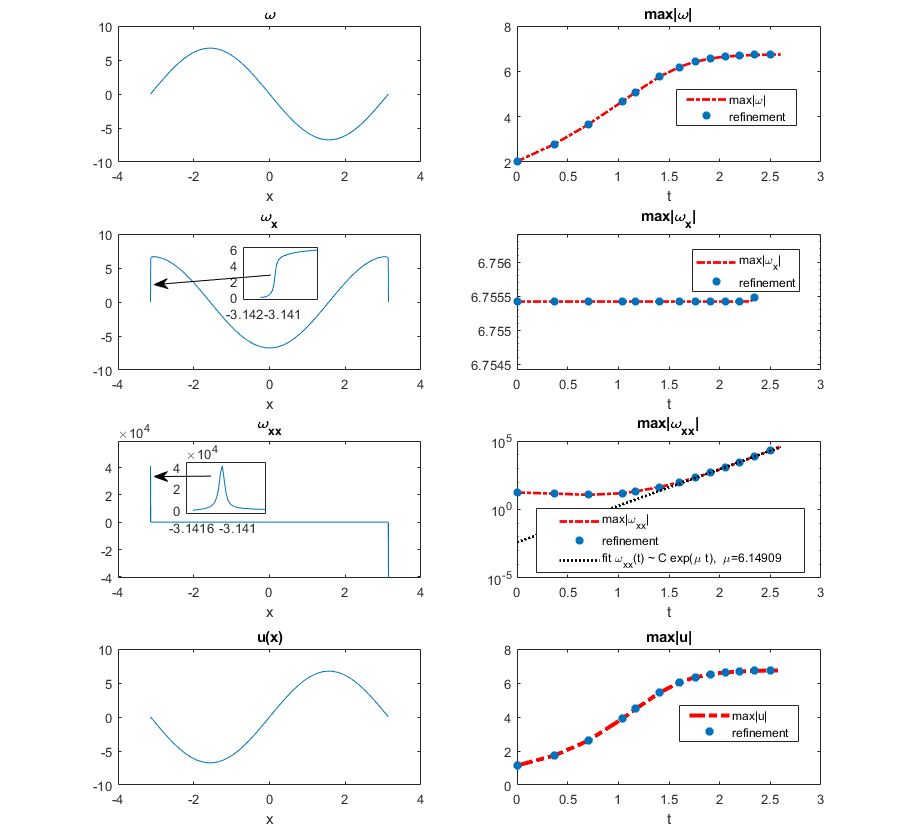
Figure 25: Results of the simulation of Eqs. (1) and (55) with $a=1$ and IC (82) showing $\omega(x,t)$, its derivatives $\omega_{x}(x,t)$, $\omega_{xx}(x,t)$, and $u(x,t)$ at $t=2.60205$. Also shown is the growth of their maximum values as functions of time.

For $a=1$ we considered two different types of ICs. The first one is IC (82), for which we observe global existence of the solution. Initially the amplitude of the solution $\omega(x)$ grows in time, similar to the infinite domain case. But this growth slows down at later times and eventually reaches a plateau with the the same behaviour in $u(x)$, see Fig. 25. Also $\max\limits_{x}|\omega_{x}|=|\omega_{x}(x=0)|$ remains nearly constant throughout the simulation. We observe unbounded growth of $|\omega_{xx}|$ near $x=\pm\pi$ that appears to be exponential in time. Due to the spectrum being oscillatory it was difficult to accurately extract values of $\delta(t)$ and $p(t)$ from a fit to Eq. (62). However, using AAA rational approximation we were able to observe two pairs of branch cuts approach the real line near $x=\pm\pi$ as $t\rightarrow{\infty}$. Replacing IC (82) by the more general IC2 (59) (with $q$ replaced by $x$ and $V_{c},T_{c}=1$) is found to only alter the transient dynamics of the expanding solution without qualitatively changing the overall behavior.

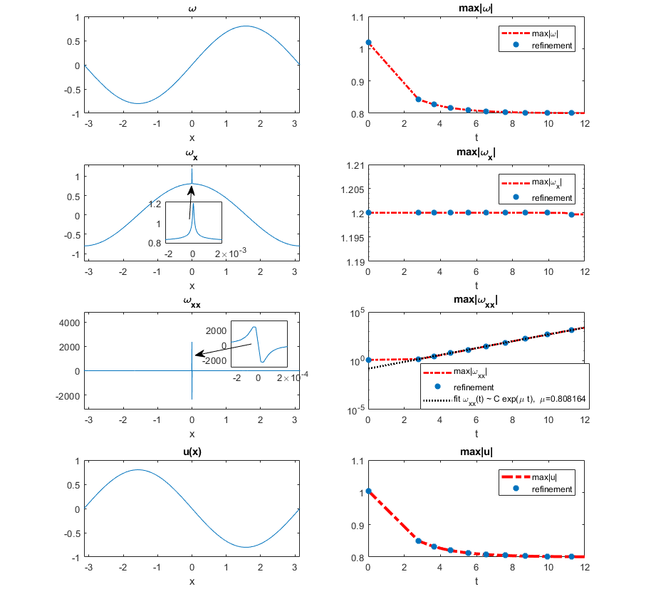
Figure 26: Results of the simulation of Eqs. (1) and (55) with $a=1$ and IC (83) as in Ref. Okamoto2008 showing $\omega(x)$, its derivatives $\omega_{x}(x)$, $\omega_{xx}(x)$, and $u(x)$ at $t\approx 12$ and the growth of their maximum values as functions of time.

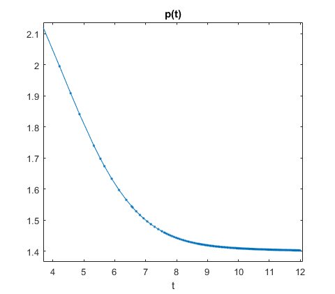
Figure 27: Left panel: Log-log plot of the Fourier spectrum $|\hat{\omega}_{k}|$ for the solution in Fig. 26 and a fit to the model (62). Center and right panels: Time dependence of $\delta(t)$ and $p(t)$ obtained from the fit to (62). Center panel also shows a fit of $\delta(t)$ to the stretched exponential model $\delta(t)\sim e^{-\kappa t^{\nu}}$.

The second type of IC we used for $a=1$ is given by

$$\omega_{0}(x)=\sin(x)+0.1\sin(2x),$$ (83)

which is the same as in Ref. Okamoto2008 . It allows us to directly compare the results of our simulations with Ref. Okamoto2008 . We obtain exactly the same plots as in Fig. 1 of Ref. Okamoto2008 , see Fig. 26. The difference between simulations with IC (82) and IC (83) are seen by comparing Figs. 25 and 26. For example, the spatial derivatives of $\omega$ approach discontinuities at $x=0$ in Fig. 25 vs. $x=\pm\pi$ in Fig. 26. The AAA rational approximation shows an approach of two vertical branch cuts to $x=0$ over time, so the spectrum is not oscillatory and we are able to easily recover $\delta(t)$ and $p(t)$ from the fit to Eq. (62). The fits show a stretched-exponential in time approach of the singularity to the real line i.e., $\delta(t)\sim e^{-\kappa t^{\nu}}$, see Fig. 27 (middle panel). Figure 27 (middle and right panels) showing $\delta(t)$ and $p(t)$ can be compared with Fig. 3(a,b) of Ref. Okamoto2008 . Our values of $\delta(t)$ match those values from Fig. 3(a) of Ref. Okamoto2008 well, while values of $p(t)$ do not match precisely with Fig. 3(b) of Ref. Okamoto2008 because they marginally depend on the particular part of spectrum $|\hat{\omega}_{k}|$ that is used for the fitting.

For $a>1$ with IC (82), we observe global existence of the solution. Its initial expansion in $x$-space is arrested by the periodic boundary conditions with an infinite slope forming at the boundary $x=\pm\pi$ so that $\max\limits_{x}|\omega_{x}|\rightarrow{\infty}$ as $t\rightarrow{\infty}$ (although $\max\limits_{x}|\omega|,\max\limits_{x}|u|,|\omega_{x}(x=0)|\rightarrow{0}$ as $t\rightarrow{\infty}$). The complex singularities approach the real line in infinite time. Their positions scale like $x_{sing}\sim\pm\pi\pm\mathrm{i}y_{0}\exp{(-\kappa_{2}t^{\nu_{2}})}$, where $y_{0},\kappa_{2},\nu_{2}>0$. When $a\to 1^{+}$, we observe that $\max\limits_{x}|\omega|$ grows for a short time and then decays. Unlike the $x\in\mathbb{R}$ case, it is relatively easy to compute accurately for $a\to 1^{+}$ and we have been able to obtain numerical evidence of global existence for $a$ as small as 1.000001. For IC (83), we also observe global existence of the solution with decay of $\max\limits_{x}|\omega|$ and unbounded growth of $|\omega_{x}(x=0)|$ as $t\to\infty.$ The complex singularities approach the real line like $x_{sing}\sim 0\pm\mathrm{i}y_{0}\exp{(-\kappa_{2}t^{\nu_{2}})}$, where $y_{0},\kappa_{2},\nu_{2}>0$.

We find the same behaviour of the kinetic energy for the periodic BC as in $x\in\mathbb{R}$ case described in Section 9 for $a\leq 0.95$, while for $a=1$ we have that $E_{K}\to const$ as $t\to\infty$ (because $\max\limits_{x}|u|\to const$ as $t\to\infty$) and for $a>1$ we have that $E_{K}\to 0$ as $t\to\infty$ (because $\max\limits_{x}|u|\to 0$ as $t\to\infty$).

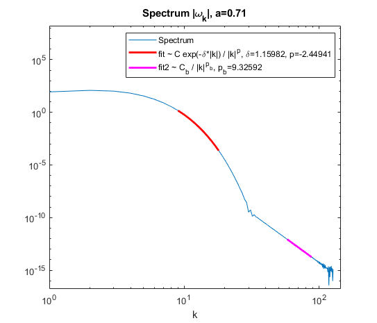
Figure 28: The Fourier spectrum $|\hat{\omega}_{k}|$ of the self-similar profile (9) for $a=0.71$ obtained by GPM iterations (74) of Eq. (84). Two fits are shown in different ranges of $k$ with the first fit to Eq. (62) with $\delta\neq 0$ at intermediate $k$ and the second a power law fit $\propto|k|^{-p_{b}}$ for larger $|k|$. Left panel: Log-linear plot where the first fit turns into a nearly linear function. Right panel: Log-Log plot where the second fit turns into a nearly linear function.

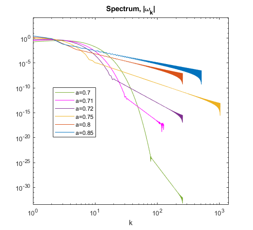
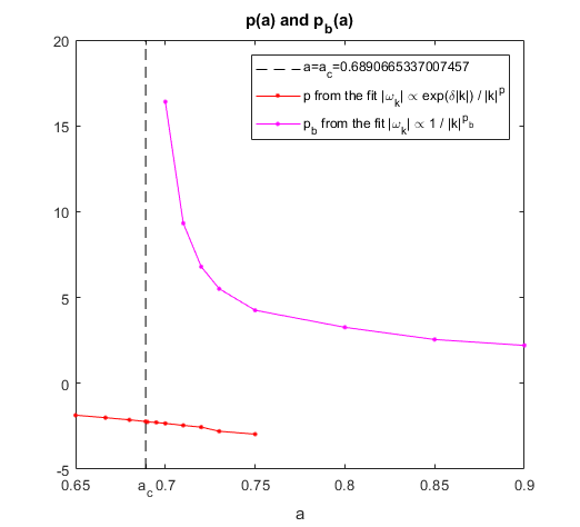
Figure 29: Left panel: The Fourier spectra $|\hat{\omega}_{k}|$ of the self-similar profile (9) for various values of $a$ as in the Table 2 obtained by GPM iterations (74) of Eq. (84). Right panel: $p(a)$ and $p_{b}(a)$ from the Table 2 extracted from the two fits as in Fig. 28.

Self-similar profiles from GPM. We also numerically computed the self-similar profile $f(x)$ in Eq. (9) for $a_{c}<a\leq 0.85$ using GPM described in Section 9 with $\alpha=0$. In contrast to Section 9, we do not need to use the coordinate transformation (66) because $f(x)$ is now $2\pi$-periodic with $\xi\equiv x$. We used GPM to solve Eq. (46) by the iteration (74) with ${\mathcal{M}}f$ and ${\mathcal{N}}[f]f$ from Eq. (67) replaced by

$$\begin{split}&{\mathcal{M}}f:=f=-agf_{x}+f{\mathcal{H}}^{2\pi}f:={\mathcal{N}}[f]f,\quad\\ &g_{x}={\mathcal{H}}^{2\pi}f.\end{split}$$ (84)

The matrix $\bf\ M$ used in Eq. (74) now turns into the identity matrix. We do not need to solve the nonlinear eigenvalue problem for $\alpha$ because now $\alpha\equiv 0$. While performing the iteration (74), we had to reduce $\Delta\tau$ even more than in Section 9 to make sure the iterations converged and also had to use more Fourier modes in the spectrum, since the spectrum decay is only algebraic for these solutions. Due to these technical limitations we were unable to explore the range $0.85<a<1$, but we fully expect that self-similar solutions exist there because time-dependent simulations converge to self-similar profiles, at least over the lower range $a_{c}<a\lesssim 0.95$ (see Fig. 22). It was not possible to obtain convergence in the upper range $0.95\lesssim a<1$ because the solution spectrum quickly widened, and we were unable to reach the self-similar regime before the computation became prohibitively slow. The behavior of solutions (blow up vs. global existence) therefore remains unknown in this range. We conjecture that blow up occurs for all $a_{c}<a<1$ with global existence only for $a=1$ (as demonstrated) and for larger values of $a$.

The Fourier spectrum of $|\hat{\omega}_{k}|$ corresponding to the self-similar profile (9) has two distinct domains for $|k|\gg 1$. The particular case $a=0.71$ shown in Fig. 28 depicts such domains. The first domain corresponds to complex singularities of Theorem 1 (Eq. (21)) located at $x_{sing}=\pm\mathrm{i}\delta.$ This domain is well fitted by Eq. (62). From this fit we find that $\delta=1.15982$ and $p=-2.44941$, as shown in Fig. 28. Using Eqs. (21) and (63) we obtain the prediction of Theorem 1 that $p=\frac{-a}{1-a}=-2.44827\ldots$ which agrees within an accuracy of $<0.05\%$ with the numerical fit to Eq. (62). The second domain is due to complex singularities located at $x=\pm\pi$ and results in a discontinuity of high-order derivatives of $\omega(x)$ at the periodic boundary. This domain has the power law spectrum $\propto|k|^{-p_{b}}$(i.e., in Eq. (62) it corresponds to $\delta=0$ and $p=p_{b}$) which is dominant for larger $|k|$. In the particular case of Fig. 28, we obtain $p_{b}=9.32592\ldots.$ This implies that the 9th and higher-order derivatives of $\omega(x)$ have a discontinuity at the periodic boundary. All these singularities can be seen using the AAA algorithm described in Section 10. We also find that as $a$ approaches to $a_{c}$ from the right, i.e. $a\rightarrow{a_{c}^{+}}$, increasingly higher order derivatives experience discontinuities at the periodic boundary, i.e. $p_{b}\rightarrow{\infty}$ as $a\rightarrow{a_{c}^{+}}$, see Fig. 29 (right panel). These solutions with finite smoothness at the periodic boundary can be considered the analog of the self-similar solutions with compact support found in Sections 8 and 9, for solutions on the real line with $a_{c}<a\leq 1$.

Table 2 provides the values of $\delta,p$ and $p_{b}$ for various values of parameter $a$ obtained from the fits described above. We note that the symmetry (51) is not valid for periodic BC. Thus, the parameter $\delta$ is now fixed for each $a$, contrary to the case $x\in\mathbb{R}$ where it is a free parameter, cf. Section 9.

Table 2: Table of values of $\delta,p$ and $p_{b}$ extracted via a fit of spectra $|\hat{\omega}_{k}|$ to the model (62), obtained from eigenvalue problem simulations of Eq. (84) for various values of $a$, $a_{c}<a<1$. $\delta$ and $p$ are extracted from the fit $|\hat{\omega}_{k}|\propto\exp(-\delta|k|)/|k|^{p}$ to the central part ($k\sim 0$) of the spectrum and $p_{b}$ is extracted from the fit $|\hat{\omega}_{k}|\propto 1/|k|^{p_{b}}$ in the tails ($k\gg 1$) of the spectrum. Simulations with $a\geq 0.71$ were performed in double precision arithmetic. To see the power law tail of the spectrum and extract $p_{b}$ in the case of $a=0.7$ we had to use quadruple precision. For $a_{c}<a\leq 0.695$ the power law tail was not observable even in quadruple precision. See Fig. 29 for the spectra and plots of $p(a)$ and $p_{b}(a)$. The accuracy of $\delta,p$ and $p_{b}$ approximately corresponds to the number of digits provided in the table.

$a$	$\delta$	$p$	$p_{b}$
0.69	0.2338	-2.2446	-
0.695	0.5954	-2.2787	-
0.7	0.8177	-2.3333	16.407
0.71	1.1598	-2.4494	9.3259
0.72	1.44	-2.55	6.81
0.73	1.73	-2.79	5.51
0.75	2.20	-2.96	4.26
0.8	-	-	3.26
0.85	-	-	2.55
0.9	-	-	2.21

Here we summarize the solution behaviour of Eqs. (1) and (55) for $x\in[-\pi,\pi]$ and generic smooth IC depending on the parameter $a$:

• $a<a_{c}:$ Behaviour of solutions is the same at $t\to t_{c}$ as for the $x\in\mathbb{R}$ case, with collapse as in Eq. (6).

• $a_{c}<a\lesssim 0.95:$ Blow up both in $\omega$ and $u$ in finite time $t_{c}$ with solution approaching the universal self-similar profile (9) as $t\to t_{c}$. That profile $f(x)$ has discontinuities in the high-order derivatives with complex singularities touching the real line only at $x=\pm\pi$. The number of continuous derivatives becomes infinite in the limit $a\to a_{c}^{+}$. The singularities approach the real line as $x_{sing}\simeq\pm\pi\pm\mathrm{i}(t_{c}-t)^{\alpha_{3}}y_{b}$, where $\alpha_{3}(a)>0$.

• $a=1:$ Global existence of solution with a singularity approaching the real line exponentially in time. For both IC (82) and IC (83) we find $\max\limits_{x}|\omega|,\max\limits_{x}|u|,\max\limits_{x}|u_{x}|\rightarrow{const}$, $\max\limits_{x}|\omega_{x}|=|\omega_{x}(x=0)|=const$, and $\max\limits_{x}|\omega_{xx}|\rightarrow{\infty}$ as $t\rightarrow{\infty}$.

• $a>1:$ Global existence of solution with a singularity approaching the real line exponentially in time. For IC (82) the singularity approaches the real line near $x=\pm\pi$ and $\max\limits_{x}|\omega|,\max\limits_{x}|u|,|\omega_{x}(x=0)|\rightarrow{0}$ and $\max|\omega_{x}|\rightarrow{\infty}$ as $t\rightarrow{\infty}$.

12 Conclusions and discussion

We have performed a systematic sweep of the parameter $a$ in the generalized CLM equation (1) to determine the possibility of singularity formation and, when it occurs, its type, i.e., collapse vs. blow-up. We identified a new critical value $a=a_{c}=0.6890665337007457\ldots$ such that for $a<a_{c}$ collapse occurs both on the real line $x\in\mathbb{R}$ and for periodic BC. Here, collapse means that not only is there a finite time singularity in which the amplitude of the solution $\omega(x,t)$ tends to infinity, but there is also a catastrophic shrinking of the spatial extent of the solution to zero as $t\to t_{c}$, described by the self-similar form (6). In the intermediate range $a_{c}<a\leq 1,$ we found there is finite-time singularity formation for $x\in\mathbb{R}$, with the self-similar solution (6) experiencing an infinite rate of expansion as $t\to t_{c}$. This type of self-similar singularity formation, in which the spatial domain does not collapse, is termed ‘blow up’. The power $\alpha$ in Eq. (6) controls collapse (for $\alpha>0,\ a<a_{c})$ vs. blow up ($\alpha\leq 0,\ a\geq a_{c})$. We elucidated the dependence of $\alpha(a)$ on $a$ via both direct numerical simulation of Eq. (1) and the solution of a nonlinear eigenvalue problem (46) using the generalized Petviashvili method (74). We have also performed multiprecision simulations (up to 68 digits of accuracy) to demonstrate the possibility of recovering $\alpha(a)$ and the structure of self-similar solutions with any desired precision.

We show that collapsing solutions of (1) have finite energy $E_{K}$ up to and including the critical time $t_{c}$ for $a<0.265\pm 0.001$. Such finite energy solutions are of interest in analogy with the problem concerning global regularity of the 3D Euler and Navier-Stokes equations with smooth initial data, see Refs. FeffermanMilleniumprize2006 ; GibbonPhysD2008 . We found for general values of $a$ that the self-similar solution (6) is real analytic for $a<a_{c}$ while it has finite support for $a_{c}<a\leq 1.$

We identified that the blow up for periodic BC with $a_{c}<a\leq 0.95$ is qualitatively different from that for $x\in\mathbb{R}$, because the periodic BC arrests or blocks the unbounded spatial expansion of the solution on the real line. To our surprise, such arrest does not result in the global existence of the solution but instead leads to a new form of self-similar blow-up (9), in which weak singularities develop at the boundaries of the periodic domain. In the limit $a\to a_{c}^{+},$ this self-similar solution turns into an infinitely smooth ($C^{\infty}$) solution. We believe that the qualitative difference in blow up between $x\in\mathbb{R}$ and periodic BC might serve as an interesting lesson relevant to the search for singularities in the 3D Euler equation.

Both self-similar solutions (6) and (9) are nonlinearly stable, as follows from our simulations. Quite generic classes of IC converge to these solutions during the temporal evolution. In the case of Eq. (6), such convergence/stability is understood in the sense of convergence to a family of self-similar solutions, up to a rescaling in $x$, because of the symmetry (51) of Eq. (46).

The structure of the leading order singularities in the complex plane $x$ (which is the analytical continuation from $x\in\mathbb{R}$) is determined by Theorem 1. That result is valid for both $x\in\mathbb{R}$ and periodic BC and is in full agreement with simulations. For $a<a_{c}$ the leading order singularities are the closest singularities to the real line in the complex $x$-plane. For $a>a_{c}$, these singularities still determine the structure of self-similar solutions near $x=0$, while the solution near the boundaries of finite support in $x\in\mathbb{R}$ and the periodic boundaries for periodic BC are controlled by less singular terms. The self-similar solution profiles for these $a$ have been found with high accuracy by solving a nonlinear eigenvalue problem. We have also proved in Theorem 3 that, except for the exact closed-form solutions for $a=0$ and $a=1/2$, the analytical structure of singularities in the complex $x$-plane goes beyond the leading order singularities. In particular, we numerically identified using the AAA algorithm the existence of additional, non-leading-order branch points for $a\neq 0,1/2$.

We found from our simulations that quite generic IC result in the global existence of solutions for $a\gtrsim 1.3$ and $x\in\mathbb{R}$, while for periodic BC global existence is ensured for $a\geq 1.$ In the remaining gaps $1<a\lesssim 1.3$ for $x\in\mathbb{R}$ and $0.95<a<1$ for the periodic case, our simulations are inconclusive and unable to distinguish between singularity formation and global existence. We believe that more concrete results in this range of $a$ will require additional analysis and/or substantial efforts in simulation.

We suggest that among many other issues, the following questions would be interesting to address in future work:

1. Analytical study of the complex singularities beyond the leading order singularities addressed in Theorem 1. In particular, the case $a=2/3$ might be especially interesting because the leading order singularity is very simple, namely, a third order pole.

2. Either extend GPM to the compactly supported case $a>a_{c}$ for $x\in\mathbb{R}$, or use a version of the method in Ref. ChenHouHuang based on cubic splines. However, splines generally lose information about the analyticity of solutions in the complex plane. One way to improve the performance of GPM in this range of $a$ might be to use a coordinate transform in the form of a conformal mapping which would simultaneously resolve the numerical grid near $x=\pm x_{b}$ while keeping the analyticity of the solution intact. This type of approach has been suggested in Ref. LushnikovDyachenkoSilantyevProcRoySocA2017 .

3. Fill the gaps in our knowledge on blow up vs. global existence of solutions in the parameter regime $1<a\lesssim 1.3$ for $x\in\mathbb{R}$ and $0.95<a<1$ for periodic BC.

4. Look for possible analytical continuation/bifurcation at $a=a_{c}$ between self-similar solutions (6) for the case $x\in\mathbb{R}$ and Eq. (9) for periodic BC.

5. Perform an analysis of the nonlinear stability of the blow-up solutions. This could be qualitatively similar to the stability of collapse in PDEs such as the nonlinear Schrödinger equation and the Patlak-Keller-Segel equation, see e.g. Refs. ZakharovJETP1972 ; ChPe1981 ; SulemSulem1999 ; BrennerConstantinKadanoff1999 ; KuznetsovZakharov2007 ; LushnikovDyachenkoVladimirovaNLSloglogPRA2013 .

6. Analyze the formation of singularities at the initial time $t=0^{+}$. This can give information on the type of singularities which first form in the complex plane, and subsequently move toward the real line. Such an analysis has been previously performed for the evolution of a vortex sheet in the Kelvin-Helmholtz problem CowleyBakerTanveerJFM1999 , which is also governed by a nonlocal PDE. However, a significant difference between the current problem and the vortex sheet problem is that here the singularities initially form at infinity in the complex plane, whereas in the vortex sheet problem they are generated at finite locations, due to a singularities in the kernel of the nonlocal term at these locations.

Conflict of interest

The authors declare that they have no conflict of interest.

Appendix A Hilbert transform for transformed variable

In this Appendix we derive the expression for the Hilbert transform in the auxiliary variable $q$ (52) of Section 7.

The change of variable (52) in Eq. (2) together with (53) results in

$${\mathcal{H}}f(x)=\frac{1}{\pi}\text{p.v.}\int^{\infty}_{-\infty}\frac{f(x^{\prime})}{x-x^{\prime}}\mbox{d}x^{\prime}=\frac{1}{\pi}\text{p.v.}\int^{\pi}_{-\pi}\frac{\tilde{f}(q^{\prime})}{\tan{\frac{q}{2}}-\tan{\frac{q^{\prime}}{2}}}\frac{\mbox{d}q^{\prime}}{2\cos^{2}{\frac{q^{\prime}}{2}}}$$

$$=\frac{1}{2\pi}\text{p.v.}\int^{\pi}_{-\pi}\frac{\tilde{f}(q^{\prime})\left[1+\tan{\frac{q}{2}}\tan{\frac{q^{\prime}}{2}}-\tan{\frac{q^{\prime}}{2}}\left(\tan{\frac{q}{2}}-\tan{\frac{q^{\prime}}{2}}\right)\right]}{\tan{\frac{q}{2}}-\tan{\frac{q^{\prime}}{2}}}\mbox{d}q^{\prime}$$

$$=\frac{1}{2\pi}\text{p.v.}\int^{\pi}_{-\pi}\frac{\tilde{f}(q^{\prime})}{\tan{\left(\frac{q-q^{\prime}}{2}\right)}}\mbox{d}q^{\prime}-\frac{1}{2\pi}\int\limits^{\pi}_{-\pi}{\tilde{f}}(q^{\prime})\tan{\frac{q^{\prime}}{2}}\mbox{d}q^{\prime}={\mathcal{H}}^{2\pi}f(q)+C^{2\pi}_{f},$$ (85)

where we used the identities

$$\tan{(a-b)}=\frac{\tan{a}-\tan{b}}{1+\tan{a}\tan{b}}\quad\text{and}\quad\frac{1}{\cos^{2}{\frac{q}{2}}}=\tan^{2}{\frac{q}{2}}+1$$

as well as the definitions (55) and (56). Eq. (A) ensures that $\lim\limits_{q\to\pm\pi}[{\mathcal{H}}^{2\pi}f(q)+C^{2\pi}_{f}]=0.$

Also ${\mathcal{H}}^{2\pi}f(x)$, Eq. (55), is the reduction of ${\mathcal{H}}f(x)$, Eq. (2), to the class of $2\pi$-periodic functions. Assuming that $f(x)$ is the periodic function with the period $2\pi$, we obtain from Eq. (2) that

$${\mathcal{H}}f(x)=\frac{1}{\pi}\sum\limits_{n=-\infty}^{\infty}\text{p.v.}\int^{\pi}_{-\pi}\frac{f(x^{\prime})}{x-x^{\prime}+2\pi n}\mbox{d}x^{\prime}=\frac{1}{2\pi}\text{p.v.}\int^{\pi}_{-\pi}\frac{f(x^{\prime})}{\tan{\left(\frac{x-x^{\prime}}{2}\right)}}\mbox{d}x^{\prime}=:{\mathcal{H}}^{2\pi}f(x),$$ (86)

where we used the definition (55) and the identity

$$\sum\limits^{\infty}_{n=-\infty}\frac{1}{x+2\pi n}=\frac{1}{2\tan{\frac{x}{2}}}.$$ (87)

References

- (1) Alpert, B., Greengard, L., Hagstrom, T.: Rapid evaluation of nonreflecting boundary kernels for time-domain wave propagation. SIAM J. Num. Anal. 37, 1138–1164 (2000)
- (2) Baker, G., Caflisch, R.E., Siegel, M.: Singularity formation during Rayleigh–Taylor instability. Journal of Fluid Mechanics 252, 51–78 (1993)
- (3) Brenner, M.P., Constantin, P., Kadanoff, L.P., Schenkel, A., Venkataramani, S.C.: Diffusion, attraction and collapse. Nonlinearity 12(4), 1071–1098 (1999)
- (4) Carrier, G.F., Krook, M., Pearson, C.E.: Functions of a Complex Variable. McGraw-Hill, New York (1966)
- (5) Castro, A., Córdoba, D.: Infinite energy solutions of the surface quasi-geostrophic equation. Adv. Math. 225(4), 1820–1829 (2010)
- (6) Chen, J.: Singularity formation and global well-posedness for the generalized Constantin–Lax–Majda equation with dissipation. Nonlinearity 33(5), 2502 (2020)
- (7) Chen, J., Hou, T.Y., Huang, D.: On the finite time blowup of the De Gregorio model for the 3D Euler equation. arXiv:1905.06387 (2019)
- (8) Childress, S., J.K., P.: Nonlinear aspect of chemotaxis. Math. Bio. 56, 217–237 (1981)
- (9) Constantin, P., Lax, P.D., Majda, A.: A simple one-dimensional model for the three-dimensional vorticity equation. Commun. Pure Appl. Math. 38(6), 715–724 (1985)
- (10) Cooper, G.J., Verner, J.H.: Some Explicit Runge-Kutta Methods of High Order. SIAM Journal on Numerical Analysis 9(3), 389–405 (1972). DOI 10.1137/0709037. URL https://doi.org/10.1137/0709037
- (11) Cowley, S.J., Baker, G.R., Tanveer, S.: On the formation of Moore curvature singularities in vortex sheets. J. Fluid Mech. 378, 233–267 (1999)
- (12) De Gregorio, S.: On a one-dimensional model for the three-dimensional vorticity equation. J. Stat. Phys. 59(5-6), 1251–1263 (1990)
- (13) Dyachenko, A.I., Dyachenko, S.A., Lushnikov, P.M., Zakharov, V.E.: Dynamics of Poles in 2D Hydrodynamics with Free Surface: New Constants of Motion. Journal of Fluid Mechanics 874, 891–925 (2019)
- (14) Dyachenko, S.A., Lushnikov, P.M., Korotkevich, A.O.: The complex singularity of a Stokes wave. JETP Letters 98(11), 767–771 (2013). DOI 10.7868/S0370274X13230070
- (15) Dyachenko, S.A., Lushnikov, P.M., Korotkevich, A.O.: The complex singularity of a Stokes wave. JETP Letters 98(11), 675–679 (2013). DOI 10.7868/S0370274X13230070
- (16) Dyachenko, S.A., Lushnikov, P.M., Korotkevich, A.O.: Branch Cuts of Stokes Wave on Deep Water. Part I: Numerical Solution and Padé Approximation. Studies in Applied Mathematics 137, 419–472 (2016). DOI DOI:10.1111/sapm.12128
- (17) Dyachenko, S.A., Lushnikov, P.M., Vladimirova, N.: Logarithmic scaling of the collapse in the critical Keller-Segel equation. Nonlinearity 26, 3011–3041 (2013)
- (18) Elgindi, T.M.: Finite-time singularity formation for solutions to the incompressible Euler equations on . arXiv:1904.04795 (2019)
- (19) Elgindi, T.M., Jeong, I.J.: Finite-time singularity formation for strong solutions to the axi-symmetric 3D Euler equations. Ann. PDE 5(2), 1–51 (2019)
- (20) Elgindi, T.M., Jeong, I.J.: On the effects of advection and vortex stretching. Archive for Rational Mechanics and Analysis 235, 1763–1817 (2020). DOI 10.1007/s00205-019-01455-9. URL https://doi.org/10.1007/s00205-019-01455-9
- (21) Fefferman, C.L.: Existence and smoothness of the Navier-Stokes equation. The millennium prize problems pp. 57–67 (2006)
- (22) Gibbon, J.D.: The three-dimensional Euler equations: Where do we stand? Physica D 237, 1894–1904 (2008)
- (23) Hou, T.Y., Jin, T., Liu, P.: Potential singularity for a family of models of the axisymmetric incompressible flow. J. Nonlinear Sci. 28(6), 2217–2247 (2018)
- (24) Hou, T.Y., Lei, Z., Luo, G., Wang, S., Zou, C.: On finite time singularity and global regularity of an axisymmetric model for the 3D Euler equations. Archive for Rational Mechanics and Analysis 212(2), 683–706 (2014)
- (25) Hou, T.Y., Li, C.: Dynamic stability of the three-dimensional axisymmetric Navier-Stokes equations with swirl. Commun. Pure Appl. Math. 61(5), 661–697 (2008)
- (26) Hou, T.Y., Li, R.: Dynamic depletion of vortex stretching and non-blowup of the 3-D incompressible Euler equations. J. Nonlinear Sci. 16(6), 639–664 (2006)
- (27) Hou, T.Y., Shi, Z., Wang, S.: On singularity formation of a 3D model for incompressible Navier-Stokes equations. Adv. Math. 230(2), 607–641 (2012)
- (28) Kuznetsov, E.A., Zakharov, V.E.: Wave Collapse. World Scientific Publishing Company, New York (2007)
- (29) Lakoba, T.I., Yang, J.: A generalized Petviashvili iteration method for scalar and vector Hamiltonian equations with arbitrary form of nonlinearity. J. Comput. Phys. 226, 1668–1692 (2007)
- (30) Lei, Z., Hou, T.Y.: On the stabilizing effect of convection in three-dimensional incompressible flows. Commun. Pure Appl. Math. 62(4), 501–564 (2009)
- (31) Lei, Z., Liu, J., Ren, X.: On the Constantin–Lax–Majda model with convection. Comm. Math. Phys. pp. 1–19 (2019)
- (32) Lushnikov, P.M.: Dispersion-managed soliton in a strong dispersion map limit. Opt. Lett. 26, 1535 – 1537 (2001)
- (33) Lushnikov, P.M., Dyachenko, S.A., Silantyev, D.A.: New conformal mapping for adaptive resolving of the complex singularities of Stokes wave. Proc. Roy. Soc. A 473, 20170198 (2017)
- (34) Lushnikov, P.M., Dyachenko, S.A., Vladimirova, N.: Beyond leading-order logarithmic scaling in the catastrophic self-focusing of a laser beam in Kerr media. Phys. Rev. A 88, 013845 (2013)
- (35) Lushnikov, P.M., Silantyev, D.A., Siegel, M.: Collapse vs. blow up and global existence in the generalized Constantin-Lax-Majda equation. arXiv:2010.01201 (2020)
- (36) Nakatsukasa, Y., Sète, O., Trefethen, L.N.: The AAA algorithm for rational approximation. SIAM J. Sci. Comp. 40(3), A1494–A1522 (2018)
- (37) Okamoto, H., Ohkitani, K.: On the role of the convection term in the equations of motion of incompressible fluid. J. Phys. Soc. Japan 74(10), 2737–2742 (2005)
- (38) Okamoto, H., Sakajo, T., Wunsch, M.: On a generalization of the Constantin–Lax–Majda equation. Nonlinearity 21(10), 2447 (2008)
- (39) Pelinovsky, D., Stepanyants, Y.: Convergence of petviashvili’s iteration method for numerical approximation of stationary solutions of nonlinear wave equations. SIAM J. Numer. Anal. 42, 1110–1127 (2004)
- (40) Petviashvili, V.I.: Equation for an extraordinary soliton. Sov. J. Plasma Phys. 2, 257–258 (1976)
- (41) Stein, E.M.: Singular integrals and differentiability properties of functions, vol. 2. Princeton university press (1970)
- (42) Sulem, C., Sulem, P.L.: Nonlinear Schrödinger Equations: Self-Focusing and Wave Collapse. World Scientific, New York (1999)
- (43) Sulem, C., Sulem, P.L., Frisch, H.: Tracing complex singularities with spectral methods. J. Comput. Phys. 50, 138–161 (1983)
- (44) Yang, J.: Nonlinear Waves in Integrable and Nonintegrable Systems. SIAM (2010)
- (45) Zakharov, V.E.: Collapse of langmuir waves. Sov. Phys. JETP 35, 908 (1972)