Quadratic Funding and Matching Funds Requirements

Abstract

In this paper we examine the mechanism proposed by Buterin, Hitzig, and Weyl (2019) for public goods financing, particularly regarding its matching funds requirements, related efficiency implications, and incentives for strategic behavior. Then, we use emerging evidence from Gitcoin Grants, to identify stylized facts in contribution giving and test our propositions. Because of its quadratic design, matching funds requirements scale rapidly, particularly by more numerous and equally contributed projects. As a result, matching funds are exhausted early in the funding rounds, and much space remains for social efficiency improvement. Empirically, there is also a tendency by contributors to give small amounts, scattered among multiple projects, which accelerates this process. Among other findings, we also identify a significant amount of reciprocal backing, which could be consistent with the kind of strategic behavior we discuss.

Keywords— quadratic funding, public goods, Gitcoin

JEL codes— D47, D61, D71, H41

Introduction

The efficient provision of public goods is certainly a central issue for the economy of any community, ecosystem, or society. The economic literature recognizes that goods such as open-source software, knowledge, and urban public equipment, are characterized by non-exclusion and non-rivalry properties. When the allocation of these goods is decentralized, these characteristics lead to their under-provision (Samuelson 1954). On the other hand, the centralized provision of public goods, faces the challenge of identifying the preferences of the individuals the public good is aimed to benefit (Clarke 1971; Groves 1973). In addition, in many settings, there is the additional problem that the planner must choose between a variety of public goods that could be financed.

Buterin, Hitzig, and Weyl (2019) (BHW) has recently proposed a decentralized matching funding mechanism for such a setting, that, under certain conditions, has the property of achieving an “optimal provision for an ecosystem of public goods”. The mechanism, known as quadratic funding (QF), involves a sponsor (i.e., donor, or group of sponsors) matching the contributions of a (decentralized) community of individuals that support the creation of public good projects. In this mechanism, total funds to be received by a public good project (i.e., the size of the public good) results from applying the quadratic rule to the individual contributions (i.e., from taking the sum of the square-roots of individual contributions and then taking the square of this value) and using the sponsor funds to reach the resulting levels. As the mechanism pays projects additional funding in proportion to funds committed by other sources, it also resembles other matching funds mechanisms observed, for example in philanthropic giving, public infrastructure funding, and public-private startup funding.

The ability of this innovative mechanism to achieve social optimality through a decentralized arrangement immediately attracted the attention of both academics and practitioners, which have put the mechanism into real applications. Probably the most notable of these is Gitcoin Grants (https://gitcoin.co/grants/), a financing platform for open-source software projects related to the Ethereum blockchain ecosystem. Gitcoin regularly uses the QF mechanism to allocate grants, and has been a center for discussion and dissemination of the mechanism.

One of the characteristics of the mechanism, as we discuss in this paper, is related to the fact that pools of funds provided by donors will be typically limited in relation to those needed to reach socially optimal allocations. In practice, the total funding that a project should receive according to the QF rule will be greater than the matching funds available in the donor pool. In other words, the mechanism will be typically subject to a limited pool of matching funds constraint. It therefore seems important to examine the properties of this mechanism in such a scenario. How much is efficiency compromised by the donors’ funding constraint? What would be an optimal allocation rule under limited funds and to what extent is it being met by the mechanism?

A second dimension of interest is related to possible strategic behavior from contributors, that might deteriorate the outcomes of the mechanism. BHW have pointed out forms of collusion and fraud as potential vulnerabilities and put forward ideas on their scope. Under what conditions does the mechanism incentivize strategic behavior by contributors? Into what degree behavior consistent with such incentives is observed?

Our aim is to further explore these questions at both the theoretical and empirical levels. Using emerging evidence from Gitcoin Grants, we will explore stylized facts related to contributors’ behavior and to the outcomes of funding rounds.

We start, in Section 1, by examining the question of what determines the size of the pool of matching funds to achieve optimality in the BHW sense. We note that required funds increase non-linearly with the number of contributors, and as result, any given pool of matching funds will be rapidly exhausted in most real applications. In addition, we will also note that required funds increase as contributors’ correlate their investment allocations across projects, an observation that could be significant in terms of platform design (e.g., designs that might induce correlations via behavioral effects).

This leads to the question about the efficiency of the mechanism under limited matching funds. In their paper, BHW recognize that “even the wealthiest philanthropists do not have infinite funds and, thus, cannot simply agree to finance arbitrarily large deficits”. Then, as an alternative, they discuss a variant on the QF mechanism (i.e., the “Capital Constrained QF Mechanism”), which limits the funding promised by the mechanism. Intuitively, this variant simply makes the public good as large as matching funds allow (i.e., large as to exhaust the matching pool). In this paper, we first note that, because of the mentioned matching requirements, this alternative mechanism is what will typically be feasible in practice. It is also the case of what has been implemented in Gitcoin Grants. In that platform, when the sum of required payments to each project exceeds available matching funds committed by donors, the subsidies to each project are scaled down by a constant so totals add up to the subsidy pool’s budget. As a result (i.e., if contributors perceive that matching funds will be scaled down to meet the funding constraint) individual contributions are lower than the socially optimal. Intuitively, this is because individuals are not fully compensated by the social benefits they generate from contributing to projects.

We next argue that, with limited matching funds, the relevant question is if the mechanism is able to optimally allocate those limited funds. In Section 2.2 we note that an optimal allocation of a limited pool of matching funds should equalize the marginal social benefits across projects. It turns out that this is not exactly the case with the CQF allocation, since the resulting allocation entails differences between the marginal benefits across projects. We show that this deviations from optimality will be higher: i) the lesser funds are available in the matching pool relative to matching requirements, ii) the higher the variability in the supporting preferences across projects (e.g., more equally invested projects imply higher marginal benefits than more concentrated projects), and iii) the higher the number of contributors.

Next, in terms of analyzing incentives to strategic behavior, in Section 3, we propose a simple formalization to analyze incentives for strategic behavior. In particular, we analyze incentives facing individuals raising funds in the mechanism (e.g., founders or team members of public good related projects) to contribute to other projects in the platform with the expectation of being invested back, a behavior we call reciprocal backing. We derive the conditions under which such a strategy is profitable and propose related hypotheses.

In the second part of the paper, we explore evidence from Gitcoin Grants 7th and 8th rounds, which took place during 19 days between September and October, 2020 and during 16 days in December 2020, respectively. In Section 4 we derive a series of stylized facts on individual contribution to projects, and examine some of the proposed theoretical hypotheses.

In Section 4.3, we document that, consistently with the theoretical intuition, QF target levels reached the funding constraint quite rapidly, particularly in the main round categories. In these categories this happened in less than four days, with a few reaching this value just in the second day. We will note that this observation has the implication that projects started to compete for funds very early in their rounds. We also confirm the theoretical insight that project matching fund requirements follow a quadratic relation with respect to the number of contributors.

Second, in Section 4.2, we show that projects’ matching requirements are somewhat aggravated by the fact that there is a tendency among contributors to make very small investments, scattered among multiple projects. This tendency can be seen, as we discuss, as one of the empirical characteristics of this mechanism, different from other documented crowdfunding mechanisms.

While such behavior is consistent with an interest of contributors in promoting many projects -powered by QF matching-, it could also result, as we mentioned, from strategic behavior. For example, we note that in the specific case of reciprocal backing, this strategy provides positive returns even when the pool of funds constraint is active. We document that at least 20% of contributions in the rounds analyzed are reciprocal, meaning that for every ten contributions to other projects by project team members, two are invested back by invested projects.

Finally, in Section 4.5, we specifically explore the question of whether contributors internalize the matching budget constraint. With this purpose, we estimate models that explain contribution amounts as a function of the matching budget constraint. We find a negative relationship, which in principle is consistent with the idea that individuals reduce their contributions as they perceive their projects of interest will receive fewer matching funds. We also explore an unexpected increase in the pool of matching funds that occurred during the 7th round. In this case, we find that contributors did not react by increasing their contributions. While this might be rather contradictory in first sight, we show that this result can be explained by the fact that although the pool of matching funds increased by 25%, due to the quadratic behavior of the mechanism, the effect on the matching budget constraint was negligible.

We end the paper with a discussion that reviews its main insights and suggests design implications.

Related literature

This paper is related to the literature that studies quadratic financing mechanisms for the optimal provision of public goods (Buterin, Hitzig, and Weyl 2019). The quadratic mechanism as a form of collective action pricing was proposed, and its equilibrium properties described, in Weyl (2012) and Lalley and Weyl (2019). Other antecedents of mechanisms based on quadratic mechanisms were proposed by Groves and Ledyard (1977) and Hylland and Zeckhauser (1979). The literature on mechanisms for nearly-optimal collective decision making is vast and one of its main references is the Vickrey – Clarke – Groves preferences revelation mechanism (Vickrey 1961; Clarke 1971; Groves 1973).

Arguably, QF can also be categorized as a form of crowdfunding. In crowdfunding, entrepreneurs raises external financing from a large audience (the“crowd”), in which each individual provides a very small amount (Belleflamme, Lambert, and Schwienbacher 2014). In exchange, individuals pre-order a product or receive a -small- share of future returns. While Gitcoin contributors do not receive shares of the projects they invest in, they are arguably the beneficiaries of the public goods (e.g., open source software, blockchain community growth, etc.) they fund. As it discusses characteristics of a form of crowdfunding the paper also aims to contribute to that literature (See, for instance, (Short et al. 2017; Agrawal, Catalini, and Goldfarb, n.d.; Burtch, Ghose, and Wattal 2015).

Finally, Gitcoin provides an example of an implementation of a new financing mechanism for open sources projects. In that sense, the paper adds, generally, to a vast literature that studies open source projects from an economic and management perspective (von Krogh and von Hippel 2006; Nagle 2019; August, Chen, and Zhu 2021), and specifically to financing issues related to these projects (Overney et al. 2020; Nakasai et al. 2017)

1 The QF rule and its matching fund requirements

The QF mechanism proposed by BHW is an allocation rule for the funding of public goods. Funding comes from the support of individual contributors plus an amount of matched funds provided by external donors. Under this mechanism, individual contributions are inputs to determine which and how much individual projects will be financed, while the external pool of matching funds serves to match individual decisions (i.e., no allocation decisions are made by external donors).

Assume that $p\in P$ indexes public good projects competing to receive funding. Also $i\in I$ indexes individual contributors. An individual $i$ supports a project $p$ by committing an amount of money $c_{i}^{p}$. We will examine the individual contributor decision problem below. For the moment, assume individual contributions from the $I$ individuals to the $P$ projects are known. In addition, assume there is a pool of funds provided by donors, that we will denote $D$, and that will be used to match individual contributions. For the moment assume that there is an endless pool of matching funds available (i.e., $D\rightarrow+\infty$).

In such a context, the QF rule allocates, for each project $p$, an amount of funds we denote $F^{p,\text{QF}}$, resulting from summing the square roots of all individual contributions, and taking the square of the result :

$$F^{p,\text{QF}}=\bigg{(}\sum_{i}\sqrt{c_{i}^{p}}\bigg{)}^{2}$$

Denote $C^{p}$ as the total funds committed by individual contributors to project $p$, i.e., $C^{p}=\sum_{i}c_{i}^{p}$. In order to satisfy the QF rule, project $p$ should additionally receive the target matching amount $M^{p,QF}$, defined by:

$$M^{p,QF}=F^{p,QF}-C^{p}$$

Figure 1 presents a graphical representation of the QF rule, first proposed in Buterin (2019). In the figure, total contributions by individuals ($C^{p}$) are represented by the blue shaded area. Required matching funds ($M^{p,QF}$) are represented by the gray shaded area. Total funds proposed by the QF rule ($F^{p,\text{QF}}$) are represented by size of the outer square (i.e., the sum of both blue and gray areas). The figure serves to illustrate the size of matching fund requirements, as well as the fact that the mechanism always requires positive external funds to work (i.e., there is no case in which positive matching funds are not required).

Figure 1: QF rule. A public good with four contributions $(c_{1},c_{2},c_{3},c_{4})$. The area of the outer square (i.e., sum of blue and gray areas) represents the size of the public good according to the QF rule $F^{p,\text{QF}}=(\sum\sqrt{c_{i}})^{2}$. Total funds contributed by individuals (i.e., $C^{p}=\sum_{i}c_{i}^{p}$) are represented by the sum of the blue square areas. Total required matching funds (i.e., $M^{p,QF}=F^{p,QF}-C^{p}$) are represented by the gray area.

Observation 1.1.

The total target matching amount $M^{p,QF}$ scales quadratically in the number of contributors.

It is useful to notice that the level of LR subsidy a project $p$ receives can also be expressed as:

$$M^{p,\text{QF}}=(\sum_{i}\sqrt{c_{i}^{p}})^{2}-\sum_{i}c_{i}^{p}=\\ \sum_{i}c_{i}^{p}+2\sum_{i\neq j}\sqrt{c_{i}^{p}c_{j}^{p}}-\sum_{i}c_{i}^{p}=2\sum_{i\neq j}\sqrt{c_{i}^{p}c_{j}^{p}}$$ (1)

This expression is useful because the summation has a number of terms equal to the number of pairs of contributors. So while total individual contributions ($C^{p}$) scale linearly, target matching amounts ($M^{p,\text{QF}}$) scale quadratically following the number of pairs of contributors, which corresponds to the combinatorial number $n\choose 2$ =$\frac{n!}{(n-2)!2!}=\frac{n(n-1)}{2}\approx\frac{n^{2}}{2}$.

In other words, the level of funding required to philanthropists needs to scale as fast as the square of the number of contributors. Note that this is certainly a demanding requirement (if not impossible) in any application with a considerable number of contributors.

Notice that the last expression of Equation 1 can also be identified using the same graphical representation. Figure 2 details that the target matching amount is comprised of set of rectangles of areas sized by $\sqrt{c_{i}^{p}c_{j}^{p}}$, and which sum a total area of $2\sum_{i\neq j}\sqrt{c_{i}^{p}c_{j}^{p}}$.

An alternative way of visualizing the requirements of the mechanism on the matching fund is to consider the requirements of the marginal contributor.

Observation 1.2.

A new contributor $j^{\prime}$ contributing $c_{j^{\prime}}^{p}$ to project $p$ will require the QF mechanism an additional match of $\sqrt{c_{k}^{p}}\bigg{(}2\sum_{i\neq k}\sqrt{c_{i}^{p}}\bigg{)}$.

In other words, an additional contributor places an increasingly demanding burden on the matching fund, since it demands the mechanism to match an amount that results from multiplying the new contribution by all existing contributions to the mechanism summed.

Figure 2: Representation of the target matching amount according to the QF rule. The size of the total matching amount, represented as the area in gray, is comprised of rectangles of areas sized by $\sqrt{c_{i}^{p}c_{j}^{p}}$, which sum $2\sum_{i\neq j}\sqrt{c_{i}^{p}c_{j}^{p}}$ as in Equation 1

1.0.1 Contribution patterns across projects and required matching funds

Finally, in inspecting the requirements on the matching fund it is also useful to consider how different patterns of contributions across projects pose different requirements to the matching fund.

Because of its quadratic design, given a fixed amount of total contributions $C^{p}$, the QF rule allocates a higher amount of matching funds to projects with more contributors (with smaller contributions). The flip side is that, from the point of view of fund requirements, holding target QF constant, more equally (less concentrated) invested projects require higher amounts of matching funding. This is expressed in the following proposition:

Proposition 1.3.

Denote $\alpha_{i}=\frac{\sqrt{c_{i}}}{\sum\sqrt{c_{i}}}$ as the share of total of the square roots of funds contributed by individual $i$ , and $\sigma^{2}$ a measure of the variability among shares (i.e., $\sigma^{2}=\frac{1}{n}\sum_{i}(\alpha_{i}-\bar{\alpha})^{2}$, where $\bar{\alpha}=\frac{1}{n}\sum_{i}\alpha_{i}$). Then, total matching fund requirements are given by

$$M^{p,\text{QF}}=(1-n\sigma^{2}-n\bar{\alpha}^{2})F^{p,\text{QF}}$$

As result, given a value of QF target, more equally invested projects require a higher amount of matching funds.

The proof is in the Appendix.

As a simple illustration of this, Figure 3 presents two projects, with a same QF target. Because Project 1 receives more equal contributions than Project 2 , it also requires more matching funds.

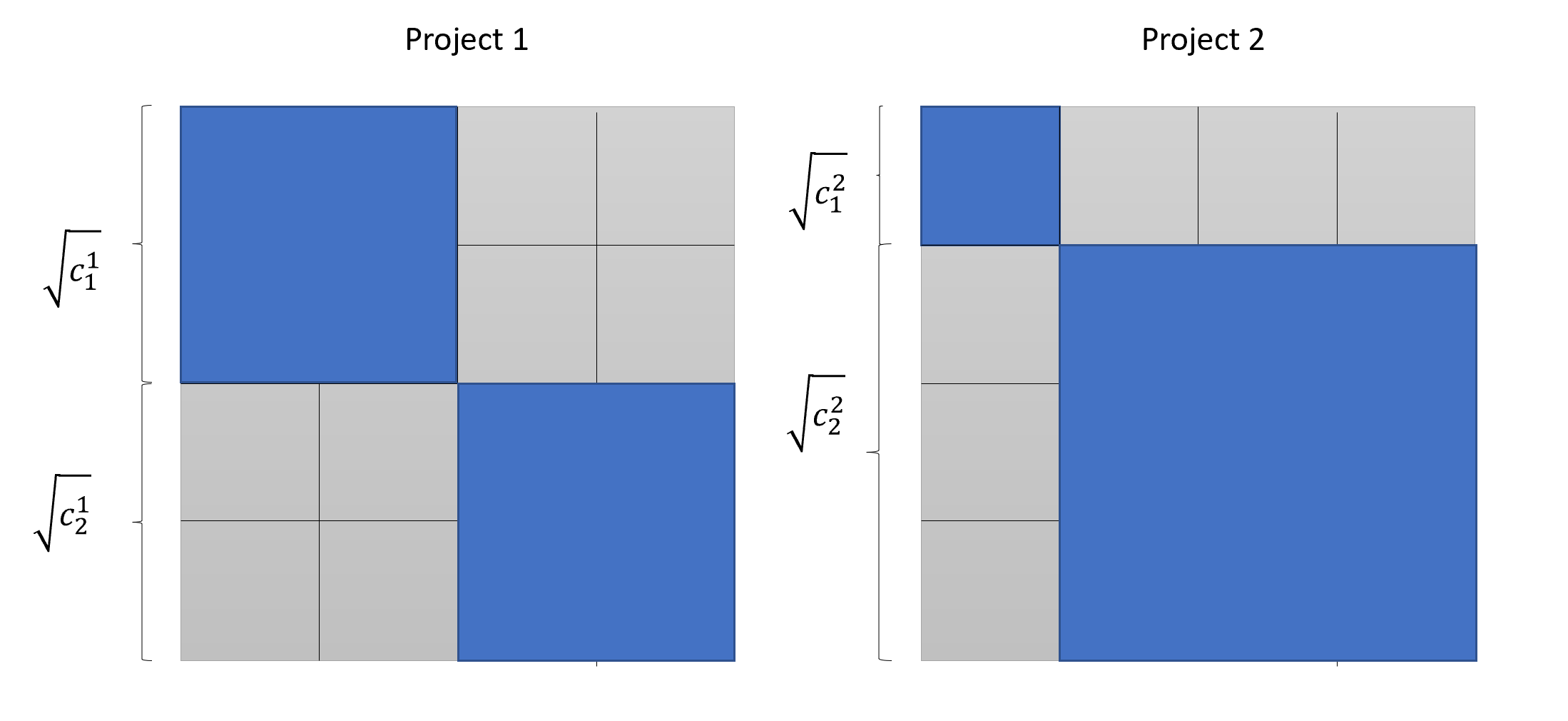
Figure 3: Two projects with equal QF funding targets. More equal contributions in Project 1 imply that this project requires a higher amount of matching funds

This leads to the question of how different patterns of contributions with individuals with given budgets will impact the matching requirements. Precisely, assume there are $N$ contributors, each with a budget $m_{i}$ to be invested across $P$ projects. Denote $s_{i}^{p}$ the share of funds that the individual contributor will allocate to project $p$ , so $\sum_{p}s_{i}^{p}=1$ $\forall i$.

One observation in this case is that matching requirements will be maximized if contributors’ preferences, as measured by their share of invested wealth, are perfectly correlated across individuals.

Proposition 1.4.

Given $N$ contributors, each having a budget of $m_{i}$ and allocating $s_{i}^{p}$ to project $p$, matching fund requirements will be maximized if support preferences are perfectly correlated across individuals (i.e., for any two projects $p$ and $p^{\prime}$ and any two individuals $i$ and $j$, $\frac{s_{i}^{p}}{s_{i}^{p^{\prime}}}=\frac{s_{j}^{p}}{s_{j}^{p^{\prime}}}$)

See the proof in the Appendix.

This result has the corollary that the subsidy will be maximized under complete coordination, for instance, if investments by all contributors are allocated to a single project, if all contributors are coordinated to invest half of the investments in two projects, and so on. In any of these cases the total (maximum) amount of required funds will be given by

$$M^{\text{QF, MAX}}=2\sum_{i\neq j}\sqrt{m_{i}^{p}m_{j}^{p}}$$ (2)

Equation 2 resembles Equation 1, and retains the linearly scaling property in terms of individuals wealth, and quadratically scaling in the number of contributors.

In contrast, the total subsidy is minimized in case invested shares are perfectly non-correlated, as in a case where each individual invests in a separate project. Such a case would implies 0 matching funds.

2 QF with Limited Matching Funds

As we have discussed, in many cases, matching funds will be limited and will not be enough to cover the QF target we discussed in the previous section. Here we will not consider the case in which contributors are required to cover deficits (i.e., differences between the QF matching requirements and available funds). Instead, we will focus on the case in which the mechanism is restricted to distribute the available pool of matching funds.

Assume now that the matching pool has a size of $D$ dollars. There are $P$ projects to match. Let $M^{p}$ denote the amount of matching funds that the mechanism will allocate to project $p$ . The matching funds constraint is:

$$\sum_{p}M^{p}\leq D$$

By the QF rule discussed above, assume each project has a target match allocation of $M^{p,\text{QF}}$. Assume that $D$ cannot cover allocating funds to all projects according to the QF rule. An additional rule should added to the mechanism to distribute the limited matching funds $D$. We will take here the case of Gitcoin Grants, a platform we will discuss in more detail in Section 4. Assume that, as in the case of Gitcoin Grants, QF target allocations are scaled down by a constant so the pool of matching funds constraint is satisfied in equality. Denote with $k$ such a constant, so $k$ is chosen to satisfy:

$$\frac{1}{k}\sum_{p}M^{p,\text{QF}}=D$$ (3)

Once the balancing constant $k$ has been defined, the matching allocation rule is determined by:

$$M^{p}=\frac{1}{k}M^{p,\text{QF}}=\frac{D}{\sum_{p}M^{p,\text{QF}}}M^{p,\text{QF}}$$ (4)

Since projects also receive the direct contributions $C^{p}$, total funds that a project receives ($F^{p}$) are given by:

$$F^{p}=\frac{1}{k}M^{p,\text{QF}}+C^{p}=\frac{1}{k}(F^{p,\text{QF}}-C^{p})+C^{p}=\frac{1}{k}F^{p,\text{QF}}+(1-\frac{1}{k})C^{p}$$ (5)

In other words, the allocation rule is a mixture of QF with a weight on unmatched private contributions. We note that this coincides with the mechanism named by BHW as the capital-constrained quadratic finance (CQF) mechanism.

To illustrate the resulting allocations, Figure 4 below represents an example with two projects (1 and 2) and two contributors. In this example we assume contributions are such that both projects determine an equal QF target funding (i.e., $F^{1,\text{QF}}=F^{2,\text{QF}}$). In addition, we assume that $D$ only covers half of target funds so the funds budget constraint is met when $k=2$. Gray areas in this case represent the effective matching funds received by each project (i.e., $M^{1},M^{2}$) . Notice that in this example $M^{1}>M^{2}$, reflecting that, because of the QF rule, more equal contributions demand more on the matching fund ($M^{1,QF}>M^{2,QF}$). In this case, since target matching funds are scaled down by a constant, all matching funds received by projects are reduced proportionally.

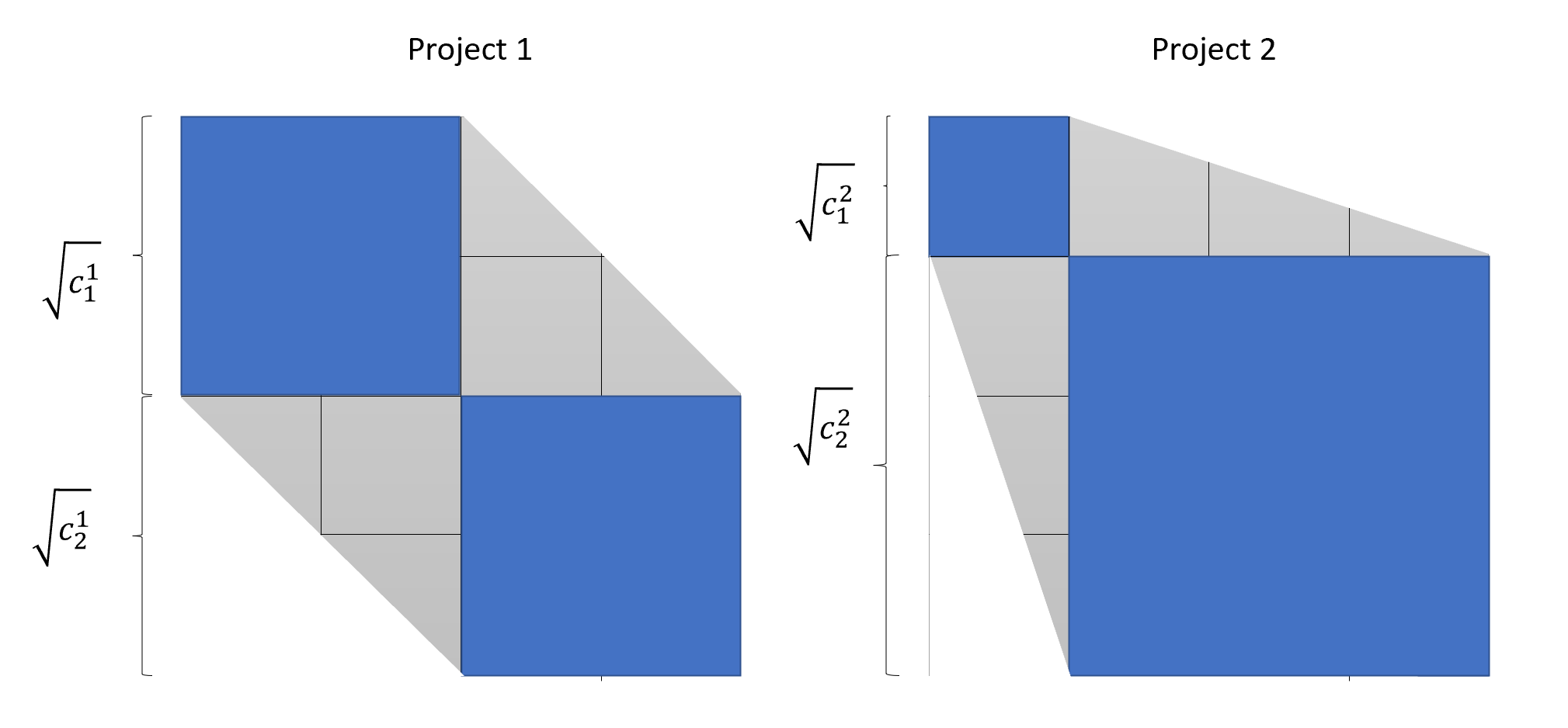
Figure 4: Two projects with equal QF funding targets, and available matching funds covering half of total required matching funds

2.1 Conditional efficiency of the decentralized allocation

Here we revise some of the properties of the decentralized allocation resulting from the mechanism. We start by reproducing BHW’s result which shows that the mechanism achieves a socially efficient allocation (i.e., an allocation that maximizes social welfare), in the case the pool of funds is big enough to satisfy QF matching requirements. Since, as we discussed, this is a demanding scenario, we explore the efficiency of the allocation of limited funds.

As in Buterin, Hitzig, and Weyl (2019), let $V_{i}(F^{p})$ be the currency-equivalent utility a citizen $i$ receives if the funding level of public good $p$ is $F^{p}$. Utilities from different public goods are assumed to be independent, and it is assumed a setting of complete information.

Observation 2.1.

The QF with limited matching mechanism tends to a generate a socially optimal allocation as matching funds tend to be enough to cover target requirements.

The problem that defines the optimal individual contribution from the perspective of backer $i$ is

$$\max_{\{c_{i}\}}V_{i}\bigg{(}\frac{1}{k}(\sum_{i}\sqrt{c_{i}})^{2}+(1-\frac{1}{k})C^{p}\bigg{)}-c_{i}$$

Where we have substituted Equation 5. This problem has a First Order Condition (F.O.C.) given by:

$$V_{i}^{\prime}(F^{p})(\frac{1}{k}\frac{\sum_{i}\sqrt{c_{i}}}{\sqrt{c_{i}}}+(1-\frac{1}{k}))=1$$ (6)

Notice that if $k\xrightarrow{}1$ (i.e., $\sum_{p}M^{p,\text{QF}}\xrightarrow{}D$) then the F.O.C. condition converges to:

$$V_{i}^{\prime}(F^{p})=\frac{\sqrt{c_{i}}}{\sum_{i}\sqrt{c_{i}}}$$ (7)

Summing Equation 7 across individuals gives the socially optimal condition:

$$\sum_{i}V_{i}^{\prime}(F^{p})=1$$

In other words, the marginal cost of investing 1 unit of contribution equals the aggregate marginal benefit for the community. This is the standard efficient condition that a centralized planner would follow to maximize aggregate welfare at cost $c$. Indeed, in the case $k\xrightarrow{}1$ the mechanism converges to the QF mechanism discussed in Section 1.

Also notice that if $k\xrightarrow{}+\infty$ (i.e., $\frac{\sum_{p}M^{p,\text{QF}}}{D}\xrightarrow{}+\infty$) , the F.O.C is

$$V_{i}^{\prime}(C^{P})=1$$

Which is the socially inefficient, private condition.

It follows that enough funds to guarantee the QF matching requirements should be in place in order to sustain full efficiency.

Notice that if we additionally consider the requirements on the pool of matching funds discussed in the previous section, the mechanism will not obtain social efficiency in most practical applications.

2.2 Efficiency in terms of the allocation of limited funds

A related question is into what extent the QF mechanism provides an efficient solution to the problem of allocating a limited pool of matching funds. First, it is useful to recall what would be such condition in the first place. A social planner with limited funds $D$ would maximize the aggregate welfare subject to the financing constraint as follows:

$$\begin{split}\max_{\{F^{p}\}^{p\in P}}\sum_{i}\sum_{p}V^{p}_{i}(F^{p})\\ \textrm{s.t.}\sum_{p}F^{p}=D\end{split}$$

Notice that the F.O.C. for each project $p$ are

$$\sum_{i}V^{\prime p}_{i}(F^{p})-\lambda=0\;\;\;\forall p$$

As result, an socially optimal allocation of limited funds would equalize the sum of marginal utilities across projects.

$$\sum_{i}V^{\prime p}_{i}(F^{p})=\sum_{i}V^{\prime p^{\prime}}_{i}(F^{p^{\prime}}),\ \forall p,p^{\prime}$$

To examine the extent in which the the CQF equalizes marginal benefits across projects, we rearrange Equation 6 and sum across individuals to obtain

$$\sum_{i}V_{i}^{\prime}(F_{p})=\sum_{i}(\frac{1}{k}\frac{\sum_{i}\sqrt{c_{i}}}{\sqrt{c_{i}}}+(1-\frac{1}{k}))^{-1}\;\;\;\forall p$$ (8)

Observation 2.2.

In general, the CQF mechanism does not equalize marginal social benefits of limited matching funds across projects.

Define the RHS of Equation 8 as

$$\lambda_{p}\equiv\sum_{i}(\frac{1}{k}\frac{\sum_{i}\sqrt{c_{i}}}{\sqrt{c_{i}}}+(1-\frac{1}{k}))^{-1}$$

Then, one dimension of the relative inefficiency of the mechanism allocation is given by the variability of this multiplier across projects. Notice, in addition, that this magnitude is observable, and we will explore its empirical behavior in Section 4.3.

To understand the sums of the marginal valuations can vary between projects, it is useful to note, first, that for given availability of matching funds $k$, and number of contributors ($N$), $\lambda_{p}$ will be higher for more equally invested projects.

Proposition 2.3.

Given a value of matching requirements to available funds ($k$), and number of contributors ($N$), the multiplier $\lambda_{p}$ is lower bounded by

$$\lambda_{p}\geq\frac{n^{2}}{\frac{1}{k}\sum_{i}\frac{1}{\alpha_{i}^{p}}+n(1-\frac{1}{k})}$$

which increases with more concentrated contributed projects. This implies that more equally contributed projects face a higher value of the multiplier $\lambda_{p}$.

The proof is in the Appendix.

Second, note that $\lambda_{p}$ is an increasing and concave function with respect to $k$. The fact that the functional form is concave makes the marginal penalty in terms of efficiency relatively higher for low values of $k$. This implies that the level of the relative inefficiency will also be affected by this factor.

Finally, note that $\lambda_{p}\xrightarrow{}N$ (i.e., the marginal social cost under a private allocation) as $k$ increases (i.e., as fewer matching funds are available). In line with what was shown above, this implies that as there are fewer matching funds, the mechanism will converge to the (socially inefficient) private cost. It also implies with more contributors (as $N$ increases) there is a larger space for differences in multipliers across projects .

To further illustrate how the sums of the marginal valuations can vary between projects, consider Figure 5, which illustrates the behavior of $\lambda_{p}$ for three projects that have the same amount of target quadratic funding (i.e., $F^{1,\text{QF}}=F^{2,\text{QF}}=F^{3,\text{QF}}$), and only two contributors ($N=2$). Contributions for Projects 1 and 2 correspond to those illustrated in Figure 4 (i.e., In Project 1, both contributors contribute the same amount, and in Project 2, one contributor contributes twice as much as the second.) In Project 3 one of the contributors contributes 15 times the contribution of the second. The figure shows how $\lambda_{p}$ evolves as $k$ increases for each project (i.e., less available matching funds in relation to target required funds). The figure illustrates how more equally invested projects tend to converge to the inefficient marginal cost faster in terms of relative funding availability.

Figure 5: Simulation of multiplier $\lambda_{p}$ for three projects as $k$ increases. Each project have the same amount of target quadratic funding (i.e., $F^{1,\text{QF}}=F^{2,\text{QF}}=F^{3,\text{QF}}$, and only two contributors. Project 1 is equally contributed by both contributors. In Project 2 one contributor allocates twice of funds that the other. In Project 3, one contributor allocates 15 times more funds than the other.

We can conclude that the allocation of a limited pool of matching funds deviates more from a social optimal allocation: i) the lesser the amount of funds in the pool relatively to total QF target matching fund requirements, ii) the greater the variability in the contribution patterns across projects (i.e., variability in terms of how concentrated or equally invested the projects are), and iii) the higher the number of contributors.

3 Collusion and reciprocal backing

QF has collusion and identity fraud as central vulnerabilities (BHW). While fraud refers to the idea of a participant misrepresenting itself as many (a.k.a., Sybil attack), collusion might take various forms, including agreements between contributors or with other agents outside the mechanism. In this section we focus on problems of the latter type, particularly in incentives for strategic behavior.

Consider two contributors that have candidate projects in the mechanism, and that decide to invest in each other. We might call such a situation “reciprocal backing”. This behavior is interesting because it’s a form of reciprocity, that has been observed in many settings (Fehr and Gächter 2000; Göbel, Vogel, and Weber 2013). We note that such situation could arise from an explicit collusive agreement, or from an implicit behavior. To analyze the economic incentives, we will analyze the cases in which contributors could increase their own payoffs by investing a share of their funds in each other instead of fully backing their own projects. Assume that each contributor has an amount $c$ to invest, and there are no limits for matching funds. Consider the strategy of investing half of the funds in the project of another contributor with the expectation of being invested back. In such a situation the strategic decision takes the form of 2 by 2 simultaneous game, with the following net payoff matrix.

	Invest	Do not invest
Invest	$c$,$c$	$-\frac{c}{2}$,$c\frac{(1+2\sqrt{2})}{2}$
Do not invest	$c\frac{(1+2\sqrt{2})}{2}$,$-\frac{c}{2}$	$0$,$0$

Where, for instance, the upper-left Invest-Invest payoff is given by

$\big{(}2\sqrt{\frac{c}{2}}\big{)}^{2}-c=c$.

The resulting game is a standard Prisoners’ Dilemma, with a non-collusion Nash equilibrium (”Do not invest”, ”Do not invest”).

This example illustrates, as pointed out by BHW, that the collusion problem is mitigated because of unilateral incentives to deviate from the collusive agreement.

A first point to note, however, is that in the practice of QF, rounds might take a repetitive form. For instance, in Gitcoin Grants, projects can participate in every round that take place every two or three months. By December 2020, eight rounds were already closed, and Gitcoin planned to continue organizing rounds, since its aim is to provide a sustained flow of financing for projects. If the strategic game presented above is played infinite times, or if there is uncertainty when it will stop, a collusion can be sustained as a Nash equilibrium, using trigger strategies, or threads (Friedman 1971). This leads to the following proposition:

Proposition 3.1.

Incentives for strategic behavior, taking the form of multilateral reciprocal contributions, are part of a Nash equilibrium when players can participate in a indefinite number of rounds.

See the proof in the Appendix.

When the number of participants in this type of collusion increases above two, the collusion strategy is still profitable when a percentage of the participants deviate. In the no-funding limits case, for example, a collusion strategy with $n$ participants is still profitable under deviation if a percentage of $\alpha^{*}$ still colludes, where

$$\alpha^{*}>\frac{1}{\sqrt{n}}$$ (9)

So, for instance, a reciprocal contribution strategy with 25 investments is profitable if 20% of invests back.

A more realistic scenario is when there is a limited pool of matching funds. Under restrictive funds ($k>1$), collusion incentives are reduced as the pool of funds dry up (BHW). But note this does not happen as fast as one could expect. The following proposition illustrates this observation:

Proposition 3.2.

Under restrictive funds a collusion strategy with $n$ participants is profitable under deviation if a percentage of $\alpha^{**}$ still colludes where

$$\alpha^{**}>\frac{k\bigg{(}(1-\frac{1}{k})+\sqrt{(1-\frac{1}{k})^{2}+4(\frac{n}{k})}\bigg{)}}{2n}$$ (10)

Following the previous example, a reciprocal investment strategy with 25 investments and, for example, (k=20), is profitable if 60% of contributors invests back. As we will confirm in the empirical section below, values of (k) between 10 a 20 are in line with what is taking place in Gitcoin rounds. Figure 6 illustrates further the result in Equation 10. It depicts two cases of collusions sized $n=10$ and $n=25$ respectively, and shows the required percentage of participants for the reciprocal strategy to be profitable, against different levels of (k). The figure serves to illustrate that there are feasible percentages of participation rates in reciprocal strategies that can serve to sustain an equilibrium.

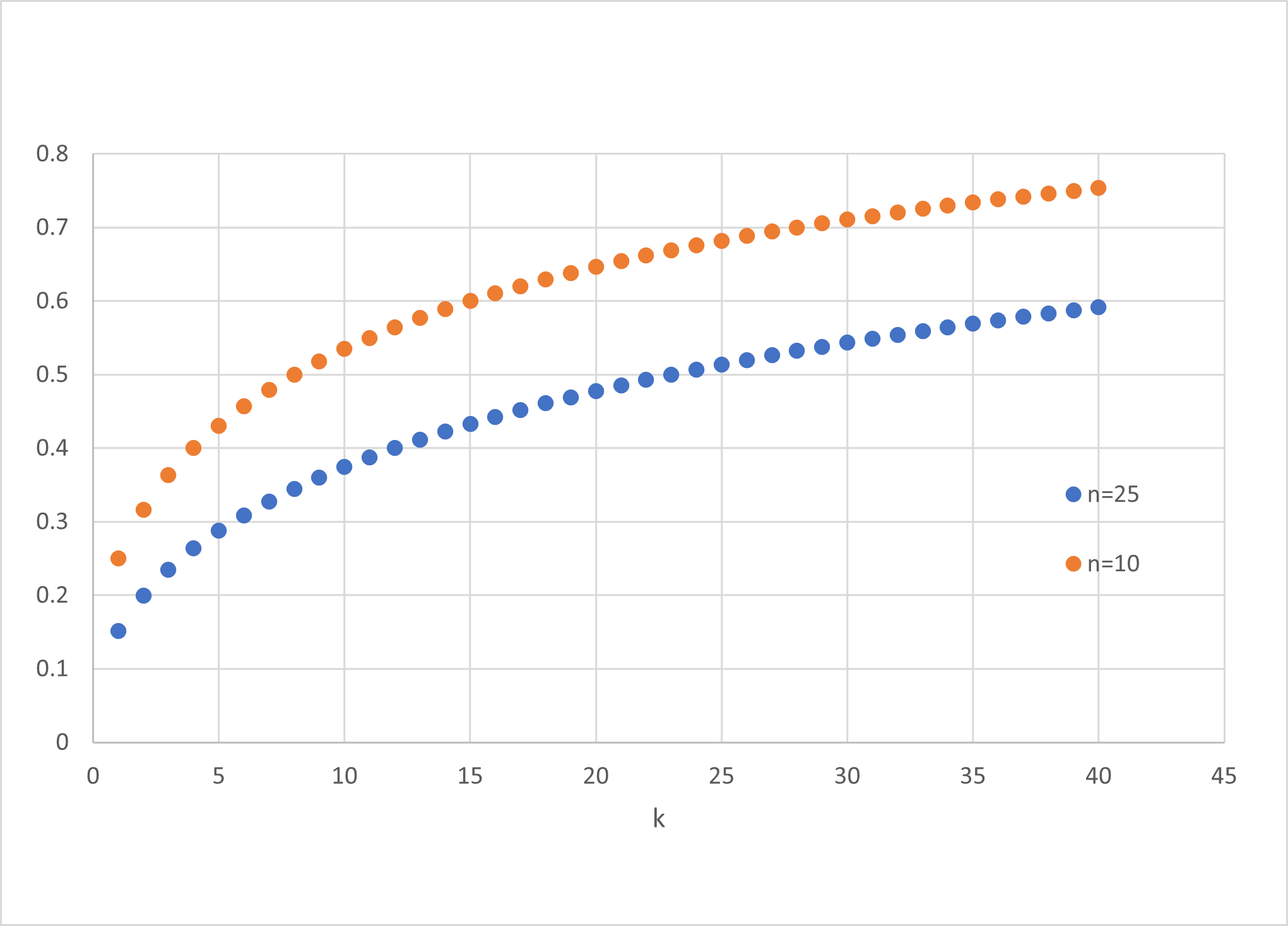
Figure 6: Minimum percentage or participants non deviating for collusion to be profitable

A final point to note is that, in reciprocal contributions taking place in practice, not all participants are subject to the same budget constraint. As we will note in the case of Gitcoin, because rounds for different categories take place simultaneously, each with its own budget constraint, colluding projects do not compete for funding if they are part of different categories. This simple observation leads to the following proposition:

Observation 3.3.

Incentives for strategic behavior in the form of reciprocal investments are higher across project categories than within categories.

4 QF evidence from Gitcoin Grants

4.1 Details of Gitcoin Grants’ 7th and 8th rounds

The 7th Gitcoin Grants round took place between September 15th and October 2nd, 2020. The 8th round took place between the 2nd and 17th of December 2020. The 7th round was organized around three main categories: Infra Tech, Applications (DApps) Tech, and Community Projects. A fourth specific category, Matic Network (technology infrastructure used for scalability) started at the same time. The first three categories received initially a matching endowment of 120 thousand DAI (as we will explain below, on September 23th, the pool of funds increased to 150 thousand DAI each). The Matic endowment received 50 thousand DAI.

The 8th Gitcoin Grants Round presented the same main three categories (DApps, Infra and Community), each endowed with 100 thousand DAI, and three additional categories: Filecoin Liftoff (projects related to Filecoin, the decentralized storage network) with 100 thousand DAI, Apollo (also an initiative related to Filecoin) with 50 thousand DAI, and East-Asia (an initiative to support projects from East-Asia) with 50 thousand DAI.

During the days of a round, contributors could easily find the participating projects by browsing Gitcoin Grants’ webpage, choose which projects to invest in and commit a cryptocurrency transfer. The page reports the total amount received so far by each project, and importantly, provides an estimation of the expected amount to be received by the project in terms of matching funds if an individual contributes (See Figure 7). For this, the website continuously computes the specific allocations taking into account the budget constraint, in line with the discussion above.

Figure 7: Gitcoin Grants webpage extract

4.2 Projects, contributors and amounts

Table 1 displays descriptive statistics on the number of projects, contributors, and total individual contributed amounts per project and category. A total of 249 projects and 1,234 contributors participated in Round 7. The category with the highest number of contributors was DApps Technology with 93 projects (37% of total projects) and 1105 contributors (90% of the contributors). The second most important category in terms of contributors was Community with 82 projects (33%) and 677 contributors (54%). Infra tech displayed less projects (52, 33%), but a similar number of contributors (613, 49%). Finally, the smallest category was Matic, with 19 projects and 190 contributors. Notice that the sum of contributors percentages exceeding 100%, shows that contributors tend to invest in many projects. Round 8 counted with more projects (444) and contributors (4,953), and presented a similar pattern in terms of importance of the main categories (DApps, Community and Infra). Statistics for Round 8 are available in Table 7 in the Appendix.

Table 1: Gitcoin Round 7 Descriptive Statistics

	N	Mean	Std. dev.	Std. error	Median
All categories. projects: 249, contributors: 1234
$c_{i}$	8450	24.895	161.778	1.76	4.75
$\sqrt{c_{i}}$	8450	2.829	4.112	0.04	2.179
Dapp Tech category. projects: 93, contributors: 1105
$c_{i}$	3802	19.407	120.596	1.956	3.64
$\sqrt{c_{i}}$	3798	2.466	3.654	0.059	1.908
Infra Tech category. projects: 56, contributors: 613
$c_{i}$	2220	39.301	247.737	5.258	4.75
$\sqrt{c_{i}}$	2220	3.370	5.287	0.112	2.179
Community category. projects: 82, contributors: 677
$c_{i}$	2142	21.366	115.481	2.495	4.75
$\sqrt{c_{i}}$	2142	2.958	3.553	0.077	2.179
Matic category. projects: 19, contributors: 190
$c_{i}$	345	10.613	39.070	2.103	3.3
$\sqrt{c_{i}}$	345	2.401	2.205	0.119	1.817

Note: This table reports summary statistics on backer contributions per project.

Individual contributions per project $(c_{i}^{p}$) average about 25 DAI (Table 1) in Round 7 and about 30 DAI in Round 8, but these figures can be quite misleading given the fact that the distributions of contributions are severely right-skewed, with 80% of contributions below 10 DAI, 17% between 10 and 100 DAI, and only 3% above 100 DAI in Round 7.

Histograms in Figures 8 (for Round 7), 16 and 17 (for Round 8) in the Appendix reflect this fact. The figures display histograms of total individual contributions per projects by categories, where the range was split in 3 intervals to more accurately visualize the respective frequencies. The graphs show that for all categories contributions are concentrated in values less than 10 DAI.

This pattern of small contributions are notably lower than what has been documented in other crowdfunding settings. For instance, according to Mollick (2014), contributions per backer in Kickstarter for technology projects averaged 73 USD.

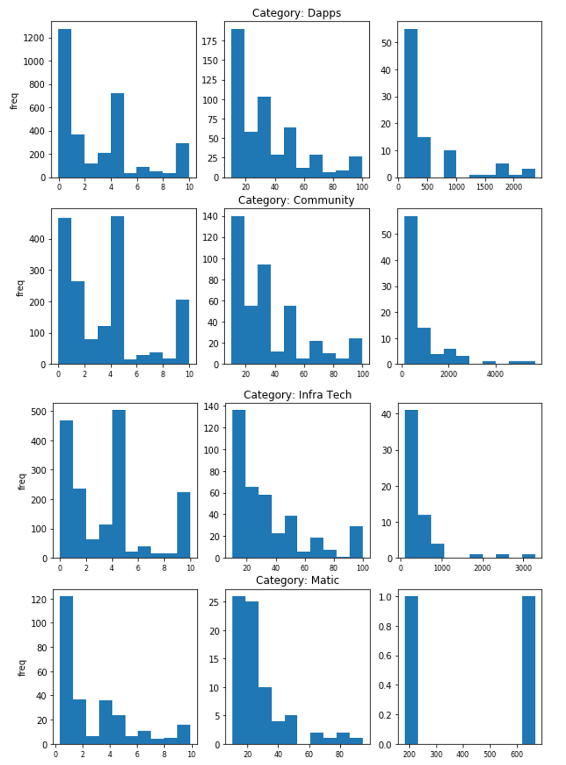
Figure 8: Split range histograms of total individual contributions to projects $c_{i}^{p}$ by category. Round 7

Total contributions per individual and projects invested

In terms of the total contributions per backer (a proxy of $m_{i}$) the median was 20.57 DAI and the mean 170.55 DAI also presenting an asymmetric distribution (Figure 9). In the case of Round 7, for example, nearly 32% of individuals contributed less than a total of 10 DAI, 50% contributed between 10 and 100 DAI, 15% of individuals contributed between 100 and 1,000 DAI, and only 2% contributed above 1,000 DAI.

This pattern of small investments is also consistent with the average number of contributions per backer climbing to 6.85 on average, and a median of 3 contributions. This is also a highly asymmetric distribution as shown in Figure 10 which shows there is an economic significant number of contributors investing in many projects, with 20% investing above 10 projects, and 6% investing above 20.

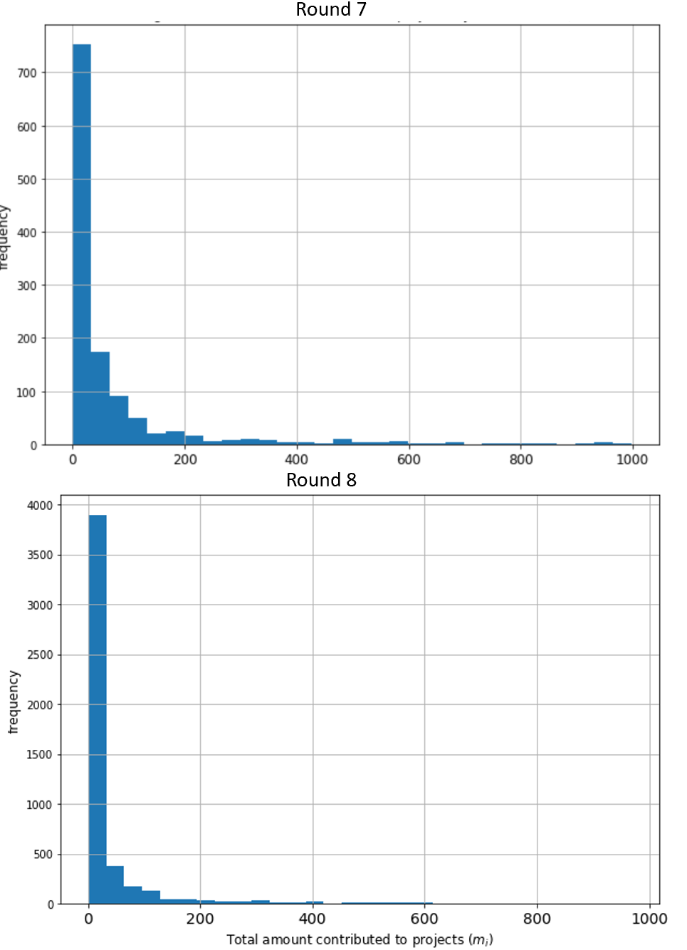
Figure 9: Histograms for the total amount contributed to projects by individuals ($m_{i}$). Rounds 7 and 8

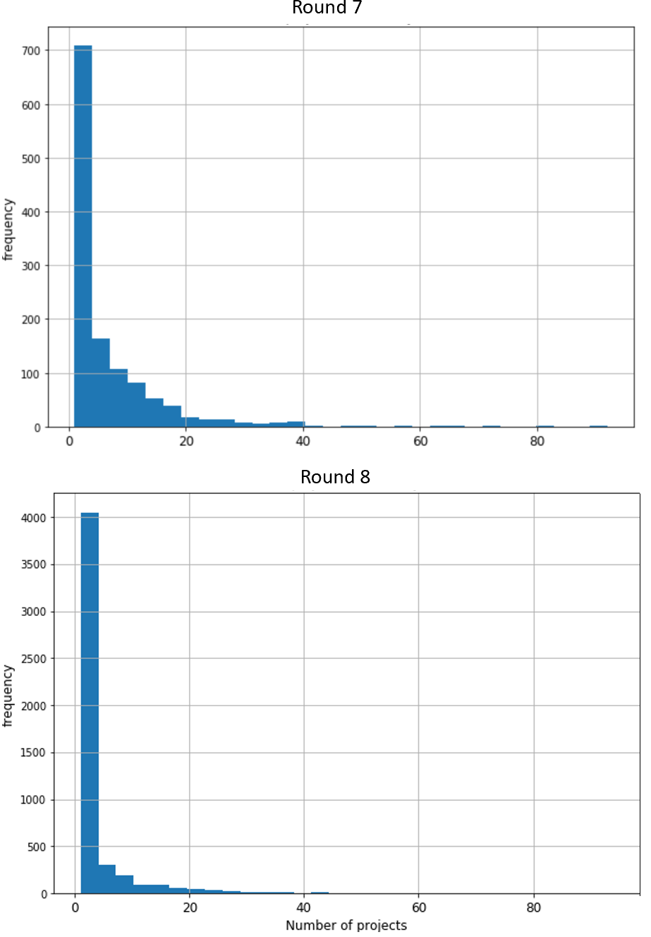
Figure 10: Histograms for the number of projects contributed by individual contributors. Rounds 7 and 8

4.3 Evolution of matching fund requirements to available matching funds ($k$), projects deficits and measured efficiency

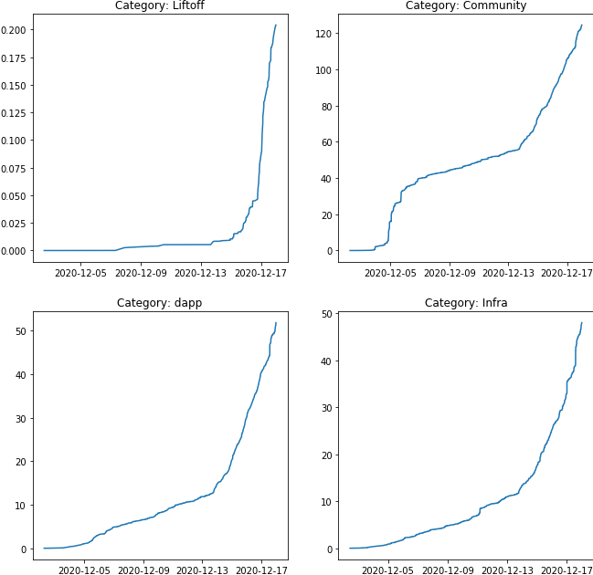
Figure 14: Evolution of budget scale constant $k$ during round8

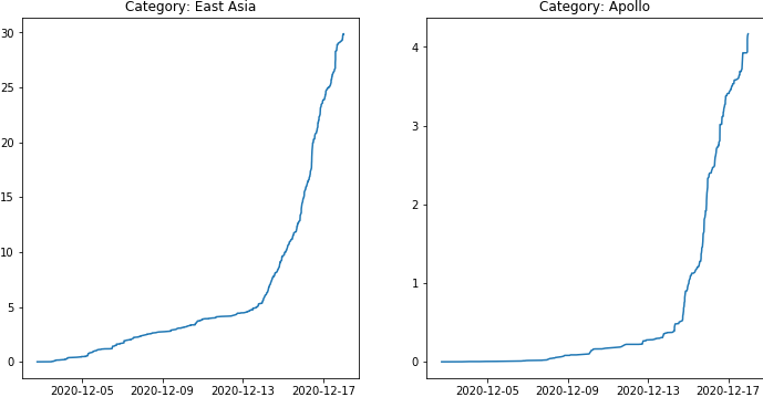
Figure 15: Evolution of budget scale constant $k$ during round 8

The evolution of the constant $k$ (See Equation 3) during the round reflects how quickly required matching funds escalate. Figure 11 plots the constraint for each of the categories in Round 7. Figures 14 and 15 (in the Appendix) provide the plots for categories in Round 8. These figures show that $k$ increased non linearly in all categories, reaching, for example, a value close to 20 for DApps and Infra Tech categories, and close to 12 for the Community category in Round 7. In Round 8, $k$ reached even higher values, approaching 50 for DApps and Infra, and 120 for the Community category. This is not surprising given the fact that the pool of funds for these categories was smaller in Round 8, and the number of individuals contributing nearly quadrupled.

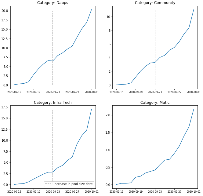
Figure 11: Evolution of matching fund requirements to available matching funds ratio ($k$)

A different behavior resulted in the specific categories. Although these categories do also show a rapid nonlinear increase in the value of $k$, because of the lower number of supporters, they ended with lower $k$ values. For instance, Matic in the 7th round ended with a value of $k$ close to 2, Apollo in round 8 ended with $k$ about 4, and Liftoff ended with a value close to 0.2.

For graphs in Figure 11, the vertical dotted line in the graphs indicates the day the pool of matching funds increased -recall as explained above total funding increased in 25%-. We can see that the effect on $k$ is a slight drop, which quickly resumes growth due to the increase in the quadratic fund target. We will return to this point in the next section.

In terms of the determinants of $k$ , Figure 12 is also illustrative, showing the total matching requirements per project versus the number of contributors. We can identify the relationship proposed by Equation 1 above, where the behavior increases quadratically. This relationship is confirmed in both rounds.

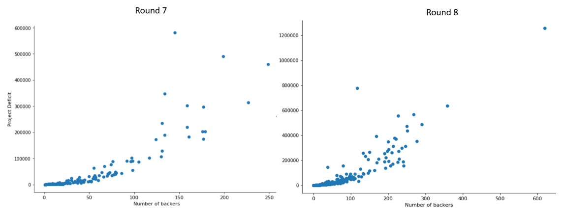
Figure 12: Matching requirements and number of contributors at the end of the round. Rounds 7 and 8

Finally, Table 2 presents summary statistics on $\hat{\lambda_{p}}$. According to Equation 8, a condition for the efficient allocation of limited funds is that the sum of marginal benefits equalizes across projects. Therefore, the standard deviation of $\hat{\lambda_{p}}$ in Table 2 provide a measure of relative inefficiency in the allocation.

Table 2 provides evidence that confirms the theoretical predictions. In first place, categories with relatively more funds available (i.e., a lower final $k$ value), such the specific categories Matic -Round 7-, East Asia and Liftoff -Round 8-, are the categories with less variability in $\lambda_{p}$ across projects. All categories in round 8 resulted in higher variability than those in round 7. We also confirm that the higher the number of participants, the higher the variability in $\hat{\lambda_{p}}$, and lower efficiency in the Round.

Table 2: $\hat{\lambda_{p}}$ allocation efficiency indicator

Category	Projects	Mean	Std. Dev.
Dapp - Round 7	57	10.6060	4.6709
Community - Round 7	53	5.8891	2.6123
Infra - Round 7	36	10.1602	3.2982
Matic - Round 7	19	1.9273	0.1055
Community - Round 8	133	25.1127	21.2072
Dapp - Round 8	114	16.6023	11.7582
Infra - Round 8	43	22.8302	10.3061
East-Asia - Round 8	23	14.7344	5.3482
Liftoff - Round 8	3	0.2325	0.0793

4.4 Reciprocal backing

In Section 3, we discussed that under certain conditions, QF provides incentives for strategic contributions in the form of reciprocal backing. Figure 13 and Table 3 provide evidence on the extent of such behavior.

To measure recyprocal backing we exploit information on the identity of projects’ team members as registered in Gitcoin. Precisely, we define contributions as reciprocal if team members of a project receiving contributions, support back the projects of their contributors. Figure 13 illustrates the measure. On the left panel, the figure plots each project number of reciprocal contributions against the total number of contributed projects (i.e., total outdegree in networks terminology). The total number of contributed projects is similarly constructed, by aggregating all contributions by the project’s team members. A linear approximation to this relationship retrieves a slope of 0.2, suggesting that approximately 20% of the contributions are received back. The measure depicted in the right panel is further restricted to contributions across projects that belong to different categories. Proposition 3.3 above, argued that reciprocal backing incentives were stronger across categories. Here the figure suggests that a contribution in an additional project is related with a probability of reciprocity of 23%. So, while the data confirms the cross-category hypothesis, it also suggests that the magnitude of these incentives are low.

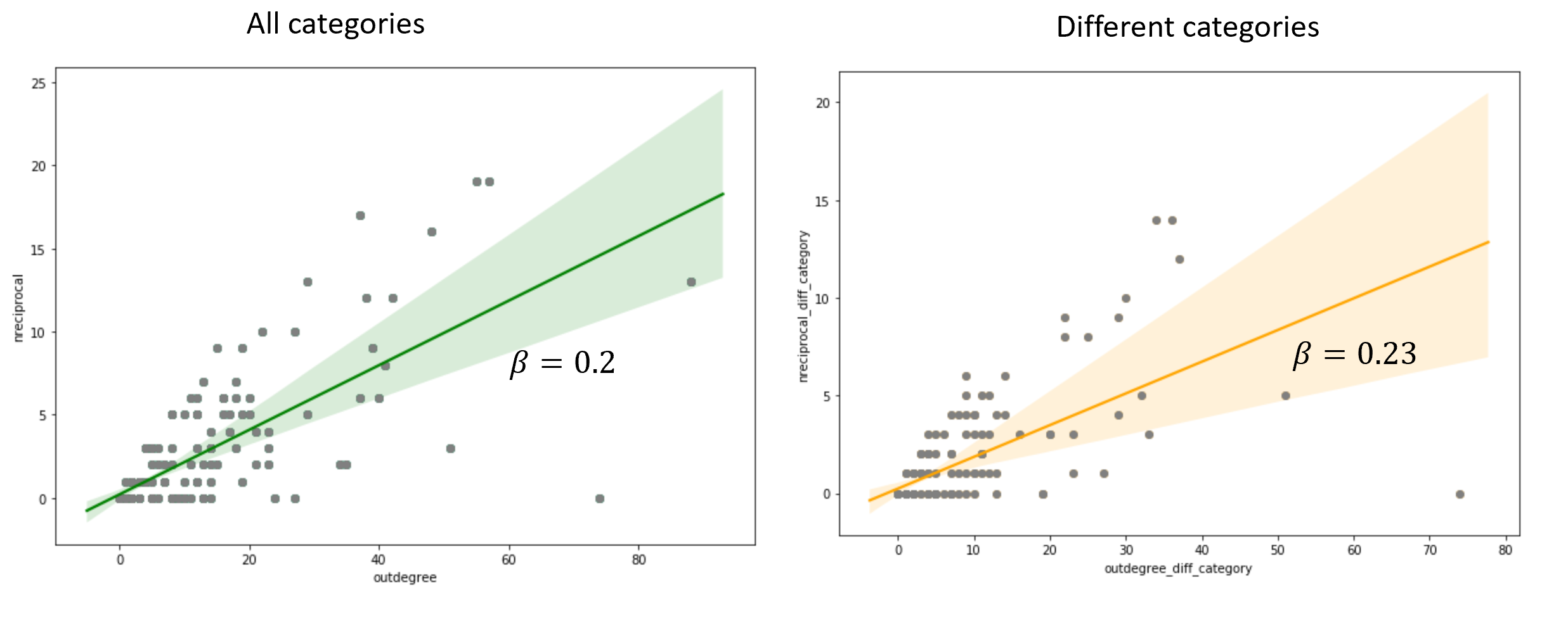
Figure 13: Reciprocal contributions as function of total contributions

We can further examine reciprocal investments across categories in Table 3. Here we consider reciprocal contributions taking into account the relative importance of the respective categories. Column I displays the number of projects for each category as percentage of the total number of projects in the Round. Column II displays the complement of this percentage (i.e. projects that are not in the same category). If contributions were made with independence of the project category, the percentage of reciprocal investments across categories would tend to equal the percentage of projects in Column II. In other words, if reciprocal backing incentives were greater across categories, the resulting percentages would be greater than those in Column II. We confirm this hypothesis in only one of the main three categories. Projects in the Community category, tend to have 71% of their reciprocal contributions in other categories, while only 66% of projects are not in the Community category. This behavior, however, is reverted in the DApp category (55% of reciprocal contributions in other categories against 66% of projects in other categories), and no significant differences appear in the Infra Tech category.

Overall, we conclude that reciprocal backing is present in the data but to a small extent (not explaining more than 20% of investments), and that incentives for reciprocal investments across categories are also small.

Table 3: Reciprocal backing.

Category	Number of projects %	Number of projects- complement %	Reciprocal investments in other categories %
Community	33.49	66.51	71.30
Dapp Tech	33.49	66.51	55.55
Infra Tech	22.64	77.36	76.00
Matic	8.96	91.04	20.51

4.5 Individual contributions and availability of matching funds

Limited availability of matching funds, as explained in Section 2, implies that contributors will reduce their contributions as they learn there are less matching funds available. In this section we examine the relationship between contributions and the availability of matching funds (as measured by the ratio $k$).

First, we will assume that individuals do not anticipate the level of $k$ at the closure of the round and adjust their contributions as information on $k$ is updated (i.e., as the round progresses). As required matching funds increase continuously during the round, we hypothesize that contributions will decrease steadily as $k$ increases.

Second, we will additionally examine an event where the pool of matching funds (exogenously) changed during the round. As a general case, at the beginning of a round, Gitcoin Grants announces the total pool of matching funds for the entire round. However, on one occasion (due to the unexpected entry of philanthropic contributors), on September 23th, 2020, Gitcoin Grants announced an (unexpected) increase in the size of the pool as the round unfolded [^reason]. In this particular event, total matching funds were increased by 25% (from 120 to 150 thousand DAI) for the three main categories (Dapps, Infrastructure and Community). The forth contemporaneous category (Matic) remained unchanged.

In general, an increase in matching funds is expected to stimulate increases in backers’ contributions. However, as noted in Section 4.3, once the round has progressed, requirements on funds to be matched might be already high so that increases in the pool of funds could result in insignificant changes in the corresponding value of $k$. As a result, even considerable increases in the pool of matching funds could result in no incentives to increase backers contributions.

4.5.1 Econometric specifications

To analyze the relationship between contributions and the level of $k$ during the round, we propose a simple econometric model of the form:

$$\sqrt{c_{i,p,t}}=\beta_{0}+\beta_{1}k_{t,\kappa}+\delta_{p}+\epsilon_{i,p}$$

Where $k_{t,\kappa}$ is the constant balancing constraint as defined in Equation 3. The subscript $t$ acknowledges that $k$ changes in time (as the round progresses), and $\kappa$ recognizes that $k$ is specific to the project category (See description on Gitcoin Rounds in Section 4). $\delta_{p}$ adds a project specific fixed effect, and is introduced in some of the specifications estimated.

Second, to examine the event where the pool of matching funds increased during the 7th round, we propose a model of the form:

$$\sqrt{c_{i,p,t}}=\beta_{0}+\beta_{1}t+\beta_{2}Post_{t}+\beta_{3}Increase_{\kappa}+\beta_{4}Post_{t}*Increase_{\kappa}+\delta_{p}+\epsilon_{i,p}$$ (11)

where $t$ stands for the number of the day in which the round took place, $Post_{t}$ is a dummy that is active on September 23th and after that date, and $Increase_{\kappa}$ is a dummy that is active for the categories that increased funds at the mentioned date (i.e., active for Dapps, Infrastructure and Community, and remains inactive for Matic).

Following the hypothesis that contributors will update the information on $k$ as round progresses, we expect $\beta_{1}$ to capture the negative effect on contributions. We also expect the coefficient on the interaction $Post_{t}*Increased$ ($\beta_{4}$) to identify a differential effect (if any) on contributions after September 23th on the round categories that experienced the matching funds pool increase.

4.5.2 Econometric Results

Table 4 presents the results of the econometric model of individual contributions, where the constant $k$ is included as an explanatory factor. In these specifications we consider the square root level of the contribution as the dependent variable.

Table 4: Effects of $k$ on contributions. Round 7

Dependent: Sqrt(c)	(1)	(2)	(3)
Intercept	2.9098***	1.9893***	2.0299***
	(0.0885)	(0.3983)	(0.3907)
Category Dapp	0.1086	1.0488**	1.1628***
	(0.1027)	(0.4136)	(0.4145)
Category Infra Tech	0.4987***	1.2687***	1.0134**
	(0.1235)	(0.4484)	(0.4507)
Category Matic	-0.6979***	0.8435**	1.1431***
	(0.1205)	(0.4226)	(0.4313)
$k$	-0.0186*	-0.031***	-0.0678***
	(0.0097)	(0.0104)	(0.0235)
$k$*Category Dapp			0.023
			(0.0263)
$k$*Category Infra Tech			0.0737**
			(0.0329)
$k$*Category Matic			-0.4104***
			(0.147)
Project Fixed Effect	No	Yes	Yes
Number of obs.	8650	8650	8650
Adj-R2	0.004	0.031	0.033
F-statistic:	19.005	515.592	8049.32
Prob (F-statistic)	0	0	0

Note: Project level clustered robust standard errors in parenthesis.

Column 1 shows that the relationship with $k$ is negative and statistically significant, and the coefficient remains negative and significant as project fixed effects are included. Column 3 additionally allows the $k$ effect to vary across categories. The results allow calculating that the net effect of $k$ was negative and significant in the Community (baseline, -0.0678), DApps (-0.0678+0.023=-0.04), and Matic (-0.0678-0.4104=-0.4782) categories. The exception is Infrastructure category, where the resulting effect is statistically not different from zero (-0.0678+0.0737=0.0059).

Overall these results seem to confirm the hypothesis that backers update their contributions as they learn on the state of the matching funds constrain (i.e., that new contributions will be matched with lower amounts by the matching fund).

Table 5 and 6 present the results on the regressions that explore the consequences of the increase in funds in the main categories in September 23th. Each table presents variations on the baseline specification in Equation 11. Table 5 includes project fixed effects in Columns 3 and 4, and category-specific linear trends in Columns 2 and 4. Table 6 presents results from reducing the sample of analysis to the immediate dates to the event. Precisely, the sample is restricted to 2 days before and 2 days after the increase (Columns 1 and 2), and to 1 day before and 1 day after the increase (Columns 3 and 4).

Table 5 shows a negative and statistically significant coefficient on $t$, confirming a negative trend in contributions as the round progresses. The coefficients on the interaction $Post_{t}*Increased$, however, show that there are no significant changes associated with the increase in funds event. Consistently, Table 6 shows no sign of effects in the immediacy of the event. $Post$ tends to show negative but insignificant changes. The coefficient on the interaction $Post_{t}*Increased$ is generally low in terms of its standard error and therefore remains statistically insignificant across specifications.

Table 5: Examining the pool of matching funds increase event.

Dependent: Squared root of contribution	(1)	(2)	(3)	(4)
Intercept	1.9569***	2.0231***	1.8298***	1.8745***
	(0.1388)	(0.1497)	(0.0907)	(0.1133)
Category Dapp	0.0223	0.037	1.083***	1.212***
	(0.1347)	(0.3231)	(0.0748)	(0.1966)
Category Infra Tech	0.4735**	-0.0332	1.3742***	0.9291***
	(0.1885)	(0.3815)	(0.0706)	(0.2561)
Category Matic	0.7828***	0.7808***	1.5012***	1.5337***
	(0.2274)	(0.2716)	(0.1579)	(0.2228)
t	-0.0502***	-0.0641***	-0.0685***	-0.0843***
	(0.018)	(0.0221)	(0.0177)	(0.0222)
Post	-0.0703	0.0772	0.096	0.233
	(0.4375)	(0.3605)	(0.4621)	(0.3197)
Increased	1.174***	1.2422***	0.3286***	0.3409***
	(0.1376)	(0.1972)	(0.0749)	(0.1205)
Post*Increased	0.329	0.1774	0.1923	0.0518
	(0.4161)	(0.3854)	(0.4501)	(0.3427)
Project Fixed Effect	No	No	Yes	Yes
Category linear trends	No	Yes	No	Yes
Number of obs.	8650	8650	8650	8650
Adj-R2	0.005	0.006	0.033	0.033
F-statistic:	367.027	269.205	83.347	51.652
Prob (F-statistic)	0	0	0	0

Note: Project level clustered robust standard errors in parenthesis.

Table 6: Examining the pool of matching funds increase event.

Dependent: Squared root of contribution	(1)	(2)	(3)	(4)
Intercept	1.6811***	1.7579***	1.2939***	1.942***
	(0.1205)	(0.1773)	(0.1168)	(0.2)
Category Dapp	0.0471	0.1197	1.6631***	1.14***
	(0.2032)	(0.2991)	(0.077)	(0.1285)
Category Infra Tech	0.5425**	0.1294	2.074***	0.8225***
	(0.2628)	(0.3194)	(0.0573)	(0.071)
Category Matic	0.6343***	0.6205**	1.3915***	2.2013***
	(0.2101)	(0.3005)	(0.2031)	(0.4045)
Post	-0.2649	-0.9059**	0.1015	-1.0707
	(0.5075)	(0.4078)	(0.622)	(0.7055)
Increased	1.0468***	1.1374***	-0.0975	-0.2593
	(0.1553)	(0.2587)	(0.1299)	(0.2349)
Post*Increased	0.0499	0.6756	-0.3232	1.3205*
	(0.514)	(0.4872)	(0.6202)	(0.7242)
Project Fixed Effect	No	No	Yes	Yes
Data window	2 days	2 days	1 day	1 day
Number of obs.	1856	856	1856	856
Adj-R2	0.005	-0.001	0.124	0.332
F-statistic:	201.9	160.929	100.18	290.313
Prob (F-statistic)	0	0	0	0

Note: Project level clustered robust standard errors in parenthesis.

5 Discussion and conclusions

Buterin, Hitzig, and Weyl (2019) (BHW) presents an innovative financing mechanism for public goods with some very promising features. Our interest in this paper has been to explore the matching fund requirements of the mechanism and its implications in terms of efficiency. In practice, as we have exemplified with the case of Gitcoin Grants, the implementation of the QF mechanism will most likely take place in the form of its capital-constrained version (CQF). This is because matching funds requirements increase fast, quadratically in the number of contributors (Proposition 1.2). The evidence also shows that there is a tendency among contributors to make small contributions to multiple projects (Section 4.2), which also increase matching requirements. The tighter the restriction on matching funds, the lower the social efficiency in the BWH sense.

Seeking to increase the matching pool of funds as a response seems difficult in line with the evidence emerging from Gitcoin Grants. The data illustrates that the funding restriction is reached fast, in the first days of the rounds (Section 4.3). Increases in philanthropic funds might only provide a temporary relief, since funds would eventually need to increase 20 to 50 times their size in some cases -as can be observed in the value of $k$ in Section 4.3-. An illustrative example is an event of funds increasing 25% in the middle of Round 7, which had almost negligible effect on the ratio of required funds (to available funds) $k$ (Figures 11 and 14).

As a result, it is expected that projects will compete for the limited pool of matching funds. It follows that a more appropriate question to whether there will be some degree of inefficiency -relative to an otherwise limitless funding scenario-, is the question of to what extent the allocation of limited funds is efficient. Social benefits from available projects should equalize on the margin for such an efficient allocation. (Section 2.2). It turns out that that the CQF allocation entails some deviations from such an allocation. Deviations are expected to be greater the lesser matching funds are available, the higher the differences in patterns of contributions across projects, and the higher the number of contributors. The data from Gitcoin Grants also provides evidence in this respect. We have shown that the mechanism did a better job in equalizing these benefits when there were relatively more matching funds available (Section 4.3).

Other observations emerging from Gitcoin data seem particularly relevant in terms of the implementation of the mechanism. For instance, the fact that a higher correlation in contributions to projects among individuals is related to higher needs of matching funds (Proposition 1.4) implies that features that ease or foster contributions correlations among individuals have implications in terms of funds requirements and efficiency. An example of such feature was implemented during the 7th Gitcoin round. Grants Collections allowed any user to replicate a curated portfolio of contributions from another contributor. While it is beyond the scope of this paper to document the effect of the introduction of such a feature, it is worth noting that such changes have effects that are worthwhile study.

Another important characteristic that emerges from the data analysis of contributions is related to their small relative size (Section 4.2) (i.e., relative to those contributed in other crowdfunding platforms such as Kickstarter). As mentioned above, small contributions accelerates the needs for matching funds. While such behavior could be attributable to the potential of quadratic backing per se (while there are available matching funds funds), we have also noted that this behavior might also be the result of strategic incentives. In particular, contributors with listed projects might seek a return from reciprocity by other contributors (Section 3).

QF has certainly powerful properties, and we expect that there will much more research on how to best implement QF ahead. This research should take into account the economics of fund requirements, such as to how to best allocate limited funds. This will be particularly important in terms of implementing QF in applications associated with large communities. How to discourage strategic behavior is another line of further research.

References

Agrawal, Ajay, Christian Catalini, and Avi Goldfarb. n.d. “Some Simple Economics of Crowdfunding,” 35.

Andreoni, James. 2006. “Leadership Giving in Charitable Fund-Raising.” Journal of Public Economic Theory 8 (1): 1–22. https://doi.org/10.1111/j.1467-9779.2006.00250.x.

August, Terrence, Wei Chen, and Kevin Zhu. 2021. “Competition Among Proprietary and Open-Source Software Firms: The Role of Licensing in Strategic Contribution.” Management Science 67 (5): 3041–66. https://doi.org/10.1287/mnsc.2020.3674.

Baker, Michael, A. Abigail Payne, and Michael Smart. 1999. “An Empirical Study of Matching Grants: The ‘Cap on CAP’.” Journal of Public Economics 72 (2): 269–88. https://doi.org/10.1016/S0047-2727(98)00092-9.

Belleflamme, Paul, Thomas Lambert, and Armin Schwienbacher. 2014. “Crowdfunding: Tapping the Right Crowd.” Journal of Business Venturing 29 (5): 585–609. https://doi.org/10.1016/j.jbusvent.2013.07.003.

Burtch, Gordon, Anindya Ghose, and Sunil Wattal. 2015. “The Hidden Cost of Accommodating Crowdfunder Privacy Preferences: A Randomized Field Experiment.” Management Science 61 (5): 949–62. https://doi.org/10.1287/mnsc.2014.2069.

Buterin, Vitalik. 2019. “Quadratic Payments: A Primer.” https://vitalik.ca/general/2019/12/07/quadratic.html.

Buterin, Vitalik, Zoë Hitzig, and E. Glen Weyl. 2019. “A Flexible Design for Funding Public Goods.” Management Science 65 (11). INFORMS: 5171–87.

Clarke, Edward H. 1971. “Multipart Pricing of Public Goods.” Public Choice 11 (1). Springer: 17–33.

Fehr, Ernst, and Simon Gächter. 2000. “Fairness and Retaliation: The Economics of Reciprocity.” Journal of Economic Perspectives 14 (3): 159–81.

Friedman, James W. 1971. “A Non-Cooperative Equilibrium for Supergames.” The Review of Economic Studies 38 (1). JSTOR: 1–12.

Göbel, Markus, Rick Vogel, and Christiana Weber. 2013. “Management Research on Reciprocity: A Review of the Literature.” Business Research 6 (1). Springer: 34–53.

Groves, Theodore. 1973. “Incentives in Teams.” Econometrica: Journal of the Econometric Society. JSTOR, 617–31.

Groves, Theodore, and John Ledyard. 1977. “Optimal Allocation of Public Goods: A Solution to the” Free Rider” Problem.” Econometrica: Journal of the Econometric Society. JSTOR, 783–809.

Huck, Steffen, and Imran Rasul. 2011. “Matched Fundraising: Evidence from a Natural Field Experiment.” Journal of Public Economics, Charitable giving and fundraising special issue, 95 (5): 351–62. https://doi.org/10.1016/j.jpubeco.2010.10.005.

Hylland, Aanund, and Richard Zeckhauser. 1979. “The Efficient Allocation of Individuals to Positions.” Journal of Political Economy 87 (2). The University of Chicago Press: 293–314.

Lalley, Steven, and E. Glen Weyl. 2019. “Nash Equilibria for Quadratic Voting.” Available at SSRN 2488763.

Meyskens, Moriah, and Lacy Bird. 2015. “Crowdfunding and Value Creation.” Entrepreneurship Research Journal 5 (2). https://doi.org/10.1515/erj-2015-0007.

Mollick, Ethan. 2014. “The Dynamics of Crowdfunding: An Exploratory Study.” Journal of Business Venturing 29 (1). Elsevier: 1–16.

Nagle, Frank. 2019. “Open Source Software and Firm Productivity.” Management Science 65 (3): 1191–1215. https://doi.org/10.1287/mnsc.2017.2977.

Nakasai, Keitaro, Hideaki Hata, Saya Onoue, and Kenichi Matsumoto. 2017. “Analysis of Donations in the Eclipse Project.” In 2017 8th International Workshop on Empirical Software Engineering in Practice (IWESEP), 18–22. Tokyo, Japan: IEEE. https://doi.org/10.1109/IWESEP.2017.19.

Overney, Cassandra, Jens Meinicke, Christian Kästner, and Bogdan Vasilescu. 2020. “How to Not Get Rich: An Empirical Study of Donations in Open Source.” In Proceedings of the ACM/IEEE 42nd International Conference on Software Engineering, 1209–21. Seoul South Korea: ACM. https://doi.org/10.1145/3377811.3380410.

Samuelson, Paul A. 1954. “The Pure Theory of Public Expenditure.” The Review of Economics and Statistics, 387–89.

Short, Jeremy C., David J. Ketchen, Aaron F. McKenny, Thomas H. Allison, and R. Duane Ireland. 2017. “Research on Crowdfunding: Reviewing the (Very Recent) Past and Celebrating the Present.” Entrepreneurship Theory and Practice 41 (2): 149–60. https://doi.org/10.1111/etap.12270.

Vickrey, William. 1961. “Counterspeculation, Auctions, and Competitive Sealed Tenders.” The Journal of Finance 16 (1). JSTOR: 8–37.

von Krogh, Georg, and Eric von Hippel. 2006. “The Promise of Research on Open Source Software.” Management Science 52 (7): 975–83. https://doi.org/10.1287/mnsc.1060.0560.

Weyl, E. Glen. 2012. “Quadratic Vote Buying.” Unpublished, University of Chicago.

Appendix A Proofs

Proof.

Proof of Proposition 1.3

As shown in Equation 1 QF rule requirements can be decomposed into funds contributed by individual contributors and matching fund requirements as follows

$$F^{p,\text{QF}}=(\sum\sqrt{c_{i}})^{2}=\sum(\sqrt{c_{i}})^{2}+2\sum_{i\neq j}\sqrt{c_{i}}\sqrt{c_{j}}$$

Dividing each side by $F^{p,\text{QF}}$

$$1=\sum\big{(}\frac{\sqrt{c_{i}}}{\sum\sqrt{c_{i}}}\big{)}^{2}+\frac{2\sum_{i\neq j}\sqrt{c_{i}}\sqrt{c_{j}}}{F^{p,\text{QF}}}$$

Using the definition of $\alpha_{i}$ and solving for $2\sum_{i\neq j}\sqrt{c_{i}}\sqrt{c_{j}}$

$$2\sum_{i\neq j}\sqrt{c_{i}}\sqrt{c_{j}}=(1-\sum\alpha_{i}^{2})F^{p,\text{QF}}$$ (12)

The LHS of the equation are the matching fund requirements. Notice that matching fund requirements are lower the higher is $\sum\alpha_{i}^{2}$. Notice $\sum\alpha_{i}^{2}$ usually used as the Herfindahl-Hirschman HHI concentration index. This quantity can also be expressed in terms of a variability indicator as the sampling variance. Using the sampling variance definition:

$$\sigma^{2}=\frac{1}{n}\sum_{i}(\alpha_{i}-\bar{\alpha})^{2}=\frac{1}{n}\sum_{i}(\alpha_{i}^{2}-2\alpha_{i}\bar{\alpha}+\bar{\alpha}^{2})=\frac{1}{n}\sum_{i}\alpha_{i}^{2}-2n\bar{\alpha}^{2}+n\bar{\alpha}^{2}=\frac{1}{n}\sum_{i}\alpha_{i}^{2}-n\bar{\alpha}^{2}$$

Solving for $\sum\alpha_{i}^{2}$, gives:

$$\sum_{i}\alpha_{i}^{2}=n\sigma^{2}+n\bar{\alpha}^{2}$$

Substituting in Equation 12, gives:

$$2\sum_{i\neq j}\sqrt{c_{i}}\sqrt{c_{j}}=(1-n\sigma^{2}-n\bar{\alpha}^{2})F^{p,\text{QF}}$$

∎

Proof.

Proof of Proposition 1.4

The maximum subsidy results from solving the problem:

$$\max_{s_{i}^{p},i\in I,p\in P}2\sum_{p}\sum_{i\neq j}\sqrt{s_{i}^{p}m_{i}s_{j}^{p}m_{j}}+\sum_{i}\lambda_{i}(1-\sum_{p}s_{i}^{p})$$

And the first order condition with respect to $s_{i}^{p}$ is

$$2\frac{1}{2}{(s_{i}^{p})}^{-\frac{1}{2}}\sqrt{m_{i}s_{j}^{p}m_{j}}=\lambda_{i},\forall i,p$$

Evaluating this condition for two projects $p$ and $p^{\prime}$ and dividing each side of the each equation gives:

$$(\frac{s_{i}^{p}}{s_{i}^{p^{\prime}}})^{-\frac{1}{2}}(\frac{s_{j}^{p}}{s_{j}^{p^{\prime}}})^{\frac{1}{2}}=1$$

Or alternatively:

$$\frac{s_{i}^{p}}{s_{i}^{p^{\prime}}}=\frac{s_{j}^{p}}{s_{j}^{p^{\prime}}}$$

Therefore, the total required subsidy is maximized when the invested shares across individuals are perfectly correlated.

∎

Proof.

Proof of Proposition 2.3

Here we show that, for a given value of $k$ and $n$, $\lambda_{p}$is higher for more equally contributed projects.

Denote $\alpha_{i}=\frac{\sqrt{c_{i}^{p}}}{\sum_{i}\sqrt{c_{i}^{p}}}$ as measure of the share of project $p$ contributed by $i$. We have that

$$\lambda_{p}\equiv\sum_{i}\frac{1}{(\frac{1}{k}\frac{1}{\alpha_{i}^{p}}+(1-\frac{1}{k}))}\geq\frac{n^{2}}{\sum_{i}(\frac{1}{k}\frac{1}{\alpha_{i}^{p}}+(1-\frac{1}{k}))}=\frac{n^{2}}{\frac{1}{k}\sum_{i}\frac{1}{\alpha_{i}^{p}}+n(1-\frac{1}{k})}$$

Where the inequality follows the application of the inequality known Sedrakyan’s inequality, Bergström’s inequality, or Titu’s lemma (i.e., for reals $a_{1},a_{2},...,a_{n}$ and $b_{1},b_{2},...,b_{n},$ we have $\frac{a_{1}^{2}}{b_{1}}+\frac{a_{2}^{2}}{b_{2}}+...+\frac{a_{n}^{2}}{b_{n}}\geq\frac{(a_{1}+a_{2}+...+a_{n})^{2}}{b_{1}+b_{2}+...+b_{n}}$ ). The result is a lower bound for $\lambda_{p}$. Notice that this value increases as projects are more equally invested (less concentrated among contributors). Using Sedrakyan’s inequality, and the fact that $\sum_{i}\alpha_{i}=1$ we also have that $\sum_{i}\frac{1}{\alpha_{i}}\geq n^{2}$ , with $\sum_{i}\frac{1}{\alpha_{i}}=n^{2}$ for the special case in which $\alpha_{i}=\frac{1}{n},\forall i$. Indeed, $\sum_{i}\frac{1}{\alpha_{i}}$ can be viewed as a measure of concentration (i.e., increases as projects are more unequally contributed). This is because $f(x)=\frac{1}{x}$ is a strictly convex function. Therefore more concentrated invested projects imply lower values of $\lambda_{p}$.

∎

Proof.

Proof of Proposition 3.1

The proposition follows the application of the result in friedmanNoncooperativeEquilibriumSupergames1971 in this specific case. As an example, consider the static game presented above, and assume a time discount factor given by the rate $r$. A collusion can be sustained using a trigger strategy, of the type “Invest in the other party project meanwhile the other party invests back. If the other party ceases to invest, do not invest in the other party again.” Note that if both parties collude following this strategy, this gives individuals a constant stream of payoffs $c$ to infinity, with a present value given by: $\sum_{i=0}^{\infty}\frac{c}{(1+r)^{i}}=c+\frac{c}{r}$. If one party deviates and do not invests, the resulting outcome is given by the deviation outcome in the present, plus 0 in the future.(i.e.,: $c(\frac{1+2\sqrt{2}}{2})$). This implies that the collusion will be maintained as long as $c+\frac{c}{r}\geq c(\frac{1+2\sqrt{2}}{2})$, which implies, in this case, that the collusion will be maintained while $r\leq\frac{2}{2\sqrt{2}-1}\approx 1.09=109$. Since it is reasonable to expect $r$ to remain below 109, it follows that in this particular game there are incentives to maintain the collusion indefinitely.
∎

Proof.

Proof of Proposition 3.2

Assuming that only a fraction $\alpha$ of the $n$ individuals contribute $\frac{c}{n}$, the total amount contributed by backers is $\alpha c$ , and the target QF matching to resulting from the mechanism would be $\big{(}\alpha n\sqrt{\frac{c}{n}}\big{)}^{2}$ in the absence of budget limits to the fund. If there are contrains on the pool of matching funds, the actual amounts to be received by the project, as defined in Equation 5 are

$$F^{p}=\frac{1}{k}\bigg{[}\big{(}\alpha n\sqrt{\frac{c}{n}}\big{)}^{2}-\alpha c\bigg{]}+\alpha c=c\bigg{[}\ \frac{1}{k}\big{(}\alpha^{2}n-\alpha\big{)}+\alpha\bigg{]}$$

The return of investing $c$ in this strategy will be positive if $F^{p}-c>0$, or

$$\bigg{[}\ \frac{1}{k}\big{(}\alpha^{2}n-\alpha\big{)}+\alpha\bigg{]}-1>0$$

Which is equalivalent to

$$\frac{n}{k}\alpha^{2}+(1-\frac{1}{k})\alpha-1>0$$

Solving the quadratic equation yields that

$$\alpha^{**}>\frac{k\bigg{(}(1-\frac{1}{k})+\sqrt{(1-\frac{1}{k})^{2}+4(\frac{n}{k})}\bigg{)}}{2n}$$

Note that if $k\xrightarrow{}1$ , then $\alpha^{**}\xrightarrow{}{\frac{1}{\sqrt{n}}}$ , which is Equation 9. Also if , $k\xrightarrow{}+\infty$ then $\alpha^{**}\xrightarrow{}{+\infty}$.

∎

Appendix B Tables and figures

Table 7: Gitcoin Round 8 Descriptive Statistics

Category	Variable	N	Mean	Std. Dev.	Median
All	$c_{i}$	18392	29.632	482.553	4.470
(projects: 444 contributors: 4953)	$\sqrt{c_{i}}$	18392	2.625	4.769	2.114
Dapp	$c_{i}$	6317	19.466	379.871	3.800
(projects: 182 contributors: 2608)	$\sqrt{c_{i}}$	6317	2.385	3.712	1.949
Community	$c_{i}$	7311	37.862	632.955	4.250
(projects: 177 contributors: 2854)	$\sqrt{c_{i}}$	7311	2.697	5.531	2.062
Infra	$c_{i}$	4295	25.742	301.379	4.410
(projects: 55 contributors: 1431)	$\sqrt{c_{i}}$	4295	2.551	4.386	2.100
East-Asia	$c_{i}$	1293	16.619	88.176	3.800
(projects: 38 contributors: 811)	$\sqrt{c_{i}}$	1293	2.662	3.088	1.949
Lift-off	$c_{i}$	137	28.540	245.225	0.998
(projects: 10 contributors: 119)	$\sqrt{c_{i}}$	137	1.874	5.021	0.999
Apollo	$c_{i}$	332	27.908	198.974	2.000
(projects: 20 contributors: 287)	$\sqrt{c_{i}}$	332	2.608	4.601	1.414

Note: This table reports summary statistics on the total backer contributions per project

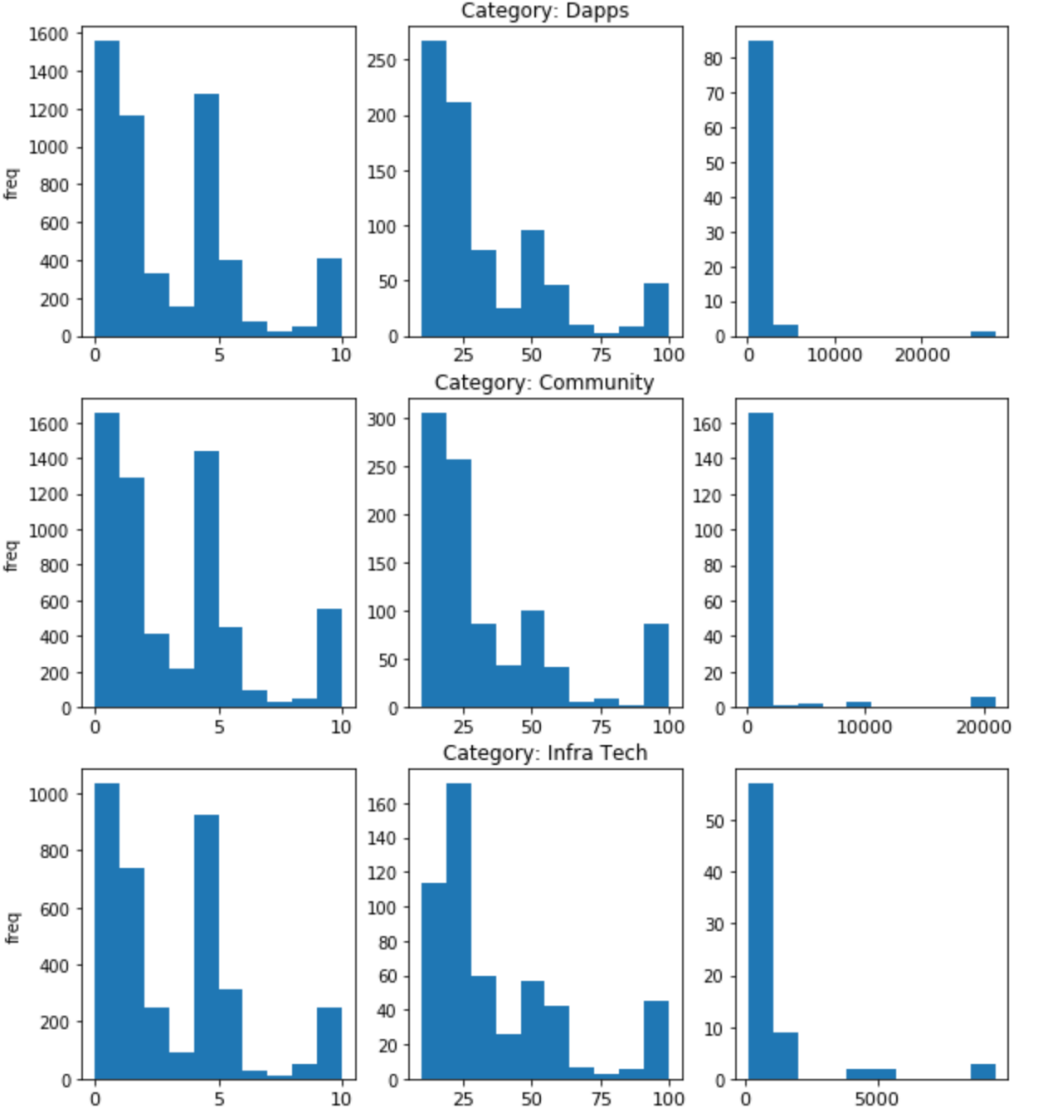
Figure 16: Split range histograms of total individual contributions to projects $c_{i}^{p}$ by category. Round 8

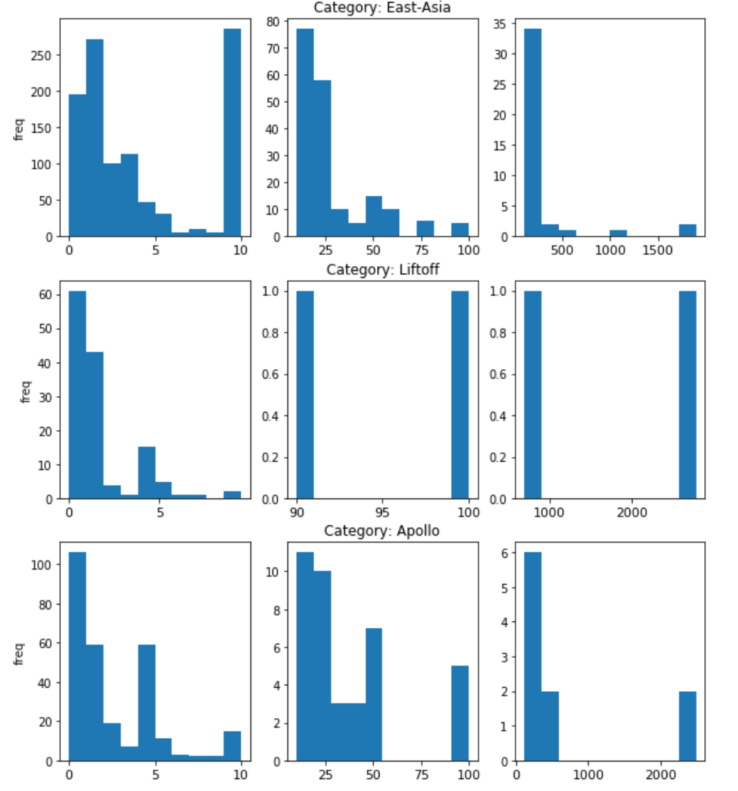
Figure 17: Split range histograms of total individual contributions to projects $c_{i}^{p}$ by category. Round 8