Deep FPF: Gain function approximation in high-dimensional setting

Abstract

In this paper, we present a novel approach to approximate the gain function of the feedback particle filter (FPF). The exact gain function is the solution of a Poisson equation involving a probability-weighted Laplacian. The numerical problem is to approximate the exact gain function using only finitely many particles sampled from the probability distribution.

Inspired by the recent success of the deep learning methods, we represent the gain function as a gradient of the output of a neural network. Thereupon considering a certain variational formulation of the Poisson equation, an optimization problem is posed for learning the weights of the neural network. A stochastic gradient algorithm is described for this purpose.

The proposed approach has two significant properties/advantages: (i) The stochastic optimization algorithm allows one to process, in parallel, only a batch of samples (particles) ensuring good scaling properties with the number of particles; (ii) The remarkable representation power of neural networks means that the algorithm is potentially applicable and useful to solve high-dimensional problems. We numerically establish these two properties and provide extensive comparison to the existing approaches.

I Introduction

This research is motivated by the following questions: What is the principled approach to apply the deep learning methodology to the stochastic filtering problem? Can the well known curse of dimensionality in these problems be mitigated by learning certain geometric structures using neural networks?

In this paper, we present a principled approach to address these questions, based on the use of the feedback particle filter (FPF) methodology. The FPF methodology is applicable to the continuous-time stochastic filtering problem modeled by the following nonlinear stochastic differential equations (sde) [1]:

$$\,\mathrm{d}X_{t} =a(X_{t})dt+\sigma(X_{t})\,\mathrm{d}B_{t},$$ (1a)

$$\,\mathrm{d}Z_{t} =h(X_{t})dt+\,\mathrm{d}W_{t},$$ (1b)

where $X_{t}\in\mathbb{R}^{d}$ is the state of a hidden Markov process at time $t$, $Z_{t}\in\mathbb{R}$ is the observation process, $\{B_{t}\}_{t\geq 0}$ and $\{W_{t}\}_{t\geq 0}$ are two mutually independent Wiener processes, and the functions $a(\cdot)$, $\sigma(\cdot)$, and $h(\cdot)$ are assumed to be continuously differentiable. The objective of the filtering problem is to compute the posterior distribution, i.e., the conditional distribution of $X_{t}$ given the history of observations ${\cal Z}_{t}:=\sigma(Z_{t};t\in[0,t])$.

The most commonly used approach to approximate the solution of the nonlinear filtering problem are sequentially importance sampling and resampling particle filters [2, 3]. However, these approaches are known to perform poorly in high-dimensional setting (when $d$ is large), an issue known as curse of dimensionality [4, 5, 6, 7]. Feedback particle filter is an alternative algorithm that does not involve the importance sampling and resampling steps [8, 9]. FPF algorithm comprises of a system of $N$ stochastic processes $\{X^{i}_{t};1\leq i\leq N,\;t\geq 0\}$, referred to as particles, driven by a control law designed such that the empirical distribution of the particles approximates the posterior distribution of the filter. In particular, the evolution of $i$-th particles is governed by the following sde:

$$\,\mathrm{d}X_{t}^{i}=a(X_{t}^{i})\,\mathrm{d}t+\sigma(X_{t}^{i})\,\mathrm{d}B_{t}^{i}+\underbrace{{\sf K}_{t}(X_{t}^{i})\circ(\,\mathrm{d}Z_{t}-\frac{h(X_{t}^{i})-\hat{h}_{t}}{2}\,\mathrm{d}t)}_{\text{feedback control law }},$$ (2)

where ${\sf K}_{t}(\cdot)$ is the so-called gain function, $\hat{h}_{t}:={\sf E}[h(X^{i}_{t})|{\cal Z}_{t}]$, $\{B^{i}_{t}\}_{t\geq 0}$ is an independent copy of $\{B_{t}\}_{t\geq 0}$, and $\circ$ indicates Stratonovich integration. The gain function

$${\sf K}_{t}(\cdot)=\nabla\phi_{t}(\cdot),$$

where the function $\phi_{t}(\cdot)$ solves the probability weighted Poisson equation

$$-\frac{1}{\rho_{t}(x)}\nabla\cdot(\rho_{t}(x)\nabla\phi_{t}(x))=h(x)-\hat{h}_{t},$$ (3)

where $\rho_{t}(\cdot)$ is the probability density function for $X^{i}_{t}$, and $\nabla\cdot$ denotes the divergence operator. Although FPF does not involve importance sampling and resampling steps, its implementation is computationally challenging because of the numerical problem of gain function approximation. It is noted that in a numerical simulation the density $\rho_{t}(\cdot)$ is not explicitly available. The Poisson equation must be solved by using only the particles $\{X^{i}_{t}\}_{i=1}^{N}$ which – for the purposes of analysis and algorithm development – are assumed to be independent samples drawn from $\rho_{t}$. Although the considerations of this paper are motivated by the FPF algorithm for the continuous-time filtering problem, the gain function approximation is also the central problem for the discrete-time FPF model [10] and also for the particle flow algorithm [11, 12].

In literature, there are two approaches to the numerical problem of gain function approximation: the Galerkin approach [9] and the diffusion map-based approach [13, 14]. As illustrated with examples in Sec. IV-C, these existing approaches do not scale well with the problem dimension. The Galerkin procedure requires selection of basis functions which becomes unwieldy as the problem dimension becomes large. The diffusion map-based algorithm can require an exponentially large number of particles, with respect to the problem dimension, in order to maintain the same amount of error.

In this paper, we present a novel deep learning-inspired approach to mitigate some of the existing limitations. Our proposed approach is based on the variational formulation of the Poisson equation. In particular, the solution of the Poisson equation (3) represents the minimizer of the following variational problem:

$$\min_{f\in H^{1}_{0}(\rho_{t})}\,\int_{\mathbb{R}^{d}}\left({\mathchoice{\genfrac{}{}{}{1}{1}{2}}{\genfrac{}{}{}{2}{1}{2}}{\genfrac{}{}{}{3}{1}{2}}{\genfrac{}{}{}{4}{1}{2}}}|\nabla f(x)|^{2}-(h(x)-\hat{h}_{t})f(x)\right)\rho_{t}(x)\,\mathrm{d}x,$$ (4)

where $H^{1}_{0}(\rho_{t})$ is the Hilbert space of square integrable (with respect to $\rho_{t}$) functions whose derivative (defined in weak sense) is also square integrable. We restrict the function class $H^{1}_{0}(\rho_{t})$ to a parametric family of functions $\mathcal{F}_{\Theta}$ represented by feedforward neural networks. On $\mathcal{F}_{\Theta}$, the variational problem is empirically approximated in terms of the particles:

$$\min_{f\in\mathcal{F}_{\Theta}}\,\frac{1}{N}\sum_{i=1}^{N}\left({\mathchoice{\genfrac{}{}{}{1}{1}{2}}{\genfrac{}{}{}{2}{1}{2}}{\genfrac{}{}{}{3}{1}{2}}{\genfrac{}{}{}{4}{1}{2}}}|\nabla f(X^{i}_{t})|^{2}-(h(X^{i}_{t})-\hat{h}^{(N)}_{t})f(X^{i}_{t})\right),$$ (5)

where $\hat{h}^{(N)}_{t}=N^{-1}\sum_{i=1}^{N}h(X^{i}_{t})$. A stochastic gradient descent algorithm is proposed to learn the parameters of the network by solving the empirical optimization problem (5). Finally, the gain function is approximated as ${\sf K}_{NN}(\cdot)=\nabla f^{*}(\cdot)$ where $f^{*}(\cdot)$ is the output of the optimized neural network.

Our proposed approach has two significant advantages:

• The stochastic optimization algorithm allows one to process only a batch of particles with size $M\ll N$. Moreover, these computations can be done in parallel for each particle. This is a significant improvement over, e.g., the diffusion map-based algorithm where the computations scale with $O(N^{2})$.

• The expressive power of neural network architecture allows the algorithm to potentially scale better to high-dimensional settings with complicated probability distributions. The diffusion-map based algorithm does not scale well because it is based on a Gaussian kernel which becomes progressively singular in high-dimensional setting.

In recent years, there has been a growing interest in solving partial differential equations (PDEs) using the deep learning methodology [15, 16, 17]. Related to the construction described in our paper, [17] introduces an approach based on a variational formulation of a PDE.

The outline of the remainder of this paper is as follows: The consistency of the variational formulation and its stability analysis appears in Sec. II. The proposed numerical procedure and neural network architecture appears in Sec. III. Numerical experiments and comparison to existing approaches appear in Sec. IV. The application to filtering problem appears in Sec. V and the conclusions in Sec. VI.

II Variational formulation

Let $J(\cdot)$ denote the objective functional of the variational problem (4)

$$J(f):=\int_{\mathbb{R}^{d}}\left({\mathchoice{\genfrac{}{}{}{1}{1}{2}}{\genfrac{}{}{}{2}{1}{2}}{\genfrac{}{}{}{3}{1}{2}}{\genfrac{}{}{}{4}{1}{2}}}|\nabla f(x)|^{2}-(h(x)-\hat{h})f(x)\right)\rho(x)\,\mathrm{d}x,$$ (6)

where we dropped the time index $t$ for clarity of presentation. A formal calculation shows that the weak form of the Poisson equation (9) is the first order optimality condition of (4): if $\phi_{0}$ is the minimizer of (4), then

$$\begin{split}0&=\left.\frac{\,\mathrm{d}}{\,\mathrm{d}\epsilon}J(\phi_{0}+\epsilon\psi)\right|_{\epsilon=0}\\ &=\int_{\mathbb{R}^{d}}\left[\langle\nabla\phi_{0}(x),\nabla\psi(x)\rangle-(h(x)-\hat{h}_{t})\psi(x)\right]\rho(x)\,\mathrm{d}x.\end{split}$$ (7)

for all functions $\psi\in H^{1}_{0}(\rho)$, where $\langle\cdot,\cdot\rangle$ denotes the inner product on $\mathbb{R}^{d}$. A more rigorous analysis requires additional assumptions on the density $\rho$ and the function $h$:

Assumption A1: (i) The probability density $\rho$ satisfies the Poincaré inequality, i.e.

$$\int_{\mathbb{R}^{d}}|f(x)-\hat{f}|^{2}\rho(x)\,\mathrm{d}x\leq\int_{\mathbb{R}^{d}}|\nabla f(x)|^{2}\rho(x)\,\mathrm{d}x,\quad\forall f\in H^{1}(\rho),$$ (8)

where $\hat{f}=\int f(x)\rho(x)\,\mathrm{d}x$. (ii) The function $h$ is square integrable with respect to $\rho$, i.e. $h\in L^{2}(\rho)$.

Theorem 1

Under the assumption A1, the variational problem (4) has a unique minimizer, denoted by $\phi_{0}$, and the minimizer solves the weak form of the Poisson equation (3):

$$\int_{\mathbb{R}^{d}}\langle\nabla\phi_{0},\nabla\psi\rangle\rho\,\mathrm{d}x=\int_{\mathbb{R}^{d}}(h-\hat{h})\psi\rho\,\mathrm{d}x,\quad\forall\psi\in H^{1}(\rho).$$ (9)

Proof:

The proof is generalization of the arguments used to analyze the variational formulation of the classical Poisson equation, c.f. [18, Sec. 3.10]. The key steps of the proof are (i) showing a lower-bound on the objective function (6) using the Poincaré inequality; (ii) construction of minimizing sequence $(f_{n})$; (iii) weak convergence of the sequence to function $\phi_{0}$; (iv) and showing that $\phi_{0}$ is the minimizer by using lower-semicontinuity of $J(\cdot)$.  

In practice, any numerical procedure will necessarily yield an approximation of the exact gain function. The following proposition characterizes the $L^{2}$-error in approximation.

Proposition 1

Consider the variational formulation (4) with unique minimizer $\phi_{0}$. Then,

$$J(\phi)=J(\phi_{0})+{\mathchoice{\genfrac{}{}{}{1}{1}{2}}{\genfrac{}{}{}{2}{1}{2}}{\genfrac{}{}{}{3}{1}{2}}{\genfrac{}{}{}{4}{1}{2}}}\|\nabla\phi-\nabla\phi_{0}\|_{L^{2}(\rho)}^{2}.$$ (10)

Proof:

The proof follows by decomposing $\|\nabla\phi-\nabla\phi_{0}\|_{L^{2}(\rho)}^{2}$ and using the following two identities:

$$\begin{split}\int_{\mathbb{R}^{d}}\langle\nabla\phi_{0},\nabla\phi\rangle\rho\,\mathrm{d}x&=\int_{\mathbb{R}^{d}}(h-\hat{h})\phi\rho\,\mathrm{d}x,\\ J(\phi_{0})&=-\frac{1}{2}\int_{\mathbb{R}^{d}}\|\nabla\phi_{0}\|^{2}\rho\,\mathrm{d}x.\end{split}$$ (11)

The identities follow from the optimality condition (9) with $\psi=\phi$ and $\psi=\phi_{0}$ respectively.  

III Proposed numerical approach

III-A Empirical approximation

The empirical approximation of the objective function $J(\cdot)$ in (6) is defined as follows

$$\hat{J}^{(N)}(f):=\frac{1}{N}\sum_{i=1}^{N}{\mathchoice{\genfrac{}{}{}{1}{1}{2}}{\genfrac{}{}{}{2}{1}{2}}{\genfrac{}{}{}{3}{1}{2}}{\genfrac{}{}{}{4}{1}{2}}}|\nabla f(X^{i})|^{2}-f(X^{i})(h(X^{i})-\hat{h}^{(N)}),$$ (12)

where $\{X^{i}\}_{i=1}^{N}$ are assumed to be independent samples distributed according to $\rho$, and $\hat{h}^{N}=\frac{1}{N}\sum_{i=1}^{N}h(X^{i})$. Minimizing the empirical approximation (12) over all functions is ill-posed: the minimum is unbounded and minimizer does not exist. This is because the empirical probability distribution does not satisfy the Poincaré inequality. Hence, we restrict the function class for the optimization problem and consider

$$\min_{f_{\theta}\in\mathcal{F}_{\Theta}}~{}\hat{J}^{(N)}(f_{\theta}),$$ (13)

where $\mathcal{F}_{\Theta}$ is a parameterized class of functions. A function in the class $\mathcal{F}_{\Theta}$ is denoted by $f_{\theta}(x)$ or $f(x;\theta)$ where $\theta\in\Theta$ is the parameter, and $\Theta$ is the parameter set. For example

1. $\mathcal{F}_{\Theta}=\{\sum_{j=1}^{m}\theta_{i}\psi_{j};~{}\psi_{j}\in H^{1}_{0},\theta_{j}\in\mathbb{R}\text{ for }j=1,\ldots,m\}$ is a linear combination of selected basis functions. This linear parametrization leads to the Galerkin algorithm.

2. $\mathcal{F}_{\Theta}$ is represented with neural networks and the parameters are the weights in the network.

In this paper, we follow the neural network representation and propose the following neural network architecture.

III-B Neural network architecture

The output $f(x;\theta)$ of the network is defined by the following feed-forward network:

$$\begin{split}f(x;\theta)&=h_{L},\\ h_{l+1}&=\sigma_{l}(W_{l}h_{l}+b_{l}+A_{l}x),\quad l=0,1,\ldots,L-1,\end{split}$$ (14)

where $x$ is the input, $W_{l}$ and $A_{l}$ are weight matrices (with the convention that $W_{0}=0$), $b_{l}$ is the bias term, $\sigma_{l}$ is the activation function at layer $l$, and $L$ is the number of layers or depth of network.

The choice of activation function has an effect on the representation power of the neural network. We consider the following selections for activation functions:

• The first activation function $\sigma_{1}(x)=\max(x,\alpha x)^{2}$ is the square of the leaky ReLU function, where $\alpha<1$ is the leak parameter.

• The activation functions $\sigma_{l}(x)=\max(x,\alpha x)$ is the leaky ReLU for $l=2,\ldots,L-2$.

• The last activation function $\sigma_{L-1}(x)=x$ is identity.

The choice for leaky ReLU compared with ReLU ensures that the gradient does not vanish. This has been found to be helpful for the optimization procedure. The choice for square ReLU for $\sigma_{1}(\cdot)$ ensures that the output is piecewise quadratic. Therefore, the gradient of the output, which represents the gain function, is piecewise affine. Without the square, the gradient of output is piecewise constant. Numerically, we observed that piecewise affine approximations are better when compared to the piecewise constant approximations. Finally, the identity map is used for the last layer is to ensure that the neural network can easily represent affine maps.

III-C Optimization procedure

The optimization problem (13) is solved using the Adam optimizer [19]. At each iteration, a batch of particles is selected randomly and used to update the weights of the network. The algorithm is implemented using the existing tensor-flow libraries and modules. A summary of the proposed numerical procedure is presented as Algorithm 1.

Algorithm 1 Numerical procedure to solve (13)

  Input: particles $\{X^{i}\}_{i=1}^{N}$, observation values $\{h(X^{i})\}_{i=1}^{N}$ Batch size $M$, Total iterations $T$

  for $t=1,\ldots,T$ do

     Sample batch $\{X_{i}\}_{i=1}^{M}$ from $\{X^{i}\}_{i=1}^{N}$

     Update $\theta$ to minimize (13) using Adam method

  end for

IV Numerical experiments

For the following reported experiments, the algorithm parameters are set as in Table I, unless stated otherwise.

TABLE I: Algorithm parameters

description	notation	value
number of layers	$L$	$4$
number of neurons	$m$	$32$
leak parameter for ReLU	$\alpha$	$0.3$
batch size	$M$	$10$
sample size	$N$	$100$
number of iterations	$T$	$10^{4}$
learning rate	$\eta$	$10^{-4}$
adam parameters	$\beta_{1},\beta_{2}$	$0.9,0.999$

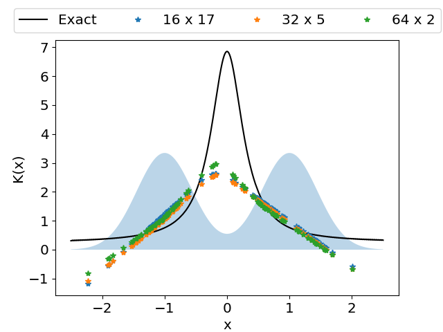
(a) Deep FPF as in Table 1

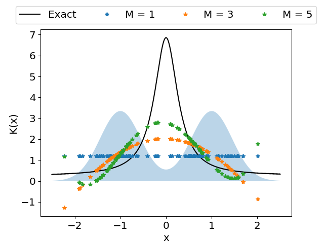
(b) Galerkin with polynomial basis.

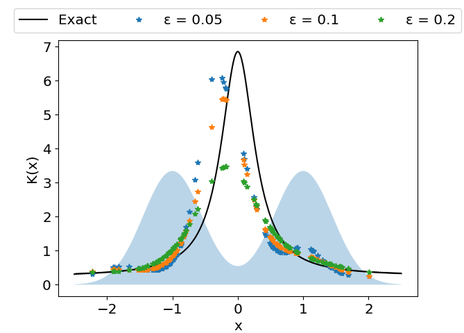
(c) Diffusion Map Based (DM)

Figure 1: Gain function approximation for bimodal example in Section IV-A.

IV-A Illustration with bimodal distribution

The distribution $\rho$ is assumed to be bimodal distribution $\frac{1}{2}N(-1,\sigma^{2})+\frac{1}{2}N(1,\sigma^{2})$ where $\sigma^{2}=0.2$. The proposed numerical procedure in Table 1 is implemented to approximate the gain function. The following three selection of architectures parameters are used

• $2$ layers $64$ neurons each layer

• $5$ layers $32$ neurons each layer

• $17$ layers, $16$ neurons each layer

The three architectures involve same number of unknown weight parameters.

The result is compared with the exact gain. The exact gain function admits a formula in the scalar case given by

$${\sf K}(x)=-\frac{1}{\rho(x)}\int_{-\infty}^{x}\rho(z)(h(z)-\hat{h})dz.$$ (15)

The numerical results are depicted in Figure 1(a): All three architectures produce the same result. For comparison, the Galerkin and diffusion map-based methods are implemented for the bimodal example. The results are depicted in Figure 1(b) and Figure 1(c) respectively. The details of Galerkin algorithm and diffusion map-based algorithm appear in [9] and [14] respectively. The polynomial basis function is used for the Galerkin algorithm.

For this particular example, Deep FPF outperforms Galerkin approximation but does not perform as well as diffusion map based approximation. However, note that there is a lot of room for neural networks to be tuned to produce better result. This is subject of ongoing work.

IV-B Over-fitting with full batch optimization

Consider the application of the proposed procedure on the bimodal example in Section IV-A when the batch-size is equal to the number of samples, i.e. $M=N=100$. The value of the empirical objective function (12) evaluated on the given samples $\{X^{i}\}_{i=1}^{N}$ (training loss), and evaluated on fresh independent samples $\{Y_{i}\}_{i=1}^{N_{1}}$ (test loss), as a function of iteration, are depicted in Figure 2-(a). It is observed that after certain iteration, around $2000$, the test loss starts to increase while the training loss continues to decrease. This illustrates the over-fitting phenomenon. The gap between training loss and test loss is called generalization error.

The over-fitting is avoided when the batch-size is smaller, $M=10$. The training loss and test loss are depicted in 2-(b). It is observed that both training loss and test loss continue to decrease as the iteration number grows. It is also observed that the generalization error remains small. The reason is that random selection of batches at each iteration of the optimization algorithm introduces randomness that prevents over-fitting [20].

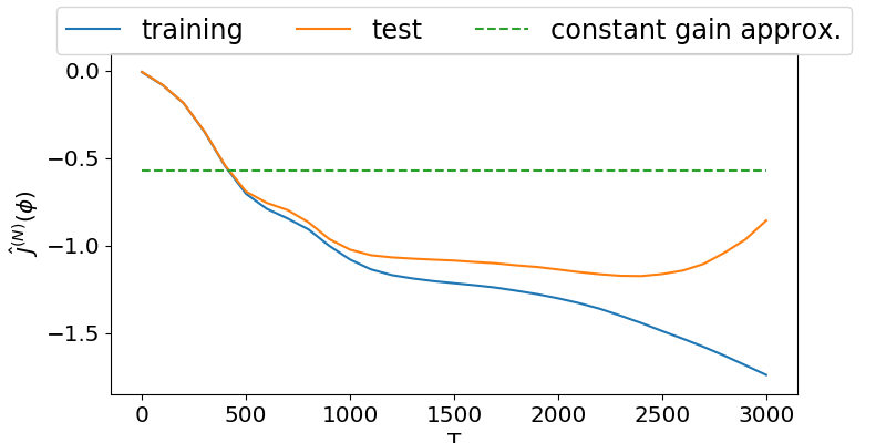
(a) N = M = 100

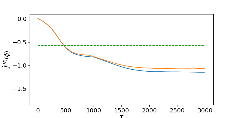
(b) N = 100 and M = 10

Figure 2: The training and test error of the empirical objective function (12) for application the numerical procedure 1 on the bimodal example of Section IV-A.

IV-C Scaling with dimension

Consider the following probability density function

$$\rho(x)=\rho_{b}(x_{1})\prod_{n=2}^{d}\rho_{g}(x_{n}),$$ (16)

for $x=(x_{1},x_{2},...,x_{d})\in\mathbb{R}^{d}$. $\rho_{b}$ is the probability density function for bimodal distribution introduced in Section IV-A and $\rho_{g}$ is the probability density function for $N(0,\sigma^{2})$. Assume that the observation function is $h(x)=x_{1}$. Hence the exact gain function is given by

$$\tilde{\sf K}_{\text{exact}}(x)=({\sf K}_{\text{exact}}(x_{1}),0,...,0),$$ (17)

where ${\sf K}_{exact}(x_{1})$ is given by (15).

Define the m.s.e error according to

$$\text{m.s.e}=\frac{1}{N}\sum_{i=1}^{N}|{\sf K}_{\text{alg.}}(Y^{i})-{\sf K}_{\text{exact}}(Y^{i})|^{2},$$ (18)

where $\{Y^{i}\}_{i=1}^{N}$ are independent samples from $\rho$, and ${\sf K}(\cdot)$ is the approximate gain obtained from the proposed algorithm 1. The m.s.e is computed by averaging over $100$ simulations. The sample size $N=1000$.

The resulting m.s.e as a function of iteration for different dimensions is depicted in Figure 3-(a). It is observed that the dimension does not effect the resulting error to a great degree. For comparison, the m.s.e as a function of dimension, for the proposed approach and the diffusion-map algorithm, is depicted in Figure 3-(b). It is observed that although the m.s.e for diffusion-map is smaller, but it grows faster with dimension compared to the neural- network-based approach. Also, in our simulations we used the optimal value of the kernel-bandwidth for the diffusion-map algorithm for each dimension. In particular $\epsilon=0.1,0.1,0.2,1.0$ for $d=1,2,5,10$ respectively. This hyper parameter tuning may not be possible in application.

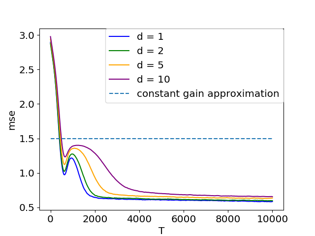
(a) m.s.e as a function of iterations for varying dimensions.

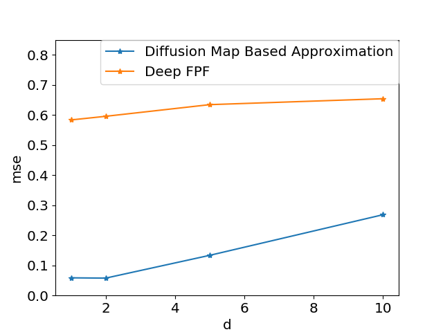
(b) comparison of m.s.e as a function of dimension

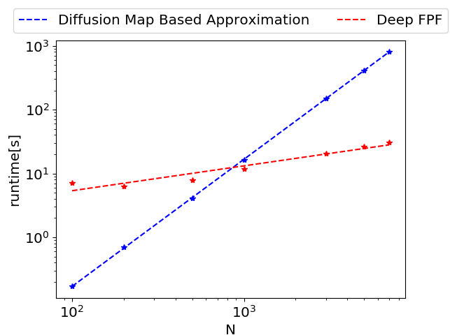
(c) Runtime comparison for Deep FPF and diffusion map based approximation

Figure 3: Numerical analysis of the m.s.e (18) and the runtime for the proposed procedure and comparison with Diffusion-map (DM) and Galerkin approach, for the example in Section IV-C.

IV-D Scaling of computational time with $N$

Comparison of the running-time for the proposed procedure 1 and Diffusion map-based approach as a function of sample size (number of particles) is depicted in Figure 3(c).

It is observed that the running time of the diffusion map based approximation grows with $O(N^{2})$, while the running time of neural network-based approach scales with $O(N)$. This makes the proposed approach favourable for large sample size, which is necessary for high-dimensional problems.

V Application to filtering

Consider the problem of transporting particles from initial distribution (or prior distribution) $\rho_{0}(x)$ to the final distribution (or posterior distribution)

$$\rho_{1}(x)=\frac{\rho_{0}(x)e^{-l(x)}}{\int\rho_{0}(y)e^{-l(y)}\,\mathrm{d}y}.$$

This problem appears in filtering problem with discrete-time observations, where the function $l(x)$ represents the log-likelihood function of the observation model [11, 12, 10].

The transportation is achieved by updating the particles according to

$$\frac{\,\mathrm{d}X^{i}_{t}}{\,\mathrm{d}t}=-\nabla\phi(t,X^{i}_{t}),\quad X^{i}_{0}\sim\rho_{0},\quad t\in[0,1],$$ (19)

where $\phi(t,\cdot)$ is the solution to the Poisson equation (3) with $\rho$ as the distribution of the particles $\{X^{i}_{t}\}_{i=1}^{N}$.

The justification for (19) is as follows. Let $\rho(t,x)$ denote the distribution of the particles $X^{i}_{t}$. We show that $\rho(1,x)$ is equal to the posterior distribution $\rho_{1}(x)$. The evolution of $\rho(t,x)$ is given by the continuity equation

$$\frac{\partial\rho}{\partial t}(t,x)=\nabla\cdot(\rho(t,x)\nabla\phi(t,x)),\quad\rho(0,x)=\rho_{0}(x),$$

which is equal to

$$\frac{\partial\rho}{\partial t}(t,x)=-\rho(t,x)(h(x)-\hat{h}_{t}),\quad\rho(0,x)=\rho_{0}(x),$$

because $\phi(t,x)$ solves the Poisson equation (3). The solution to this pde is

$$\rho(t,x)=\frac{\rho_{0}(x)e^{-th(x)}}{\int\rho_{0}(y)e^{-th(y)}\,\mathrm{d}y},$$ (20)

concluding $\rho(1,x)=\rho_{1}(x)$. The trajectory $\rho(t,x)$ is known as the homotopy between $\rho_{0}$ and $\rho_{1}$.

For example, let $\rho_{0}$ be a Gaussian distribution $N(0,1)$ and let $l(x)=(|x|-2)^{2}$. This likelihood model induces a bimodal posterior distribution. The resulting flow of particles, with $\nabla\phi(t,x)$ computed according to the proposed algorithm 1, the diffusion map-based algorithm with $\epsilon=0.1$, and the Galerkin algorithm with fifth order polynomial basis functions, is depicted in Figure 4(a). The figure shows a kernel-density estimate of the empirical distribution of the particles along with the exact distribution $\rho(t,x)$ at three time instants: $t=0,0.5,1.0$.

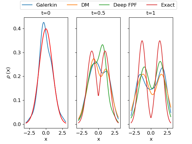
(a)

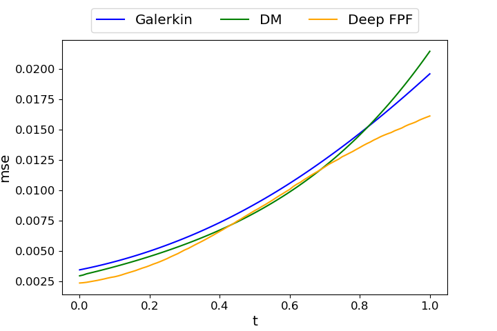
(b)

Figure 4: The empirical distribution of the particles simulated according to (19) where $\nabla\phi$ is approximated using three different algorithms: Neural network-based, Diffusion map-based (DM), and Galerkin. (a) shows a kernel density estimate of the empirical distribution along with the exact distribution given by the homotopy (20). (b) shows m.s.e in estimating the conditional expectation of $\psi(x)={1}_{x>0}$ computed according to (21) for the filtering example of Section V.

A quantitative comparison is provided by calculating the mean square error in estimating the conditional expectation of the function $\psi(x)=x{1}_{x>0}$ over time. The m.s.e is defined according to

$${mse}_{t}=\frac{1}{K}\sum_{k=1}^{K}(\frac{1}{N}\sum_{i=1}^{N}\psi(X_{t}^{k,i})-\int\psi(x)\rho(t,x)dx)^{2},$$ (21)

where $K=100$ is the number of independent simulations. The result is depicted in Figure 4(b).

Remark 1

In a filtering application, it is not necessary to reinitialize the neural network for gain function approximation after each time the particles are moved. Because the particles move slightly at each time step, the gain function does not vary much. Therefore, the gain function that is obtained in the previous filtering step is a good initialization. This reduces the required number of iterations for gain function approximation significantly.

VI Conclusion

We presented a deep learning-based approach to approximate the gain function in feedback particle filter, and provided preliminary numerical results that serves as proof of concept. There are two main directions of future work: (i) sample complexity analysis of the proposed procedure in terms of neural network architecture. This requires non-trivial application of the existing generalization theory results, because the objective function involves gradient of the neural net evaluated on samples which is not standard; (ii) numerical analysis of the proposed procedure for high-dimensional filtering problems and comparison with importance sampling-based particle filters.

References

- [1] J. Xiong, An introduction to stochastic filtering theory, ser. Oxford Graduate Texts in Mathematics. Oxford University Press, 2008, vol. 18.
- [2] N. J. Gordon, D. J. Salmond, and A. F. Smith, “Novel approach to nonlinear/non-Gaussian Bayesian state estimation,” in IEE Proceedings F (Radar and Signal Processing), vol. 140, 1993, pp. 107–113.
- [3] A. M. Doucet, A.and Johansen, “A tutorial on particle filtering and smoothing: Fifteen years later,” Handbook of Nonlinear Filtering, vol. 12, pp. 656–704, 2009.
- [4] P. Bickel, B. Li, T. Bengtsson et al., “Sharp failure rates for the bootstrap particle filter in high dimensions,” in Pushing the limits of contemporary statistics: Contributions in honor of Jayanta K. Ghosh. Institute of Mathematical Statistics, 2008, pp. 318–329.
- [5] T. Bengtsson, P. Bickel, and B. Li, “Curse of dimensionality revisited: Collapse of the particle filter in very large scale systems,” in IMS Lecture Notes - Monograph Series in Probability and Statistics: Essays in Honor of David F. Freedman. Institute of Mathematical Sciences, 2008, vol. 2, pp. 316–334.
- [6] C. Snyder, T. Bengtsson, P. Bickel, and J. Anderson, “Obstacles to high-dimensional particle filtering,” Monthly Weather Review, vol. 136, no. 12, pp. 4629–4640, 2008.
- [7] P. Rebeschini, R. Van Handel et al., “Can local particle filters beat the curse of dimensionality?” The Annals of Applied Probability, vol. 25, no. 5, pp. 2809–2866, 2015.
- [8] T. Yang, P. G. Mehta, and S. P. Meyn, “Feedback particle filter,” IEEE Transactions on Automatic Control, vol. 58, no. 10, pp. 2465–2480, October 2013.
- [9] T. Yang, R. S. Laugesen, P. G. Mehta, and S. P. Meyn, “Multivariable feedback particle filter,” Automatica, vol. 71, pp. 10–23, 2016.
- [10] T. Yang, H. A. Blom, and P. G. Mehta, “The continuous-discrete time feedback particle filter,” in 2014 American Control Conference. IEEE, 2014, pp. 648–653.
- [11] F. Daum, J. Huang, and A. Noushin, “Exact particle flow for nonlinear filters,” in SPIE Defense, Security, and Sensing, 2010, pp. 769 704–769 704.
- [12] ——, “Generalized Gromov method for stochastic particle flow filters,” in SPIE Defense+ Security. International Society for Optics and Photonics, 2017, pp. 102 000I–102 000I.
- [13] A. Taghvaei and P. G. Mehta, “Gain function approximation in the feedback particle filter,” in Decision and Control (CDC), 2016 IEEE 55th Conference on. IEEE, 2016, pp. 5446–5452.
- [14] A. Taghvaei, P. G. Mehta, and S. P. Meyn, “Diffusion map-based algorithm for gain function approximation in the feedback particle filter,” arXiv preprint arXiv:1902.07263v2, 2019. [Online]. Available: https://arxiv.org/abs/1902.07263
- [15] L. Lu, X. Meng, Z. Mao, and G. E. Karniadakis, “DeepXDE: A deep learning library for solving differential equations,” arXiv preprint arXiv:1907.04502, 2019. [Online]. Available: https://arxiv.org/abs/1907.04502
- [16] J. Sirigano and K. Spiliopoulos, “DGM: A deep learning algorithm for solving partial differential equations,” Journal of Computational Physics, vol. 375, pp. 1339–1364, 2018.
- [17] E. Weinan and Y. Bing, “The deep Ritz method: A deep learning-based numerical algorithm for solving variational problems,” Communications in Mathematics and Statistics, vol. 6, no. 1, pp. 1–12, 2018.
- [18] R. S. Laugesen, Linear Analysis and Partial Differential Equations. Lecture notes, 2015.
- [19] D. P. Kingma and J. Ba, “Adam: A method for stochastic optimization,” in 3rd International Conference for Learning Representations, 2017.
- [20] L. Bottou, “Large-scale machine learning with stochastic gradient descent,” in Proceedings of COMPSTAT’2010. Springer, 2010, pp. 177–186.