IQ Collaboratory II: The Quiescent Fraction of Isolated, Low Mass Galaxies Across Simulations and Observations

Abstract

We compare three major large-scale hydrodynamical galaxy simulations (EAGLE, Illustris-TNG, and SIMBA) by forward modeling simulated galaxies into observational space and computing the fraction of isolated and quiescent low mass galaxies as a function of stellar mass. Using SDSS as our observational template, we create mock surveys and synthetic spectroscopic and photometric observations of each simulation, adding realistic noise and observational limits. All three simulations show a decrease in the number of quiescent, isolated galaxies in the mass range $\mathrm{M_{*}}=10^{9-10}\ \mathrm{M_{\odot}}$, in broad agreement with observations. However, even after accounting for observational and selection biases, none of the simulations reproduce the observed absence of quiescent field galaxies below $\mathrm{M_{*}}=10^{9}\ \mathrm{M_{\odot}}$. We find that the low mass quiescent populations selected via synthetic observations have consistent quenching timescales, despite apparent variation in the late time star formation histories. The effect of increased numerical resolution is not uniform across simulations and cannot fully mitigate the differences between the simulations and the observations. The framework presented here demonstrates a path towards more robust and accurate comparisons between theoretical simulations and galaxy survey observations, while the quenching threshold serves as a sensitive probe of feedback implementations.

1 Introduction

The transition of galaxies from star-forming into quiescence provides key insights into the physical processes that drive galaxy evolution. Major extragalactic surveys like the Sloan Digital Sky Survey (SDSS, York et al., 2000) have been instrumental in quantifying the differing properties of galaxies in these two categories, including morphology, environment, and color (e.g., Blanton et al., 2003; Kauffmann et al., 2003; Brinchmann et al., 2004; Blanton & Moustakas, 2009; Moustakas et al., 2013). The processes that drive a galaxy’s transformation can be broadly divided into two categories: external processes which occur in high-density environments and processes internal to the galaxy which are often thought to be correlated to galaxy mass (e.g., Peng et al., 2010).

Understanding how and when feedback mechanisms operate within galaxies and in which regimes they are most effective remains a major focus of both observational and theoretical studies of galaxy evolution. Observational galaxy surveys have been used to characterize the populations of quiescent and star forming galaxies as a function of stellar mass (Kauffmann et al., 2004; Geha et al., 2012), environment (Wetzel et al., 2012), and redshift (Brammer et al., 2009); as well as key correlations between galaxy properties (e.g., the star forming sequence; Daddi et al., 2007; Noeske et al., 2007; Salim et al., 2007; Elbaz et al., 2007) which inform our understanding of the underlying forces that drive galaxy evolution.

Large-scale cosmological hydrodynamic galaxy formation simulations reproduce the observed universe in a qualitative manner (Genel et al., 2014; Vogelsberger et al., 2014; Schaye et al., 2015; Davé et al., 2017; Pillepich et al., 2018a; Davé et al., 2019). Each simulation uses a distinct set of approximations for the complex physics of underlying galaxy evolution, including star formation, heating and cooling of gas, black hole formation and growth, feedback from active galactic nuclei (AGN), and stellar feedback (for an overview see Somerville & Davé, 2015; Vogelsberger et al., 2020). While it has been shown that many different subgrid models can produce relatively consistent pictures of galaxy evolution (Naab & Ostriker, 2017), the variations between simulations present a unique opportunity to explore how feedback mechanisms shape galaxy evolution.

Many studies have focused on comparing the simulated distributions of quantities such as galaxy masses, colors, or star-formation rates to observations (e.g., Genel et al., 2014; Torrey et al., 2014; Vogelsberger et al., 2014; Schaye et al., 2015; Somerville & Davé, 2015; Sparre et al., 2015; Davé et al., 2017; Pillepich et al., 2018a; Nelson et al., 2018; Trayford et al., 2017; Donnari et al., 2019, 2020a, 2020b). These works primarily focus on comparing a singular simulation to a particular set of observations. Studies using multiple simulations require the careful construction of a consistent framework for inter-simulation comparison.

In the observed universe, the quiescent fraction for isolated galaxies is zero at $\mathrm{M_{*}}<10^{9}\ \mathrm{M_{\odot}}$ (Geha et al., 2012) in the SDSS volume, suggesting that feedback in this mass regime is highly sensitive to stellar mass. Most studies of feedback in low mass galaxies have focused on environmental quenching, either in the context of high density environments such as clusters or interactions with a Milky Way-like host galaxy (e.g., Fillingham et al., 2018; Sales et al., 2015; Wetzel et al., 2013, 2015).

Internal feedback may influence galaxy evolution down to $\mathrm{M_{*}}\sim 10^{9}\ \mathrm{M_{\odot}}$, via either AGN (Dickey et al., 2019; Koudmani et al., 2019; Penny et al., 2018) or stellar feedback (El-Badry et al., 2016). However, the efficiency and interplay of different feedback mechanisms below this mass limit remains uncertain. Large-scale hydrodynamic simulations present a unique opportunity to create an “observed” magnitude limited galaxy survey and explore how different subgrid feedback implementations shape the distribution.

The IQ (Isolated & Quiescent) Collaboratory aims to bridge the gap between simulations and observations of star-forming and quiescent galaxies to better characterize internal quenching processes. In Hahn et al. (2019, Paper I), we began the process of comparing the star forming sequence across a set of simulations.

Our initial analysis in Paper I highlighted the large variation in the apparent quiescent populations of each simulation, but we did not make a direct comparison between simulations and observations. In that work, the star formation rates from the simulations are obtained “directly” from the simulation output, as opposed to being derived from “observables” like H$\mathrm{\alpha}$- or UV+IR-derived star formation rates, or indices such as the H$\mathrm{\alpha}$ equivalent width (EW) and $\mathrm{D_{n}4000}$, an index that measures the strength of the $4000\mbox{\AA}$ break and loosely traces stellar age. Moreover, even within observational results, selecting different tracers for e.g., SFRs can give rise to significant variation (e.g., Salim et al., 2007; Kennicutt & Evans, 2012; Speagle et al., 2014; Flores Velázquez et al., 2020; Katsianis et al., 2020)

In addition to deriving galaxy observables from a simulation, fully transforming a simulated volume into a true observational analogue requires the careful creation of complete, volume-corrected samples. This is particularly challenging when we are trying to reproduce observations comparing star forming and quiescent populations, which often suffer from differing levels of incompleteness within the same survey.

Our goal in this work is to create an “apples-to-apples” comparison of the quiescent fraction of isolated low mass ($\mathrm{M_{*}}<10^{10}\ \mathrm{M_{\odot}}$) galaxies as a function of stellar mass, using observations of the local universe and a set of simulations, all of which produce realistic cosmological volumes using distinct implementations of subgrid physics. We focus our study on a selection of three major cosmological hydrodynamic simulations (EAGLE, Illustris-TNG, and SIMBA) and compare them to the observed population of low mass quiescent galaxies in the Sloan Digital Sky Survey (SDSS).

In Section 2, we present the simulations used in this work and in Section 3 we discuss the observations which serve as our point of comparison. In Section 4, we create mock observations from each simulation, including synthetic spectra, realistic noise, and SDSS-like incompleteness. Section 5 compares the “observed” simulations to the distribution of low mass quiescent galaxies in SDSS. In Section 7 we explore the star formation histories of quiescent galaxies in the simulations and we review our findings in Section 8.

2 Galaxy Formation Simulations

In this work, we focus on three large-scale hydrodynamic cosmological simulations (EAGLE, Illustris-TNG, and SIMBA), which we will compare to observations. We provide brief descriptions of each simulation below.

2.1 EAGLE

The Virgo Consortium’s Evolution and Assembly of GaLaxies and their Environment (EAGLE) project (Schaye et al., 2015; Crain et al., 2015; McAlpine et al., 2016) has a volume of (100 Mpc)³ (co-moving), with dark matter and baryonic particle masses of $9.6\times 10^{6}\ \mathrm{M_{\odot}}$ and $1.8\times 10^{6}\ \mathrm{M_{\odot}}$. The simulation uses ANARCHY (Dalla Vecchia, in prep.), a modified version of the Gadget3 N-body SPH code (Springel et al., 2001b; Springel, 2005; Schaller et al., 2015). The subgrid model for feedback from massive stars and AGN is based on thermal energy injection in the interstellar medium (Dalla Vecchia & Schaye, 2012). The subgrid parameters were calibrated to reproduce the $z=0$ stellar mass function and galaxy sizes.

Previous works that have reproduced observables and examined the quenched population of the EAGLE simulation include Schaye et al. (2015), Furlong et al. (2015), Trayford et al. (2015) and Trayford et al. (2017), and the galaxy–black hole relations are discussed in McAlpine et al. (2017, 2018); Bower et al. (2017); Habouzit et al. (2020). Trčka et al. (2020) show that mock spectral energy distributions (see Camps et al., 2018 for public release of the SEDs) based on EAGLE galaxies and radiative transfer calculations using skirt (Baes et al., 2011) are in overall agreement with observed galaxy spectra, and highlight the need for consistent comparisons between simulations and observations. Trayford et al. (2017) used the same results of the skirt radiative transfer code to determine quenched fractions based on mock UVJ colors, along with the distribution of H$\mathrm{\alpha}$ flux and $\mathrm{D_{n}4000}$. They found that the passive fraction varies significantly depending on the definition of quenched. We will compare our results to previous conclusions in § 6.1.1.

2.2 Illustris-TNG

The Next Generation Illustris project (IllustrisTNG or TNG) (Marinacci et al., 2018; Naiman et al., 2018; Nelson et al., 2018; Pillepich et al., 2018a; Springel et al., 2018) is the successor to the original Illustris project (Genel et al., 2014; Vogelsberger et al., 2014), with significant updates in the subgrid models and physics included in the simulation. We use the TNG100 simulation, which has a volume of (110.7 Mpc)³, and dark matter and baryonic mass resolutions of $7.6\times 10^{6}\ \mathrm{M_{\odot}}$ and $1.4\times 10^{6}\ \mathrm{M_{\odot}}$. TNG is run using the AREPO moving-mesh code (Springel, 2010), which is based on the Gadget code (Springel et al., 2001b; Springel, 2005). Adjustments in the TNG model include the addition of magneto-hydrodynamics, updated stellar feedback prescriptions, and the transition from thermal “bubbles” in the IGM to a BH-driven kinetic wind for the low-accretion-rate black hole feedback mode (Pillepich et al., 2018b; Weinberger et al., 2017).

The color bimodality of low-redshift galaxies is shown to compare well to SDSS (Nelson et al., 2018). Other papers describe the size evolution of quiescent galaxies (Genel et al., 2018), and correlations between galaxy properties and super massive black holes and AGN feedback (Weinberger et al., 2018; Habouzit et al., 2019; Terrazas et al., 2020; Davies et al., 2020; Li et al., 2019; Habouzit et al., 2020). Donnari et al. (2019) show quenched fractions based on UVJ selection and the star forming sequence, and compare these to UVJ-selected observed quenched fractions from COSMOS/UltraVISTA (Muzzin et al., 2013). Donnari et al. (2020a) and Donnari et al. (2020b) explore the quenched fraction derived using star formation rates and distances from the galaxy star-forming sequence. Donnari et al. (2020a) in particular explores how systematic uncertainties effect a single set of observations, which we will further discuss in § 6.1.2.

2.3 SIMBA

SIMBA (Davé et al., 2019) is a suite of cosmological simulations built on the GIZMO meshless finite mass hydrodynamics code (Hopkins, 2015, 2017), also based on the Gadget code (Springel et al., 2001b; Springel, 2005), and forms the next generation of the MUFASA (Davé et al., 2016) simulations with novel black hole growth and feedback sub-grid models. The fiducial run has a volume of $(143\ \mathrm{Mpc})^{3}$ and dark matter and baryonic mass resolutions of $9.6\times 10^{7}\ \mathrm{M_{\odot}}$ and $1.8\times 10^{7}\ \mathrm{M_{\odot}}$, respectively.

SIMBA includes a model for on-the-fly dust production and destruction (broadly following McKinnon et al., 2017), and star formation is regulated with two-phase kinetic outflows, which were tuned to predictions from the Feedback in Realistic Environments (FIRE) simulations (Hopkins et al., 2014; Muratov et al., 2015; Anglés-Alcázar et al., 2017b; Hopkins et al., 2018). Black hole growth in SIMBA is based on the torque-limited accretion model (Hopkins & Quataert, 2011; Anglés-Alcázar et al., 2013, 2015; Anglés-Alcázar et al., 2017a) linking the black hole accretion to properties of the galaxy’s inner gas disk. The AGN feedback consists of kinetic bipolar outflows, modeled after observed outflows of AGN, and X-ray feedback input in the surrounding gas similar to Choi et al. (2012).

Previous work using SIMBA has already discussed the radial density profiles of quenched galaxies (Appleby et al., 2019), the weak correlation between galaxy mergers and quenching (Rodríguez Montero et al., 2019), and the connection between quenching and black hole growth (Davé et al., 2019; Thomas et al., 2019; Habouzit et al., 2020). We compare our results to relevant studies in § 6.1.3.

3 Observations

Following Geha et al. (2012), we build our sample of observed galaxies from SDSS, using the NASA/Sloan Atlas (NSA; Blanton et al., 2011), which includes all galaxies within $z<0.055$ in the SDSS footprint. The NASA/Sloan Atlas is a re-reduction of SDSS DR8 (Aihara et al., 2011) optimized for nearby low-luminosity objects (Yan, 2011; Yan & Blanton, 2012), including an improved background subtraction technique (Blanton et al., 2011) and the addition of near and far UV photometry from GALEX. The catalog includes emission line fluxes and equivalent widths for all galaxies. We calculate stellar masses as in Mao et al. (2020), using the Bell et al. (2003) relation to determine mass-to-light ratio from the $g-r$ color. See Section 5.3 for a more in-depth discussion on the effects of uncertainty in the stellar mass measurements on the resultant quiescent fraction.

As in Geha et al. (2012), we consider a low mass galaxy to be quiescent if it has little-to-no star formation and is dominated by older stellar populations. For the first condition, we use the H$\mathrm{\alpha}$ equivalent width (EW), which traces recent ($<10$ Myr) star formation, and require H$\mathrm{\alpha}$ EW $<2$ Å. To probe galaxy age, we rely on $\mathrm{D_{n}4000}$ (Balogh et al., 1999), an index which quantifies the strength of the $4000\,$Å break in the spectrum and traces the light-weighted age of the stellar population. The $\mathrm{D_{n}4000}$ index is an indirect measure of intermediate (${\sim}1$ Gyr) star formation (Hamilton, 1985; Moustakas et al., 2006; Brinchmann et al., 2004). We use the empirical relation of Geha et al. (2012): $\mathrm{D_{n}4000}$ $>0.6+0.1\log_{10}(\mathrm{M_{*}}/\mathrm{M_{\odot}})$, to select galaxies with older stellar populations.

To quantify the environment of each low mass galaxy, we use $\mathrm{d}_{\mathrm{{host}}}$, which is defined as the projected distance to the nearest massive neighbor ($\mathrm{M_{*}}>2.5\times 10^{10}\ \mathrm{M_{\odot}}$; $\mathrm{M_{K_{s}}}<-23$; hereafter the host galaxy). We search for potential host galaxies within 7 Mpc and 1000 km/s of each low mass galaxy, using the Two Micron All Sky Survey (2MASS) Extended Source Catalog to ensure we do not miss any potential host galaxies that lie outside the SDSS imaging footprint. In the few cases where we do not identify a host within 7 Mpc, we use $\mathrm{d}_{\mathrm{{host}}}$= 7 Mpc.

We define galaxies as isolated when $\mathrm{d}_{\mathrm{{host}}}$ $>1.5$ Mpc. This is an empirical choice based on the behavior of the quiescent fraction as a function of $\mathrm{d}_{\mathrm{{host}}}$ (see Fig. 4 of Geha et al. (2012) or Figure 5 in this work). The quiescent fraction only shows a dependence on environment for $\mathrm{d}_{\mathrm{{host}}}$ $<1.5$ Mpc, and so we consider low mass galaxies beyond this threshold to be isolated. Using a less strict definition (e.g., galaxies are isolated beyond $\mathrm{d}_{\mathrm{{host}}}$ $=1$ Mpc) shifts the quenching threshold to a slightly lower mass, while a more conservative definition does not change the observed threshold. For galaxies with stellar masses above $\mathrm{M_{*}}=10^{10}\ \mathrm{M_{\odot}}$, we use the central – satellite designation from the group catalog of Tinker et al. (2011).

In the left column of Figure 1, we show the distribution of isolated galaxies observed in the local universe as a function of $\mathrm{D_{n}4000}$ and SDSS $r$ magnitude in the mass range $\mathrm{M_{*}}=10^{8-10}\ \mathrm{M_{\odot}}$. Galaxies in isolation are only observed to be quiescent above $\mathrm{M_{*}}=10^{9}\ \mathrm{M_{\odot}}$, (Figure 2).

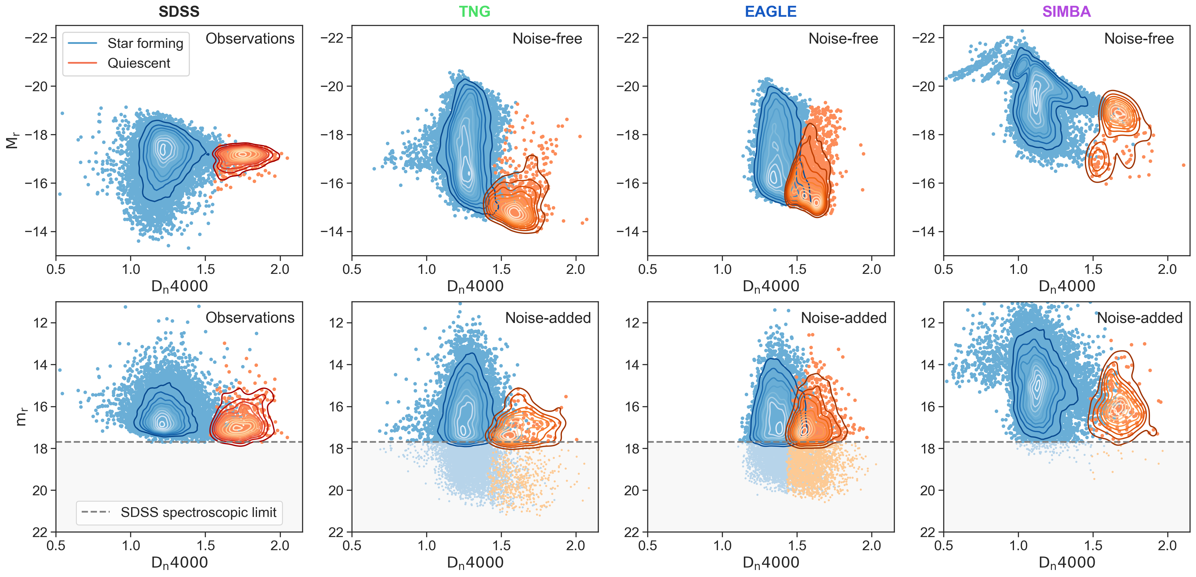
Figure 1: Top row: The distribution of absolute $r$ magnitude ($\mathrm{M_{r}}$) as a function of $\mathrm{D_{n}4000}$, from SDSS for observations and derived from the noise-less synthetic spectra from each simulation (from left to right: TNG, EAGLE, and SIMBA), for isolated galaxies (based on $\mathrm{d}_{\mathrm{{host}}}$) in the stellar mass range $\mathrm{M_{*}}=10^{8-10}\ \mathrm{M_{\odot}}$. Galaxies are color-coded as star forming (blue) or quiescent (orange) based on the noise-free H$\mathrm{\alpha}$ EW and $\mathrm{D_{n}4000}$. Bottom row: The distribution of apparent $r$ magnitude ($\mathrm{m_{r}}$) as a function of $\mathrm{D_{n}4000}$, derived from the noise-added synthetic spectra along a single random sightline through each simulation box. Galaxies are color-coded as star forming (blue) or quiescent (orange) based on the noise-added H$\mathrm{\alpha}$ EW and $\mathrm{D_{n}4000}$. Galaxies below the gray dashed line fall below the SDSS spectroscopic limit and would not be selected for spectroscopic follow-up in SDSS. As such, they are not included in the calculation of $f_{q}$ along a given sightline.

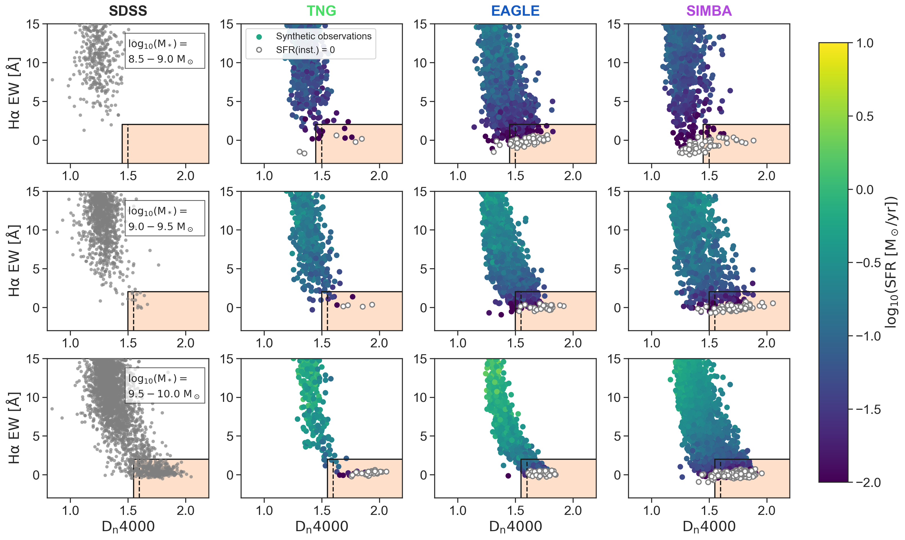
Figure 2: $\mathrm{D_{n}4000}$ vs. H$\mathrm{\alpha}$ EW, from SDSS for observations and derived from the noise-added synthetic spectra from each simulation (from left to right: TNG, EAGLE, and SIMBA), for isolated galaxies (based on $\mathrm{d}_{\mathrm{{host}}}$) in three stellar mass bins (from top to bottom: $\mathrm{M_{*}}=10^{8.5-9.0}\ \mathrm{M_{\odot}}$, $10^{9.0-9.5}\ \mathrm{M_{\odot}}$, and $10^{9.5-10.0}\ \mathrm{M_{\odot}}$). Galaxies are observed as quiescent if they fall into the orange region of $\mathrm{D_{n}4000}$-H$\mathrm{\alpha}$ EW parameter space. The $\mathrm{D_{n}4000}$ limit depends on stellar mass and is equal to the solid (dashed) vertical line at the low mass (high-mass) end of the bin for each row. For the simulations, galaxies are color-coded by their instantaneous star formation rates, and galaxies with SFR $=0\ \mathrm{M_{\odot}/yr}$ are shown in white.

4 Mock Observations

To create a true apples-to-apples comparison between the observations and simulations, we must account for the effects of observational incompleteness, finite signal to noise, and a lack of precise distance information for individual galaxies in a wide-field survey.

To that end, we create mock surveys and synthetic observations of each simulation, adding realistic noise and observational limits. We use SDSS as our observational template. We select the mock observational limits and injected noise to match SDSS. We apply the same methodology to all the simulations, as described below for a single simulation box. However, this method can also be generalized and applied to semi-analytic models and zoom-in simulations, as well as adapted to match other surveys and observations.

4.1 Synthetic spectra

We begin by generating synthetic spectra for all galaxies in a given simulation using FSPS (Flexible Stellar Population Synthesis; Conroy et al., 2009; Conroy & Gunn, 2010, and the Python interface python-fsps Foreman-Mackey et al., 2014). Our method is described in full in Starkenburg et. al (in prep.), but in brief it is as follows.

For each galaxy, we bin the total stellar mass formed by formation age ($t$) and stellar metallicity ($Z$). We use a uniform $t,Z$ grid across all the simulations to standardize the effects of otherwise variable time resolution and particle size. Age bin size increases linearly as a function of lookback time based on the minimum age steps of the underlying SSP models, from $t$ = 0 to $t$ = 13.75 Gyr. The metallicity grid spans $\mathrm{\log_{10}(Z/\mathrm{Z_{\odot}})}=-2.2$ to $0.5$ with $\Delta Z=0.3$ at low metallicity, with bin resolution increasing to $\Delta Z=0.1$ near $Z=0$. We use a Chabrier (2003) IMF throughout, and include the AGB dust emission model of Villaume et al. (2015). To cover the most recent star formation and avoid resolution effects of stellar particles, we set the star formation rates younger than 15 Myr equal to the instantaneous star formation rate from the galaxy’s gas particles with metallicity equal to the current mass-weighted metallicity of the star-forming gas.

We generate the spectrum of a simple stellar population at each point in the $t,Z$ grid. The sum of the SPS spectra, weighted by the stellar mass formed, produces the galaxy spectrum. The nebular emission lines are calculated independently for each stellar metallicity bin using the FSPS nebular emission line prescription based on a CLOUDY lookup table (Byler et al., 2017), with the gas metallicity fixed to that of the metallicity bin.

Dust forms a crucial component to consider when building mock observables and when analyzing observational data, and different dust models can strongly affect results and conclusions. However, for lower-mass galaxies with relatively low gas masses and low metallicities, dust is expected to affect results less strongly. We therefore apply the well-known and often used two-component dust model from Charlot & Fall (2000), which consists of a dust screen with a power law dust attenuation curve with index $\Gamma=-0.7$ and a normalization of $\tau(5500\mbox{\AA})=0.33$. Stars younger than 30 Myr are additionally attenuated following an identical power-law attenuation curve with $\tau(5500\mbox{\AA})=1.0$. We discuss the effects of using different dust models in building mock spectra in Starkenburg et al. (in prep.).

Hahn et al. (in prep.) use approximate Bayesian computation to infer an empirical dust model using the same set of mock galaxy spectra by fitting SDSS $r$-band magnitudes, $g-r$ colors, and NUV-FUV colors. We have tested how results in the present work change when using the best-fit dust empirical model. While the H$\mathrm{\alpha}$ EW measurements can be significantly affected by changing the dust model, $\mathrm{D_{n}4000}$ is relatively unchanged, as the index is not strongly sensitive to dust attenuation.

Using the synthetic spectra, we generate SDSS g and r band magnitudes, as well as $\mathrm{D_{n}4000}$ and H$\mathrm{\alpha}$ EW for all galaxies (Figure 1, top row). These quantities are noise-free and derived from spectra which encompass the total stellar light of each galaxy.

4.2 Mock surveys

In generating synthetic photometric and spectroscopic quantities for each simulated galaxy, we are much closer to observational analogues for each simulation. However, the distribution of absolute magnitude and $\mathrm{D_{n}4000}$ shown in the top row of Figure 1 for each simulation are not directly comparable to the corresponding distribution in SDSS (upper left), as the simulations are unaffected by observational noise and each sample contains every galaxy in the simulation volume. To accurately match observations, we need to create mock surveys of each simulation box.

Our method for creating mock surveys is as follows:

1. Place an “observer” at a random location 10 Mpc outside the simulation volume. This distance is selected to match the lower distance limit on galaxies in the NSA catalog from SDSS.

2. Calculate apparent magnitudes, radial velocities, and projected distances for all galaxies as the observer would see them “on sky”. For each galaxy, the radial velocity is the sum of the peculiar velocities along the observer’s sightline and the recessional velocities given the distance between the galaxy and observer.

3. Convolve the synthetic spectra with the SDSS instrumental line spread profile (modeled as a Gaussian with $\sigma=70$ km/s) and resample the spectra to match the SDSS wavelength resolution and coverage.

4. Add realistic spectral noise. The average signal to noise ratio (SNR) of SDSS spectra is dependent on galaxy color and apparent magnitude, and is also a function of wavelength. To reproduce the noise characteristics of SDSS, we bin galaxies from SDSS as a function of $g-r$ color and apparent r magnitude. In each bin, we randomly draw 50 spectra and calculate the average SNR at each wavelength. In each mock observer’s frame, noise is added to the synthetic spectra based on galaxy color, apparent magnitude and wavelength by drawing from a normal distribution $\sigma(\lambda,\ g-r,\ m_{r})$ such that the SNR matches the SDSS model. For simulated galaxies which fall outside the populated regions of the SDSS color-magnitude diagram, we select the closest bin in color-magnitude space.

5. Calculate stellar masses from the $g-r$ colors, following the prescription of Mao et al. (2020). Notably, this can result in stellar mass estimates that appear lower than the resolution limits of the simulation.

6. Remeasure $\mathrm{D_{n}4000}$ and H$\mathrm{\alpha}$ EW from the noise-added and instrumentally-broadened spectra. Figure 2 shows the distribution of noise-added $\mathrm{D_{n}4000}$ and H$\mathrm{\alpha}$ EW for the simulations in three stellar mass bins, as compared to SDSS. We follow the definition of Balogh et al. (1999) for $\mathrm{D_{n}4000}$ measurements and Yan et al. (2006) for H$\mathrm{\alpha}$ EW measurements.

7. Remove “unobservable” galaxies from the sample. Spectroscopy was only acquired for galaxies in SDSS above the limiting magnitude $m_{r}=17.7$. To accurately match SDSS, simulated galaxies which have apparent magnitudes fainter than 17.7 along a particular sightline must be removed from the sample.

In Figure 1, we show effects of adding realistic noise, velocity resolution, and completeness cuts to isolated, $\mathrm{M_{*}}<10^{10}\ \mathrm{M_{\odot}}$ galaxies in each of the three simulations. The upper row shows absolute magnitude ($M_{r}$) and $\mathrm{D_{n}4000}$ calculated from the noise-free synthetic spectra, while the bottom row shows $\mathrm{D_{n}4000}$ measured from the noise-added spectra and the apparent magnitudes ($m_{r}$) as seen by the observer along a random sightline.

The gray region in each panel in the bottom row of Figure 1 represents the regime in which galaxies are too faint to be selected for spectroscopic follow up with SDSS. Of the three simulations, SIMBA produces the fewest “unobservable” galaxies. This is likely driven by the fact the SIMBA does not resolve galaxies all the way down to $\mathrm{M_{*}}=10^{8}\ \mathrm{M_{\odot}}$, leading to fewer faint galaxies which are then preferentially removed from the observed sample (see Section 5.2 for a more detailed discussion on the effects of resolution in each simulation). TNG has the faintest population of quiescent galaxies in absolute magnitude (at least in part because it extends to the lowest stellar masses) and correspondingly fewer quiescent galaxies from this simulation are observable with an SDSS-like survey.

In Figure 2, we show the distribution of $\mathrm{D_{n}4000}$ and H$\mathrm{\alpha}$ EW in three stellar mass bins for the observations and for the simulations as measured from the noise-added spectra. We color-code the simulations by instantaneous SFR, highlighting the need for synthetic observations to select the analogous quiescent population from simulations. As shown in Geha et al. (2012), no quiescent galaxies are observed in the SDSS volume below $\mathrm{M_{*}}=10^{9}\ \mathrm{M_{\odot}}$.

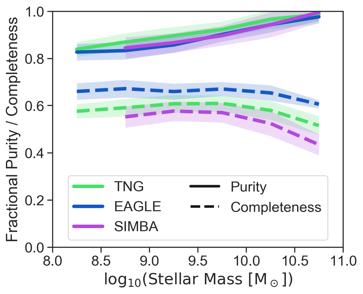
Figure 3: The purity (the fraction of galaxies selected as isolated by the $\mathrm{d}_{\mathrm{{host}}}$ criterion which are centrals, solid lines) and completeness (the fraction of the population of centrals which appear as isolated when using $\mathrm{d}_{\mathrm{{host}}}$, dashed lines) of the $\mathrm{d}_{\mathrm{{host}}}$ isolation criteria compared to the central/satellite classification from the simulations themselves. Shaded regions represent the one-sigma variation across 10 randomly oriented sightlines. Using the $\mathrm{d}_{\mathrm{{host}}}$ criterion selects a sample of galaxies that is relatively pure ($>85$ % of isolated galaxies are centrals) but somewhat incomplete (only $55-70$ % of centrals are selected as isolated). We use the true simulation-based stellar masses in this figure to provide maximum clarity on the purity and completeness of the $\mathrm{d}_{\mathrm{{host}}}$ criterion.

4.3 Isolation criteria

As in the observations, we select galaxies as isolated based on $\mathrm{d}_{\mathrm{{host}}}$, the projected distance between each simulated galaxy and its most nearby massive neighbor. As in the observations, for each galaxy we identify potential hosts (galaxies with ($\mathrm{M_{*}}>2.5\times\ 10^{10}\ \mathrm{M_{\odot}}$), within 7 Mpc in projected distance and 1000 km/s in radial velocity). For galaxies with $\mathrm{M_{*}}>2.5\times\ 10^{10}\ \mathrm{M_{\odot}}$, we also require potential hosts to be more massive than the galaxy. Galaxies which have no potential hosts within 1.5 Mpc ($\mathrm{d}_{\mathrm{{host}}}$$\ >1.5$ Mpc) are considered to be isolated.

In Figure 3 we compare our isolation criteria to the central/satellite classification from the simulations themselves. For all three simulation that classification is based on a halo finder algorithm that uses the underlying dark matter structure (not available in observations nor in our mock observations). The specific algorithm varies between EAGLE/TNG, and SIMBA. To define halos, both EAGLE and TNG use SUBFIND (Springel et al., 2001a) to find overdense, gravitationally bound, (sub)structures within a larger connected structure that is found through a friends-of-friends (FOF; Davis et al., 1985) group-size halo finder. In SIMBA,galaxies are identified as FOF groups of stars and star forming gas with spatial linking length of 0.0056 times the mean interparticle spacing, while halos are identified as FOF groups with linking length of 0.2 times the mean interparticle spacing. Galaxies and haloes are cross-matched in post-processing using the yt-based package CAESAR.

For all three simulations the most massive subhalo (TNG and EAGLE) or galaxy (SIMBA) in a larger group halo is then classified as the central galaxy, while all other subhalos are classified as satellites.

For each simulation, we show the purity (the fraction of galaxies selected as isolated by the $\mathrm{d}_{\mathrm{{host}}}$ criterion which are centrals, solid lines) and completeness (the fraction of the population of centrals which appear as isolated when using $\mathrm{d}_{\mathrm{{host}}}$, dashed lines) as a function of mass. For all simulations, purity declines with decreasing stellar mass, though all samples remain relatively pure even at low stellar mass. At $\mathrm{M_{*}}=10^{9}\ \mathrm{M_{\odot}}$, a sample of isolated galaxies selected with $\mathrm{d}_{\mathrm{{host}}}$ will be $\sim 85$ % centrals ($\sim 15$ % of the “observed” isolated sample of galaxies are actually satellites as defined by the halo finder).

Completeness is not strongly dependent on stellar mass below $\mathrm{M_{*}}=10^{10}\ \mathrm{M_{\odot}}$, but decreases above this threshold. Completeness varies more between simulations, possibly due in part to the use of different halo finders. At $\mathrm{M_{*}}=10^{9}\ \mathrm{M_{\odot}}$, $55-70$ % of the centrals selected by the halo finder will be observed as isolated, reflecting the more restrictive nature of the $\mathrm{d}_{\mathrm{{host}}}$ criterion. Recreating the observational selection criteria for isolation is a critical step in comparing between the population of isolated, quiescent galaxies selected from observations and those generated in simulations (see also Figure 6 and the discussion at the end of Section 5.1).

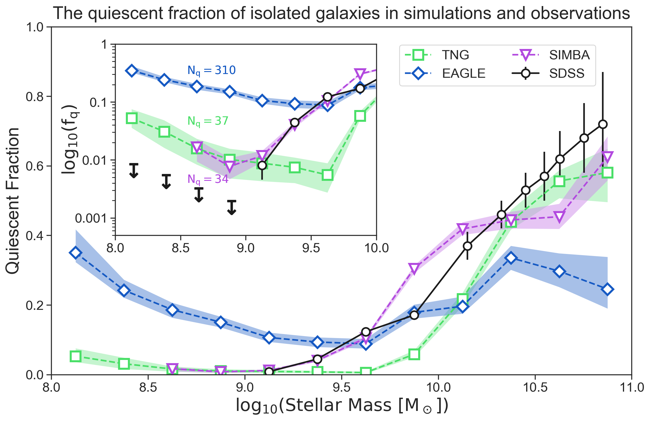
Figure 4: The median quiescent fractions of isolated galaxies as a function of stellar mass for SDSS (black circles), Illustris-TNG (green squares), EAGLE (blue diamonds), and SIMBA (purple triangles). The quiescent fractions for the simulations are the medians of 25 randomly placed sightlines around each simulation box. Shaded regions represent the combination of binomial uncertainty on the quiescent fraction and the variance across sightlines for each simulation. Errorbars on the SDSS quiescent fraction are adapted from Geha et al. (2012). Inset: The same data shown in log-scale. Black arrows represent one-sigma upper limits for the SDSS data in bins where the number of isolated, quiescent galaxies is zero, and the number of isolated, quiescent galaxies ($\mathrm{N_{q}}$) in the lowest mass bin is indicated for each simulation.

4.4 Quenching criteria

As in the observations, simulated galaxies are considered to be quiescent if H$\mathrm{\alpha}$ EW $<2$ Å and $\mathrm{D_{n}4000}$ $>0.6+0.1\log_{10}(\mathrm{M_{*}}/\mathrm{M_{\odot}})$ (orange shaded region in Figure 2). Because $\mathrm{D_{n}4000}$ probes luminosity-weighted stellar age of a galaxy, it is difficult to make a corresponding selection in SFR space, as highlighted by the color-coding of galaxies in Figure 2.

The star forming and quiescent contours shown in Figure 1 can overlap because the $\mathrm{D_{n}4000}$ criterion is mass-dependent for each galaxy. Measuring $\mathrm{D_{n}4000}$ from the realistically-noisy synthetic spectra is crucial to accurately match the sample selection from observations.

4.5 Volume correction

To calculate the quiescent fraction $f_{q}$, we weight each galaxy by the inverse of the total survey volume over which it could be observed given the SDSS spectroscopic magnitude limit ($1/\mathrm{V_{max}}$).

The quiescent fraction of isolated galaxies is then

$$f_{\mathrm{q}}=\frac{\sum\limits^{N_{\mathrm{q}}}_{i=1}1/V_{\mathrm{max},i}}{\sum\limits^{N_{\mathrm{q}}+N_{\mathrm{SF}}}_{i=1}1/V_{\mathrm{max},i}},$$ (1)

where $\mathrm{N_{q}}$ and $\mathrm{N_{SF}}$ are the number of quiescent and star forming galaxies in isolation in each mass bin, respectively.

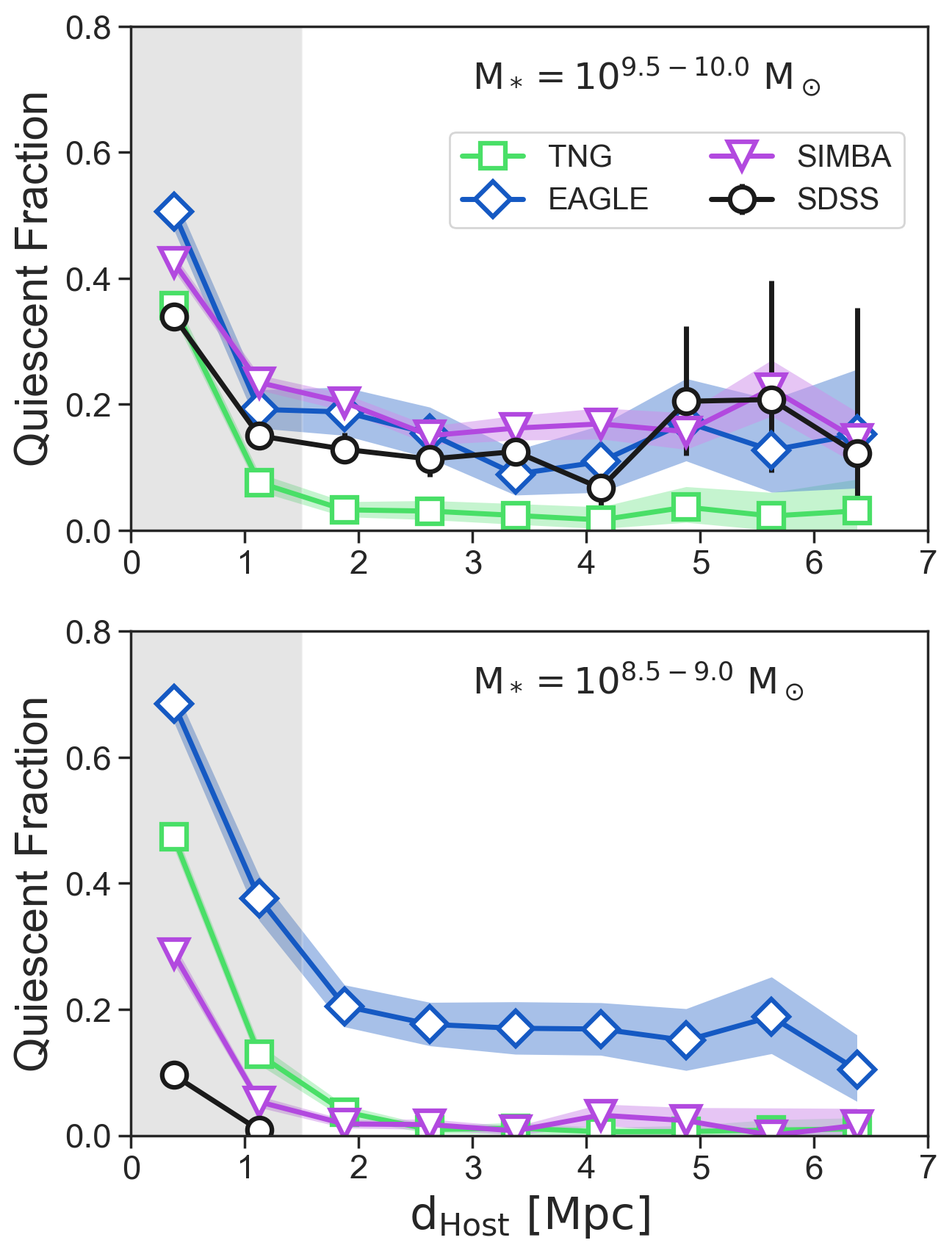
Figure 5: The quiescent fraction of galaxies as function of $\mathrm{d}_{\mathrm{{host}}}$ in two mass bins. The upper panel shows the observed distribution of galaxies with $\mathrm{M_{*}}=10^{9.5-10.0}\ \mathrm{M_{\odot}}$, and the lower panel shows $\mathrm{M_{*}}=10^{8.5-9.0}\ \mathrm{M_{\odot}}$. The gray region indicates $\mathrm{d}_{\mathrm{{host}}}$$<1.5$ Mpc, corresponding to non-isolated galaxies.

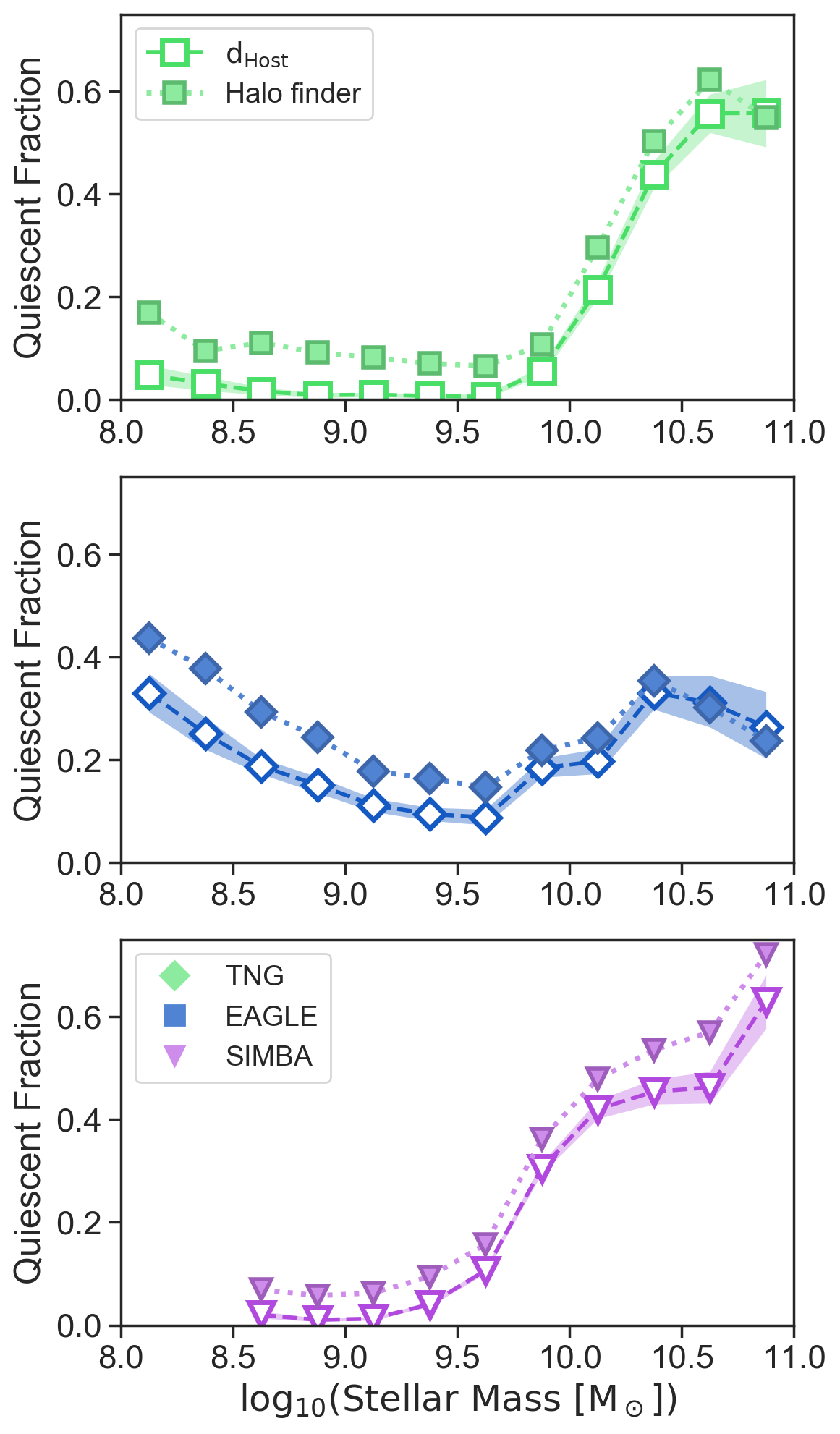
Figure 6: The effects of using a halo finder (filled-color) vs $\mathrm{d}_{\mathrm{{host}}}$ (open-face) to select isolated galaxies on the resultant quiescent fractions in TNG (top), EAGLE (middle), and SIMBA (lower panel). In all three simulations, using the halo finder leads to higher quiescent fractions when compared to $\mathrm{d}_{\mathrm{{host}}}$, driven by the criterion’s more restrictive nature.

5 The Quiescent Fraction of Isolated Galaxies

In Section 5.1, we compare the quiescent fraction of isolated galaxies from each simulation to observations from SDSS. In Section 5.2, Section 5.3 and Section 5.4 we discuss the effects of simulation resolution, observationally-biased stellar mass, and finite aperture on the quiescent fraction, respectively.

5.1 Comparing between simulations and observations

In Figure 4, we show the median isolated quiescent fractions for each simulation from 25 randomly placed sightlines (blue, green and purple points, dashed lines), as compared to SDSS (black circles, solid line).

At intermediate stellar masses ($\mathrm{M_{*}}=10^{9.5-10.5}\ \mathrm{M_{\odot}}$), the simulations all show the quiescent fraction decreasing with decreasing stellar mass, qualitatively reproducing the isolated quenching threshold seen in SDSS (Geha et al., 2012). In observations, this is thought to be driven by the waning efficiency of internal feedback mechanisms. The threshold for TNG galaxies appears to be at a higher stellar mass than is seen in observations, while EAGLE’s quiescent fraction appears to depend less strongly on stellar mass in this regime.

Unlike the observations, all three simulations have non-zero quiescent fractions below $\mathrm{M_{\odot}}=10^{9}\ \mathrm{M_{*}}$ (Figure 4, inset). For both SIMBA and TNG the quiescent fraction, though non-zero, remains small, with $f_{q}\sim 0.01$ at $\mathrm{M_{\odot}}=10^{9}\ \mathrm{M_{*}}$. Overproduction of quiescent galaxies in EAGLE is more pronounced.

We examine the distribution of quiescent galaxies as a function of environment in two mass bins just above and below the observed quenching threshold for isolated galaxies ($10^{8.5-9.0}$ and $10^{9.5-10.0}\ \mathrm{M_{*}}$) in Figure 5. At intermediate stellar masses (upper panel), EAGLE and SIMBA are a good qualitative match to observations, with low quiescent fractions for isolated galaxies and no environmental dependence in the isolated regime. TNG lies below the SDSS observations, with an average $f_{q}\sim 0.05$ beyond $\mathrm{d}_{\mathrm{{host}}}$ $=1.5$ Mpc. At lower stellar masses (lower panel), EAGLE’s over-production of quiescent galaxies in all environments is more pronounced, while SIMBA and TNG are in better agreement, with a near absence of quiescent galaxies beyond $\mathrm{d}_{\mathrm{{host}}}$ $=1.5$ Mpc.

In general, the rapid increase of $f_{q}$ at $\mathrm{d}_{\mathrm{{host}}}$ $<1.5$ Mpc is in qualitative agreement with observations. However, it is notable that all three simulations also overproduce low mass, non-isolated quiescent galaxies, at a many sigma tension given the derived errors. Feedback models for satellite galaxies are often tuned to reproduce galaxies in the Local Group. The SAGA Survey (Mao et al., 2020) recently showed that the Local Group satellites may be over-quenched relative to those around more typical MW-mass galaxies, which may be driving this tension.

In Figure 6, we show how the observed isolated quiescent fraction changes with different definitions of “isolation”. For each simulation, we compare $f_{q}$ derived using $\mathrm{d}_{\mathrm{{host}}}$ and $f_{q}$ from each simulation’s halo finder. In each case, the halo finder produces a larger quiescent fraction (with the exception of $\mathrm{M_{*}}>10^{10.5}\ \mathrm{M_{\odot}}$ in TNG and EAGLE). This effect varies as a function of stellar mass (as well as halo finder used), and highlights the differences between selecting a sample of central galaxies versus isolated galaxies.

5.2 Resolution effects

All three cosmological simulations used in this work have multiple runs at varying resolutions. SIMBA and EAGLE both have smaller boxes with higher resolution and we use these boxes to test our results specifically with respect to resolution. While we do not use the higher resolution version of TNG (TNG50) we note that the effect of resolution on the colors and color bimodality of galaxies is described in Nelson et al. (2018). They argue that the main effect of resolution on galaxy colors is in using purely the stellar particles to derive a star formation history. While we avoid this effect by including instantaneous SFR in the SFHs used to generate our spectra (to reflect the most recent star formation), future work should address explicitly the resolution convergence properties of TNG for the quiescent fractions of low mass galaxies.

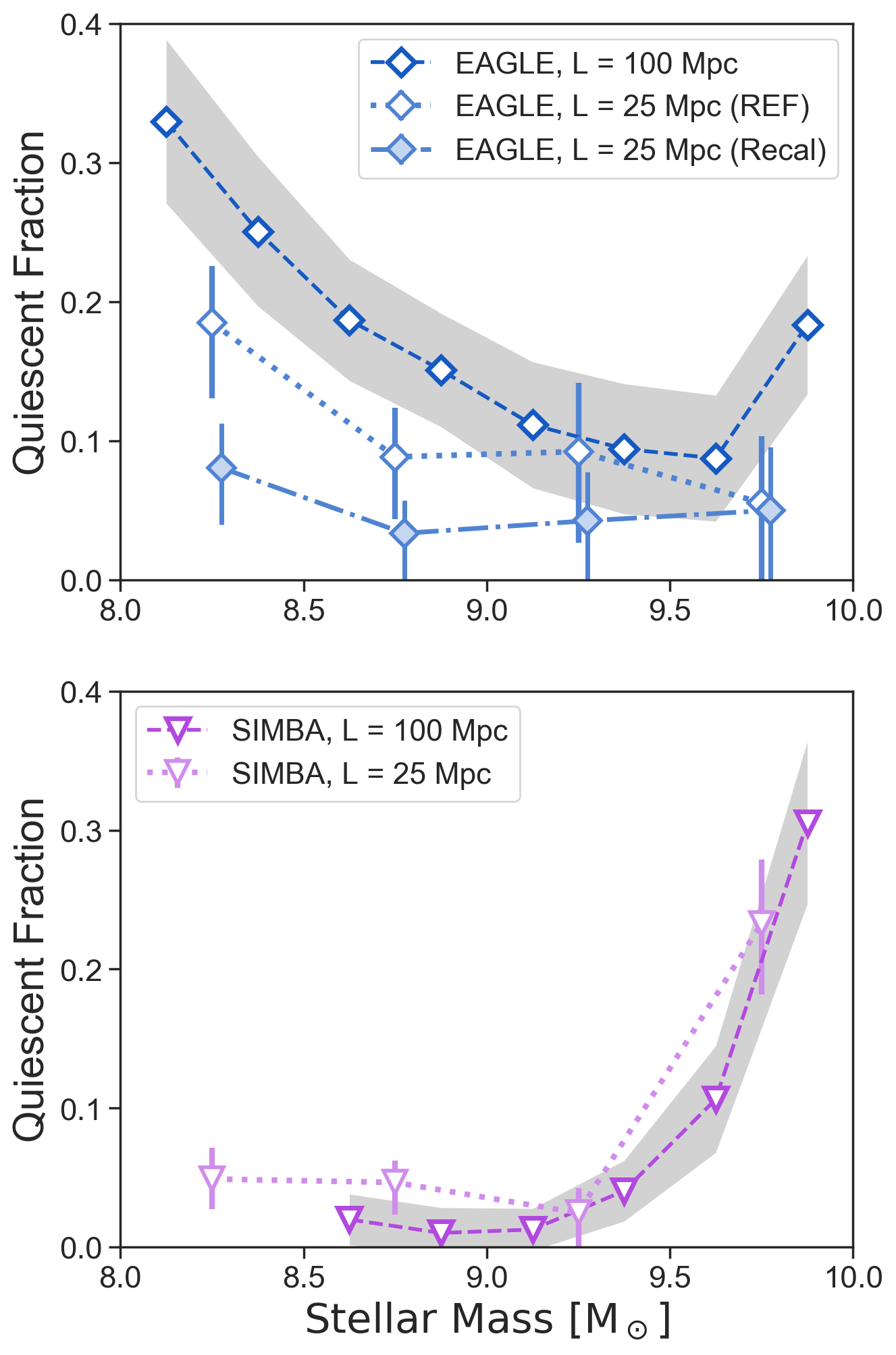
Figure 7: The effects of resolution on the isolated quiescent fraction in EAGLE (upper panel) and SIMBA (lower panel). In both panels, dashed lines show the fiducial quiescent fractions from the large volume, while dotted or dot-dashed lines show the quiescent fractions measured from the higher resolution (25 Mpc)³ volumes. The gray shaded regions represent the maximum variation due to cosmic variance when considering (30 Mpc)³ sub-volumes from each large volume simulation. In the upper panel, data from the two high resolution simulations are offset horizontally so that the errorbars may be distinguished.

In Figure 7 we show the quiescent fraction as a function of stellar mass for the SIMBA and EAGLE higher resolution boxes (light colors, dot and dot-dashed lines) and compare those to the default box and resolution from Figure 4 (dark colors, dashed lines). Because the high-resolution boxes are much smaller in volume, we determine the effect from cosmic variance on the quiescent fraction. To do so, we recompute the quiescent fraction for subboxes of 30Mpc on a side from our default simulation boxes and show the full range of recovered quiescent fractions with the grey shaded regions in each panel. Due to the smaller total number of galaxies, we also use wider mass bins to calculate the quiescent fraction.

For the EAGLE simulations we specifically compare to two boxes of 25Mpc on a side, run using the “Reference” (REF) version of the code (identical to the 100Mpc box), and using the “Recal” version of the code which is re-calibrated at this higher resolution of $m_{\rm DM}=1.21\times 10^{6}\ \mathrm{M_{\odot}}$ and $m_{\rm gas}=2.26\times 10^{5}\ \mathrm{M_{\odot}}$ to counterbalance resolution effects on the subgrid physics (see Schaye et al., 2015; Schaller et al., 2015, for a complete argument and description of the re-calibration, and a comparison of the different versions).

The quiescent fraction of the REF high-resolution box is slightly suppressed compared to that for the large box, falling below what can be explained by cosmic variance alone (gray shading) for the lowest masses. The re-calibrated high-resolution box (RECAL) are further suppressed relative to both the fiducial and REF boxes, and this effect is most extreme at the lowest stellar masses. Schaye et al. (2015) argue that re-calibrating at different resolutions is most appropriate, as (un)physical effects of resolution may be hard to trace. Of the three EAGLE runs examined here, the RECAL box produces the fewest number of quiescent galaxies below $\mathrm{M_{*}}=10^{9}\ \mathrm{M_{\odot}}$, and even agrees with a quiescent fraction of $f_{q}=0$ within the uncertainties for three of the four stellar mass bins. The recalibrated high-resolution EAGLE box is therefore in closest agreement with the observations, though $f_{q}$ does not show the same strong dependence on stellar mass in the mass range $\mathrm{M_{*}}=10^{9-10}\ \mathrm{M_{\odot}}$ that is observed in SDSS. Additionally, both high resolution boxes still show an overabundance of low mass quiescent galaxies in isolation.

For SIMBA the quiescent fraction of low mass galaxies increases slightly at higher resolution, which is run with identical physics to the larger-scale box. We find that the high-resolution box agrees with the fiducial run, with a quiescent fraction that is slightly elevated relative to the fiducial run at $\mathrm{M_{*}}=10^{8.5-9.0}\ \mathrm{M_{\odot}}$. Improved resolution allows for the measurement of the quiescent fraction down to slightly lower stellar masses, which we find to be $f_{q}\sim 0.06$. This is still in tension with SDSS, where no quiescent galaxies are observed in isolation below $\mathrm{M_{*}}=10^{9}\ \mathrm{M_{\odot}}$.

We highlight that the effects of resolution, as exemplified by these case studies, are not uniform across simulations and can increase or decrease the quiescent galaxy fraction.

5.3 Stellar mass

In earlier work, Munshi et al. (2013) found that the stellar masses measured for simulated galaxies with a combination of synthetic Petrosian magnitudes and Bell & de Jong (2001) mass to light ($M/L$) ratios underestimate the true stellar mass by about 50%. This underestimate varied only slightly as a function of mass. Similarly, Leja et al. (2019) have shown that stellar masses inferred from SED modelling with non-parametric SFHs are roughly $\sim 0.2$ dex larger than those obtained under the assumption of an exponentially declining SFH.

We confirm the approximate magnitude of this effect using the $g-r$ color-based approximation for stellar mass from Mao et al. (2020), which produces stellar masses that underestimate the true stellar masses by $\sim 0.3$ dex. In addition to shifting the quenching threshold to lower stellar masses, accounting for systemic error in the measurement of stellar mass leads to a softening of the slope of the quiescent fraction.

5.4 Aperture effects

Our fiducial mock galaxy spectra are based on galaxy properties and star formation histories calculated using all the star and gas elements considered to be part of a simulated galaxy’s subhalo. In comparison, observations of galaxies in SDSS are aperture-limited. There are two SDSS apertures that are important for our results: the photometric aperture and the spectroscopic fiber aperture. The first roughly correspond to with what is considered the size of a galaxy and is relevant for the stellar masses used in this work, and the second for the $\mathrm{D_{n}4000}$ and H$\mathrm{\alpha}$ EW measurements.

With respect to “galaxy size”-aperture effects: previous work using the EAGLE and TNG simulations have found that these aperture effects are significant for high-mass ($\mathrm{M_{*}}\gtrsim 10^{11}\ \mathrm{M_{\odot}}$) galaxies but negligible for lower mass galaxies (Schaye et al., 2015; Donnari et al., 2020a), and we reach similar conclusions when comparing stellar masses in the full subhalo and within a 30 kpc aperture for TNG. Therefore, we conclude that aperture effects are likely insignificant for stellar masses, in particular when compared to other uncertainties as discussed in the previous section.

The aperture of the SDSS spectroscopic fiber typically covers a few kpc in the central region of a galaxy. This means that aperture effects again, are crucial to take into account at higher masses, but can be small for low mass galaxies as there the SDSS fiber aperture may cover a significant fraction of the galaxy. We have checked the differences in $\mathrm{D_{n}4000}$ and H$\mathrm{\alpha}$ EW when only considering the central $r<2$ kpc region of each galaxy. While H$\mathrm{\alpha}$ EW is more variable as a function of aperture (driven by changes in the amount of continuum contained within the aperture), galaxies do not significantly shift in or out of the quiescent region (which is based on both H$\mathrm{\alpha}$ EW and $\mathrm{D_{n}4000}$). In particular, we find only small differences in the quiescent fractions for low mass galaxies, which shift upwards by $\sim 10\%$.

For some observed galaxies the SDSS fiber may have been centered on an off-center bright (star-forming) region. With smaller (lower-mass) galaxies this possibility diminishes purely due to the fact that more of the total galaxy fits within the fiber aperture. Moreover, this is more likely to happen in actively star-forming galaxies, and as we purely use the spectral indices to classify galaxies as star-forming or quiescent, off-center fiber positioning is unlikely to affect our results.

6 Quenching mechanisms in simulations

6.1 Comparison to previous work

Our work is not the first to compare populations of quiescent galaxies from simulations to observations, though we are the first to compare three large volume simulations to observations in a fully consistent manner. Here, we review past studies evaluating the quiescent populations of each simulation.

6.1.1 EAGLE

The quiescent fraction of galaxies in the EAGLE simulations have been discussed in a multitude of papers, using a variety of galaxy subsamples, and of definitions and tracers of the quiescent fraction. Schaye et al. (2015) find that the passive fraction for all galaxies defined based on specific star formation rates (sSFR; SFR/$M_{\star}$) is in reasonably good agreement with results from GAMA (Bauer et al., 2013) and SDSS (Moustakas et al., 2013), although these observational results use slightly different criteria. The threshold where the galaxy population goes from predominantly blue and star-forming to predominantly red and quiescent is found to be at slightly higher stellar mass in EAGLE than for observed low-redshift datasets (Schaye et al., 2015; Trayford et al., 2015). Furlong et al. (2015); Trayford et al. (2015, 2017) show that the apparent larger quiescent fraction at the low mass end is largely due to resolution effects as low mass low-SFR galaxies have very few star-forming gas particles, and show that the recalibrated higher resolution box (Recal-25) agrees with observations.

We agree with their results that the recalibrated high-resolution box improves the quiescent fraction compared to the observations (see Figure 7 and Section 5.2). Nevertheless, we still find that EAGLE produces a higher quiescent fraction for low mass galaxies than is observed in SDSS. It is noteworthy that EAGLE has a particularly high fraction of low mass galaxies that are classified as quiescent but do have current star formation at very low rates. This gives credence to the possibility that the SFR of these galaxies is poorly resolved and that these galaxies are misclassified as quiescent. However, our quiescent definition requires both low H$\mathrm{\alpha}$ and high $\mathrm{D_{n}4000}$. While the H$\mathrm{\alpha}$ can be affected by these resolution effects, the $\mathrm{D_{n}4000}$ is based on the stellar continuum, and probes a longer timescale. Our quiescent fraction may therefore be less dependent on resolution than for a purely H$\mathrm{\alpha}$-based definition.

At higher masses the quiescent fraction we find for EAGLE seem particularly low compared to earlier work based on SFR or sSFR. However, Trayford et al. (2017) show the similar results for $\mathrm{D_{n}4000}$-defined quiescent fractions, and in addition show that dust can affect the discrepancy: when including dust the passive fraction in EAGLE based on a cut of $\mathrm{D_{n}4000}$ $>1.8$ is 35% reduced compared to results from SDSS for galaxies in the mass range $10^{10}\ M_{\odot}<M_{*}<10^{11}\ M_{\odot}$, while without including dust this discrepancy increases to 70% (Trayford et al., 2017). These discrepancies are larger than what we find in this work and may be because our stellar mass-dependent $\mathrm{D_{n}4000}$-based definition of quiescence, which is identical to the one used for the SDSS sample, reaches a lower value at similar masses.

6.1.2 Illustris-TNG

Donnari et al. (2020a) and Donnari et al. (2020b) provide an in-depth exploration of the quenched galaxy fraction in TNG, exploring the effects of aperture, quenching definition, SFR timescale, environmental mis-identification, and incompleteness on the quenched fraction. While they focus on galaxies with $\mathrm{M_{*}}>10^{9}\ \mathrm{M_{\odot}}$ and use SFR or SFS-based definitions of quiescence, we nonetheless find their fiducial quiescent fraction to be in excellent qualitative agreement with our results, specifically the existence of a quenching threshold just above $\mathrm{M_{*}}=10^{10}\ \mathrm{M_{\odot}}$, a small population of isolated (central) galaxies which are quiescent below $\mathrm{M_{*}}=10^{9.5}\ \mathrm{M_{\odot}}$, and a rapid increase in the number of quiescent galaxies from $\mathrm{M_{*}}=10^{10-11}\ \mathrm{M_{\odot}}$.

Donnari et al. (2019) describe the galaxy star forming sequence and the quenched fraction using different definitions and tracers for TNG100. They find that both a UVJ-selected quenched fraction and a distance from the star forming sequence-selected quenched fraction agrees reasonably well with observations, although they use a different UVJ selection for TNG than for the observations they compare to (from Muzzin et al., 2013).

In a by eye comparison, our TNG quiescent fractions (defined based on $\mathrm{D_{n}4000}$ and H$\mathrm{\alpha}$) are overall lower than the UVJ-and-SFS-based quenched fraction from Donnari et al. (2019), in particular at the lower-mass end. A similar difference can be found between the UVJ-selected (Muzzin et al., 2013) and $\mathrm{D_{n}4000}$ and H$\mathrm{\alpha}$-selected (Geha et al., 2012) observed quiescent fractions at $M_{\star}<10^{10}\ M_{\odot}$. As it is unlikely that low mass star-forming galaxies move into the UVJ selection region due to dust, this suggests that the these low mass systems are predominantly red, but still exhibit some low (relatively recent) star formation which can be traced by their $\mathrm{D_{n}4000}$ and/or H$\mathrm{\alpha}$EW.

6.1.3 SIMBA

Davé et al. (2019) have compared the specific star formation rates of SIMBA galaxies to observations from the GALEX-SDSS-WISE Legacy Catalog (Salim et al., 2016, 2018) and found good agreement, which is also consistent with our findings of very good agreement between the quiescent fraction from SIMBA and that observed in SDSS.

Davé et al. (2019) also suggest that the few low mass quiescent galaxies are in fact satellites misclassified by the FOF-based halo finder. Additionally Christiansen et al. (2019); Borrow et al. (2020) show that jet feedback from AGN in SIMBA can influence large regions around the AGN host galaxy and can entrain gas and influence gas in nearby galaxies. The SIMBA 100 Mpc box contains a massive cluster ($\mathrm{M_{*}}\sim 10^{15}\ \mathrm{M_{\odot}}$) and the high-resolution 25 Mpc box also has an anomalously large central halo. However, we confirm that in both boxes, the majority of the quiescent galaxies we select are at least 2 Mpc away from the cluster or most massive halo center, and most are more than 5 Mpc away. Our results suggest that there may be additional effects driving the non-zero quiescent fraction at low mass (see Figure 5, lower panel).

Low mass, quiescent galaxies in SIMBA are also found to be over-sized compared to their star forming counterparts (Davé et al., 2019). However, this should lead to a higher fraction of quiescent galaxies removed from the survey due to the SDSS surface brightness limits. Fixing this issue would therefore only increase the population of low mass, quiescent galaxies in SIMBA.

6.2 Quenching mechanisms of low mass, isolated galaxies in simulations

Given the observed over-abundance of quiescent galaxies at low mass in the simulations, we consider what feedback mechanisms might drive quenching in these systems.

Black holes: some of the low mass galaxies in our sample will contain black holes (almost all galaxies above $\mathrm{M_{*}}=10^{9}\ \mathrm{M_{\odot}}$ in TNG and EAGLE, and above $\mathrm{M_{*}}=10^{9.5}\ \mathrm{M_{\odot}}$ in SIMBA). Feedback from central supermassive black holes is often thought to be able to quench galaxies, and possible important in keeping galaxies quiescent (e.g., Somerville & Davé, 2015, recent discussions include Chen et al., 2020; Terrazas et al., 2016, 2020). However, in the models the black hole feedback often becomes effective only at certain black hole masses (McAlpine et al., 2017; Bower et al., 2017; Weinberger et al., 2018; Thomas et al., 2019; Terrazas et al., 2020; Habouzit et al., 2020), which are not reached in low mass galaxies. Moreover, not all of the low mass galaxies in these simulations will host black holes (especially at $\mathrm{M_{*}}<10^{9}\ \mathrm{M_{\odot}}$), so while black hole feedback could play some role, it is unlikely to the exclusive driver the quenching of the lowest mass galaxies in each simulation.

Star formation feedback: Feedback from star formation is generally thought to reduce the efficiency of galaxy formation at the lower mass end (Somerville & Davé, 2015; Schaller et al., 2015; Schaye et al., 2015; Pillepich et al., 2018b; Davé et al., 2019). Outflows from star formation feedback can temporarily expel large amounts of gas and decrease the gas density of galaxies. This is commonly seen in higher resolution simulations of lower mass galaxies (halo masses $\lesssim 10^{10}\ M_{\odot}$ Wright et al., 2019; Wheeler et al., 2015, 2019; Rey et al., 2020). These effects may result in temporary quiescence, but it is unclear if supernovae are capable of removing enough gas to fully quench galaxies at $\mathrm{M_{*}}\sim 10^{9}\ \mathrm{M_{\odot}}$. Temporarily quiescent low mass galaxies may however, compose part of our quiescent low mass galaxy samples. In large-scale simulations used in this work, the effectiveness of stellar feedback is likely also affected by resolution at the lowest mass end, and the effects of feedback and resolution may be hard to disentangle.

Splashbacks: galaxies moving through larger halos can have their gas stripped away, reducing star formation. Splashback galaxies can be found up to $\sim 3\mathrm{R_{vir}}$ (see e.g., Diemer, 2020) from their true host galaxy, making misidentification possible. However, our $\mathrm{d}_{\mathrm{{host}}}$ isolation criterion is more restrictive than the halo finders (see Figure 6), making it unlikely that more than a small fraction of the isolated quenched galaxies observed in each simulation are splashbacks.

Outflows from nearby massive galaxies: Borrow et al., 2020 and Wright et al., 2019 show that the gas of low mass galaxies (both satellites and low mass centrals) can be stripped or entrained by jets and AGN outflows from more massive halos. While many of the observed isolated galaxies lie many virial radii from any massive halos, this gas removal effect could contribute to the elevated quenched fractions seen in the simulations.

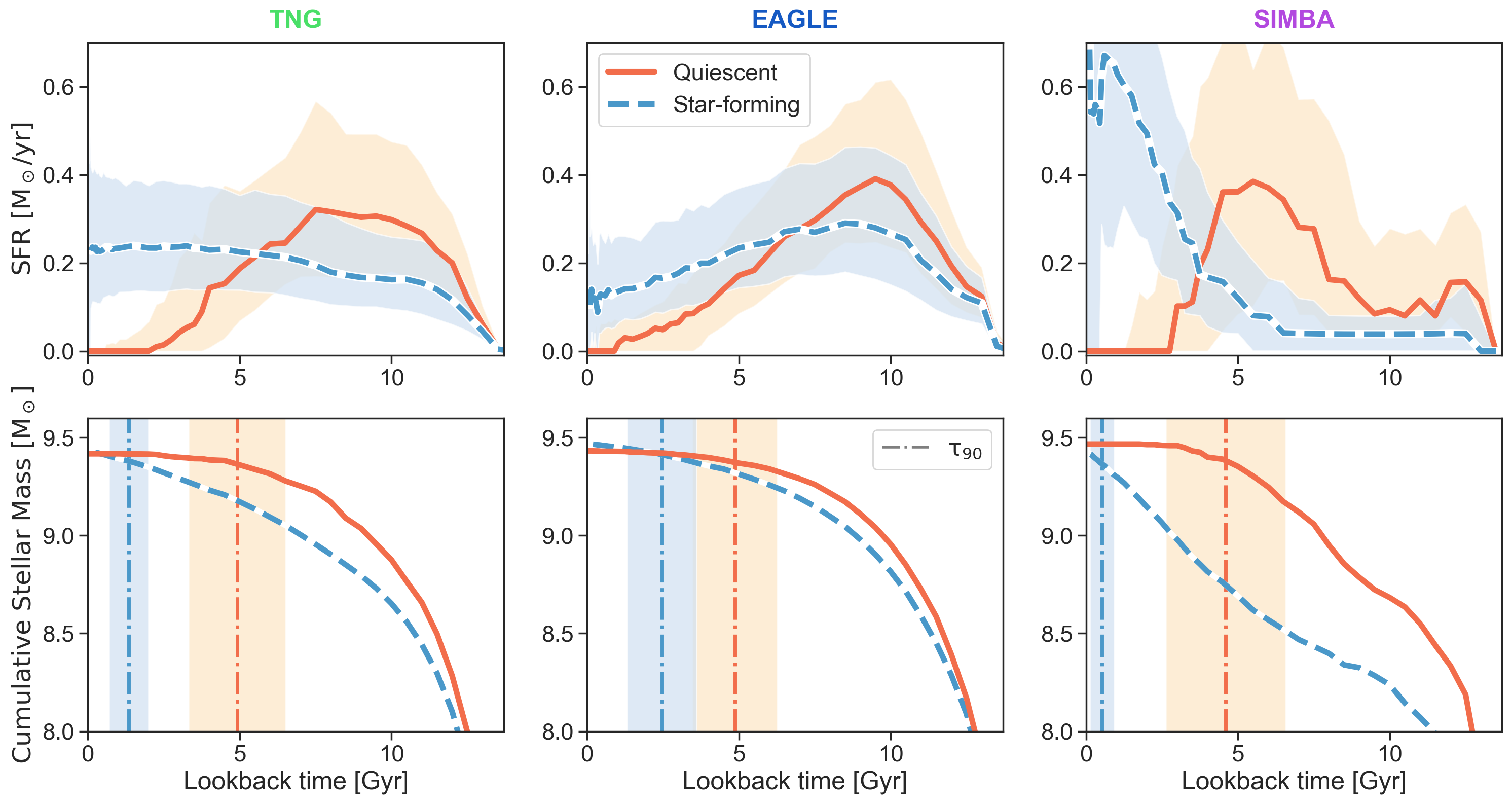
Figure 8: Top row: The median star formation histories of low mass ($\mathrm{M_{*}}=10^{9.0-9.5}\ \mathrm{M_{\odot}}$), isolated galaxies in each simulation, split into star forming (blue, dashed) and quiescent (orange, solid), using the $\mathrm{D_{n}4000}$-H$\mathrm{\alpha}$ EW criteria at $z=0$. Shaded regions encompass the 20-80^th percentile of each distribution.
Bottom row: The median cumulative stellar mass as a function of lookback time for the star forming and quiescent samples of isolated galaxies at low mass in each simulation. Vertical dot-dashed lines show the average time at which 90% of a galaxy’s stellar mass had formed ($\tau_{90}$). Though the star formation histories of quiescent galaxies vary across the three simulations, the average quenching timescales derived for the three populations are effectively identical ($\tau_{90}\sim 5$ Gyr).

7 Star Formation Histories of Quiescent Galaxies

By forward modelling simulated galaxies into observational space, we gain the ability to look back at the “true” properties of observationally-selected galaxies. One of the most informative properties of a galaxy is its star formation history. For each simulated galaxy, we are able to compare the observed properties back to the biases inherent in the recovery of star formation histories from real data.

In Figure 8 (upper row), we show the median star formation histories of low mass ($\mathrm{M_{*}}=10^{9.0-9.5}\ \mathrm{M_{\odot}}$) isolated galaxies observed as star-forming (blue dashed lines) and quiescent (orange solid lines) at $z=0$ in each simulation. The shape of the median star formation histories in each simulation varies significantly. Low mass star forming galaxies in SIMBA show late-time rising star formation histories, while the same galaxies in TNG have approximately flat star formation histories, both in clear contrast with their quiescent counterparts.

In EAGLE, the star formation histories are declining at late times for both the star forming and quiescent populations, and in fact a significant fraction of the low mass quiescent galaxies appear to be forming stars at very low rates at late times. This may be connected to the relatively low scatter in the EAGLE galaxy star-forming sequence (see Hahn et al., 2019) and in the EAGLE star formation histories (Iyer et al., 2020). In particular, the declining and low star formation rates for EAGLE’s low mass galaxies may be connected to the relatively high quiescent fraction that we find using the $\mathrm{D_{n}4000}$ and H$\mathrm{\alpha}$ EW selection. Figure 2 illustrates that of the three simulations in our sample, EAGLE has a notably large fraction of low mass, low-SFR galaxies that are borderline star-forming when considering their specific star formation rates, but have such low SFR that they are classified as quiescent when using the $\mathrm{D_{n}4000}$ and H$\mathrm{\alpha}$ EW measurements.

In the bottom row of Figure 8 we show the median cumulative stellar mass as a function of lookback time for the same star forming and quiescent samples. The vertical dot-dashed lines show the average time at which quiescent and star-forming galaxies formed 90% of their stellar mass (Skillman et al., 2017; Weisz et al., 2015). Despite the apparent variation in the late time star formation histories of the quiescent populations observed in each simulation, $\tau_{90}$ is nearly identical: $\tau_{90,\mathrm{TNG}}=4.9\pm 1.6$ Gyr, $\tau_{90,\mathrm{EAGLE}}=4.9\pm 1.4$ Gyr, and $\tau_{90,\mathrm{SIMBA}}=4.6\pm 2.0$ Gyr. The measurement of $\tau_{90}\sim 5$ Gyr for low mass quiescent galaxies in isolation is a testable prediction for the observational sample and should provide insight into the timescale of feedback mechanisms which drive quenching in low mass galaxies.

Of the galaxies observed as quiescent, a subset in each simulation have non-zero instantaneous star formation rates at $z=0$ (approximately 50% of low mass galaxies in TNG and EAGLE, and 20% in SIMBA). The empirical definition of quiescence used throughout this work (based on $\mathrm{D_{n}4000}$ and H$\mathrm{\alpha}$ EW) selects galaxies with a range of evolutionary histories and $z=0$ properties. We find that the SFR=0 galaxies do not separate out cleanly in $\mathrm{D_{n}4000}$  -  H$\mathrm{\alpha}$ EW space (highlighted in Figure 2). In order to select a totally quiescent sample of galaxies, additional probes of SFR would be required. Characterizing exactly how much ongoing star formation a galaxy can experience while still being selected by a given definition of quiescence will help inform the selection of appropriate quenching criteria (e.g., UVJ vs SFR vs $\mathrm{D_{n}4000}$) going forward.

In future work, we will constrain the average quenching time for observed quiescent galaxies in isolation via SED fitting, and apply the same process to the synthetic spectra. Applying the same SED fitting methods to the synthetic data is critical, as the observed differences in the late time star formation history may only be recoverable above a certain threshold of data quality (e.g., spectrum SNR, photometric wavelength coverage).

8 Conclusions

In this paper, we have produced mock SDSS-like surveys from three large volume hydrodynamic simulations (Illustris-TNG, EAGLE, and SIMBA) from which we measured the quiescent fraction of isolated galaxies and compared back to extant constraints from the local universe (Geha et al., 2012). We find that:

1. The three simulations examined in this work, when transformed into observational space using an identical methodology, produce three different dependencies of the quiescent fraction on stellar mass. Above $\mathrm{M_{*}}=10^{9.5}\ \mathrm{M_{\odot}}$, all three simulations qualitatively reproduce the declining quiescent fraction with decreasing stellar mass observed in SDSS.

2. All three simulations have non-zero quiescent fractions below $\mathrm{M_{*}}=10^{9.0}\ \mathrm{M_{\odot}}$, in contrast to observations of the SDSS volume. This suggests that current models of feedback in the low stellar mass regime are too efficient.

3. Our empirical definition of quiescence selects low mass galaxies with a range of star formation histories when viewed over longer (many Gyr) timescales. However, these populations all show similar quenching timescales ($\tau_{90}\sim 5$ Gyr), which can be compared back to observations. Understanding how sensitive a particular definition of quenching is to formation history can inform future population studies.

4. Measuring the quiescent fraction in a higher resolution box does not fully resolve the overabundance of quiescent galaxies below $\mathrm{M_{*}}=10^{9.0}\ \mathrm{M_{\odot}}$. In fact, improved resolution can lead to either a significant decrease or slight increase in the measured quiescent fraction, depending on the simulation. While the low mass quiescent fraction is not converged in the large-scale simulations, the discrepancy with observations persists at higher resolutions.

The low mass quenching threshold of isolated galaxies represents an observational boundary condition; a stellar mass regime where internal feedback mechanisms become ineffective. Observations of the isolated galaxy quiescent fraction provide a unique probe into the delicate balance of internal feedback mechanisms in low mass galaxies. Understanding how well or poorly modern simulations of galaxy evolution can reproduce this feature is a novel test of feedback prescriptions, but requires the creation of mock observations and surveys to enable appropriate comparisons between the observed universe and simulations.

Our method for producing mock surveys from large volume hydrodynamic simulations can also be applied to zoom-in simulations and semi-analytic models, and adapted to match other surveys and observations. Future work will explore the star formation histories recovered from synthetic observations as compared to those derived from observations, as well as the observed gas properties of simulated galaxies.

The constraining power of the observations we compare to are set by the size of the SDSS volume and the limiting magnitude and surface brightness of the survey. Future wide-field surveys such as the Vera Rubin Observatory’s Large Synoptic Survey Telescope (LSST; Ivezić et al., 2019) and the Dark Energy Survey Instrument (DESI; DESI Collaboration et al., 2016) have the potential to substantially improve our census of the local universe, providing new constraints on the population of low mass, quiescent galaxies in the field.

Making direct comparisons between observations and simulations requires the careful translation from the simulation to observational frame (or vice versa). In doing so, we gain novel insights into the ways that feedback shapes the evolution of galaxies.

References

- Aihara et al. (2011) Aihara, H., Allende Prieto, C., An, D., et al. 2011, ApJS, 193, 29
- Anglés-Alcázar et al. (2017a) Anglés-Alcázar, D., Davé, R., Faucher-Giguère, C.-A., Özel, F., & Hopkins, P. F. 2017a, MNRAS, 464, 2840
- Anglés-Alcázar et al. (2017b) Anglés-Alcázar, D., Faucher-Giguère, C.-A., Kereš, D., et al. 2017b, MNRAS, 470, 4698
- Anglés-Alcázar et al. (2013) Anglés-Alcázar, D., Özel, F., & Davé, R. 2013, ApJ, 770, 5
- Anglés-Alcázar et al. (2015) Anglés-Alcázar, D., Özel, F., Davé, R., et al. 2015, ApJ, 800, 127
- Appleby et al. (2019) Appleby, S., Davé, R., Kraljic, K., Anglés-Alcázar, D., & Narayanan, D. 2019, arXiv e-prints, arXiv:1911.02041
- Astropy Collaboration et al. (2013) Astropy Collaboration, Robitaille, T. P., Tollerud, E. J., et al. 2013, A&A, 558, A33
- Astropy Collaboration et al. (2018) Astropy Collaboration, Price-Whelan, A. M., SipHocz, B. M., et al. 2018, aj, 156, 123
- Baes et al. (2011) Baes, M., Verstappen, J., De Looze, I., et al. 2011, ApJS, 196, 22
- Balogh et al. (1999) Balogh, M. L., Morris, S. L., Yee, H. K. C., Carlberg, R. G., & Ellingson, E. 1999, ApJ, 527, 54
- Bauer et al. (2013) Bauer, A. E., Hopkins, A. M., Gunawardhana, M., et al. 2013, MNRAS, 434, 209
- Bell & de Jong (2001) Bell, E. F., & de Jong, R. S. 2001, ApJ, 550, 212
- Bell et al. (2003) Bell, E. F., McIntosh, D. H., Katz, N., & Weinberg, M. D. 2003, ApJS, 149, 289
- Blanton et al. (2011) Blanton, M. R., Kazin, E., Muna, D., Weaver, B. A., & Price-Whelan, A. 2011, AJ, 142, 31
- Blanton & Moustakas (2009) Blanton, M. R., & Moustakas, J. 2009, ARA&A, 47, 159
- Blanton et al. (2003) Blanton, M. R., Hogg, D. W., Bahcall, N. A., et al. 2003, ApJ, 594, 186
- Borrow et al. (2020) Borrow, J., Anglés-Alcázar, D., & Davé, R. 2020, MNRAS, 491, 6102
- Bower et al. (2017) Bower, R. G., Schaye, J., Frenk, C. S., et al. 2017, MNRAS, 465, 32
- Brammer et al. (2009) Brammer, G. B., Whitaker, K. E., van Dokkum, P. G., et al. 2009, ApJ, 706, L173
- Brinchmann et al. (2004) Brinchmann, J., Charlot, S., White, S. D. M., et al. 2004, MNRAS, 351, 1151
- Byler et al. (2017) Byler, N., Dalcanton, J. J., Conroy, C., & Johnson, B. D. 2017, ApJ, 840, 44
- Camps et al. (2018) Camps, P., Trčka, A., Trayford, J., et al. 2018, ApJS, 234, 20
- Chabrier (2003) Chabrier, G. 2003, PASP, 115, 763
- Charlot & Fall (2000) Charlot, S., & Fall, S. M. 2000, ApJ, 539, 718
- Chen et al. (2020) Chen, Z., Faber, S. M., Koo, D. C., et al. 2020, ApJ, 897, 102
- Choi et al. (2012) Choi, E., Ostriker, J. P., Naab, T., & Johansson, P. H. 2012, ApJ, 754, 125
- Christiansen et al. (2019) Christiansen, J. F., Davé, R., Sorini, D., & Anglés-Alcázar, D. 2019, arXiv e-prints, arXiv:1911.01343
- Conroy & Gunn (2010) Conroy, C., & Gunn, J. E. 2010, ApJ, 712, 833
- Conroy et al. (2009) Conroy, C., Gunn, J. E., & White, M. 2009, ApJ, 699, 486
- Crain et al. (2015) Crain, R. A., Schaye, J., Bower, R. G., et al. 2015, MNRAS, 450, 1937
- Daddi et al. (2007) Daddi, E., Dickinson, M., Morrison, G., et al. 2007, ApJ, 670, 156
- Dalla Vecchia & Schaye (2012) Dalla Vecchia, C., & Schaye, J. 2012, MNRAS, 426, 140
- Davé et al. (2019) Davé, R., Anglés-Alcázar, D., Narayanan, D., et al. 2019, MNRAS, 486, 2827
- Davé et al. (2017) Davé, R., Rafieferantsoa, M. H., Thompson, R. J., & Hopkins, P. F. 2017, MNRAS, 467, 115
- Davé et al. (2016) Davé, R., Thompson, R., & Hopkins, P. F. 2016, MNRAS, 462, 3265
- Davies et al. (2020) Davies, J. J., Crain, R. A., Oppenheimer, B. D., & Schaye, J. 2020, MNRAS, 491, 4462
- Davis et al. (1985) Davis, M., Efstathiou, G., Frenk, C. S., & White, S. D. M. 1985, ApJ, 292, 371
- DESI Collaboration et al. (2016) DESI Collaboration, Aghamousa, A., Aguilar, J., et al. 2016, arXiv e-prints, arXiv:1611.00036
- Dickey et al. (2019) Dickey, C. M., Geha, M., Wetzel, A., & El-Badry, K. 2019, ApJ, 884, 180
- Diemer (2020) Diemer, B. 2020, arXiv e-prints, arXiv:2007.10992
- Donnari et al. (2020a) Donnari, M., Pillepich, A., Nelson, D., et al. 2020a, arXiv e-prints, arXiv:2008.00004
- Donnari et al. (2019) —. 2019, MNRAS, 485, 4817
- Donnari et al. (2020b) Donnari, M., Pillepich, A., Joshi, G. D., et al. 2020b, arXiv e-prints, arXiv:2008.00005
- El-Badry et al. (2016) El-Badry, K., Wetzel, A., Geha, M., et al. 2016, ApJ, 820, 131
- Elbaz et al. (2007) Elbaz, D., Daddi, E., Le Borgne, D., et al. 2007, A&A, 468, 33
- Fillingham et al. (2018) Fillingham, S. P., Cooper, M. C., Boylan-Kolchin, M., et al. 2018, MNRAS, 477, 4491
- Flores Velázquez et al. (2020) Flores Velázquez, J. A., Gurvich, A. B., Faucher-Giguère, C.-A., et al. 2020, arXiv e-prints, arXiv:2008.08582
- Foreman-Mackey et al. (2014) Foreman-Mackey, D., Sick, J., & Johnson, B. 2014, Python-Fsps: Python Bindings to FSPS (v0.1.1), Zenodo
- Foreman-Mackey et al. (2014) Foreman-Mackey, D., Sick, J., & Johnson, B. 2014, Python-Fsps: Python Bindings To Fsps (V0.1.1)
- Furlong et al. (2015) Furlong, M., Bower, R. G., Theuns, T., et al. 2015, MNRAS, 450, 4486
- Geha et al. (2012) Geha, M., Blanton, M. R., Yan, R., & Tinker, J. L. 2012, ApJ, 757, 85
- Genel et al. (2014) Genel, S., Vogelsberger, M., Springel, V., et al. 2014, MNRAS, 445, 175
- Genel et al. (2018) Genel, S., Nelson, D., Pillepich, A., et al. 2018, MNRAS, 474, 3976
- Habouzit et al. (2019) Habouzit, M., Genel, S., Somerville, R. S., et al. 2019, MNRAS, 484, 4413
- Habouzit et al. (2020) Habouzit, M., Li, Y., Somerville, R. S., et al. 2020, arXiv e-prints, arXiv:2006.10094
- Hahn et al. (2019) Hahn, C., Starkenburg, T. K., Choi, E., et al. 2019, ApJ, 872, 160
- Hamilton (1985) Hamilton, D. 1985, ApJ, 297, 371
- Harris et al. (2020) Harris, C. R., Millman, K. J., van der Walt, S. J., et al. 2020, Nature, 585, 357–362
- Hopkins (2015) Hopkins, P. F. 2015, MNRAS, 450, 53
- Hopkins (2017) —. 2017, arXiv e-prints, arXiv:1712.01294
- Hopkins et al. (2014) Hopkins, P. F., Kereš, D., Oñorbe, J., et al. 2014, MNRAS, 445, 581
- Hopkins & Quataert (2011) Hopkins, P. F., & Quataert, E. 2011, MNRAS, 415, 1027
- Hopkins et al. (2018) Hopkins, P. F., Wetzel, A., Kereš, D., et al. 2018, MNRAS, 480, 800
- Hunter (2007) Hunter, J. D. 2007, Computing in Science & Engineering, 9, 90
- Ivezić et al. (2019) Ivezić, Ž., Kahn, S. M., Tyson, J. A., et al. 2019, ApJ, 873, 111
- Iyer et al. (2020) Iyer, K. G., Tacchella, S., Genel, S., et al. 2020, MNRAS, 498, 430
- Katsianis et al. (2020) Katsianis, A., Gonzalez, V., Barrientos, D., et al. 2020, MNRAS, 492, 5592
- Kauffmann et al. (2004) Kauffmann, G., White, S. D. M., Heckman, T. M., et al. 2004, MNRAS, 353, 713
- Kauffmann et al. (2003) Kauffmann, G., Heckman, T. M., White, S. D. M., et al. 2003, MNRAS, 341, 54
- Kennicutt & Evans (2012) Kennicutt, R. C., & Evans, N. J. 2012, ARA&A, 50, 531
- Koudmani et al. (2019) Koudmani, S., Sijacki, D., Bourne, M. A., & Smith, M. C. 2019, MNRAS, 484, 2047
- Leja et al. (2019) Leja, J., Johnson, B. D., Conroy, C., et al. 2019, ApJ, 877, 140
- Li et al. (2019) Li, Y., Habouzit, M., Genel, S., et al. 2019, arXiv e-prints, arXiv:1910.00017
- Mao et al. (2020) Mao, Y.-Y., Geha, M., Wechsler, R. H., et al. 2020, arXiv e-prints, arXiv:2008.12783
- Marinacci et al. (2018) Marinacci, F., Vogelsberger, M., Pakmor, R., et al. 2018, MNRAS, 480, 5113
- McAlpine et al. (2017) McAlpine, S., Bower, R. G., Harrison, C. M., et al. 2017, MNRAS, 468, 3395
- McAlpine et al. (2018) McAlpine, S., Bower, R. G., Rosario, D. J., et al. 2018, MNRAS, 481, 3118
- McAlpine et al. (2016) McAlpine, S., Helly, J. C., Schaller, M., et al. 2016, Astronomy and Computing, 15, 72
- McKinnon et al. (2017) McKinnon, R., Torrey, P., Vogelsberger, M., Hayward, C. C., & Marinacci, F. 2017, MNRAS, 468, 1505
- Moustakas et al. (2006) Moustakas, J., Kennicutt, Robert C., J., & Tremonti, C. A. 2006, ApJ, 642, 775
- Moustakas et al. (2013) Moustakas, J., Coil, A. L., Aird, J., et al. 2013, ApJ, 767, 50
- Munshi et al. (2013) Munshi, F., Governato, F., Brooks, A. M., et al. 2013, ApJ, 766, 56
- Muratov et al. (2015) Muratov, A. L., Kereš, D., Faucher-Giguère, C.-A., et al. 2015, MNRAS, 454, 2691
- Muzzin et al. (2013) Muzzin, A., Marchesini, D., Stefanon, M., et al. 2013, ApJ, 777, 18
- Naab & Ostriker (2017) Naab, T., & Ostriker, J. P. 2017, ARA&A, 55, 59
- Naiman et al. (2018) Naiman, J. P., Pillepich, A., Springel, V., et al. 2018, MNRAS, 477, 1206
- Nelson et al. (2018) Nelson, D., Pillepich, A., Springel, V., et al. 2018, MNRAS, 475, 624
- Noeske et al. (2007) Noeske, K. G., Weiner, B. J., Faber, S. M., et al. 2007, ApJ, 660, L43
- Peng et al. (2010) Peng, Y.-j., Lilly, S. J., Kovač, K., et al. 2010, ApJ, 721, 193
- Penny et al. (2018) Penny, S. J., Masters, K. L., Smethurst, R., et al. 2018, MNRAS, 476, 979
- Pérez & Granger (2007) Pérez, F., & Granger, B. E. 2007, Computing in Science and Engineering, 9, 21
- Pillepich et al. (2018a) Pillepich, A., Nelson, D., Hernquist, L., et al. 2018a, MNRAS, 475, 648
- Pillepich et al. (2018b) Pillepich, A., Springel, V., Nelson, D., et al. 2018b, MNRAS, 473, 4077
- Rey et al. (2020) Rey, M. P., Pontzen, A., Agertz, O., et al. 2020, MNRAS, 497, 1508
- Rodríguez Montero et al. (2019) Rodríguez Montero, F., Davé, R., Wild, V., Anglés-Alcázar, D., & Narayanan, D. 2019, MNRAS, 490, 2139
- Sales et al. (2015) Sales, L. V., Vogelsberger, M., Genel, S., et al. 2015, MNRAS, 447, L6
- Salim et al. (2018) Salim, S., Boquien, M., & Lee, J. C. 2018, ApJ, 859, 11
- Salim et al. (2007) Salim, S., Rich, R. M., Charlot, S., et al. 2007, ApJS, 173, 267
- Salim et al. (2016) Salim, S., Lee, J. C., Janowiecki, S., et al. 2016, ApJS, 227, 2
- Schaller et al. (2015) Schaller, M., Dalla Vecchia, C., Schaye, J., et al. 2015, MNRAS, 454, 2277
- Schaye et al. (2015) Schaye, J., Crain, R. A., Bower, R. G., et al. 2015, MNRAS, 446, 521
- Skillman et al. (2017) Skillman, E. D., Monelli, M., Weisz, D. R., et al. 2017, ApJ, 837, 102
- Somerville & Davé (2015) Somerville, R. S., & Davé, R. 2015, ARA&A, 53, 51
- Sparre et al. (2015) Sparre, M., Hayward, C. C., Springel, V., et al. 2015, MNRAS, 447, 3548
- Speagle et al. (2014) Speagle, J. S., Steinhardt, C. L., Capak, P. L., & Silverman, J. D. 2014, ApJS, 214, 15
- Springel (2005) Springel, V. 2005, MNRAS, 364, 1105
- Springel (2010) —. 2010, ARA&A, 48, 391
- Springel et al. (2001a) Springel, V., White, S. D. M., Tormen, G., & Kauffmann, G. 2001a, MNRAS, 328, 726
- Springel et al. (2001b) Springel, V., Yoshida, N., & White, S. D. M. 2001b, New A, 6, 79
- Springel et al. (2018) Springel, V., Pakmor, R., Pillepich, A., et al. 2018, MNRAS, 475, 676
- Terrazas et al. (2016) Terrazas, B. A., Bell, E. F., Henriques, B. M. B., et al. 2016, ApJ, 830, L12
- Terrazas et al. (2020) Terrazas, B. A., Bell, E. F., Pillepich, A., et al. 2020, MNRAS, 493, 1888
- Thomas et al. (2019) Thomas, N., Davé, R., Anglés-Alcázar, D., & Jarvis, M. 2019, MNRAS, 487, 5764
- Tinker et al. (2011) Tinker, J., Wetzel, A., & Conroy, C. 2011, arXiv e-prints, arXiv:1107.5046
- Torrey et al. (2014) Torrey, P., Vogelsberger, M., Genel, S., et al. 2014, MNRAS, 438, 1985
- Trayford et al. (2015) Trayford, J. W., Theuns, T., Bower, R. G., et al. 2015, MNRAS, 452, 2879
- Trayford et al. (2017) Trayford, J. W., Camps, P., Theuns, T., et al. 2017, MNRAS, 470, 771
- Trčka et al. (2020) Trčka, A., Baes, M., Camps, P., et al. 2020, MNRAS, 494, 2823
- Van Rossum & Drake (2009) Van Rossum, G., & Drake, F. L. 2009, Python 3 Reference Manual (Scotts Valley, CA: CreateSpace)
- Villaume et al. (2015) Villaume, A., Conroy, C., & Johnson, B. D. 2015, ApJ, 806, 82
- Virtanen et al. (2020) Virtanen, P., Gommers, R., Oliphant, T. E., et al. 2020, Nature Methods, 17, 261
- Vogelsberger et al. (2020) Vogelsberger, M., Marinacci, F., Torrey, P., & Puchwein, E. 2020, Nature Reviews Physics, 2, 42
- Vogelsberger et al. (2014) Vogelsberger, M., Genel, S., Springel, V., et al. 2014, MNRAS, 444, 1518
- Weinberger et al. (2017) Weinberger, R., Ehlert, K., Pfrommer, C., Pakmor, R., & Springel, V. 2017, MNRAS, 470, 4530
- Weinberger et al. (2018) Weinberger, R., Springel, V., Pakmor, R., et al. 2018, MNRAS, 479, 4056
- Weisz et al. (2015) Weisz, D. R., Dolphin, A. E., Skillman, E. D., et al. 2015, ApJ, 804, 136
- Wetzel et al. (2012) Wetzel, A. R., Tinker, J. L., & Conroy, C. 2012, MNRAS, 424, 232
- Wetzel et al. (2013) Wetzel, A. R., Tinker, J. L., Conroy, C., & van den Bosch, F. C. 2013, MNRAS, 432, 336
- Wetzel et al. (2015) Wetzel, A. R., Tollerud, E. J., & Weisz, D. R. 2015, ApJ, 808, L27
- Wheeler et al. (2015) Wheeler, C., Oñorbe, J., Bullock, J. S., et al. 2015, MNRAS, 453, 1305
- Wheeler et al. (2019) Wheeler, C., Hopkins, P. F., Pace, A. B., et al. 2019, MNRAS, 490, 4447
- Wright et al. (2019) Wright, A. C., Brooks, A. M., Weisz, D. R., & Christensen, C. R. 2019, MNRAS, 482, 1176
- Yan (2011) Yan, R. 2011, AJ, 142, 153
- Yan & Blanton (2012) Yan, R., & Blanton, M. R. 2012, ApJ, 747, 61
- Yan et al. (2006) Yan, R., Newman, J. A., Faber, S. M., et al. 2006, ApJ, 648, 281
- York et al. (2000) York, D. G., Adelman, J., Anderson, John E., J., et al. 2000, AJ, 120, 1579