Weighing an optically trapped microsphere in thermal equilibrium with air

Abstract

We report a weighing metrology experiment of a single silica microsphere optically trapped and immersed in air. Based on fluctuations about thermal equilibrium, three different mass measurements are investigated, each arising from one of two principle methods. The first method is based on spectral analysis and enables simultaneous extraction of various system parameters. Additionally, the spectral method yields a mass measurement with systematic relative uncertainty of 3.0% in 3 s and statistical relative uncertainty of 0.9% across several trapping laser powers. Parameter values learned from the spectral method serve as input, or a calibration step, for the second method based on the equipartition theorem. The equipartition method gives two additional mass measurements with systematic and statistical relative uncertainties slightly larger than the ones obtained in the spectral method, but over a time interval 10 times shorter. Our mass estimates, which are obtained in a scenario of strong environmental coupling, have uncertainties comparable to ones obtained in force-driven metrology experiments with nanospheres in vacuum. Moreover, knowing the microsphere’s mass accurately and precisely will enable air-based sensing applications.

I Introduction

Optical trapping of nano- and micro-scale objects [1, 2, 3] has become a paradigmatic tool in diverse fields, from micro-manipulation of biological samples [4, 5, 6, 7, 8, 9, 10, 11, 12, 13, 14, 15] to center-of-mass cooling experiments [16, 17, 18] aiming to observe macroscopic quantum effects [19, 20, 21], to metrology experiments [22, 23, 24] with optomechanical sensing applications [25, 26, 27, 28, 29]. In such experiments, a tightly focused laser beam, named the optical tweezer [30, 31, 32], is used to polarize a dielectric particle and harmonically confine it to the beam’s intensity maximum.

It is often desirable to monitor the trapped particle’s position as a function of time, so a position-sensitive detector must be calibrated. Calibrating the detector usually requires knowledge of the trapped particle’s mass [22]. However, $\mathrm{SiO_{2}}$ nano and microspheres, often the object-of-study in levitated optomechanics experiments, do not have a readily-known mass. The Stöber process used to manufacture these particles [33] yields very spherical results with a low dispersion of radius ($\sim 3\%$), but a mass density which can vary in excess of 20% [33, 34]. Calculated with these values, the uncertainty in mass is about 22%. For this reason, recent work has focused on mass metrology of nano and microspheres optically trapped in vacuum using methods of electrostatic levitation [34], oscillation [23], and trapping potential nonlinearities [24], and, most recently a drop-recapture method perfomed in air [35]. The mass uncertainty achieved in each of these experiments is at the level of one to a few percent. Each has unique advantages like no assumptions on particle geometry, and distinct challenges, e.g., control of the particle’s charge, accurate modelling of local potentials (gravitational, electric, or optical), or vacuum capabilities including feedback cooling.

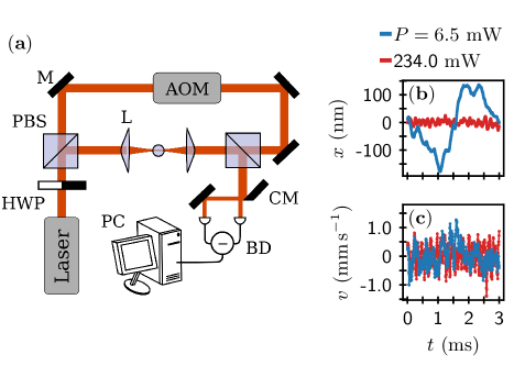
Figure 1: (a) Schematic of the dual beam optical trap and the detection system: (M) dielectric mirror; (HWP) half wave plate; (PBS) polarizing beamsplitter; (AOM) acoustic optical modulator; (L) aspheric lense; (CM) cut mirror; (BD) balanced photodetector; (PC) personal computer. (b) An example position trace at high and low trapping power; (c) An example velocity trace which is computed with an $\rm 8^{th}$-order-accuracy numeric finite difference of the data in (b).

Here, we report on a mass metrology experiment with uncertainty similar to previous work, but performed on a $1.5~{}$\mathrm{\SIUnitSymbolMicro}\mathrm{m}$$ radius $\rm SiO_{2}$ microsphere optically trapped in air [36] at room temperature and pressure. Our experiment employs a dual-beam optical trap [1, 37], sketched in Fig. 1(a) and elaborated upon in Our system remains in thermal equilibrium at all times making for a simple protocol. Moreover, we explore two distinct methodologies leveraging our detector’s high spatiotemporal resolution. In the first spectral method, we fit an average voltage signal power spectral density (PSD) to simultaneously extract parameters which make no assumptions on the physical conditions of the experiment. We then fix conditions known with high accuracy — the air temperature, air viscosity, and particle radius — to compute the harmonic trap strength $k$, microsphere mass density $\rho$, and detector calibration factor $\beta$, as well as the uncertainties and correlations of these parameters. The microsphere mass is similarly calculated by combining fitting and fixed parameters.

In the second equipartition method, we compute the voltage signal and voltage-derivative signal variances from which we deduce the particle mass in two additional ways. Doing so requires a detector with sufficient resolution to observe the particle’s instantaneous velocity, pioneered in  [16, 38]. The equipartition methods additionally require knowledge of either the harmonic trap strength $k$ or calibration factor $\beta$ which must be determined via the spectral method first. The spectral method demands a high volume of data to sufficiently smooth the experimental PSD, and is in that sense slow. The equipartition methods, once an initial spectral calibration is performed, require 10 times less data to achieve similar uncertainty in subsequent mass measurements.

Making precise and fast mass measurements in a system strongly coupled to the environment might have applications in scenarios where either the mass changes with time but temperature is fixed, for instance in heterogeneous nucleation [39, 40], or the mass is fixed but temperature changes, like in Rayleigh-Bénard convection [41, 42].

This Article is organized as follows: first, we review the relevant physics and outline our PSD parameter estimation method in Section II. In Section III we show how the PSD parameters, along with the equipartition theorem, allow us to weigh the microsphere in three different ways. There, we also present the results which we further discussion in Section IV. Finally, we conclude with this work’s significance in section V.

II Power spectral density parameter estimation

The dynamics of the trapped microsphere along the $x$-axis may be modeled by the harmonically bound Langevin equation of motion

$$m\ddot{x}+\gamma\dot{x}+kx=F(t),$$ (1)

where $m=4\pi\rho R^{3}/3$ is the mass of the microsphere with radius $R$ and density $\rho$, $\gamma=6\pi\eta R$ is the Stokes friction coefficient, $\eta$ is the viscosity of air, and $k$ is the trap strength. The stochastic thermal force $F(t)=g\xi(t)$ is assumed to have the form of zero-mean $\langle\xi(t)\rangle=0$, delta-correlated $\langle\xi(t)\xi(t^{\prime})\rangle=\delta(t-t^{\prime})$ white noise with strength $g=\sqrt{2{k}_{\mathrm{B}}T\gamma}$ (according to the fluctuation-dissipation theorem), and in which $T$ is the air temperature, ${k}_{\mathrm{B}}$ is Boltzmann’s constant, and $\langle\cdot\rangle$ denotes ensemble averages over realizations of $\xi$. Writing Eq. (1), in terms of the Fourier transforms $\tilde{x}(\omega)$ and $\tilde{F}(\omega)$ lets one deduce the position PSD $S_{x}(\omega)$ such that $\langle\tilde{x}(\omega)\tilde{x}(\omega^{\prime})\rangle=S_{x}(\omega)\delta(\omega-\omega^{\prime})$ [44], where $\omega=2\pi f$ is the angular frequency.

In our experiment, we record a unitless voltage signal $V(t)=V_{-}(t)/V_{+}(0)$, where $V_{-}(t)$ is proportional to the difference in optical power delivered to the two ports of the balanced photodetector at time $t$ and $V_{+}(0)$ is proportional to the total detection power at time $t=0$. Normalizing the signal in this way accounts for small variations in detected power upon changing the trapping laser power. $V(t)$ is proportional to the microsphere’s position along the $x$-axis: $x(t)=V(t)/\beta$, where $\beta$ is the calibration factor which we report in units of $\mathrm{\SIUnitSymbolMicro}\mathrm{m}^{-1}$.

From such considerations, the theoretical (one-sided) PSD of our voltage signal is understood to be

$$S_{V}(\omega)=\beta^{2}\frac{4{k}_{\mathrm{B}}T\gamma}{(m\omega^{2}-k)^{2}+\gamma^{2}\omega^{2}}\,.$$ (2)

Multiple trials of experimental power spectra must be averaged together before we attempt to learn relevant physical parameters. We collect 10 trials of the voltage signal, each 0.3 seconds long, at a sampling rate of 50 MHz. In post-processing, the signal is low-pass filtered by averaging together non-overlapping blocks of 256 samples for improved spatial resolution. The new effective sampling rate is 195 kHz. Using Bartlett’s method [45] with four windows per trial — for a total of 40 averages of length $\mathcal{T}=$\mathrm{8}\mathrm{4}~{}\mathrm{m}\mathrm{s}$$ — we estimate the experimental voltage PSD, denoted $\hat{S}_{V,k}=\hat{S}_{V}(f_{k})$. The index $k$ labels the descrete frequencies at which the experimental PSD is known. The frequency resolution is $f_{k+1}-f_{k}=\mathcal{T}^{-1}$.

Once a set of trials is collected, we fit the experimental data $\hat{S}_{V}$ to

$$S_{V}(f;\bm{\theta})=\frac{1}{a+bf^{2}+cf^{4}},$$ (3)

in which we have defined the column vector of free parameters $\bm{\theta}={(a,b,c)}^{\mathrm{T}}$. In particular, the fit is done using the maximum likelihood estimation method [46, 47, 48] which we briefly outline next.

First, note that each data point of an $n$-trial-averaged PSD is subject to gamma-distributed noise (the convolution of $n$ exponential distributions) [49, 47], written

$$\mathcal{P}(\hat{{S}}_{V,k})=\frac{1}{S_{V,k}}\frac{n^{n}}{\Gamma(n)}\left(\frac{\hat{{S}}_{V,k}}{S_{V,k}}\right)^{n-1}\exp\left(-n\frac{\hat{{S}}_{V,k}}{S_{V,k}}\right)\,,$$ (4)

where $\Gamma(n)=(n-1)!$ is the gamma function and $S_{V,k}$ is the mean value of the distribution. Then, the likelihood of measuring the entire data set data $\hat{S}_{V}$ given a model $S_{V,k}=S_{V}(f_{k},\bm{\theta})$ is the joint distribution

$$\mathcal{P}(\hat{S}_{V}|\bm{\theta})=\prod_{k}\mathcal{P}(\hat{S}_{V,k}).$$ (5)

Maximizing the likelihood (5) is equivalent to minimizing the negative-log-likelihood

$$\mathcal{L}(\bm{\theta},\hat{S}_{V})=n\sum_{k}\left(\log[S_{V}(f_{k};\bm{\theta})]+\frac{\hat{S}_{V}(f_{k})}{S_{V}(f_{k};\bm{\theta})}\right)+C\,,$$ (6)

where $C=\sum_{k}[\log\Gamma(n)-n\log n-(n-1)\log\hat{S}_{V}(k)]$ is a constant with respect to the free parameters and thus inconsequential for the minimization, and $n=40$ is the number of spectra averaged together in the experiment.

Good starting values for the minimization can be calculated analytically and implemented numerically, a convenient feature which is not possible if one attempts to fit directly to eq. (2) [47]. Maximum likelihood fitting accounts for the gamma distributed PSD data, unlike more common least-squares fitting algorithms which assume normally-distributed noise and thus provide biased PSD parameter estimations [47]. In the end, the minimization gives the best fit parameters $\hat{\bm{\theta}}={(\hat{a},\hat{b},\hat{c})}^{\mathrm{T}}$ which maximize the likelihood of the data given the model $\mathcal{P}\left(\hat{S}_{V}\big{|}\bm{\theta}\right)=\exp\left[-\mathcal{L}(\bm{\theta},\hat{S}_{V})\right]$. In Fig. 2(a) we show experimental PSD and the best-fit curve for two different trapping laser powers and compare to the noise inherent to the detection system.

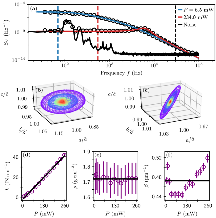
Figure 2: (a) Voltage PSD for 6.5 mW (blue) and 234.0 mW (red) of trapping laser power. Experimental data is depicted with open circles and consists of 40 independent PSD averages and further bin-averaged on a logarithmic horizontal scale for visualization purposes. The solid lines are the maximum-likelihood best fit to eq. (3). The vertical dashed lines mark the bounds on the data used in the fit. The lower bound is color coded with the fitting line and the upper bound (black dashed line) is shared. The noise spectrum (solid black) was collected under identical detection conditions as the other two curves but with no microsphere present. We see a technical noise floor at high frequencies and electronic/laser noise, including 60 Hz harmonics and $1/f$ noise, at low frequencies. The noise peak at around 120 Hz must be omitted when fitting the 234.0 mW spectrum, as indicated by the lower bound (red dashed line). (b) For 6.5 mW of laser power, we plot the isosurfaces of $\mathcal{P}=\exp(-\mathcal{L})$ (see eq. (6)) as a function of fitting parameters $\bm{\theta}$. The isosurfaces are taken at Gaussian widths of 3-sigma (purple), 2-sigma (blue), and a core from the peak (red) to the 1-sigma-width (green). (c) As in (b) but for 234.0 mW of trapping laser power. By fitting the the likelihood data clouds shown in (b) and (c) to a three-variate Gaussian distribution, we extract the best fit parameters $\hat{\bm{\theta}}$ and the variance-covariance matrix $\bm{\Sigma}_{\bm{\theta}}$. (d) Trap strength $k$, (e) microsphere mass density $\rho$, and (f) calibration constant $\beta$, each extracted from PSD fits as a function of laser power $P$. In (d-f), error bars reflect systematic uncertainty calculated by error propagation including correlation among fitted parameters.

To measure the parameter fitting uncertainty and correlation, and inspired by the profile likelihood method [48, 46], we scan $\bm{\theta}$ in the vicinity of $\hat{\bm{\theta}}$ over a volume of parameter space to build up a three-variate probability distribution $\mathcal{P}$ (See Fig. 2(b)-(c)) which is fit to a three-variate Gaussian distribution

$${\mathcal{P}}_{\mathrm{G}}(\bm{\theta};\hat{\bm{\theta}},\bm{\Sigma}_{\bm{\theta}})=\exp\left[-\frac{1}{2}{(\bm{\theta}-\hat{\bm{\theta}})}^{\mathrm{T}}\bm{\Sigma}_{\bm{\theta}}^{-1}(\bm{\theta}-\hat{\bm{\theta}})\right].$$ (7)

The absolute residuals $\lvert\mathcal{P}-{\mathcal{P}}_{\mathrm{G}}\rvert$ are bound below the 1% level. The ${95}^{\mathrm{th}}$ percentile is bound below the 0.1% level (see Appendix D). The vector $\hat{\bm{\theta}}$ resulting from the fit is taken as the best-fit parameter set. The matrix $\bm{\Sigma}_{\bm{\theta}}$ resulting from the fit provides the variance-covariance matrix of the fitted parameters:

$$\bm{\Sigma}_{\bm{\theta}}=\begin{pmatrix}\sigma^{2}_{a}&\sigma^{2}_{ab}&\sigma^{2}_{ac}\\ \sigma^{2}_{ab}&\sigma^{2}_{b}&\sigma^{2}_{bc}\\ \sigma^{2}_{ac}&\sigma^{2}_{bc}&\sigma^{2}_{c}\\ \end{pmatrix}.$$

The uncertainty in parameter $i$ is $\sigma_{i}=\left([\Sigma_{\bm{\theta}}]_{i,i}\right)^{1/2}$ and the correlation coefficient between parameters $i$ and $j$ is $r_{i,j}=[\Sigma_{\bm{\theta}}]_{i,j}/(\sigma_{i}\sigma_{j})$, for $i,j=a,b,c$ (see Appendix D) for a visualization)

The fitting parameters $\bm{\theta}$ may be used to deduce a more physical set of parameters: trap strength $k$, microsphere density $\rho$, and calibration constant $\beta$. Each of the physical parameters $\bm{\Theta}={(k,\rho,\beta)}^{\mathrm{T}}$ are a function of the fitting parameters and constant parameters $R$, $T$, and $\eta$. That is, $\bm{\Theta}=\bm{\Theta}(\bm{\phi})$, where we have defined the vector of independent variables $\bm{\phi}={(\bm{\theta},R,\eta,T)}^{\mathrm{T}}$ (explicit formulae in Appendix A). We now turn to the uncertainty analysis of the constant parameters.

The microsphere radius is known to be $R=1.51~{}$\mathrm{\SIUnitSymbolMicro}\mathrm{m}$$ up to 3.0% uncertainty based on statistical analysis of $\sim 200$ microspheres imaged with a scanning electron microscope [50]. Similar image analysis suggests $\epsilon=a/b-1$ to be 0.027, where $a/b\geq 1$ is the aspect ratio of the imaged microspheres. To first order in $\epsilon$, we estimate corrections to the Stokes friction coefficient due to aspherical geometry [51] to be less than 1%. Similar estimations apply to the microsphere volume, so uncertainty in the radius dominates uncertainty in the geometry. The air temperature, measured with a thermocouple before each trial, was found to vary less than 0.05% over the entire experimental run. The viscosity of air, calculated as a function of temperature with Sutherland’s model, is found to vary over a similarly small range [52]. Sutherland’s model is known to interpolate experimental viscosity data near room temperature with an uncertainty below 0.09% including effects of up to 10% humidity [53]. Since the experiment is performed at atmospheric pressure, the particle-environment interaction is outside the Knudsen regime [54]. As a result, no laser-induced heating of the microsphere is expected, and so thermal equilibrium is assumed.

In light of these observations, the variance-covariance matrix of fitting and constant parameters may be approximated in the block-diagonal form $\mathrm{diag}(\Sigma_{\theta},\sigma^{2}_{R},0,0)$ where the last two zeros reflect the small relative uncertainty in $T$ and $\eta$ compared to that in $a$, $b$, $c$, and $R$. The block diagonal form assumes correlation exists only between the fitted parameters.

We calculate the variance-covariance matrix of the physical parameters in terms of the fitting and constant parameters via the error propagation equation [55] $\bm{\Sigma}_{\bm{\Theta}}=\bm{J}_{\bm{\Theta}}\bm{\Sigma}_{\bm{\phi}}\bm{J}_{\bm{\Theta}}^{\rm T}$. The Jacobian matrix (evaluated at the optimal fitting parameters) is $(J_{\bm{\Theta}})_{i,j}=[\partial\Theta_{i}/\partial\phi_{j}]_{\bm{\theta}=\hat{\bm{\theta}}}$. We have verified that the parameters and uncertainties deduced by the procedure described here and conveniently visualized in Fig. 2(b)-(c) agree quantitatively with the Monte-Carlo method which generates and fits many artificial PSDs by sampling the appropriate gamma distribution. Our technique yields directly the probability density, sidestepping the need for binning and fitting or kernal-density estimating the Monte-Carlo results.

We now understand how to estimate $k$, $\rho$, and $\beta$, including uncertainty and correlation, from an experimental voltage PSD $\hat{S}_{V}$. The results are presented in Fig. 2(d)-(f) for experiments on the same trapped microsphere and which scan the trapping laser power from 6.5 to 257.2 mW. We observe no unexpected dependence of the physical parameters on laser power except for the calibration constant which exhibits a non-monotonic curve, first decreasing then increasing with laser power (Fig. 2(d)). Thus, we conclude heating of the microsphere due to the laser is inconsequential because of the strong environmental coupling. This is not the case for experiments in vacuum [54]. The trend in $\beta$ is reproducible when the experiment is repeated with different microspheres, suggesting the source is most likely slight beam deviations caused by the half wave plate/polarizing beamsplitter pairs used to control the trapping and detected power.

III Mass measurement technique

Upon learning PSD fitting parameters, presented in section II, it is straightforward to estimate the mass using the density and radius of the microsphere. However, the equipartition theorem, ${k}_{\mathrm{B}}T=m\langle\dot{x}^{2}\rangle=k\langle x^{2}\rangle$, provides two additional possibilities. The three mass measurements written in terms of the augmented independent variables $\bm{\phi}^{\prime}={(a,b,c,\langle\dot{V}^{2}\rangle,\langle V^{2}\rangle,R,\eta,T)}^{\mathrm{T}}$ read

$$m_{1}(\bm{\phi}^{\prime})=\frac{4}{3}\pi R^{3}\rho\,,$$ (8)

$$m_{2}(\bm{\phi}^{\prime})=\frac{{k}_{\mathrm{B}}T}{\langle\dot{V}^{2}\rangle}\beta^{2}\,,$$ (9)

$$m_{3}(\bm{\phi}^{\prime})=\frac{\langle V^{2}\rangle}{\langle\dot{V}^{2}\rangle}k\,.$$ (10)

The benefit of $m_{2}$ and $m_{3}$ is that, once a PSD fit is used to calibrate the system, further data can be collected to estimate the variances $\langle\dot{V}^{2}\rangle$ and $\langle V^{2}\rangle$, which may be used to update the mass measurement in the case it changes with time. Of course, there is nothing to update if the mass is unchanging. Nonetheless, to make use of methods $m_{2}$ or $m_{3}$, we must make an adequate estimate of the required variances. In Fig. 3(a)-(b) we show the histograms of position and velocity (proportional to $V$ and $\dot{V}$, respectively) for high and low trapping laser power. The histograms consists of data from a single 0.3 second trial. Overlaid on each histogram are Gaussian fits with variance as the only free parameter. Uncertainty in the variance calculation is taken as the standard deviation of variances calculated across ten trials.

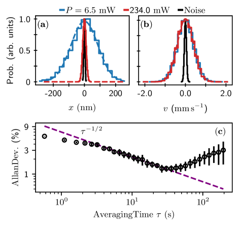
Figure 3: (a) Position probability density (solid steps) of the microsphere’s position over a single 0.3 second trial for 6.5 mW (blue) and 234.0 mW (red) of trapping laser power. Dashed lines correspond to a Gaussian fit with variance as the only free parameter. The black line is a histogram of the signal when no microsphere is present. (b) Velocity probability density. Colors are shared with (a). As expected by the equipartition theorem, the width of the position probability density gets narrower with increasing laser power while the width velocity probability density remains constant. All curves in (a) and (b) are normalized by their maximum value. (c) The relative Allan deviation of variance calculated from a 14 minute voltage signal decreases with increasing averaging time according to a $-1/2$ power law. The decay trend continues until a minimum of about 1% is reached in 30 seconds. Normalization is provided by the value of variance corresponding to the minimum Allan deviation. Error bars reflect the standard deviation of three trials.

For an uncorrelated voltage trace of length $\tau$, the uncertainty in the variance estimate scales as $\tau^{-1/2}$, which is a thermally-limited trend. However, at short times ($\tau<m/\gamma$), the data is correlated due to the microsphere’s dynamics and, at long times, slow drifts in the system tend to affect the signal’s variance. One way to quantify those correlations and to determine the optimal time over which our measurements are thermally limited is performing an Allan-deviation stability analysis [56, 57, 22, 28]. Figure 3(c) shows the results of our Allan-deviation experiment performed with 22.8 mW of trapping laser power. Accordingly, our system is stable out to about 30 s, so using 0.3 s of data for estimating the variances allows for 100 independent mass measurements before the slow drifts demand recalibration of the apparatus. It is in this sense that methods $m_{2}$ and $m_{3}$ are faster than $m_{1}$.

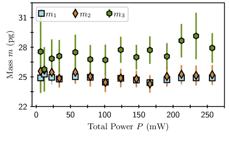
Figure 4: Mass measurement comparison: blue squares, orange diamonds, and green hexagons denote, respectively, $m_{1}$, $m_{2}$, and $m_{3}$. mass measurements as the total trapping power $P$ is varied. Error bars denote the systematic uncertainties ${\sigma}^{\mathrm{sys.}}_{m_{i}}$, $i=1,2,3$. Statistical uncertainties ${\sigma}^{\mathrm{stat.}}_{m_{i}}$ are calculated as standard deviations across the ensemble of mass estimates at different laser powers.

In Fig. 4 we show the results of our three mass measurement procedures. We find $\bar{m}_{1}=24.8~{}$\mathrm{p}\mathrm{g}$$, $\bar{m}_{2}=25.1~{}$\mathrm{p}\mathrm{g}$$, and $\bar{m}_{3}=27.4~{}$\mathrm{p}\mathrm{g}$$ where the over bar denotes an average over the 14 experiments at different total trapping laser powers. Error bars reported are calculated by considering covariance of the PSD fitting parameters, and uncertainties in both fixed parameters and variances. We consider such error bars systematic uncertainty, denoted ${\sigma}^{\mathrm{sys.}}_{m_{i}}$, $i=1,2,3$. The statistical uncertainty (or fluctuation), denoted ${\sigma}^{\mathrm{stat.}}_{m_{i}}$, is calculated as standard deviation across the 14 experiments at different laser powers. Measurement $m_{1}$, which is based entirely on the PSD analysis, has the smallest relative error bars (${\bar{\sigma}}^{\mathrm{sys.}}_{m_{1}}/\bar{m}_{1}=3.0\%$) and the smallest relative statistical uncertainty (${\sigma}^{\mathrm{stat.}}_{m_{1}}/\bar{m}_{1}=0.9\%$). Measurement $m_{2}$, which supplements the PSD analysis by estimating the voltage-derivative variance, agrees well with $m_{1}$, albeit with relative error bars at 4.1% and relative statistical fluctuations at 1.6%. The benefit of $m_{2}$ is that, once an initial PSD analysis is performed, parameters like mass (or temperature) can be subsequently updated 10 times faster than collecting data for additional PSD analysis. Measurement $m_{3}$ has the largest systematic and statistical relative uncertainties, 6.7% and 3.0% respectively. Furthermore, method $m_{3}$ displays additional systematic error because it deviates from $m_{1}$ and $m_{2}$ by nearly 10%. We speculate on the source of this uncertainty in the next section.

For comparison, the mass according to the manufacturer values of density ${\rho}_{\mathrm{Bangs}}=2.0~{}$\mathrm{g}~{}\mathrm{c}\mathrm{m}^{-3}$$ ($\sigma_{{\rho}_{\mathrm{Bangs}}}/{\rho}_{\mathrm{Bangs}}=20\%$) and our radius measurement $R=1.51~{}$\mathrm{\SIUnitSymbolMicro}\mathrm{m}$$, $(\sigma_{R}/R=2.9\%)$ is ${m}_{\mathrm{Bangs}}=28.84~{}$\mathrm{p}\mathrm{g}$$ with an uncertainty of 22% which agrees within the uncertainty tolerance of all our mass measurements, despite the discrepancy of the mean values.

IV Discussion

The systematic bias in $m_{3}$ of Fig. 4 is hypothesized to be dominated by the low frequency electronic noise apparent in Fig. 2(a). By selecting an appropriate lower bound for the fit, the spectral method easily removes the influence of the noise resonances, the most severe of which appears at 120 Hz with a width of about 100 Hz. However, the time domain estimate of $\langle V^{2}\rangle$ includes variance due to that noise. To estimate the effects of such noise, we can model the experimental PSD as the sum of the best fit PSD and the experimental noise PSD containing the noise peak near 120 Hz, $S_{V}(f)={S}^{\mathrm{best}}_{V}(f)+{S}^{\mathrm{noise}}_{V}(f)$. Using Parseval’s theorem, $\langle q^{2}\rangle=\int_{0}^{\infty}S_{q}(f)\mathrm{d}f$, we have

$$\langle V^{2}\rangle\approx{\langle V^{2}\rangle}_{\mathrm{PSD}}+\int_{70~{}$\mathrm{H}\mathrm{z}$}^{170~{}$\mathrm{H}\mathrm{z}$}{S}^{\mathrm{noise}}_{V}(f)\mathrm{d}f\,,$$ (11)

where $\langle V^{2}\rangle$ is the variance of the voltage signal observed in the time domain, ${\langle V^{2}\rangle}_{\mathrm{PSD}}={k}_{\mathrm{B}}T\beta^{2}/k$ is the variance estimate provided by the PSD parameters. The excess variance $\Delta\langle V^{2}\rangle\equiv\lvert\langle V^{2}\rangle-{\langle V^{2}\rangle}_{\mathrm{PSD}}\rvert$ is about 10% of ${\langle V^{2}\rangle}_{\mathrm{PSD}}$ , which agrees with the discrepancy between $m_{3}$ and and the other measurements. The quantity $\Delta\langle V^{2}\rangle$ can also be estimated by numerically integrating the observed noise spectrum. We find that the integral of the noise PSD in frequency band from 70 Hz to 170 Hz predicts the observed excess variance and hence also the bias in $m_{3}$.

The effects of low frequency noise resonances are suppressed when estimating $\langle\dot{V}^{2}\rangle$. The reason is because, in general, $S_{\dot{q}}\left(f\right)=(2\pi f)^{2}S_{q}(f)$, so high frequency components of a signal have a quadratically larger weighting factor in the variance compared to low frequency noise. We find, by direct calculation on our data, $\Delta\langle\dot{V}^{2}\rangle\sim 2\%$, which agrees with numeric integration of ${S}^{\mathrm{noise}}_{\dot{V}}(f)$ over all frequencies above 80 kHz.

A recent experimental effort [23] measured the mass of $0.143~{}$\mathrm{\SIUnitSymbolMicro}\mathrm{m}$$ radius $\mathrm{SiO_{2}}$ spheres optically trapped in vacuum to be 4.01 fg with 2.8% uncertainty with 40 s of position data. Their oscillating electric field method makes no assumption on particle shape or density, though a density of $2.2~{}$\mathrm{g}~{}\mathrm{c}\mathrm{m}^{-3}$$ agrees with their measurements. In [34], a $2.6~{}$\mathrm{\SIUnitSymbolMicro}\mathrm{m}$$ radius sphere is optically trapped and levitated with a static electric field as the trapping laser power is reduced, resulting in a mass measurement of 84 pg with 1.8% uncertainty with 42 minutes of data. The density is also measured to be 1.55 $\mathrm{g}~{}\mathrm{c}\mathrm{m}^{-3}$ with 5.16% uncertainty. A third strategy used in [24] stabilizes oscillations of a $0.082~{}$\mathrm{\SIUnitSymbolMicro}\mathrm{m}$$ radius sphere in the nonlinear-trapping regime to deduce the detector calibration constant with 1.0% uncertainty and a mass of 3.63 fg with 2.2% uncertainty. Finally, very recent work [35] used a drop-recapture method and camera-based detection with time resolution that could not quite resolve the microsphere’s instantaneous velocity. Fitting position autocorrelation functions, they measure their resin particle’s radius to be 2.3 $\mathrm{\SIUnitSymbolMicro}\mathrm{m}$ with 4.3% statistical uncertainty. In the drop-recapture experiments, 90 s worth of trials are used to deduce a mass of 55.8 pg with 1.4% statistical uncertainty and 13% systematic uncertainty. The authors combine the radius and mass measurements to deduce a density of 1.1 $\mathrm{g}~{}\mathrm{c}\mathrm{m}^{-3}$ with 9.1% statistical uncertainty.

As a comparison, we present a summary of our physical parameter values and uncertainties in Table 1. Based entirely on thermal equilibrium analysis, our two most accurate mass estimates have uncertainties of 3% to 4% as compared to the 1% to 2% uncertainty in vacuum-dependent and 13% in the air-based, nonequilibrium methods. Further, all of our measurements are made with significantly less position data. Interestingly, our density measurement has comparable accuracy to the recent body of work using $\mathrm{SiO_{2}}$ particles, all of which sourced particles from the same manufacturer. The variability and apparent radius dependence of measured density values underscores the parameter’s uncertainty inherint to the manufacturing process.

Most of the existing mass measurement methods are demonstrated in a high vacuum environment where the experimental goals often center around ground-state cooling or exceptionally sensitive force transduction. Additionally, the existing methods rely on forces external to the trap, often driving the system out of equilibrium and limiting their utility as environmental sensors. Our method has the advantages of speed in that between $10\times$ and $100\times$ less data is required compared to other methods; environmental coupling, which unlocks future sensing applications; and simplicity in that no additional experimental set up is required beyond trapping and monitoring.

Disadvantages include the requirements of environmental coupling, enough spatiotemporal resolution to resolve the instantaneous velocity, and accurate knowledge of the particle radius. While an advantage for future applications, environmental coupling critically limits heating effects of the trapping laser and enables fast equilibration with the environment, so our method will face complications in vacuum-based experiments. Accurate heating/damping models and longer data traces could possibly overcome such concerns. Instantaneous velocity resolution enables our fastest measurement, $m_{2}$, but can be much more difficult in a liquid environment, though certainly possible [38]. Accurate knowledge of the trapped particle geometry was quantified statistically in our experiment, but less uniform samples could significantly alter the error analysis. In these cases, in situ measurements of the trapped particle with optical microscopy, light scattering, or autocorrelation function analysis could improve the error budget.

Table 1: Table of values and uncertainties. Reported values are the average over the power scan experiment, except for $k$ and $\langle V^{2}\rangle$ for which we report the range since these quantities scale linearly with $P$. Also reported are the relative systematic uncertainties (sys.) averaged over the power scan experiment and the statistical uncertainties (stat.) which express the relative standard deviation over the power scan, where applicable.

Quantity	Value	Uncertainty (%)		Unit
		sys.	stat.
$R$	1.51	$2.9$	-	$\mathrm{\SIUnitSymbolMicro}\mathrm{m}$
$\eta$	18.295	$0.04$	-	$\mathrm{\SIUnitSymbolMicro}\mathrm{P}\mathrm{a}~{}\mathrm{s}$
$T$	295.50	$0.05$	-	$\mathrm{K}$
$\langle\dot{V}^{2}\rangle\times 10^{3}$	36.4	$2.4$	-	$\mathrm{\SIUnitSymbolMicro}\mathrm{s}^{-1}$
$\langle V^{2}\rangle\times 10^{3}$	(0.03, 1.53)	$8.9$	-	arb. units
$k$	(0.66, 49.1)	$3.1$	-	$\mathrm{f}\mathrm{N}~{}\mathrm{n}\mathrm{m}^{-1}$
$\rho$	1.72	$5.9$	$0.9$	$\mathrm{g}~{}\mathrm{c}\mathrm{m}^{-3}$
$\beta$	0.47	$1.6$	$5.0$	$\mathrm{\SIUnitSymbolMicro}\mathrm{m}^{-1}$
$m_{1}$	24.8	$3.0$	$0.9$	$\mathrm{p}\mathrm{g}$
$m_{2}$	25.1	$4.1$	$1.6$	$\mathrm{p}\mathrm{g}$
$m_{3}$	27.4	$6.7$	$3.0$	$\mathrm{p}\mathrm{g}$

V Conclusions

We have explored spectral and equipartition methods by which to measure an optically trapped microsphere’s mass while in thermal equilibrium with air. With the former, we accurately extract physical parameters of trap strength $k$, microsphere density $\rho$, and detector calibration constant $\beta$ with 3 seconds of data. The initial spectral calibration step also yields the mass $m_{1}$ with 3.0% uncertainty. The subsequent equipartition method $m_{2}$ achieves an uncertainty of 4.1% in 0.3 seconds.

The work presented here demonstrates the sensitivity of optical tweezers in a scenario of strong environmental coupling, suggesting applications in air-based sensing. For example, single-site ice nucleation could be monitored in real time as a change in mass of the trapped particle. Alternatively, in a system of constant mass, one could first measure the mass using the spectral method and then use the equipartition method to measure changes in temperature within the trapping medium, which could be driven out of equilibrium with a temperature gradient to probe temperature-gradient-induced turbulence at small scales of space and time.

The equipartition theorem may be challenged by non-equilibrium dynamics. However, in the hydrodynamic regime where thermodynamic state variables are relevant in the sense of quasi-equilibrium, we believe our method will be quite applicable. The small sensor size means the dynamics are fast to respond to changes in the environment (on the scale of $m/\gamma\sim 45~{}$\mathrm{\SIUnitSymbolMicro}\mathrm{s}$$ in this work). Even in the complete absence of thermal equilibrium, where the notion of temperature is no longer defined, our position and velocity data may be used to compute more general velocity structure functions when the simple variance appearing in the equipartition theorem is insufficient [58, 59]. We consider such non-equilibrium studies a fruitful direction for future optical tweezer experiments.

VI Acknowledgments

The authors are grateful to Y. Stratis, I. Bucay, Y. Lu, K. S. Melin, S. Bustabad, L. Gradl for helping with daily lab activities and making the lab a pleasant environment. We also specially thank A. Helal for assisting with SEM imaging of the silica microspheres.

Appendix A Parameter conversions

The physical parameters, denoted by the column vector $\bm{\Theta}={(k,\rho,\beta)}^{\mathrm{T}}$, are functions of the independent variables $\bm{\phi}={(a,b,c,R,\eta,T)}^{\mathrm{T}}$. First we define

$$d_{1}\equiv b+\sqrt{ac}\,,$$ (12)

$$d_{2}\equiv b+2\sqrt{ac}\,.$$ (13)

Then, for $\bm{\Theta}(\bm{\phi})$, we have

$$k(\bm{\phi})=12\pi^{2}\eta R\sqrt{\frac{a}{d_{2}}}\,,$$ (14)

$$\rho(\bm{\phi})=\frac{9\eta}{4\pi R^{2}}\sqrt{\frac{c}{d_{2}}}\,,$$ (15)

$$\beta^{2}(\bm{\phi})=\frac{6\pi^{3}\eta R}{{k}_{\mathrm{B}}Td_{2}}\,.$$ (16)

The mass measurements $\bm{m}={(m_{1},m_{2},m_{3})}^{\mathrm{T}}$ are a function of the augmented independent variables, $\bm{\phi}^{\prime}=(a,b,c,\langle\dot{V}^{2}\rangle,\langle V^{2}\rangle,R,\eta)$ (noting that $\partial\bm{m}/\partial T=0$). For explicit formulae, we have

$$m_{1}(\bm{\phi}^{\prime})=3\eta R\sqrt{\frac{c}{d_{2}}}\,,$$ (17)

$$m_{2}(\bm{\phi}^{\prime})=\frac{6\pi^{3}\eta R}{d_{2}}\frac{1}{\langle\dot{V}^{2}\rangle}\,,$$ (18)

$$m_{3}(\bm{\phi}^{\prime})=12\pi^{2}\eta R\sqrt{\frac{a}{d_{2}}}\frac{\langle V^{2}\rangle}{\langle\dot{V}^{2}\rangle}\,.$$ (19)

We next define

$$u_{1}\equiv\frac{3}{16\pi^{3}R^{3}}\,,\hskip 14.22636ptu_{2}\equiv\frac{1}{2\sqrt{6\pi\eta R{k}_{\mathrm{B}}T}}\,,$$ (20)

$$v_{1}\equiv\frac{1}{4\pi^{2}}\,,\hskip 14.22636ptv_{2}\equiv\frac{\pi}{\langle\dot{V^{2}}\rangle}\,,\hskip 14.22636ptv_{3}\equiv\frac{\langle V^{2}\rangle}{\langle\dot{V}^{2}\rangle}\,,$$ (21)

to write the Jacobians

$$\frac{\partial\bm{\Theta}}{\partial\bm{\phi}}=\frac{6\pi^{2}\eta R}{\sqrt{ad_{2}^{3}}}\begin{pmatrix}d_{1}&-a&-\sqrt{a^{3}/c}&2ad_{2}/R&2ad_{2}/\eta&0\\ -u_{1}c&-u_{1}\sqrt{ac}&u_{1}d_{1}\sqrt{a/c}&-4u_{1}d_{2}\sqrt{ac}/R&2u_{1}d_{2}\sqrt{ac}/\eta&0\\ -u_{2}\sqrt{c}&-u_{2}\sqrt{a}&-u_{2}a/\sqrt{c}&u_{2}d_{2}\sqrt{a}/R&u_{2}d_{2}\sqrt{a}/\eta&-u_{2}d_{2}\sqrt{a}/T\end{pmatrix}\,,$$ (22)

$$\frac{\partial\bm{m}}{\partial\bm{\phi}^{\prime}}=\frac{6\pi^{2}\eta R}{\sqrt{ad_{2}^{3}}}\begin{pmatrix}-v_{1}c&-v_{1}\sqrt{ac}&v_{1}d_{1}\sqrt{a/c}&0&0&2v_{1}d_{2}\sqrt{ac}/R&2v_{1}d_{2}\sqrt{ac}/\eta\\ -v_{2}\sqrt{c/d_{2}}&-v_{2}\sqrt{a/d_{2}}&-v_{2}a/\sqrt{cd_{2}}&-v_{2}\sqrt{ad_{2}}/\langle\dot{V}^{2}\rangle&0&v_{2}\sqrt{ad_{2}}/R&v_{2}\sqrt{ad_{2}}/\eta\\ v_{3}d_{1}&-v_{3}a&-v_{3}\sqrt{a^{3}/c}&-2v_{3}ad_{2}/\langle\dot{V}^{2}\rangle&2v_{3}ad_{2}/\langle V^{2}\rangle&2v_{3}ad_{2}/R&2v_{3}ad_{2}/\eta\end{pmatrix}\,,$$ (23)

which are needed for error propagation.

Appendix B Experimental Set Up

Our experiment is sketched in Fig. 1 of the main text and consists of a 1064 nm laser (Innolight Mephisto Laser System) which is split into two counter-propagating, cross-linearly-polarized, $\mathrm{TEM}_{00}$ beams. Each beam is passed through a 3 mm focal-length aspheric lens (Thorlabs C330TMD-C) with foci offset by about $25~{}$\mathrm{\SIUnitSymbolMicro}\mathrm{m}$$ along the optical axis. One beam is maintained at a higher power and provides the confining potential at its focus while the counter-propagating beam cancels the scattering force from the forward beam which otherwise ejects the microsphere from the trap. The two counter-propagating beams thus form a dual beam optical trap [1, 37]. An acoustic-optical modulator (AOM) (IntraAction Corp, ATM-801A6 modulator) shifts the frequency of the counter-propagating beam by 80 MHz which, in conjunction with the cross polarization of the two beams, eliminates interference effects on the trapping potential. Additionally, the AOM gives fine control over the power imbalance of the two trapping beams. Silica microspheres (Bangs Laboratories, Inc, catalog number SSD5001, nominal radius $1.5~{}$\mathrm{\SIUnitSymbolMicro}\mathrm{m}$$) are spread across a glass coverslip which is fixed above the center of the trap and may be agitated with a homemade piezoelectric transducer to release microspheres on demand.

The forward beam is isolated with a second polarizing beamsplitter and its wave front is split with a D-shaped cut mirror (Thorlabs, model BBD05-E03). Each half of the split beam is directed into the two ports of a balanced photo detector (Thorlabs, model PDB120C, bandwidth DC-75 MHz), which provides a voltage proportional to the optical power imbalance in the two halves of the beam. The voltage signal is digitized (GaGe Razor 1622 Express CompuScope) and saved to disk for analysis. When a microsphere is trapped, the surrounding air causes it to undergo Brownian motion. As the microsphere deviates from the center of the trap, it scatters and deflects the trapping light and the resulting signal from the balanced detector is proportional to the displacement of the microsphere along the transverse direction perpendicular to the cut of the mirror. The forward beam’s propagation direction is taken as the $z$-axis and its polarization as the $y$-axis. The cut mirror’s edge is aligned to the $y$ axis and measures the displacement of the particle along the $x$-axis. The entire setup is enclosed in a homemade multi-chamber acrylic box [15, 11] to mitigate effects of air currents. A thermocouple placed near the trap monitors the temperature of the air. Laser power is controlled with half wave plate and polarizing beamsplitter pairs, one near the laser head to control the total trapping power $P$, and one before the cut mirror maintains the total detected power at $\sim 35~{}$\mathrm{\SIUnitSymbolMicro}\mathrm{W}$$.

Appendix C Methods

Here we detail the methods of our data analysis.

C.1 Raw data

The balanced photodetector has two ports, $a$ and $b$, for measuring optical power. The device provides three continuous voltage signals, ${V}_{\mathrm{a}}(t)$, ${V}_{\mathrm{b}}(t)$, and $V_{-}(t)={V}_{\mathrm{b}}(t)-{V}_{\mathrm{a}}(t)$ with a bandwidth of 0 to 75 MHz. Once a microsphere is trapped and just before an experimental trial begins, we make a measurement of $V_{+}(0)={V}_{\mathrm{a}}(0)+{V}_{\mathrm{b}}(0)$. We then make a digitized record of $V_{-}(t)$ consisting of $N=2^{24}\approx 1.7\times 10^{7}$ samples at a rate of $r=5\times 10^{7}$ Hz. Hence, one trial is of length $\mathcal{T}=N/r=0.336$ s. We collect 10 trials for a total of 3.36 s of data at each of 14 different trapping laser powers. Note that while $V(t)$ is adimensional, we refer to it as the voltage signal. Similarly $\dot{V}(t)$ is referred to as voltage-derivative signal.

C.2 Bin-averaging

Post processing begins by, for each trial, forming a data set $V=\{V_{j}\}$, where $V_{j}=V_{-}(t_{j})/V_{+}(0)$ is the signal at time $t_{j}=j/r$, for $j=0,1,\dots,N-1$. Next, we average $V_{j}$ over non-overlapping bins of size $M=2^{8}$ to form $\langle V\rangle(M_{j})$, where $M_{j}$ is the ${j}^{\mathrm{th}}$ time bin and $j=0,1,\dots,\left(N/M\right)-1$. The bin-averaging procedure reduces uncorrelated voltage noise by a factor of $M^{-1/2}$, and decreases the sampling rate and number of points both by a factor of $M^{-1}$. Explicitly, the ${j}^{\mathrm{th}}$ $M$-bin average of a digitized quantity $q$ is

$$\langle q\rangle(M_{j})=\frac{1}{M}\sum_{i=0}^{M-1}q_{jM+i}\,,$$ (24)

where $q_{jM+i}$ is the ${(jM+i)}^{\mathrm{th}}$ element of $q$. For our choice of $M=2^{8}$, the number of data points becomes $N/M=2^{16}\approx 6.6\times 10^{4}$. The new effective sampling rate, $r/M=195~{}$\mathrm{k}\mathrm{H}\mathrm{z}$$, is still roughly 10 times faster than the momentum decay rate $\gamma/m\approx 22~{}$\mathrm{k}\mathrm{H}\mathrm{z}$$ which sets the time scale of correlated ballistic motion. Since a 256-bin average is always the first step in our data processing, we reuse the notation $V=\{V_{j}\}$ to denote a trial after processing with Eq. (24). Additionally, we take $N$ and $r$ to henceforth denote the values after bin averaging. The instantaneous velocity may now be meaningfully computed.

C.3 Instantaneous velocity

The instantaneous velocity of the microsphere is proportional to the voltage-derivative signal. We approximate the derivative numerically with the $8^{\mathrm{th}}$-order central finite difference approximation

$$\begin{split}\dot{V}_{j}=r\bigg{(}&\frac{V_{j-4}}{280}-\frac{4V_{j-3}}{105}+\frac{V_{j-2}}{5}-\frac{4V_{j-1}}{5}+\\ &\frac{4V_{j+1}}{5}-\frac{V_{j+2}}{5}+\frac{4V_{j+3}}{105}-\frac{V_{j+4}}{280}\bigg{)}+\mathcal{O}(r^{-8})\,.\end{split}$$ (25)

With this approximation, we can compute a total of $N-8$ velocities corresponding to the times $t_{j}^{(\dot{V})}=t_{j}$ for $j=4,5,\dots,N-5$.

C.4 Signal variance

The voltage signal variance $\langle V^{2}\rangle$ and voltage-derivative signal variance $\langle\dot{V}^{2}\rangle$ are needed for mass measurement methods $m_{2}$ and $m_{3}$. For the quantities $q=V,\dot{V}$, we fit the density histogram of $\{q_{j}\}$ to a normalized one-dimensional Gaussian distribution

$${\mathcal{P}}_{\mathrm{G_{1}}}(q;\langle q^{2}\rangle)=\frac{1}{\sqrt{2\pi\langle q^{2}\rangle}}\exp\left(\frac{-q^{2}}{2\langle q^{2}\rangle}\right)\,,$$ (26)

for the free parameter $\langle q^{2}\rangle$. The fits are performed as un-weighted chi-squared minimizations. We take $L=10$ trials of each data set. The statistical variance of $\langle q^{2}\rangle_{i}$ across trials $i=0,1,\dots L-1$ relative to the mean value $\mu_{\langle q^{2}\rangle}=\frac{1}{L}\sum_{i}\langle q^{2}\rangle_{i}$ is

$$\sigma^{2}_{\langle q^{2}\rangle}=\frac{1}{L}\sum_{i=0}^{L-1}\left(\langle q^{2}\rangle_{i}-\mu_{\langle q^{2}\rangle}\right)^{2}\,.$$ (27)

The square-root of equation (27) gives the uncertainty in $\langle q^{2}\rangle$ for the purposes of error propagation.

Both $\langle\dot{V}^{2}\rangle$ and $\langle V^{2}\rangle$ are sensitive to the amount of initial bin averaging. The choice of $M=256$ was arrived at by converging the two variances as a function of $M$. Too little averaging and the voltage-derivative variance is over-estimated. Too much averaging and both variances are under-estimated. $M=256$ is between these two extremes where the change in variance is minimal for a small change in $M$.

The Allan deviation, is the square-root of the Allan variance (two-sample variance) [56],

$$\mathcal{A}^{2}_{\langle q^{2}\rangle}(\tau)=\frac{1}{A-1}\sum_{j=0}^{A-2}\frac{1}{2}\left[\langle q^{2}\rangle(\tau_{j+1})-\langle q^{2}\rangle(\tau_{j})\right]^{2}\,,$$ (28)

where $A=\mathcal{T}/\tau$ is the number of independent length-$\tau$ blocks in a trial of total length $\mathcal{T}$ and $\langle q^{2}\rangle(\tau_{j})$ is the ${j}^{\mathrm{th}}$ bin-average of $q^{2}$ with $M=r\tau$ points.

C.5 Voltage power spectral density: Bartlett’s method

Next, we describe our method of extracting the experimental voltage PSD. The one-sided PSD calculated from a single trial $\{V_{j}\}$ is

$$\hat{S}_{V,k}=\frac{2}{W_{N}}\left\lvert\sum_{j=0}^{N-1}w_{j}^{(N)}V_{j}\exp\left[-2\pi i\frac{jk}{N}\right]\right\rvert^{2}\,,$$ (29)

$$f_{k}=\frac{kr}{N}\,,$$ (30)

for $k=0,1,\dots,N/2$. We have introduced the notation $\hat{S}_{V,k}=\hat{S}_{V}(f_{k})$. Additionally, $w_{j}^{(N)}=w(t_{j};N)$ is a windowing function for a trial of size $N$ and

$$W_{N}=\frac{1}{r}\sum_{j=0}^{N-1}\left\lvert w_{j}^{(N)}\right\rvert^{2}\,,$$ (31)

is a power correction for the windowing procedure. The factor $2/W_{N}$ ensures Parseval’s theorem $\sum_{k}\hat{S}_{V,k}=\langle V^{2}\rangle$. Note that if $w(t_{j};N)=1$, then $W_{N}=\mathcal{T}$. We use the a Hamming window

$$w(t_{j};N)=0.54-0.46\cos\left(\frac{2\pi t_{j}}{t_{N-1}}\right)\,,$$ (32)

for which $W_{N}=0.4194\mathcal{T}$ in the continuum limit $N\rightarrow\infty$ and $r\rightarrow 0$. The choice of window was found to be inconsequential for parameter extraction except for small deviations at the lowest few trapping-laser powers, i.e., the over-damped oscillator regime. This observation appears to be in analogy with [48] where Bartlett’s method is used in conjunction with windowing because of the accuracy it affords parameter extraction at high vacuum pressure, i.e., high damping.

$V_{j}$ is proportional to the microsphere’s position at time $t_{j}$, and the microsphere is subject to a stochastic force $F(t_{j})\propto\xi(t_{j})$, where $\xi(t_{j})$ is a real-valued, Gaussian distributed, white noise random process with zero mean and delta-correlation. A single trial’s PSD $\hat{S}_{V,k}$, then, is subject to fluctuations $\propto\lvert\tilde{\xi}(f_{k})\rvert^{2}$ where $\tilde{\xi}(f_{k})$ is the discrete Fourier transform of the particular instance $\xi(t)$ present in that trial. Since $\xi(t)$ is Gaussian-distributed, $\tilde{\xi}(f_{k})$ is a complex number with real and imaginary parts independent and identically Gaussian distributed. $\lvert\tilde{\xi}(f_{k})\rvert^{2}$ is the sum of two squared Gaussian-distributed variables which is exponentially distributed [49]. Thus, the experimental $\hat{S}_{V,k}$ is an exponentially distributed random process with mean and standard deviation equal to the theoretical PSD, $S_{V,k}$:

$$\mathcal{P}(\hat{S}_{V,k})=\frac{1}{S_{V,k}}e^{-\hat{S}_{V,k}/S_{V,k}}$$ (33)

It is desirable to suppress this intrinsic noise so that fitting experimental data yields precise parameters.

The idea of Bartlett’s method [45] is to average several independent noisy PSDs. First, the time-domain signal is segmented into $n$ independent blocks. Then, for each block we calculate a PSD, and average the results. To proceed, we form $V^{(\ell)}_{j}$ where $\ell=0,1,\dots,n-1$ enumerates blocks of size $N/b$ given by partitioning each of the $L=10$ trials of size $N$ into $b=4$ blocks. Hence, there are a total of $n=Lb=40$ blocks of size $N/b=2^{14}$ (or length 83.9 $\mathrm{m}\mathrm{s}$). Bartlett’s PSD estimate may be written

$$\hat{\bar{S}}_{V,k}=\frac{1}{n}\sum_{\ell=0}^{n-1}\hat{S}_{V^{(\ell)},k}$$ (34)

$$\bar{f}_{k}=\frac{krb}{N}\,,$$ (35)

where it is understood that here the $N$ appearing in Eq. (29) is the size of $V^{(\ell)}$, namely $N/b$.

Due to the PSD averaging, $\hat{\bar{S}}_{V,k}$ is Gamma distributed (the convolution of $n$ exponential distributions) [47]:

$$\mathcal{P}(\hat{\bar{S}}_{V,k})=\frac{1}{S_{V,k}}\frac{n^{n}}{\Gamma(n)}\left(\frac{\hat{\bar{S}}_{V,k}}{S_{V,k}}\right)^{n-1}\exp\left(-n\frac{\hat{\bar{S}}_{V,k}}{S_{V,k}}\right)\,,$$ (36)

where $\Gamma(n)=(n-1)!$ is the gamma function.

The probability of measuring the model $S_{V,k}=S_{V}(f_{k},\bm{\theta})$ given the data $\hat{\bar{S}}_{V}$ is the product over $k$ of Eq. (36), i.e.,

$$\mathcal{P}(\hat{\bar{S}}_{V}|\bm{\theta})=\prod_{k=0}^{N/2-1}\mathcal{P}(\hat{\bar{S}}_{V,k}).$$ (37)

Henceforth and in the main we simplify the notation and take $\hat{S}_{V}(f_{k})$ to denote the Bartlett PSD discussed here. Optimal parameters $\hat{\bm{\theta}}$ are found by maximizing Eq. (37), or minimizing its negative-logarithm $\mathcal{L}(\hat{S}_{V},\theta)$ (Eq. (6) of the main text).

Appendix D Uncertainty analysis

In this section, we elaborate on the quantification of uncertainty in voltage measurements, fitting parameters, and fixed parameters.

D.1 Voltage measurement uncertainty

The signal digitizer has 16 bits and a full-scale input range of 2 $V$ ($\pm 1~{}$\mathrm{V}$$). However, the manufacturer reports an effective-number-of-bits of 11.7 (meaning 4.3 bits are polluted by electronic noise). The resolution of the digitizer is the voltage range allotted to the least significant bit (LSB): $\mathrm{LSB}=2V/2^{11.7}=601~{}$\mathrm{\SIUnitSymbolMicro}\mathrm{V}$$. The systematic uncertainty in the measured voltage $V_{-}$ due to digitization is estimated to be $\sigma_{V_{-}}=\frac{1}{2}\mathrm{LSB}$. In the experiments reported on here, we need to resolve voltage variances. The smallest observed standard deviation is $\langle V^{2}_{-}\rangle^{1/2}=0.02~{}$\mathrm{V}$$, so a worst-case estimate of the systematic uncertainty due to digitization is about 1.5%. Upon bin-averaging with $M=256$ points, the standard deviation of a purely electronic-noise signal is found to be reduced by the expected factor $M^{-1/2}=1/16$ (which we have verified with experimental data). Thus, the systematic uncertainty in voltage measurements due to this electronic noise is $\sigma_{V_{-}}/\langle V^{2}_{-}\rangle^{1/2}=0.09\%$, which is ignorable compared to other uncertainties.

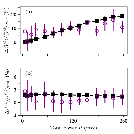
Figure 5: (a) Excess variance is observed in the time domain voltage signal as compared to the variance expected by fitting the PSD (purple circles). The black squares reflect the integral of the noise spectrum over the 120 Hz peak under the same normalization. (b) Excess variance observed in the voltage-derivative signal (purple circles) and the expected excess variance based in the integral of the noise spectrum from 80 kHz and above. In both panels the dashed line is a guide to the eye, and error bars reflect the statistical variation of variance measurements across 10 trials for each of the 14 different trapping laser powers.

The above discussion considers only electronic noise of the detector and digitizer. However, uncertainty in a measured signal variance is much more significantly affected by laser noise, which includes pointing and power fluctuations. Pointing instability is inherent to the laser and also arises due to mechanical and electrical coupling through the the mirrors and control electronics. The significant resonance observed near 120 Hz in the laser-on noise spectrum (Fig. 2(a) of the main text) accounts well for the excess variance observed in the time domain voltage signal as compared to the variance expected based on PSD fitting, which easily excludes the noise peak in the fitting procedure. In Fig. 5(a) we show the observed excess variance $\Delta\langle V^{2}\rangle=\lvert\langle V^{2}\rangle-{\langle V^{2}\rangle}_{\mathrm{PSD}}\rvert$ as well as the value predicted by integrating the noise spectrum in a band from 70 Hz to 170 Hz. On average, the systematic uncertainty in $\langle V^{2}\rangle$ due to this excess variance is at about 10%, which seemingly explains the systematic over estimate of $m_{3}$ (which is proportional to $\langle V^{2}\rangle$) compared to $m_{1}$ and $m_{2}$.

The voltage-derivative signal is insensitive to the presence of the 120 Hz resonance. Instead, the observed excess variance is well accounted for high frequency noise (above 80 kHz). Figure 5(b) shows the observed and expected excess variance in the voltage-derivative for each set of trials. On average, the systematic uncertainty in $\langle\dot{V}^{2}\rangle$ is about 2%.

D.2 Uncertainty in PSD fitting parameters

The PSD fitting parameters $\bm{\theta}={(a,b,c)}^{\mathrm{T}}$ and their associated variance-covariance matrix $\bm{\Sigma}_{\bm{\theta}}$ are found by calculating Eq. (37) in the vicinity of the optimal parameters (main text Fig. 2(b)-(c)) and fitting the result to a three-dimensional Gaussian. For completeness, the relative uncertainties and correlation coefficients of the fitting parameters are plotted in Fig. 6. We find excellent agreement between the three-variate data and fit in Fig. 7(a) which shows the absolute residual of the fit from the data as a function of percentile for high and low trapping laser powers.

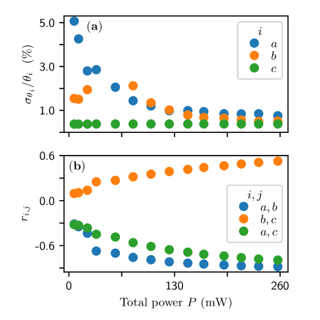
Figure 6: (a) Relative uncertainty in fitting parameters and (b) correlation coefficients at different total trapping laser powers. The parameter $b$ goes through a zero crossing near 65 mW causing the relative uncertainty to diverge. We omit two data points in that region for visualization purposes.

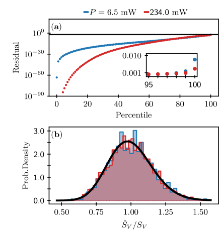
Figure 7: (a) Absolute residual between the fitting-parameter-scan data and three-dimensional Gaussian fit are bounded by 1% (black line). The inset demonstrates the $95^{\mathrm{th}}$ percentile is bound by 0.1%. (b) Distribution of the ratio between PSD data and PSD fit (filled step-plots) and the expected gamma distribution for $n=40$ PSD averages (no free parameters, black line).

The optimal parameters generate a model $S_{V}$ around which the PSD data $\hat{S}_{V}$ is scattered according to the gamma distribution (36). Hence, distribution of $\hat{S}_{V}/S_{V}$ is also gamma-distributed, but with unit mean. In Fig. 7(b) we show the observed distribution of $\hat{S}_{V}/S_{V}$ for high and low trapping laser powers as well as the theoretically expected gamma distribution for $n=40$ PSD averages.

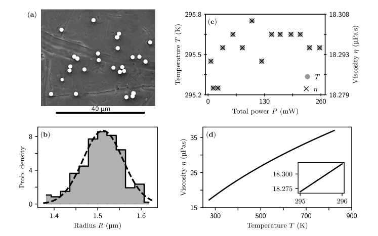
Figure 8: (a) Example SEM image analyzed for the microsphere radius. (b) A density histogram (filled gray step-plot) of the 219 observed radii. The dashed line is a Gaussian fit with mean and variance as free parameters. (c) Observed temperatures (circles) and the corresponding viscosity (crosses) evaluated with the Sutherland model for each set of the 14 sets of trials. (d) Temperature dependence of viscosity according to the Sutherland model (Eq. (38)). The inset shows the linearity of viscosity over the experimentally relevant temperature range.

D.3 Uncertainty in fixed parameters

To fix the microsphere radius, we first took 10 scanning electron microscope (SEM) images of a sample of $3~{}$\mathrm{\SIUnitSymbolMicro}\mathrm{m}$$ diameter microspheres. An example image is shown in Fig. 8(a). We measured the diameter of the imaged spheres using the Particle Sizer plugin [50] for the Fiji distribution of ImageJ, an open source image analysis software. We operated the plugin with default settings and in “single particle mode” to exclude touching and overlapping microspheres. Once an image was analyzed, we manually excluded false positives by inspection. In total, we measured 219 spheres and fit the histogram of measured radii to one-dimensional Gaussian probability density (Fig. 8(b)). The fitting procedure yields a mean of $R=1.512~{}$\mathrm{\SIUnitSymbolMicro}\mathrm{m}$$. The uncertainty of fixing $R$ to this value is taken to be the standard deviation of the fitted distribution, $\sigma_{R}=0.044~{}$\mathrm{\SIUnitSymbolMicro}\mathrm{m}$$. Our measurement provides a marked improvement over the manufacturer-stated radius of 1.5 $\mathrm{\SIUnitSymbolMicro}\mathrm{m}$ with an uncertainty of 10%.

The temperature $T$ is measures at the beginning of each set of trials using type-K thermocouple. Over the entire experiment reported on here, the temperature varied by only 0.05%. As a result, we take $T$ of a set of trials to be given by the value measured at the start of collection and the uncertainty is taken as $\sigma_{T}=0$ in comparison to other uncertainties.

The Dynamic viscosity $\eta$ as a function of temperature $T$ is evaluated with the Sutherland model [52, 53] (plotted in Fig. 8(d))

$$\eta(T)=\eta^{\prime}\left(\frac{T}{T^{\prime}}\right)^{3/2}\frac{T^{\prime}+S}{T+S}\,,$$ (38)

in which $\eta=\eta^{\prime}=18.3245~{}$\mathrm{\SIUnitSymbolMicro}\mathrm{P}\mathrm{a}$$ when $T=T^{\prime}=296.15~{}$\mathrm{K}$$, and $S=110.4~{}$\mathrm{K}$$ is called Sutherland’s constant. $S$ is roughly a measure of the mutual potential energy in a system of two air molecules in contact. Over such a small temperature range, viscosity is linear (inset of Fig. 8(d)). We set $\eta$ for each set of trials to be the value given by Eq. (38) evaluated at that trail’s measured temperature. The variation across the entire experiment was found to be 0.04% so we also set $\sigma_{\eta}=0$.

D.4 Propagation of errors

The variance-covariance matrix of the physical parameters is given by $\bm{\Sigma}_{\bm{\Theta}}=\bm{J}_{\bm{\Theta}}\bm{\Sigma}_{\bm{\phi}}{\bm{J}}^{\mathrm{T}}_{\bm{\Theta}}$. where $\bm{\Sigma}_{\bm{\phi}}=\mathrm{diag}(\bm{\Sigma}_{\bm{\theta}},\sigma^{2}_{R},\sigma^{2}_{\eta},\sigma^{2}_{T})$ and the Jacobian $\bm{J}_{\bm{\Theta}}$ is evaluated at $\hat{\bm{\theta}}$ using Eq. (22) of the main text. Simmilarly, the variance-covariance matrix of the mass measurements if given by $\bm{\Sigma}_{\bm{m}}=\bm{J}_{\bm{m}}\bm{\Sigma}_{\bm{\phi}^{\prime}}{\bm{J}}^{\mathrm{T}}_{\bm{m}}$ where $\bm{\Sigma}_{\bm{\phi}^{\prime}}=\mathrm{diag}\left(\bm{\Sigma}_{\bm{\theta}},\sigma^{2}_{\langle\dot{V}^{2}\rangle},\sigma^{2}_{\langle V^{2}\rangle},\sigma^{2}_{R},\sigma^{2}_{\eta}\right)$. The uncertainty in any parameter is then given by the square root of the corresponding diagonal element of the appropriate variance-covariance matrix.

Similarly, correlations between parameters are quantified in the off diagonal elements of the appropriate variance-covariance matrix. Correlations between physical parameters are expected because both the calibration constant and trap strength depend on the index of refraction of the microsphere, which is correlated with its density. It is correlations between the fitting parameters that we are careful to account for because they contribute to the uncertainties of derived parameters.

References

- Ashkin [1970] A. Ashkin, Acceleration and trapping of particles by radiation pressure, Physical Review Letters 24, 156 (1970).
- Ashkin [2000] A. Ashkin, History of optical trapping and manipulation of small-neutral particle,atoms, and molecules, IEEE J. on Selected Topics in Quant. Electr. 6, 841 (2000).
- Ashkin [2006] A. Ashkin, Optical Trapping and Manipulation of Neutral Particles Using Lasers: A Reprint Volume With Commentaries (World Scientific, Singapore, 2006).
- Ashkin and Dziedzic [1987] A. Ashkin and J. M. Dziedzic, Optical trapping and manipulation of viruses and bacteria, Science 235, 1517 (1987).
- Ashkin et al. [1987] A. Ashkin, J. M. Dziedzic, and T.Yamane, Optical trapping and manipulation of single cells using infrared laser beams, Nature 330, 769 (1987).
- Neuman and Nagy [2008] K. C. Neuman and A. Nagy, Single-molecule force spectroscopy: optical tweezers, magnetic tweezers and atomic force microscopy, Nature Methods 5, 491 (2008).
- Pontes et al. [2008] B. Pontes, N. B. Viana, L. Campanati, M. Farina, V. M. Neto, and H. M. Nussenzveig, Structure and elastic properties of tunneling nanotubes, European Biophysical Journal 37, 121 (2008).
- Frases et al. [2009] S. Frases, B. Pontes, L. Nimrichter, M. L. Rodrigues, N. B.Viana, and A. Casadevall, The elastic properties of the Cryptococcus neoformans capsule, Biophysical Journal 97, 937 (2009).
- Pontes et al. [2011] B. Pontes, N. B. Viana, L. T. Salgado, M.Farina, V. M. Neto, and H.M.Nussenzveig, Cell cytoskeleton and tether extraction, Biophysical Journal 101, 43 (2011).
- Moeendarbary and Harris [2014] E. Moeendarbary and A. R. Harris, Cell mechanics: principles, practices, and prospects, WIREs Syst Biol Med 6, 371 (2014).
- Nicholas et al. [2014] M. P. Nicholas, L. Rao, and A. Gennerich, An improved optical tweezers assay for measuring the force generation of single kinesin molecules, Methods Mol. Biol. 1136, 171 (2014).
- Ayala et al. [2016] Y. A. Ayala, B. Pontes, D. S. Ether, L. B. Pires, G. R. Araujo, S. Frases, L. F. R. ao, M. Farina, V. Moura-Neto, N. B. Viana, and H. M. Nussenzveig, Rheological properties of cells measured by optical tweezers, BMC Biophysics 9, 5 (2016).
- Nussenzveig [2018] H. M. Nussenzveig, Cell membrane biophysics with optical tweezers, European Biophysical Journal 47, 499 (2018).
- Nussenzveig [2019] H. M. Nussenzveig, Are cell membrane nanotubes the ancestors of the nervous system?, European Biophysics Journal 10.1007/s00249-019-01388-x (2019).
- Bustamante et al. [2009] C. Bustamante, Y. R. Chemla, and J. R. Moffitt, High-resolution dual-trap optical tweezers with differential detection: Alignment of instrument components, Cold Spring Harb Protoc 161, 260 (2009).
- Li et al. [2010] T. Li, S. Kheifets, D. Medellin, and M. G. Raizen, Measurement of the instantaneous velocity of a brownian particle, Science 328, 1673 (2010).
- Gieseler et al. [2012] J. Gieseler, B. Deutsch, R. Quidant, and L. Novotny, Subkelvin parametric feedback cooling of a laser-trapped nanoparticle, Phys. Rev Lett. 109, 103603 (2012).
- Gieseler et al. [2020] J. Gieseler, J. R. Gomez-Solano, A. Magazzù, I. P. Castillo, L. P. García, M. Gironella-Torrent, X. Viader-Godoy, F. Ritort, G. Pesce, A. V. Arzola, K. Volke-Sepulveda, and G. Volpe, Optical tweezers: A comprehensive tutorial from calibration to applications (2020), arXiv:2004.05246 [physics.optics] .
- Kaltenbaek et al. [2016] R. Kaltenbaek, M. Aspelmeyer, and P. F. B. et al., Macroscopic quantum resonators (maqro): 2015 update, EPJ Quantum Technol. 3, 5 (2016).
- Tebbenjohanns et al. [2020] F. Tebbenjohanns, M. Frimmer, V. Jain, D. Windey, and L. Novotny, Motional sideband asymmetry of a nanoparticle optically levitated in free space, Phys. Rev. Lett 124, 013603 (2020).
- Delić et al. [2020] U. Delić, M. Reisenbauer, K. Dare, D. Grass, V. Vuletić, N. Kiesel, and M. Aspelmeyer, Cooling of a levitated nanoparticle to the motional quantum ground state, Science 367, 892 (2020).
- Hebestreit et al. [2018] E. Hebestreit, M. Frimmer, R. Reimann, C. Dellago, F. Ricci, and L. Novotny, Calibration and energy measurement of optically levitated nanoparticle sensors, Rev. Sci. Instrum. 89, 033111 (2018).
- Ricci et al. [2019] F. Ricci, M. T. Cuairan, G. P. Conangla, A. W. Schell, and R. Quidant, Accurate mass measurement of a levitated nanomechanical resonator for precision force-sensing, Nano Lett. 19, 6711 (2019).
- Zheng et al. [2020] Y. Zheng, L.-M. Zhou, Y. Dong, C.-W. Qiu, X.-D. Chen, G.-C. Guo, and F.-W. Sun, Robust optical-levitation-based metrology of nanoparticle’s position and mass, Phys. Rev. Lett. 124, 223603 (2020).
- Ranjit et al. [2015] G. Ranjit, D. P. Atherton, J. H. Stutz, M. Cunningham, and A. A. Geraci, Attonewton force detection using microspheres in a dual-beam optical trap in high vacuum, Phys. Rev. A 91, 051805(R) (2015).
- Ranjit et al. [2016] G. Ranjit, M. Cunningham, K. Casey, and A. A. Geraci, Zeptonewton force sensing with nanospheres in an optical lattice, Phys. Rev. A 93, 053801 (2016).
- Monteiro et al. [2017] F. Monteiro, S. Ghosh, A. G. Fine, and D. C. Moore, Optical levitation of 10-ng spheres with nano- acceleration sensitivity, Phys. Rev. A 96, 063841 (2017).
- Schnoering et al. [2019] G. Schnoering, Y. Rosales-Cabara, H. Wendehenne, A. Canaguier-Durand, and C. Genet, Thermally limited force microscopy on optically trapped single metallic nanoparticles, Phys. Rev. Applied 11, 034023 (2019).
- Millen et al. [2020] J. Millen, T. S. Monteiro, R. Pettit, and A. N. Vamivakas, Optomechanics with levitated particles, Reports on Progress in Physics 83, 026401 (2020).
- Ashkin et al. [1986] A. Ashkin, J. M. Dziedzic, J. E. Bjorkholm, and S. Chu, Observation of a single-beam gradient force optical trap for dielectric particles, Optics Letters 11, 288 (1986).
- Ashkin [2011] A. Ashkin, How it all began, Nature Photonics 5, 316 (2011).
- Gennerich [2017] A. Gennerich, ed., Optical Tweezers Methods and Protocols, Methods in Molecular Biology (Springer Science + Business Media, New York, 2017).
- Stöber et al. [1968] W. Stöber, A. Fink, and E. Bohn, Controlled growth of monodisperse silica spheres in the micron size range, Journal of colloid and interface science 26, 62 (1968).
- Blakemore et al. [2019] C. P. Blakemore, A. D. Rider, S. Roy, A. Fieguth, A. Kawasaki, N. Priel, and G. Gratta, Precision mass and density measurement of individual optically levitated microspheres, Phys. Rev. Applied 12, 024037 (2019).
- Carlse et al. [2020] G. Carlse, K. B. Borsos, H. C. Beica, T. Vacheresse, A. Pouliot, J. Perez-Garcia, A. Vorozcovs, B. Barron, S. Jackson, L. Marmet, and A. Kumarakrishnan, Technique for rapid mass determination of airborne microparticles based on release and recapture from an optical dipole force trap, Phys. Rev. Applied 14, 024017 (2020).
- Gong et al. [2018] Z. Gong, Y.-L. Pan, G. Videen, and C. Wang, Optical trapping and manipulation of single particles in air: Principles, technical details, and applications, J. Quant. Spectrosc. Radiat. Transf 214, 94 (2018).
- van der Horst et al. [2008] A. van der Horst, P. D. J. van Oostrum, A. Moroz, A. van Blaaderen, and M. Dogterom, High trapping forces for high-refractive index particles trapped in dynamic arrays of counterpropagating optical tweezers, Applied Optics 47, 3196 (2008).
- Kheifets et al. [2014] S. Kheifets, A. Simha, K. Melin, T. Li, and M. G. Raizen, Observation of brownian motion in liquids at short times: Instantaneous velocity and memory loss, Science 343, 1493 (2014).
- ishizaka et al. [2011] S. ishizaka, T. Wada, and N. Kitamura, In situ observations of freezing processes of single micrometer-sized aqueous ammonium sulfate droplets in air, Chemical Physics Letters 506, 117 (2011).
- Krieger et al. [2012] U. K. Krieger, C. Marcollia, and J. P. Reid, Exploring the complexity of aerosol particle properties and processes using single particle techniques, Chem. Soc. Rev. 41, 6631 (2012).
- Chillà and Schumacher [2012] F. Chillà and J. Schumacher, New perspectives in turbulent rayleigh-bénard convection, Eur Phys J E Soft Matter 35, 58 (2012).
- Iyer et al. [2020] K. P. Iyer, J. D. Scheel, J. Schumacher, and K. R. Sreenivasan, Classical 1/3 scaling of convection holds up to ra = 1015, Proceedings of the National Academy of Sciences 117, 7594 (2020), https://www.pnas.org/content/117/14/7594.full.pdf .
- Note [1] The Fourier integrals are defined as and .
- Mandel and Wolf [1995] L. Mandel and E. Wolf, Optical Coherence and Quantum Optics (Cambridge University Press, New York, 1995).
- Oppenheim et al. [2001] A. V. Oppenheim, R. W. Schafer, and J. R. Buck, Discrete-time signal processing (Prentice Hall, 2001) pp. 836–845.
- Cole et al. [2014] S. R. Cole, H. Chu, and S. Greenland, Maximum likelihood, profile likelihood, and penalized likelihood: a primer, American journal of epidemiology 179, 252 (2014).
- Norrelykke and Flyvbjerg [2010] S. F. Norrelykke and H. Flyvbjerg, Power spectrum analysis with least-squares fitting: Amplitude bias and its elimination, with application to optical tweezers and atomic force microscope cantilevers, Rev. Sci. Instrum. 81, 075103 (2010).
- Dawson and Bateman [2019] C. Dawson and J. Bateman, Spectral analysis and parameter estimation in levitated optomechanics, JOSA B 36, 1565 (2019).
- Berg-Sorensen and Flyvbjerg [2004] K. Berg-Sorensen and H. Flyvbjerg, Power spectrum analysis for optical tweezers, Review of Scientific Instruments 75, 594 (2004).
- Wagner [2017] T. Wagner, Particlesizer 1.0.9 (2017).
- Brenner [1964] H. Brenner, The stokes resistance of a slightly deformed sphere, Chemical Engineering Science 19, 519 (1964).
- Chapman et al. [1990] S. Chapman, T. G. Cowling, and D. Burnett, The mathematical theory of non-uniform gases: an account of the kinetic theory of viscosity, thermal conduction and diffusion in gases (Cambridge university press, 1990).
- Mulholland et al. [2006] G. W. Mulholland, M. K. Donnelly, C. R. Hagwood, S. R. Kukuck, V. A. Hackley, and D. Y. Pui, Measurement of 100 nm and 60 nm particle standards by differential mobility analysis, Journal of research of the National Institute of Standards and Technology 111, 257 (2006).
- Millen et al. [2014] J. Millen, T. Deesuwan, P. Barker, and J. Anders, Nanoscale temperature measurements using non-equilibrium brownian dynamics of a levitated nanosphere, Nature nanotechnology 9, 425 (2014).
- Tellinghuisen [2001] J. Tellinghuisen, Statistical error propagation, The Journal of Physical Chemistry A 105, 3917 (2001).
- Allan [1966] D. W. Allan, Statistics of atomic frequency standards, IEEE 54, 221 (1966).
- Czerwinski et al. [2009] F. Czerwinski, A. C. Richardson, and L. B. Oddershede, Quantifying noise in optical tweezers by allan variance, Opt. Express 17, 13255 (2009).
- Kadanoff [2001] L. P. Kadanoff, Turbulent heat flow: Structures and scaling, Physics Today 54, 34 (2001).
- Falkovich and Sreenivasan [2006] G. Falkovich and K. R. Sreenivasan, Lessons from hydrodynamic turbulance, Physics Today 59, 43 (2006).