Efficient Colon Cancer Grading with Graph Neural Networks

Abstract

Dealing with the application of grading colorectal cancer images, this work proposes a 3 step pipeline for prediction of cancer levels from a histopathology image. The overall model performs better compared to other state of the art methods on the colorectal cancer grading data set and shows excellent performance for the extended colorectal cancer grading set. The performance improvements can be attributed to two main factors: The feature selection and graph augmentation method described here are spatially aware, but overall pixel position independent. Further, the graph size in terms of nodes becomes stable with respect to the model’s prediction and accuracy for sufficiently large models. The graph neural network itself consists of three convolutional blocks and linear layers, which is a rather simple design compared to other networks for this application.

This is a draft

1 Introduction

The American Cancer Society’s estimate for the number of new colon cancer cases in 2020 alone is 147,950, Siegel et al. (2020). Among those, African Americans have the highest colorectal cancer incidence and mortality rates of all racial groups in the US, Wolf et al. (2018). While the reason for this are not fully understood, research on graph neural networks for colon cancer prediction based on histopathology images has the potential to facilitate better diagnosis , possibly decreased costs for a check up and better prognosis for the patient due to earlier detection.
The histopathology images used to identify cancer grades are microscope images of extracted tissue from a colonscopy. As the colon wall where the tissue is extracted from contains several layers, each sample might be from different layers showing different structures, possibly also different layers in one sample: The inner most layer, the so called Epitheleum, contains glands that lead to a structure that might appear similar to bubbles under the microscope, the lower layers are constituted of muscle and connection layers of different strength.
While convolutional neural networks are strong in segmentation capabilities of histopathology images, this work proposes to use a cell graph to represent the image and analyse the cancer level through a graph neural network, simply because the structure of the graph and the evaluation through the network can generalize inspection of colon tissue through all of the above mentioned layers in a natural way. For general CNNs, there is typically a strong reliance on correct image size, image alignment and image scaling. Graph representations and networks have the potential to operate without pixel coordinate and those implicated dependencies.

2 Related Work

Related to this work in terms of medical application and general colon cancer prediction, a variety of convolutional neural network approaches have been proposed. Recent state of the art for colon cancer grading with convolutional neural networks has been published by Shaban et al. (2020). The neural network described consists of a feature module with a CNN as its core that extracts features from the image into a feature cube, which is then further processed by an attention and context block to evaluate the overall grade.
Close to this work, Zhou et al. (2019) proposed a graph neural network that has a three layered approach of their adaptive GraphSage model, which contains a LSTM structure for information aggregation over three different graph convolutional layers.
Graph neural networks have also been used for other medical applications, publications from Yu et al. (2019) and Juarez et al. (2019) propose to use graph neural network for 2D and or 3D image analysis of medical data, mostly scans.
Related to this work in terms of graph neural network theory and architectures, various authors have provided detailed benchmarks on aggregation methods and graph neural network architectures tested over common graph data sets such as biomedical graphs or social graphs, see Dwivedi et al. (2020), Morris et al. (2019) and Xu et al. (2018). From the overall availability of different methods and architectures with performance slightly different from other graph neural networks depending on the data sets, it becomes clear that there is no one graph neural network that fits all applications. From the different aggregation methods tested on graph neural networks, this work adapts the GraphSage Hamilton et al. (2017) methodology for several reasons: The design to work on specifically large graphs by approximating aggregations, the capability to work in a semi supervised setting, and the large scale adaption and testing of GraphSage among other authors.
Prior to this, the author has been working on Lippoldt and Lavin (2020), which experiments on edge downsampling methods on the MNIST Superpixel data set using sparse graphs with the intention of applying it to histopathological data. While the down sampling is also of importance to this work, it is used on nodes rather than edges, for dense graph representations rather than sparse, and hence requires a different approach to a solution.
Compared to the CGC Net by Zhou et al. (2019), there are three main differences in this work’s approach: this paper provides neural network structures that are more simple and light weight, hence more easily reproducible in research: the feature segmentation has been trained on a u-net which does not require any backbone and can be trained in a short amount of tine. The graph neural network structure does not contain the adaptive LSTM structure but is rather a simple combination of three convolutional blocks with stabilization and pooling layers. The graph augmentation from cell features is independent of spatial coordinates, locally dense and effective in down sampling to not more than 5000 nodes per image.

3 Cancer grading prediction

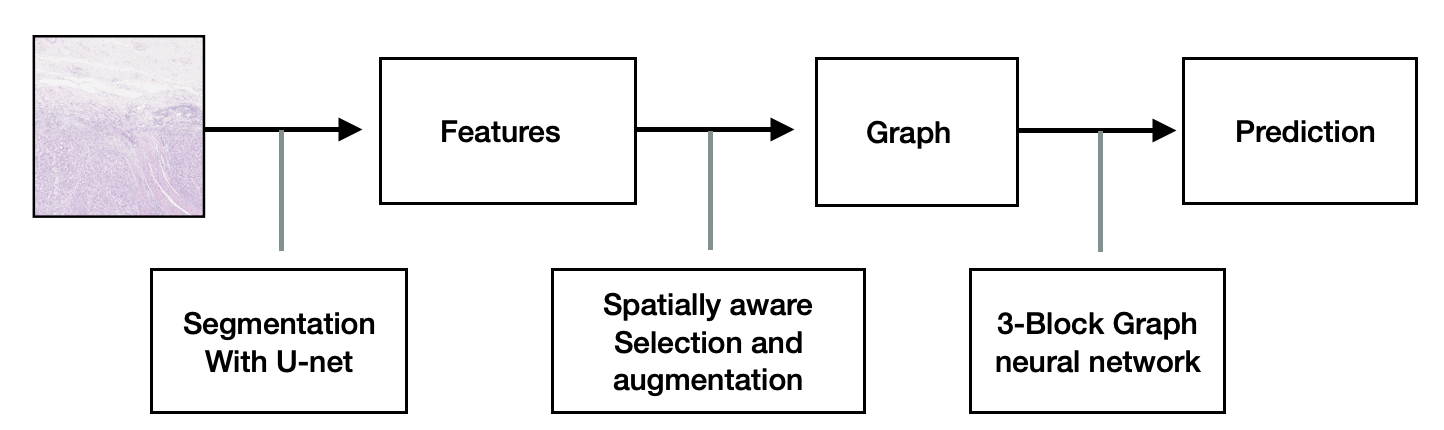
Figure 1: Overall carcinoma level prediction pipeline divided into three steps

3.1 From medical analysis to technical application

Cancer grading from a medical perspective requires thorough analysis of the cells within a whole tissue, and the challenge lies in interpreting a combination of the cell tissue type, tissue cut direction, cell overall distribution and abnormal structures, in addition complicated by non uniformity in the histopathology process.
Some of the observatory skills required to understand the complete image as one context and to differentiate between different grades are acquired by assistants through medical training, yet still hard for a technical application to understand.
Those challenges are amongst others: The understanding of ”empty spaces”, the implicit layer type determination and the overall grading logic for an image that contains partially different cancer level.

3.1.1 Interpretation of space and pattern

”Blank space” - in the image visible as ”white”, can either stand for missing tissue due to the extraction method or be a marker for a necrosis. While with the human eye there is a difference between a clean cut and a tissue decaying at the border of the cut, this feature is hard to understand from a machine learning point of view.
Further more glandular structures in the images pose a challenge to traditional visual analysis - Awan et al. (2017) have proposed to separately recognize glandular structures for cancer grading. This work assumes the opposite, namely that the graph representation in combination with the graph neural network can treat different structures for one cancer grade equally. This is enforced by design, as the graph representing the cell structures is locally dense, i.e. each cell is connected to each other cell, and as edge weights are applied in a locally constant manner, this means that the representation of cells around glandular structures can be topologically equivalent to a graph representing a muscular structure, if the number of cells per area is the same. For technical details see section 4.2 and 4.3.

3.1.2 Comparison to a ground truth pattern

Analysing the tissue layer type and the tissue cut direction, is crucial to differentiate between a normal and abnormal tissue. Cancer grading is not straight forward linearly related to the number of cells per image. Traditional convolutional neural networks work on a pixel wise evaluation of an image. The pipeline steps two and three however only use relational position, not absolute. Whether or not cell A is 5 more pixel to the left or the right should in no manner influence the network. This is only possible by building a graph structure based upon nodes with visual features only and passing the graph through a graph neural network.

3.1.3 Local vs Global evaluation

As a result of the different tissue types and layers per sample, the local cancer grading results for different regions are not in general identical, i.e. one sample might contain different grades at different areas. Which is why the graph neural network uses patching to evaluate the result of each patch locally and then reason on the overall grading system with a linear layer block, see section 4.4.4.

3.2 Pipeline for prediction

The complete pipeline from histopathology image to prediction consists of three steps, it starts with cell segmentation, which is then followed by cell graph augmentation, and concluded with level prediction through a graph neural network, see figure 1 for reference.
Step 1: Feature calculation This work uses a 5-layer U-net trained on cell segmentation images as originally proposed by Ronneberger et al. (2015). Nodes for the graph correspond to features of the cell segmentation provided by the Unet. Similar to Zhou et al. (2019), 16 different properties per segmented cell are used for each node.
Step 2A: Feature Selection Due to the high amount of cells per image, the selected number of cells are downsampled using distribution aware methods. For a fixed number of features, the selection uses random choices per area.
Step 2B: Graph Augmentation Those randomly downsampled features are then augmented into a graph. The graph’s node have 16 features each and the edges are determined using distribution based edge values. The edge value function is proportional to both the local distribution and the variance in distribution.
Step 3: Graph Neural Network The graph is analysed through a network consisting of three convolutional blocks and a prediction layer, where as each block consists of one GraphSAGE convolution, one pooling and one normalization layer, as shown in detail in figure 2.

4 Methodology

The pipeline is designed to be easily reproducible and lightweight during training: the cell segmentation is achieved with a conventional U-net Ronneberger et al. (2015), the feature selection and graph augmentation methods have linear complexity with respect to the number of nodes (i.e. cells), the graph neural network acts on vertices and edges in 3 convolutional blocks. In the following, the different technical details of those methods will be described:

4.1 Cell feature calculation

A U-net with 5 convolutional layers is used as described by the authors in Ronneberger et al. (2015). The resulting mask is processed to extract 16 features per cell instance, as proposed in Zhou et al. (2019). The first half of those are bounding box color features, the second half are segmentation mask based image features. In the experiments a study on the feature dimension has been executed.

4.2 Spatially aware feature selection

For a given segmentation map $s(i,j)$ of an image $I$ of dimension $w\times h$ at pixel position $(i,j)$ , let us define the distribution map as $D(i,j)$, which uses a regular 2D grid of dimension $dxd$ and counts the number of points per box. Then for any set of feature points $F=\{f_{0},\dots,f_{N}\}$ the corresponding distribution map for M feature points is

$$D_{M}(i,j)=\frac{M}{\|D\|}D(i,j)$$

where $\|\cdot\|$ stands for the $L_{1}$ matrix norm. Given the number of points per area through the distribution map $D_{M}(i,j)$, the features are augmented into a graph through random selection of nodes per area.

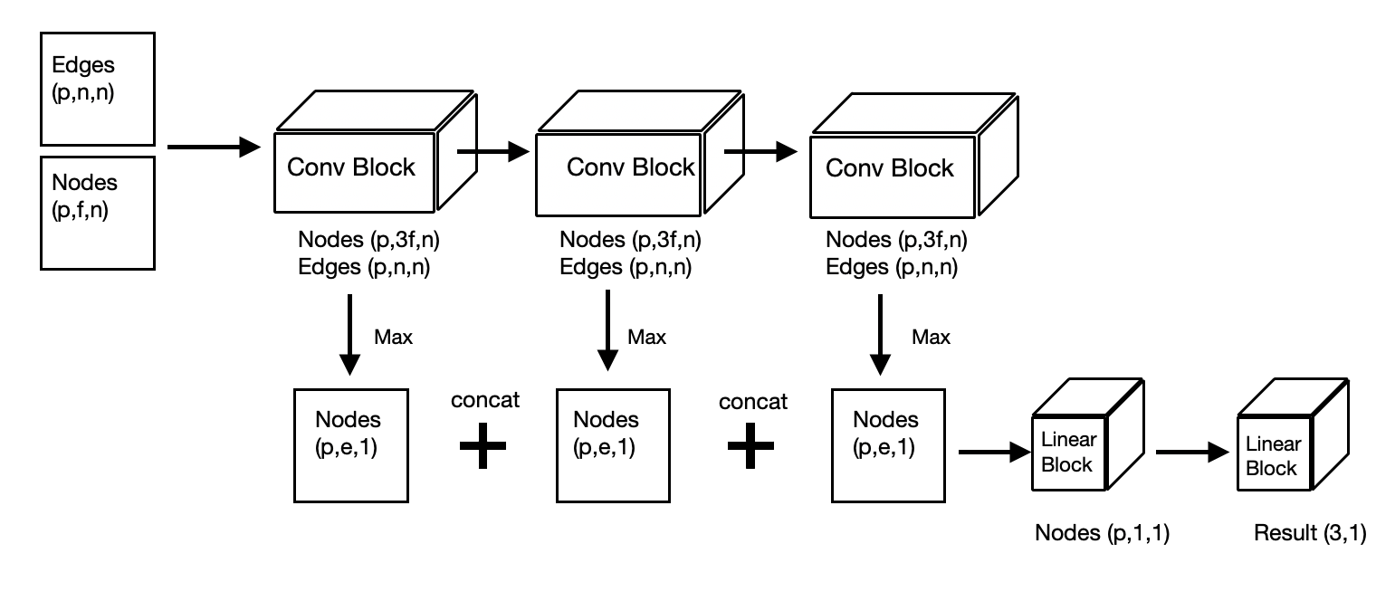
Figure 2: Architecture of graph network with dimensions of vertices where as p stands for the number of patches, f for the feature dimension, e for the embedded feature dimension and n for the number of nodes.

4.3 Spatially aware graph augmentation

For a given set of feature points $F=\{f_{0},\dots,f_{N}\}$ , the edge value between two feature points $f_{k},f_{m}$ and their corresponding coordinates $c_{k},c_{m}$ is defined as:

$$\begin{split}A_{k,m}&=\alpha(D_{M}(c_{k})+D_{M}(c_{m}))\\ &+\beta|D_{M}(c_{k})-D_{M}(c_{m})|\end{split}$$

where in this case $|\cdot|$ stands for the absolute value and $\alpha,\beta\in[0,1]$ are hyper parameters. Then the Matrix $A$ corresponds to the adjacency matrix of the augmented graph.

4.4 Cell Graph Neural Network architecture

This part of the pipeline leverages a graph neural network architecture that acts both on nodes and edges, applies pooling and normalization operations and classifies the graph into a category.
It consists of two parts, the graph modification and the graph classification. The graph modification network consists of graph convolution blocks that modify both edge and vertices stepwise. Each convolutional block consists of three graph convolutions that are concatenated, one pooling and one normalizing layer.
As a graph convolution propagation rule, this work uses GraphSAGE Hamilton et al. (2017):

$$h_{v}^{k}\leftarrow\sigma(\textbf{W}\cdot\textit{mean}(\{h_{v}^{k-1}\}\cup\{h_{u}^{k-1},\forall\textit{u}\in\textsl{N}\}))$$

where W is the edge weight matrix, N stands for the set of points lying in the direct neighborhood of node v, and h denotes the node’s feature with respect to node v and number of neighborhood jumps k. In this work only one hop convolutions will be applied.

4.4.1 Feature embedding

Many graph neural network architectures do not work with the original nodes i.e. features as input but upscale the dimensions, such as shown in work by Errica et al. (2019). Upscaling of the feature dimensions is done through increasing the output dimensions of the graph convolution respectively. Down scaling of features is executed by applying linear layers with the output dimension as the desired scaled size.
While each convolutional block contains three convolutions that are being concatenated, this would increase the feature dimensions by a factor equal to the number of concatenations. The feature dimension of each convolutional block is hence down scaled back to the original embedding dimension with a linear layer at each step. The convolutional block structure is simplified compared to the work proposed in Zhou et al. (2019), as the bi-directional LSTM is not used this way.

4.4.2 GNN normalization and stabilization

Graph neural networks suffer from the over smoothening of adjacency values. To fix this, the values of the adjacency matrix $A$ are reassigned after every block in the following manner as originally proposed by Chen et al. (2019):

$$A^{\prime}_{i,j}=\begin{cases}1-p\textbf{ if }i=j\\ \frac{p}{\sum_{i,i\neq j}A_{i,j}}\textbf{ if }i\neq j\\ \end{cases}$$ (1)

4.4.3 GNN pooling operations

The graph neural network leverages differential graph pooling Diffpool as originally described in Ying et al. (2018), which computes an assignment matrix seperating nodes into different clusters.

4.4.4 Graph patching

Given the original Graph G corresponding to the image I, the nodes and respective edges are split into patches according to the pixel position along each axis into two sections resulting in four patches. The patches are each treated as individual graphs during the convolutional blocks and are merged into one result at the end of the pipeline with a block of linear layers.
For sake of simplicity in our architecture sketch, it is assumed that the patches have same size or are padded with zeros if not. In practice different number of nodes per patch have been used, as the splitting method does not take number of nodes into account.
Instead of typically used batch norm, the graph convolutional layers’ outputs are stabilized with ”patch norm”.

5 Experiments

5.1 Preliminaries

All of the experiments are conducted on a single GPU per task. Many of the experiments take less than 20 GB of GPU Memory, some experiments on the single graph with high number of nodes take up to 46 GB. All experiments on work from this paper use less than 10 GB of CPU memory. Graph augmentation was implemented to work on multiple cores.
The neural network has been coded in PyTorch Paszke et al. (2019) and specifically PyTorch Geometric Fey and Lenssen (2019). For the cell segmentation the code available at Milesi (2020) has been used.

5.2 Data

The Unet for semantic segmentation of cells is trained on the training set of the colorectal cancer cell data set CoNSeP Graham et al. (2019), which contains 41 images with segmentation labels of resolution 1000x1000 pixel.
The graph neural network is trained on the Extended Colorectal Adenocarcinoma Dataset (abbreviated in this work with ECA) for Grading of Histology Images Shaban et al. (2020), which classifies 300 images from 178 different patients of resolutions around 5000x7000 pixel into three categories: no cancer , low level and high level. In order to enable comparisons to scores in previous works, the Colorectal Cancer Grading Dataset (CRC) ( Awan et al. (2017)) is used, which contains a subset of the Extended Colorectal Adenocarcinoma Dataset, in total 137 images from 38 different patients.

5.3 Feature calculation

For the semantic segmentation, the u-net is trained on 100 epochs on the CoNSeP training data set. The training and test split is provided with the data. The binary cross entropy with logits is used for training, together with a learning rate plateau scheduler and Root Mean Square Propagation. After those epochs, it overall achieves a dice test score of 75.60 out of 100. As the dice score heavily punishes segmentation areas larger than the labeled segmentation, this means that the segmented cells potentially are slightly larger than the ground truth. Cells in the training data and test data have a bounding of around 10x10 pixel to 20x20 pixel, with main variations in different images and small size variation only per one image. For a 10x10 sized bounding box, with a mask area smaller than 100 pixel, a dice score of around 75 corresponds to a cell of around 125 pixel area.

Table 1: Overview over the ECA (Shaban et al. (2020)) and CRC datasets (Awan et al. (2017)) used for cancer level prediction; the label split shows the distribution of samples among labels no grade, low grade, high grade and the fold split shows the number of samples per fold 1,2 and 3

Dataset	CRC	ECA
Samples	137	300
Label Split	71-31-35	120-120-60
Fold Split	45-46-46	100-100-100
Patients	38	178

5.4 Cancer Grading and Graph Network

Table 2: Overall best accuracy scores for different parameters, Accuracy and standard deviation values are provided in percentage

Method	CRC	ECA
CA-CNN Shaban et al. (2020)	$95.70\pm 3.04$	-
CGC Zhou et al. (2019)	$97.00\pm 1.10$	-
this work (CRC)	$99.26\pm 1.05$	-
this work (ECA)	$99.26\pm 0.66$	$99.33\pm 0.94$

In Table 2, it is shown that this work improves the accuracy of other works on this data set by around two percent on the CRC data set and the ECA data set. Parameter The normalization layer is being used with p = 0.4. The embedding dimension has been chosen to be 100, in some experiments 120. From the classification head, the first linear layer block contains three linear layers with dimensions 50,25,3 respectively. The patch classification layer contains two linear layers with dimensions 3 and 1. The learning rate has to be adjusted for each specific experiment but on average lies between 0.00005 and 0.00001 at initialization. The learning rate is scheduled with a plateau scheduler with respect to the accuracy
Evaluation criteria As training is executed using 3-fold cross validation, the evaluation for the complete pipeline is given in terms of the average and standard deviation of the last three accuracy values. The loss function used during training of the graph neural network is a smooth L1 loss.
Time estimations Training on the graph neural network including all necessary steps requires around 6-14h per model and configuration, with variations of several hours for usage of normalization layers and large graph sizes.

5.5 Ablation Studies

5.5.1 Patching versus one graph

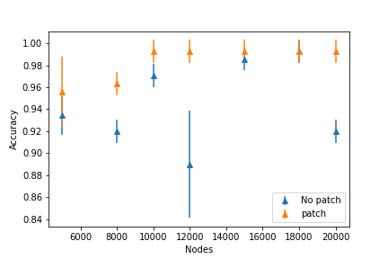
Figure 3: Comparison of accuracy scores with and without patching for different number of nodes on the CRC dataset

In figure 3, accuracy values for one graph per image vs. 4 graphs per image have been compared.
While one graph per image yields a straight forward classification score, separating the graph into patches and evaluating on those patches requires a classification head that decides on the overall label based on each patch. Evaluation results for a single graph are unstable over the selection of number of nodes for the augmentation and achieve in general lower accuracy than with four graphs per image.

5.5.2 Different cell segmentation features as input

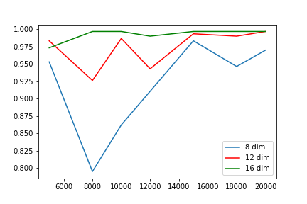
Figure 4: Change of accuracy for different feature dimensions 8,12,16 of nodes and different graph sizes for training on the ECA dataset

While this paper adapted the 16 cell segmentation features as in Zhou et al. (2019), a set of experiments have been conducted on using smaller amount of cell features from the segmentation. Of those features, the first half of them characterize the bounding box color and black and white values, while the second half of features characterizes the properties of the masked cell. Testing has been done on 8-dim feat input (only looking at bounding box based features) and 12 dim input with restricted segmentation features. While the stability inspected over smaller graphs decreases for lower feature dimensions, for a graph size of 16000 the accuracy values are observed to peak for all feature dimensions and differ by around 2 percent only.

6 Conclusion

In this work a stable and efficient graph neural network pipeline has been proposed to evaluate cancer grades. Experiments on parameters have shown that a stable architecture design and efficient pipeline can improve evaluation results.
Graph augmentation, just like image augmentation and text augmentation, has significant impact on the quality of the results. Compared to the state of the art, the pipeline accuracy results are improved by around two percent and the overall number of false predictions is decreased.
Further, experiments have been executed with respect to graph size and number of nodes, which shows that downsampling of graphs must not lead to a loss in accuracy. This would also possibly enable testing on devices and hardware with less available memory, as graph neural network training can be much more expensive than training of traditional neural networks.
Further, the author suggest that this pipeline has the potential to be used on other diseases related to histopathological image diagnosis.

7 Acknowledgement

The author would like to thank Dr. Anish Mohammed for this medical advice. Special thanks to Gregory Senay for his support during the writing process.

References

- Awan et al. (2017) Ruqayya Awan, Korsuk Sirinukunwattana, David Epstein, Samuel Jefferyes, Uvais Qidwai, Zia Aftab, Imaad Mujeeb, David Snead, and Nasir Rajpoot. Glandular morphometrics for objective grading of colorectal adenocarcinoma histology images. Scientific reports, 7(1):1–12, 2017.
- Chen et al. (2019) Zhao-Min Chen, Xiu-Shen Wei, Peng Wang, and Yanwen Guo. Multi-label image recognition with graph convolutional networks. In Proceedings of the IEEE Conference on Computer Vision and Pattern Recognition, pages 5177–5186, 2019.
- Dwivedi et al. (2020) Vijay Prakash Dwivedi, Chaitanya K Joshi, Thomas Laurent, Yoshua Bengio, and Xavier Bresson. Benchmarking graph neural networks. arXiv preprint arXiv:2003.00982, 2020.
- Errica et al. (2019) Federico Errica, Marco Podda, Davide Bacciu, and Alessio Micheli. A fair comparison of graph neural networks for graph classification. arXiv preprint arXiv:1912.09893, 2019.
- Fey and Lenssen (2019) Matthias Fey and Jan Eric Lenssen. Fast graph representation learning with pytorch geometric. arXiv preprint arXiv:1903.02428, 2019.
- Graham et al. (2019) Simon Graham, Quoc Dang Vu, Shan E Ahmed Raza, Ayesha Azam, Yee Wah Tsang, Jin Tae Kwak, and Nasir Rajpoot. Hover-net: Simultaneous segmentation and classification of nuclei in multi-tissue histology images. Medical Image Analysis, 58:101563, 2019.
- Hamilton et al. (2017) Will Hamilton, Zhitao Ying, and Jure Leskovec. Inductive representation learning on large graphs. In Advances in neural information processing systems, pages 1024–1034, 2017.
- Juarez et al. (2019) Antonio Garcia-Uceda Juarez, Raghavendra Selvan, Zaigham Saghir, and Marleen de Bruijne. A joint 3d unet-graph neural network-based method for airway segmentation from chest cts. In International Workshop on Machine Learning in Medical Imaging, pages 583–591. Springer, 2019.
- Lippoldt and Lavin (2020) Franziska Lippoldt and Alexander Lavin. Attention-sampling graph convolutional networks. submitted to Arxiv, 2020.
- Milesi (2020) Alexandre Milesi. Unet: semantic segmentation with pytorch, 2020. URL https://github.com/milesial/Pytorch-UNet.
- Morris et al. (2019) Christopher Morris, Martin Ritzert, Matthias Fey, William L Hamilton, Jan Eric Lenssen, Gaurav Rattan, and Martin Grohe. Weisfeiler and leman go neural: Higher-order graph neural networks. In Proceedings of the AAAI Conference on Artificial Intelligence, volume 33, pages 4602–4609, 2019.
- Paszke et al. (2019) Adam Paszke, Sam Gross, Francisco Massa, Adam Lerer, James Bradbury, Gregory Chanan, Trevor Killeen, Zeming Lin, Natalia Gimelshein, Luca Antiga, et al. Pytorch: An imperative style, high-performance deep learning library. In Advances in neural information processing systems, pages 8026–8037, 2019.
- Ronneberger et al. (2015) Olaf Ronneberger, Philipp Fischer, and Thomas Brox. U-net: Convolutional networks for biomedical image segmentation. In International Conference on Medical image computing and computer-assisted intervention, pages 234–241. Springer, 2015.
- Shaban et al. (2020) Muhammad Shaban, Ruqayya Awan, Muhammad Moazam Fraz, Ayesha Azam, Yee-Wah Tsang, David Snead, and Nasir M Rajpoot. Context-aware convolutional neural network for grading of colorectal cancer histology images. IEEE Transactions on Medical Imaging, 2020.
- Siegel et al. (2020) Rebecca L Siegel, Kimberly D Miller, Ann Goding Sauer, Stacey A Fedewa, Lynn F Butterly, Joseph C Anderson, Andrea Cercek, Robert A Smith, and Ahmedin Jemal. Colorectal cancer statistics, 2020. CA: a cancer journal for clinicians, 2020.
- Wolf et al. (2018) Andrew MD Wolf, Elizabeth TH Fontham, Timothy R Church, Christopher R Flowers, Carmen E Guerra, Samuel J LaMonte, Ruth Etzioni, Matthew T McKenna, Kevin C Oeffinger, Ya-Chen Tina Shih, et al. Colorectal cancer screening for average-risk adults: 2018 guideline update from the american cancer society. CA: a cancer journal for clinicians, 68(4):250–281, 2018.
- Xu et al. (2018) Keyulu Xu, Weihua Hu, Jure Leskovec, and Stefanie Jegelka. How powerful are graph neural networks? arXiv preprint arXiv:1810.00826, 2018.
- Ying et al. (2018) Zhitao Ying, Jiaxuan You, Christopher Morris, Xiang Ren, Will Hamilton, and Jure Leskovec. Hierarchical graph representation learning with differentiable pooling. In Advances in neural information processing systems, pages 4800–4810, 2018.
- Yu et al. (2019) Bing Yu, Haoteng Yin, and Zhanxing Zhu. St-unet: A spatio-temporal u-network for graph-structured time series modeling. arXiv preprint arXiv:1903.05631, 2019.
- Zhou et al. (2019) Yanning Zhou, Simon Graham, Navid Alemi Koohbanani, Muhammad Shaban, Pheng-Ann Heng, and Nasir Rajpoot. Cgc-net: Cell graph convolutional network for grading of colorectal cancer histology images. In The IEEE International Conference on Computer Vision (ICCV) Workshops, 2019.