Unsupervised Point Cloud Pre-training via Occlusion Completion

Abstract

We describe a simple pre-training approach for point clouds. It works in three steps: 1. Mask all points occluded in a camera view; 2. Learn an encoder-decoder model to reconstruct the occluded points; 3. Use the encoder weights as initialisation for downstream point cloud tasks. We find that even when we pre-train on a single dataset (ModelNet40), this method improves accuracy across different datasets and encoders, on a wide range of downstream tasks. Specifically, we show that our method outperforms previous pre-training methods in object classification, and both part-based and semantic segmentation tasks. We study the pre-trained features and find that they lead to wide downstream minima, have high transformation invariance, and have activations that are highly correlated with part labels. Code and data are available at: https://github.com/hansen7/OcCo

1 Introduction

There has been a flurry of exciting new point cloud models for object detection [27, 52, 64] and segmentation [22, 26, 57, 65]. These methods rely on large scale point cloud datasets that are labelled. Unfortunately, labelling point clouds is challenging for a number of reasons: (1) Point clouds can be sparse, occluded, and at low resolutions, making the identity of points ambiguous; (2) Datasets that are not sparse can easily reach hundreds of millions of points (e.g., small dense point clouds for object classification [63] and large vast point clouds for reconstruction [66]); (3) Labelling individual points or drawing 3D bounding boxes are both more time-consuming and error-prone than labelling 2D images [50]. These challenges have impeded the deployment of point cloud models into new real world settings where labelled data is scarce.

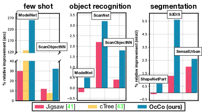
Figure 1: The relative improvement over random initialisation of multiple pre-training methods: Jigsaw [42], cTree [44], and OcCo (ours) for various downstream tasks.

However, current 3D sensing modalities (i.e., 3D scanners, stereo cameras, lidars) have enabled the creation of large unlabelled repositories of point cloud data [13, 41]. This has inspired a recent line of work on unsupervised pre-training methods to learn point cloud model initialisation. Initial work used latent generative models such as generative adversarial networks (GANs) [1, 14, 54] and autoencoders [15, 29, 59]. These have been recently outperformed by self-supervised objectives [42, 56, 2, 44, 20, 61].

Inspired by this recent line of work, we propose Occlusion Completion (OcCo), an unsupervised pre-training method that consists of: (a) a mechanism to generate masked point clouds via view-point occlusions, and (b) a completion task to reconstruct the occluded point cloud. The idea of occlusion+completion is grounded in three observations: (1) A pre-trained model that is accurate at completing occluded point clouds needs to understand spatial and semantic properties of these point clouds. (2) 3D scene completion [45, 9, 19] has been shown to be a useful auxiliary task for learning representations for visual localisation [43]. (3) Mask-based completion tasks have become the de facto standard for learning pre-trained representations in natural language processing [11, 32, 36] and are widely used in pre-training for images [35] and graphs [24].

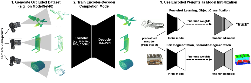
Figure 2: Overview of OcCo. 1. Take any point cloud dataset and generate occluded objects for each input by (a) randomly sampling a camera view-point, and (b) removing points hidden from that view-point (for all experiments we use the same occluded dataset generated from ModelNet40); 2. Train an encoder-decoder model to complete the occluded point clouds (the encoder can be any model that learns representations of point clouds, the decoder can be any completion model); 3. Use the learned encoder weights as initialisation for any downstream task (e.g., few-shot learning, object classification, part/semantic segmentation). We show that OcCo outperforms a variety of pre-training methods across multiple models and tasks.

We demonstrate that pre-training on a single object-level dataset (ModelNet40) can improve the performance of a range of downstream tasks, even on completely different datasets. Specifically we find that OcCo has the following properties compared to other initialisation techniques: 1) Improved sample efficiency in few-shot learning experiments; 2) Improved generalisation in object classification, object part segmentation, and semantic segmentation; 3) Wider local minima found after fine-tuning; 4) More semantically meaningful representations as described via network dissection [4, 5]; 5) Better clustering quality under jittering, translation, and rotation transformations.

2 Related Work

Unsupervised pre-training is gaining popularity due to its success in many problem settings, such as natural language understanding [11, 32], object detection [8, 16], graph learning [23, 24], and visual localisation [43]. Currently, the two most common unsupervised pre-training methods for point clouds are based on (i) generative modelling, and (ii) self-supervised learning. Work in generative modelling includes models based on generative adversarial networks (GANs) [54, 1, 14], autoencoders [15, 29, 59], normalizing flows [58], and approximate convex decomposition [12].

However, generative models for unsupervised pre-training on point clouds have recently been outperformed by self-supervised approaches [42, 44, 56]. These approaches work by learning to predict key geometric properties of point clouds that are invariant across datasets. Specifically, [42] propose a pre-training procedure based on rearranging permuted point clouds. It works by splitting a point cloud into $k^{3}$ voxels, randomly permuting the voxels, and then training a model to predict the original voxel location of each point. The idea is that the pre-trained model implicitly learns about the geometric structure of point clouds by learning this rearrangement. However, there are two key issues with this objective: 1. The voxel representation is not permutation invariant. Thus, the model could learn very different representations if point clouds are rotated or translated; 2. Point clouds generated from real objects and scenes will have very different structure from randomly permuted clouds, so it is unclear why pre-trained weights that are accurate at rearrangement will be good initialisation for object classification or segmentation models. Another work [44] uses cover trees [6] to hierarchically partition points for few-shot learning. They then train a model to classify each point to their assigned partitions. However, because cover trees are designed for fast nearest neighbour search, they may arbitrarily partition semantically-contiguous regions of point clouds (e.g., airplane wings, car tires) into different regions of the hierarchy, and so ignore key point cloud geometry. A third work, PointContrast [56], uses contrastive learning to pre-train weights for point clouds of scenes. Their method uses known point-wise correspondences between different views of a complete 3D scene. These point-wise correspondences require post-processing the data by registering different depth maps into a single 3D scene. Thus, their method can only be applied to static scenes that have been registered, limiting the applicability of the approach: we leave a comparison between OcCo and PointContrast to future work. In what follows we will show that unsupervised pre-training based on a simple self-supervised objective: completing occluded point clouds, produces weights that outperform [42] and [44] on downstream tasks.

Completing 3D shapes to learn model initialisations is not new, [43] used scene completion [45, 9, 19] as a pre-training task to initialise 3D voxel descriptors for visual localisation. To do so, they generated partial voxelised scenes based on depth images and trained a variational autoencoder for completion. Differently, our focus is to describe a technique to learn an initialisation for point cloud models. Our aim is for this pre-trained initialisation to improve a variety of downstream tasks including few-shot learning, object classification, and segmentation, on a variety of datasets.

3 Occlusion Completion

The overall idea of our approach is shown in Figure 2. Our observation is that by occluding point clouds based on different view-points then learning a model to complete them, the weights of the completion model can be used as initialisation for downstream tasks (e.g., classification, segmentation). This approach not only improves accuracy in few-shot learning settings but also the final generalisation accuracy in fully-supervised tasks.

Throughout we define point clouds $\mathcal{P}$ as sets of points in 3D Euclidean space, $\mathcal{P}=\{p_{1},p_{2},...,p_{n}\}$, where each point $p_{i}$ is a vector of both coordinates $(x_{i},y_{i},z_{i})$ and other features (e.g. colour and normal). We begin by describing the components that make up our occlusion mapping $o(\cdot)$. Then we detail how to learn a completion model $c(\cdot)$, giving pseudo-code and the architectural details in the appendix.

3.1 Generating Occlusions

We define a randomised occlusion mapping $o:\mathbb{P}\rightarrow\mathbb{P}$ (where $\mathbb{P}$ is the space of all point clouds) from a full point cloud $\mathcal{P}$ to an occluded point cloud $\tilde{\mathcal{P}}$. This mapping constructs $\tilde{\mathcal{P}}$ by removing points from $\mathcal{P}$ that cannot be seen from a particular view-point. This is accomplished in three steps: (1) A projection of the complete point cloud (in a world reference frame) into the coordinates of a camera reference frame (which specifies the view-point); (2) Identification of the points that are occluded in the camera view-point; (3) A projection of the points back from the camera reference frame to the world reference frame.

Viewing the point cloud from a camera.

A camera defines a projection from a 3D world reference frame into a distinctive 3D camera reference frame. It does so by specifying a camera model and a camera view-point from which the projection occurs. While any camera model can be used, for illustration consider the simplest camera model: the pinhole camera. View-point projection for the pinhole camera is given by a simple linear equation:

$$\begin{bmatrix}x_{\text{cam}}\\ y_{\text{cam}}\\ z_{\text{cam}}\\ \end{bmatrix}\!\!=\!\!\underbrace{\vphantom{\left[\begin{array}[]{ccc|c}r_{1}&r_{2}&r_{3}&t_{1}\\ r_{4}&r_{5}&r_{6}&t_{2}\\ r_{7}&r_{8}&r_{9}&t_{3}\end{array}\right]}\begin{bmatrix}f&\gamma&w/2\\ 0&f&h/2\\ 0&0&1\end{bmatrix}}_{\begin{subarray}{c}\text{intrinsic}\\ [\;\;\;\;\mathbf{K}\;\;\;\;]\end{subarray}}\underbrace{\left[\begin{array}[]{ccc|c}r_{1}&r_{2}&r_{3}&t_{1}\\ r_{4}&r_{5}&r_{6}&t_{2}\\ r_{7}&r_{8}&r_{9}&t_{3}\end{array}\right]}_{\vbox{\Let@\restore@math@cr\default@tag\halign{\hfil$\m@th\scriptstyle#$&$\m@th\scriptstyle{}#$\hfil\cr\text{rotation }&|\text{ translation}\\ [\;\;\;\mathbf{R}\;\;\;\;\;&|\;\;\;\;\;\;\;\mathbf{t}\;\;\;\;\;]\crcr}}}\begin{bmatrix}x\\ y\\ z\\ 1\end{bmatrix}$$ (9)

In the above, $(x,y,z)$ are the original point cloud coordinates (in a world reference), the camera viewpoint is described by the concatenation of a rotation matrix ($r$ entries) with a translation vector ($t$ entries) describing the camera view-point, and the final matrix is the camera intrinsics ($f$ specifies the camera focal length, $\gamma$ is the skewness between the $x$ and $y$ axes in the camera, and $w,h$ are the width and height of the camera image). Given these, the final coordinates $(x_{\text{cam}},y_{\text{cam}},z_{\text{cam}})$ are the positions of the point in the camera reference frame. We will refer to the intrinsic matrix as $\mathbf{K}$ and the rotation/translation matrix as $[\mathbf{R}|\mathbf{t}]$.

Determining occluded points.

We can think of the point $(x_{\text{cam}},y_{\text{cam}},z_{\text{cam}})$ in multiple ways: (a) a 3D point in the camera reference frame; (b) a 2D pixel with coordinates $(fx_{\text{cam}}/z_{\text{cam}},fy_{\text{cam}}/z_{\text{cam}})$ with a depth of $z_{\text{cam}}$. In this way, some 2D points resulting from the projection may be occluded by others if they have the same pixel coordinates, but appear at a farther depth. To determine which points are occluded, we first use Delaunay triangulation to reconstruct a polygon mesh, then we remove the points which belong to the hidden surfaces that are determined via z-buffering [47].

Mapping back from camera frame to world frame.

Once occluded points are removed, we re-project the point cloud to the original world reference frame, via the inverse transformation of eq. (9). Thus, the randomised occlusion mapping $o(\cdot)$ is constructed as follows. Fix an initial point cloud $\mathcal{P}$. Given a camera intrinsics matrix $\mathbf{K}$, sample rotation/translation matrices $[[\mathbf{R}_{1}|\mathbf{t}_{1}],\ldots,[\mathbf{R}_{V}|\mathbf{t}_{V}]]$, where $V$ is the number of views. For each view $v\in[V]$, project $\mathcal{P}$ into the camera frame of that view-point using eq. (9), find occluded points and remove them, then map all other points back to the world reference using its inverse. This yields the final occluded point cloud $\tilde{\mathcal{P}}_{v}$ for each view-point $v\in[V]$.

3.2 The Completion Task

Given an occluded point cloud $\tilde{\mathcal{P}}$ produced by $o(\cdot)$, the goal of the completion task is to learn a completion mapping $c:\mathbb{P}\rightarrow\mathbb{P}$ from $\tilde{\mathcal{P}}$ to a completed point cloud $\hat{\mathcal{P}}$. A completion mapping is accurate w.r.t. loss $\ell(\cdot,\cdot)$ if $\mathbb{E}_{\tilde{\mathcal{P}}\sim o({\mathcal{P}})}\ell(c(\tilde{\mathcal{P}}),{\mathcal{P}})\rightarrow 0$. The structure of the completion model $c(\cdot)$ is an “encoder-decoder” network [10, 48, 51, 60]. The encoder maps an occluded point cloud to a vector, and the decoder completes the point cloud. After pre-training, the encoder weights can be used as initialisation for downstream tasks. In the appendix we give pseudocode for OcCo. We describe details of the completion model architecture in the following section.

4 Experiments

In this section, we present the setup of pre-training (Section 4.1) and downstream fine-tuning (Section 4.2). Then, the results of few-shot learning, object classification, part and semantic segmentation are shown in Section 4.3.

4.1 OcCo Pre-Training Setup

Dataset.

For all experiments, we use ModelNet40 [55] as the pre-training dataset. ModelNet40 includes 12,311 synthesised CAD objects from 40 categories, and the dataset is divided into 9,843/2,468 objects for training and testing, respectively. We construct a pre-training dataset using the training set. Occluded point clouds are generated with camera intrinsic parameters {$f$=1000, $\gamma$=0, $\omega$=1600, $h$=1200}. For each point cloud, we randomly select 10 viewpoints, where the yaw, pitch and roll angles are uniformly chosen between 0 and 2$\pi$, and the translation is set as zero.

Architecture.

As described above, our pre-training completion model $c(\cdot)$ is an encoder-decoder model. To showcase that our pre-training method is agnostic to architectures, we choose three different encoders, including PointNet [37], PCN [60] and DGCNN [53]. These encoders map an occluded point cloud into a 1024-dimensional vector. We adapt the folding-based decoder from [60] to complete an occluded point cloud in two steps. The decoder first outputs a coarse shape consisting of 1024 points, $\hat{\mathcal{P}}_{coarse}$, then warps a 4$\times$4 2D grid around each point in $\hat{\mathcal{P}}_{coarse}$ to reconstruct a fine shape, $\hat{\mathcal{P}}_{fine}$, which consists of 16384 points. We use the Chamfer Distance (CD) as a closeness measure between prediction $\hat{\mathcal{P}}$ and ground-truth $\mathcal{P}$:

$$\begin{split}\mathrm{CD}(\hat{\mathcal{P}},\mathcal{P})=&\\ \frac{1}{|\hat{\mathcal{P}}|}&\sum_{\hat{x}\in\hat{\mathcal{P}}}\min_{x\in\mathcal{P}}||\hat{x}-x||_{2}+\frac{1}{|\mathcal{P}|}\sum_{x\in\mathcal{P}}\min_{\hat{x}\in\hat{\mathcal{P}}}||x-\hat{x}||_{2}.\end{split}$$ (10)

The loss of the completion model is a weighted sum of the Chamfer distances on the coarse and fine shapes:

$$\ell:=\mathrm{CD}(\hat{\mathcal{P}}_{coarse},\mathcal{P}_{coarse})+\alpha\mathrm{CD}(\hat{\mathcal{P}}_{fine},\mathcal{P}_{fine}).$$ (11)

Hyperparameters.

We use the Adam [25] optimiser with no weight decay (L2 regularisation). The learning rate is set to 1e-4 initially and is decayed by 0.7 every 10 epochs. We pre-train the models for 50 epochs. The batch size is 32, and the momentum of batch normalisation is 0.9. The coefficient $\alpha$ in eq. (11) is set as 0.01 for the first 10000 training iterations, then increased to 0.1, 0.5 and 1.0 after 10000, 20000 and 50000 training steps, respectively.

4.2 Fine-Tuning Setup

Few-shot learning.

Few-shot learning (FSL) aims to train accurate models with very limited data. A typical setting of FSL is “$K$-way $N$-shot”. During training, $K$ classes are randomly selected, and each category contains $N$ samples. The trained models are then evaluated on the objects from the test split. We compare OcCo with Jigsaw [42], and cTree [44] since it outperforms previous unsupervised methods [1, 54, 62, 59] as well as supervised variants [38, 30, 37, 53]. We follow the same setting as cTree, where we pre-train the models in a “$K$-way $N$-shot” configuration on ModelNet40, before evaluating on ModelNet40 and ScanObjectNN.

Object classification.

Given an object represented by a set of points, object classification predicts the class that the object belongs to. We use three benchmarks: ModelNet40 [55], ScanNet10 [39] and ScanObjectNN [49], the dataset statistics are summarised in Table 1. The latter two are more challenging since they consist of occluded objects from the real-world indoor scans. We use the same settings as [37, 53] for fine-tuning. Specifically, for PCN and PointNet, we use the Adam optimizer with an initial learning rate of 1e-3, and the learning rate is decayed by 0.7 every 20 epochs with the minimum value 1e-5. For DGCNN, we use the SGD optimizer with momentum 0.9 and weight decay 1e-4. The learning rate starts from 0.1 and then decays using cosine annealing [31] with the minimum value 1e-3. We use dropout [46] in the fully connected layers before the softmax output layer. The dropout rate is set to 0.7 for PointNet and PCN and is set to 0.5 for DGCNN. For all three models, we train them for 200 epochs with batch size 32. We report the test results based on three runs in Table 3.

Table 1: Statistics of classification datasets

Name	Type	# Class	# Training/Testing
ModelNet	synthesised	40	9,843 / 2,468
ScanNet	real scanned	10	6,110 / 1,769
ScanObjectNN	real scanned	15	2,304 / 576

Part segmentation.

Part segmentation is a challenging fine-grained 3D recognition task. The mission is to predict the part category label (e.g., chair leg, cup handle) of each point for a given object. To evaluate the effectiveness of OcCo pre-training, we use ShapeNetPart [3] benchmark, which contains 16,881 objects from 16 categories and has 50 parts in total. Each object is represented by 2048 points. For PCN and PointNet, we use the Adam optimizer with an initial learning rate of 1e-3, and the learning rate is decayed by 0.5 every 20 epochs with the minimum value 1e-5. For DGCNN, we use an SGD optimizer with momentum 0.9 and weight decay 1e-4. The learning rate starts from 0.1 and then decays using cosine annealing [31] with the minimum value 1e-3. We train the models for 250 epochs with batch size 16. We use the same post-processing during testing as [37] and report the results over three runs in Table 4.

Semantic segmentation.

Semantic segmentation predicts the semantic object category of each point under an indoor/outdoor scene. We use S3DIS benchmark [3] for indoor scene segmentation and SensatUrban benchmark [21] for outdoor scene segmentation. S3DIS contains 3D scans collected via Matterport scanners in 6 different places, encompassing 271 rooms and 13 semantic classes. While SensatUrban consists of over three billion annotated points, covering large areas in a total of 7.6 km² from three UK cities (Birmingham, Cambridge, and York). Each point in SensatUrban is labelled as one of 13 semantic classes. We use the same pre-processing, post-processing and training settings as  [37, 53]. Each point is described by a 9-dimensional vector (coordinates, RGBs and normalised location). We train all the models for 100 epochs with batch size 24. We report the results based on three runs in Table 5.

Table 2: Few-shot learning results. We report mean and standard error over 10 runs and bold the best results.

Baseline	5-way		10-way
	10-shot	20-shot	10-shot	20-shot
	ModelNet40
PointNet, Rand	52.0$\pm$3.8	57.8$\pm$4.9	46.6$\pm$4.3	35.2$\pm$4.8
PointNet, Jigsaw	66.5$\pm$2.5	69.2$\pm$2.4	56.9$\pm$2.5	66.5$\pm$1.4
PointNet, cTree	63.2$\pm$3.4	68.9$\pm$3.0	49.2$\pm$1.9	50.1$\pm$1.6
PointNet, OcCo	89.7$\pm$1.9	92.4$\pm$1.6	83.9$\pm$1.8	89.7$\pm$1.5
DGCNN, Rand	31.6$\pm$2.8	40.8$\pm$4.6	19.9$\pm$2.1	16.9$\pm$1.5
DGCNN, Jigsaw	34.3$\pm$1.3	42.2$\pm$3.5	26.0$\pm$2.4	29.9$\pm$2.6
DGCNN, cTree	60.0$\pm$2.8	65.7$\pm$2.6	48.5$\pm$1.8	53.0$\pm$1.3
DGCNN, OcCo	90.6$\pm$2.8	92.5$\pm$1.9	82.9$\pm$1.3	86.5$\pm$2.2
	ScanObjectNN
PointNet, Rand	57.6$\pm$2.5	61.4$\pm$2.4	41.3$\pm$1.3	43.8$\pm$1.9
PointNet, Jigsaw	58.6$\pm$1.9	67.6$\pm$2.1	53.6$\pm$1.7	48.1$\pm$1.9
PointNet, cTree	59.6$\pm$2.3	61.4$\pm$1.4	53.0$\pm$1.9	50.9$\pm$2.1
PointNet, OcCo	70.4$\pm$3.3	72.2$\pm$3.0	54.8$\pm$1.3	61.8$\pm$1.2
DGCNN, Rand	62.0$\pm$5.6	67.8$\pm$5.1	37.8$\pm$4.3	41.8$\pm$2.4
DGCNN, Jigsaw	65.2$\pm$3.8	72.2$\pm$2.7	45.6$\pm$3.1	48.2$\pm$2.8
DGCNN, cTree	68.4$\pm$3.4	71.6$\pm$2.9	42.4$\pm$2.7	43.0$\pm$3.0
DGCNN, OcCo	72.4$\pm$1.4	77.2$\pm$1.4	57.0$\pm$1.3	61.6$\pm$1.2

Table 3: Overal accuracy on 3D object classification benchmarks. We reported the mean and standard error over three runs.

Dataset	PointNet			PCN			DGCNN
	Random	Jigsaw	OcCo	Random	Jigsaw	OcCo	Random	Jigsaw	OcCo
ModelNet	89.2$\pm$0.1	89.6$\pm$0.1	90.1$\pm$0.1	89.3$\pm$0.1	89.6$\pm$0.2	90.3$\pm$0.2	92.5$\pm$0.4	92.3$\pm$0.3	93.0$\pm$0.2
ScanNet	76.9$\pm$0.2	77.2$\pm$0.2	78.0$\pm$0.2	77.0$\pm$0.3	77.9$\pm$0.3	78.2$\pm$0.3	76.1$\pm$0.7	77.8$\pm$0.5	78.5$\pm$0.3
ScanObjectNN	73.5$\pm$0.5	76.5$\pm$0.4	80.0$\pm$0.2	78.3$\pm$0.3	78.2$\pm$0.1	80.4$\pm$0.2	82.4$\pm$0.4	82.7$\pm$0.8	83.9$\pm$0.4

Table 4: Overall accuracy and intersection of union (mIoU) on ShapeNetPart. We reported the mean and ste over three runs.

	PointNet			PCN			DGCNN
	Random	Jigsaw	OcCo	Random	Jigsaw	OcCo	Random	Jigsaw	OcCo
OA (%)	92.8$\pm$0.9	93.1$\pm$0.5	93.4$\pm$0.7	92.3$\pm$1.0	92.6$\pm$0.9	93.0$\pm$0.9	92.2$\pm$0.9	92.7$\pm$0.9	94.4$\pm$0.7
mIoU (%)	82.2$\pm$2.4	82.2$\pm$2.8	83.4$\pm$1.9	81.3$\pm$2.6	81.2$\pm$2.9	82.3$\pm$2.4	84.4$\pm$1.2	84.3$\pm$1.2	85.0$\pm$1.0

Table 5: Overall accuracy (OA) and mean intersection of union (mIoU) on the S3DIS across six folds over three runs.

	PointNet			PCN			DGCNN
	Rand	Jigsaw	OcCo	Rand	Jigsaw	OcCo	Rand	Jigsaw	OcCo
OA (%)	78.2$\pm$0.7	80.1$\pm$1.2	82.0$\pm$1.0	82.9$\pm$0.9	83.7$\pm$0.7	85.1$\pm$0.5	83.7$\pm$0.7	84.1$\pm$0.7	84.6$\pm$0.5
mIoU (%)	47.0$\pm$1.4	52.6$\pm$1.9	54.9$\pm$1.0	51.1$\pm$2.4	52.2$\pm$1.9	53.4$\pm$2.1	54.9$\pm$2.1	55.6$\pm$1.4	58.0$\pm$1.7

Table 6: Overall point accuracy (OA), mean class accuracy (mAcc) and mean class intersection of union (mIoU) on SensatUrban. We reported the mean and standard error over three runs. We use the same preprocess procedures as PointNet.

	OA(%)	mAcc(%)	mIoU(%)	ground	veg	building	wall	bridge	parking	rail	traffic	street	car	footpath	bike	water
PointNet	86.29	53.33	45.10	80.05	93.98	87.05	23.05	19.52	41.80	3.38	43.47	24.20	63.43	26.86	0.00	79.53
PointNet-Jigsaw	87.38	56.97	47.90	83.36	94.72	88.48	22.87	30.19	47.43	15.62	44.49	22.91	64.14	30.33	0.00	77.88
PointNet-OcCo	87.87	56.14	48.50	83.76	94.81	89.24	23.29	33.38	48.04	15.84	45.38	24.99	65.00	27.13	0.00	79.58
PCN	86.79	57.66	47.91	82.61	94.82	89.04	26.66	21.96	34.96	28.39	43.32	27.13	62.97	30.87	0.00	80.06
PCN-Jigsaw	87.32	57.01	48.44	83.20	94.79	89.25	25.89	19.69	40.90	28.52	43.46	24.78	63.08	31.74	0.00	84.42
PCN-OcCo	86.90	58.15	48.54	81.64	94.37	88.21	25.43	31.54	39.39	22.02	45.47	27.60	65.33	32.07	0.00	77.99
DGCNN	87.54	60.27	51.96	83.12	95.43	89.58	31.84	35.49	45.11	38.57	45.66	32.97	64.88	30.48	0.00	82.34
DGCNN-Jigsaw	88.65	60.80	53.01	83.95	95.92	89.85	30.05	43.59	46.40	35.28	49.60	31.46	69.41	34.38	0.00	80.55
DGCNN-OcCo	88.67	61.35	53.31	83.64	95.75	89.96	29.22	41.47	46.89	40.64	49.72	33.57	70.11	32.35	0.00	79.74

4.3 Fine-Tuning Results

Few-shot learning.

We report the experimental results on few-shot learning in Table 2. We colour the best results with blue for each encoder and bold the overall best score for each dataset. We use the same colouring scheme in all subsequent results. We find that OcCo outperforms both few-shot baselines Jigsaw [42] and cTree [44] in-domain (ModelNet40) and cross-domain (ScanObjectNN). We believe this is due to the fact that the occlusions OcCo generates will be due to the geometric structure of the object, whereas the voxel permutations of [42] and the cover tree partitioning of [44] may destroy aspects of this structure.

Object classification.

Table 3 compares OcCo with random and Jigsaw [42] initialisation on object classification. We show that OcCo-initialised models outperform these baselines on all datasets. OcCo performs well not only on the in-domain dataset (ModelNet), but also on cross-domain datasets (ScanNet and ScanObjectNN). The improvements are consistent across the three encoders. In the following section we will provide one explanation: the local minima found after fine-tuning an OcCo-based initialisation appear to be wider than those found using other initialisations.

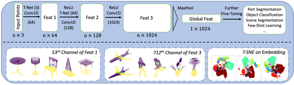
Figure 3: Visualisation on the learned features by OcCo-PointNet.

Object part segmentation.

Table 4 compares OcCo-initialisation with random and Jigsaw [42] initialisation on object part segmentation. We observe that OcCo-initialised models outperform the others in terms of overall accuracy and mean class IoU. These results are consistent across various encoders. We further analyse why OcCo helps the encoders better recognise the object parts with feature visualisation and concept detection in Section 5.

Semantic segmentation.

We compare random, Jigsaw and OcCo initialisation on both indoor and outdoor semantic segmentation tasks. For S3DIS, we evaluate the trained models using $6$-fold cross-validation following [3], and report the scores in Table 5. It is clear that OcCo-initialised models outperform random and Jigsaw-initialised ones. For SensatUrban, we report the scores in Table 6. We observe that OcCo outperforms random initialisation and Jigsaw initialisation for semantic categories that are included in the pre-training dataset, such as cars. For classes that are not included in ModelNet40, OcCo is competitive with the other methods. This makes sense as the geometries of these objects are likely not well understood by the learned initialisations. Ultimately, we find it encouraging that OcCo which learns representations at the object-level can still improve generalisation on segmentation on outdoor scenes.

5 Analysis

In this section, we first show that OcCo pre-training leads to a fine-tuned model that converges to a local minimum that is flatter than other initialisations. Then we evaluate the learned representations from OcCo with feature visualisation, semantic concept detection and unsupervised mutual information. The analysis demonstrates that OcCo can learn rich and discriminative point cloud features.

Visualisation of optimisation landscape.

We follow the same procedure of [28] to visualise the loss landscapes of random, Jigsaw and OcCo initialised PointNet in Figure 4. All three models are fine-tuned on ScanObjectNN with the training settings described in Section 4.2. For visualisation, we use two random vectors, $\boldsymbol{\delta}$ and $\boldsymbol{\eta}$, to perturb the fine-tuned parameters $\boldsymbol{\theta}^{*}$ and obtain corresponding loss values. The 2D plot $f(\alpha,\beta)$ is defined as:

$$f(\alpha,\beta)=\mathcal{L}\left(\boldsymbol{\theta}^{*}+\alpha\boldsymbol{\delta}+\beta\boldsymbol{\eta}\right)$$ (12)

where each filter in $\boldsymbol{\delta}$ and $\boldsymbol{\eta}$ is normalised w.r.t the corresponding filter in $\boldsymbol{\theta}^{*}$. $\alpha$ and $\beta$ have the same ranges of $[-1,1]$. We observe that the model with OcCo pre-training can converge to a flatter local minimum, which is known to have better generalisation [7, 18].

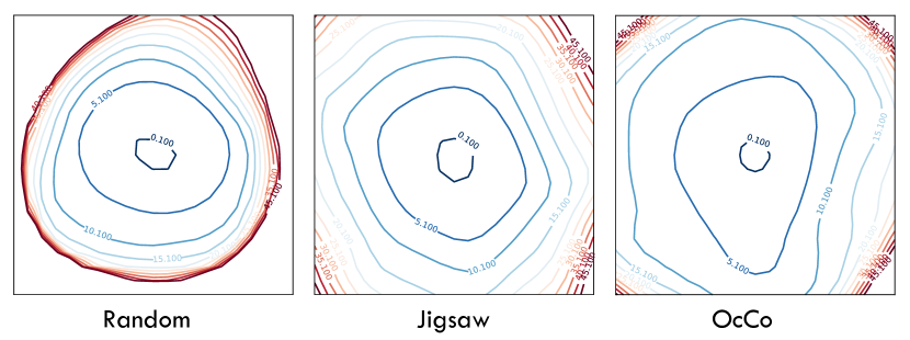
Figure 4: Loss landscape visualisation.

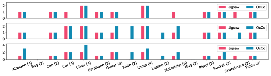
Figure 5: Number of detected object parts in the ‘Feat1’ (above), ‘Feat2’ (middle) and ‘Feat3’ (below) module of Jigsaw and OcCo-initialised PointNet feature encoder. Digits in the brackets are the number of parts under that object category.

Table 7: Adjusted mutual information (AMI) under transformations. We report the mean and standard error over 10 random initialisation. Under the ‘transformation’ column, ‘J’, ‘T’, ‘R’ represent jittering, translation and rotation, respectively.

Transformation			ShapeNet10				ScanObjectNN
J	T	R	VFH	M2DP	Jigsaw	OcCo	VFH	M2DP	Jigsaw	OcCo
			0.12$\pm$0.01	0.22$\pm$0.03	0.33$\pm$0.04	0.51$\pm$0.03	0.05$\pm$0.02	0.18$\pm$0.02	0.29$\pm$0.02	0.44$\pm$0.03
✓			0.12$\pm$0.02	0.19$\pm$0.02	0.32$\pm$0.02	0.45$\pm$0.02	0.06$\pm$0.02	0.17$\pm$0.02	0.27$\pm$0.02	0.42$\pm$0.04
✓	✓		0.13$\pm$0.03	0.21$\pm$0.02	0.29$\pm$0.07	0.38$\pm$0.04	0.04$\pm$0.02	0.18$\pm$0.03	0.24$\pm$0.04	0.39$\pm$0.06
✓	✓	✓	0.07$\pm$0.03	0.20$\pm$0.04	0.28$\pm$0.03	0.35$\pm$0.05	0.04$\pm$0.01	0.16$\pm$0.03	0.18$\pm$0.09	0.34$\pm$0.06

Visualisation of learned features.

We use feature visualisation to explore what a pre-trained model has learned about point cloud objects before fine-tuning. In Figure 3, we visualise the features/embeddings of the objects from the test split of ModelNet40. We colour the points according to their channel activations. The larger the activation value is, the darker the colour will be. We observe that the pre-trained encoder can learn low-level geometric primitives, e.g., planes, cylinders and cones, in the early stage. While it later recognises more complex shapes like wings, leaves and upper bodies. We further use t-SNE to visualise the object embeddings on ShapeNet10. We notice that distinguishable clusters are formed after pre-training. Thus, it seems that OcCo can learn features that are useful to distinguish different parts of an object or a scene. These features will be beneficial to downstream tasks, e.g., object classification and scene segmentation.

Unsupervised mutual information probe.

We hypothesise that a pre-trained model without fine-tuning can learn label information in an unsupervised fashion, i.e., zero-shot learning on cross-domain datasets. To validate, we utilise OcCo-PointNet to extract global features for objects from ShapeNet10 and ScanObjectNN. Then, we cluster the extracted embeddings with an unsupervised clustering method, K-means (where K is set to the number of object categories). To evaluate the clustering quality, we calculate the adjusted mutual information (AMI) [33] between the generated and the ground-truth clusters. AMI reaches 1 if two clusters are identical, while it has an expected value of 0 for a random categorical cluster assignment. Besides, we also study whether the OcCo-PointNet is robust to input transformations. In particular, we consider three transformations, including rotation, translation and jittering. We apply these transformations to an input point cloud before using PointNet for feature/embedding extraction.

We compare OcCo with Jigsaw and two hand-crafted point cloud global descriptors: viewpoint feature histogram (VFH) [40] and M2DP [17] in Table 7. We observe that pre-training methods, e.g., Jigsaw and OcCo , can learn more discriminative feature representations than hand-crafted descriptors, while the representations learned from OcCo pre-trained encoder are more predictive than Jigsaw based method. These results demonstrate that OcCo is effective for unsupervised feature learning.

Figure 6: Visualisation of detected concepts. Parts marked by blue and green are the binary masks based on the feature activations ($M_{k}$) and the ground truth labels ($C_{n}$).

Detection of semantic concepts.

We adapt network dissection [4, 5] to study whether OcCo pre-trained models can learn semantic concepts in an unsupervised fashion without fine-tuning. Specifically, for each object, we first create an activation mask $M_{k}$ based on the feature map from the $k$-th channel in the network. We assign the $i$-th entry of $M_{k}$ as 1 if the activation of the $i$-th point in that feature map is among the top 20%, otherwise the $i$-th entry is assigned to 0. The concept mask $C_{n}$ marks the points as 1 if they belong to the $n$-th semantic concept (e.g., chair legs) in the ground truth annotations. Given a set of point clouds $\mathcal{D}_{\mathcal{P}}$, we calculate the mean intersection of union (mIoU) scores based on these binary masks:

$$\text{mIoU}_{(k,n)}=\mathbb{E}_{\mathcal{P}\sim\mathcal{D}_{\mathcal{P}}}\left[\frac{\left|M_{k}(\mathcal{P})\cap C_{n}(\mathcal{P})\right|}{\left|M_{k}(\mathcal{P})\cup C_{n}(\mathcal{P})\right|}\right]$$ (13)

where $|\cdot|$ is the set cardinality. $\text{mIoU}_{(k,n)}$ can be interpreted as how well channel $k$ detects the concept $n$. In Figure 5, we plot the number of detected concepts (i.e., $\text{mIoU}_{(k,n)}>0.5$). We conclude that OcCo outperforms Jigsaw in terms of the total number of detected concepts. We visualise some masks from OcCo-PointNet in Figure 6. We observe that OcCo pre-training can capture rich concept information. These results demonstrate that pre-training with OcCo can unsupervisedly learn semantic concepts.

6 Discussion

In this work, we have demonstrated that Occlusion Completion (OcCo) can learn representations for point clouds that are accurate in few-shot learning, in object classification, and in part and semantic segmentation tasks, as compared to prior work. We performed multiple analyses to explain why this occurs, including a visualisation of the loss landscape, visualisation of learned features, tests of transformation invariance, and quantifying how well the initialisations can learn semantic concepts. In the future, it would be interesting to design a completion model that is explicitly aware of the occlusion procedure. This model would may converge even quicker and require fewer parameters, as this could act as a stronger inductive bias during learning.

7 Acknowledgements

We would like to thank Qingyong Hu, Shengyu Huang, Matthias Niessner, Kilian Q. Weinberger, and Trevor Darrell for valuable discussions and feedbacks.

Appendix A Implementation details

Completion pre-training

Previous point completion models [10, 60, 48, 51] all use an ”encoder-decoder” architecture. The encoder maps a partial point cloud to a vector of a fixed dimension, and the decoder reconstructs the full shape.

In the OcCo experiments, we exclude the last few MLPs of PointNet and DGCNN, and use the remaining architecture as the encoder to map a partial point cloud into a 1024-dimensional vector. We adapt the folding-based decoder design from PCN, which is a two-stage point cloud generator that generates a coarse and a fine-grained output point cloud $(Y_{coarse},Y_{fine})$ for each input feature. We sketch the network structures of PCN encoder and output layers for downstream tasks in Figure 7. We removed all the batch normalisation in the folding-based decoder since we find they bring negative effects in the completion process in terms of loss and convergence rate, this has been reported in image generations [34]. Also, we find L2 normalisation in the Adam optimiser is undesirable for completion training but brings improvements for the downstream fine-tuning tasks.

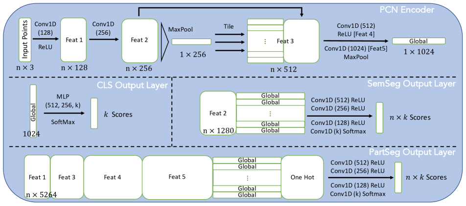
Figure 7: Encoder and Output Layers of PCN

We compare the occluded datasets based on ModelNet40 and ShapeNet8 for the OcCo pre-training. We construct the ModelNet Occluded using the methods described in Section 3 and for ShapeNet Occluded we directly use the data provided in the PCN, whose generation method are similar but not exactly the same with ours. Basic statistics of these two datasets are reported in Table 8.

Table 8: Statistics of occluded datasets for OcCo pre-training

Name	# of Class	# of Object	# of Views	# of Points/Object
ShapeNet Occluded (PCN and follow-ups)	8	30974	8	1045
ModelNet Occluded (OcCo )	40	12304	10	20085

By visualising the objects from the both datasets in Figure 8 and Figure 9, we show that our generated occluded shapes are more naturalistic and closer to real collected data. We believe this realism will be beneficial for the pre-training. We then test our hypothesis by pre-training models on one of the dataset, and fine tune them on the other. We report these results in Table 9. Clearly we see that the OcCo models pre-trained on ShapeNet Occluded do not perform as well as the ones pre-trained on ModelNet Occluded in most cases. Therefore we choose our generated ModelNet Occluded rather than ShapeNet Occlude [60, 48, 51] used in for the pre-training.

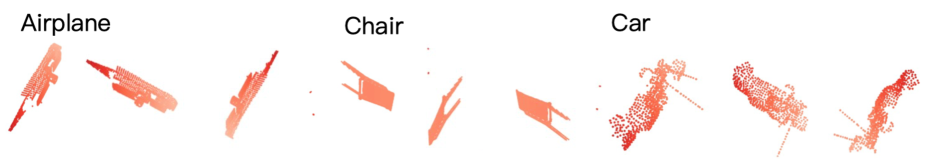
Figure 8: Examples from ShapeNet Occluded which fail to depict the underlying object shapes

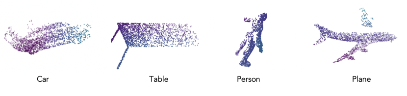
Figure 9: Examples of our generated self-occluded objects from ModelNet.

Table 9: Performance of OcCo pre-trained models with different pre-trained datasets

OcCo Settings		Classification Accuracy
Encoder	Pre-Trained Dataset	ModelNet Occ.	ShapeNet Occ.
PointNet	ShapeNet Occ.	81.0	94.1
	ModelNet Occ.	85.6	95.0
PCN	ShapeNet Occ.	81.6	94.4
	ModelNet Occ.	85.1	95.1
DGCNN	ShapeNet Occ.	86.7	94.5
	ModelNet Occ.	89.1	95.1

Re-Implementation details of ”Jigsaw” pre-training methods

We describe how we reproduce the ’Jigsaw’ pre-training methods from [42]. Following their description, we first separate the objects/chopped indoor scenes into $3^{3}=27$ small cubes and assign each point a label indicting which small cube it belongs to. We then shuffle all the small cubes, and train a model to make a prediction for each point. We reformulate this task as a 27-class semantic segmentation, for the details on the data generation and model training, please refer to our released code.

Appendix B Ablations

As pointed out by the reviewers, we agree adding more runs will help. To help judge significance, we have ran 10 runs for three settings and computed p-values via t-tests (unpaired, unequal variances) between OcCo and baselines (i.e., Jigsaw or random). We observe that all p-values are below the conventional significance threshold $\alpha\!=\!0.05$ (the family-wise error rate is also, using Holm-Bonferroni).

Table 10: P-values for unpaired (unequal variance) t-tests between OcCo and baselines (across 10 runs). Setting: (1) Few-Shot (10-way 10-shot), ScanObjectNN, DGCNN; (2) Classification, ScanNet, PCN; (3) Segmentation, SensatUrban, PointNet.

Setting	OcCo vs. Rand	OcCo vs. Jigsaw
(1)	$10^{-7}$	$10^{-7}$
(2)	$0.02$	$0.05$
(3)	$0.006$	$0.02$

As suggested by the reviewers, we ran ablations varying the number of object views and categories in Tables 11 and 12. We use Setting (1) from Table 10 as it is the fastest to run ($*$ indicates few-shot result in main paper).

Table 11: Ablation: number of views (5 runs), $*\!=\!$ main paper result.

# of Views	1	5	10*	20
PointNet	44.7$\pm$1.8	53.6$\pm$1.2	54.9$\pm$1.2	54.8$\pm$1.0
DGCNN	42.7$\pm$2.1	56.9$\pm$1.4	56.8$\pm$1.5	57.0$\pm$1.6

Table 12: Ablation: number of object categories (5 runs)

# of Categories	1	10	40*
PointNet	41.1$\pm$1.2	52.2$\pm$1.5	54.9$\pm$1.2
DGCNN	37.9$\pm$3.8	44.8$\pm$2.9	56.8$\pm$1.5

Appendix C More results

3D object classification with Linear SVMs

We follow the similar procedures from [1, 14, 42, 54, 59], to train a linear Support Vector Machine (SVM) to examine the generalisation of OcCo encoders that are pre-trained on the occluded objects from ModelNet40. For all six classification datasets, we fit a linear SVM on the output 1024-dimensional embeddings of the train split and evaluate it on the test split. Since [42] have already proven their methods are better than the prior, here we only systematically compare with theirs. We report the results in Table 13, we can see that all OcCo models achieve superior results compared to the randomly-initialised counterparts, demonstrating that OcCo pre-training helps the generalisation both in-domain and cross-domain.

Table 13: linear SVM on the output embeddings from random, Jigsaw and OcCo initialised encoders

Dataset	PointNet			PCN			DGCNN
	Rand	Jigsaw	OcCo	Rand	Jigsaw	OcCo	Rand	Jigsaw	OcCo
ShapeNet10	91.3	91.1	93.9	88.5	91.8	94.6	90.6	91.5	94.5
ModelNet40	70.6	87.5	88.7	60.9	73.1	88.0	66.0	84.9	89.2
ShapeNet Oc	79.1	86.1	91.1	72.0	87.9	90.5	78.3	87.8	91.6
ModelNet Oc	65.2	70.3	80.2	55.3	65.6	83.3	60.3	72.8	82.2
ScanNet10	64.8	64.1	67.7	62.3	66.3	75.5	61.2	69.4	71.2
ScanObjectNN	45.9	55.2	69.5	39.9	49.7	72.3	43.2	59.5	78.3

Few-shot learning

We use the same setting and train/test split as cTree [44], and report the mean and standard deviation across on 10 runs. The top half of the table reports results for eight randomly initialised point cloud models, while the bottom-half reports results on two models across three pre-training methods. We bold the best results (and those whose standard deviation overlaps the mean of the best result). It is worth mentioning cTree [44] pre-trained the encoders on both datasets before fine tuning, while we only pre-trained once on ModelNet40. The results show that models pre-trained with OcCo either outperform or have standard deviations that overlap with the best method in 7 out of 8 settings.

Table 14: More results on few-shot learning.

Baseline	ModelNet40				Sydney10
	5-way		10-way		5-way		10-way
	10-shot	20-shot	10-shot	20-shot	10-shot	20-shot	10-shot	20-shot
3D-GAN, Rand	55.8$\pm$10.7	65.8$\pm$9.9	40.3$\pm$6.5	48.4$\pm$5.6	54.2$\pm$4.6	58.8$\pm$5.8	36.0$\pm$6.2	45.3$\pm$7.9
FoldingNet, Rand	33.4 $\pm$13.1	35.8$\pm$18.2	18.6$\pm$6.5	15.4$\pm$6.8	58.9$\pm$5.6	71.2$\pm$6.0	42.6$\pm$3.4	63.5$\pm$3.9
Latent-GAN, Rand	41.6$\pm$16.9	46.2$\pm$19.7	32.9$\pm$9.2	25.5$\pm$9.9	64.5$\pm$6.6	79.8$\pm$3.4	50.5$\pm$3.0	62.5$\pm$5.1
PointCapsNet, Rand	42.3$\pm$17.4	53.0$\pm$18.7	38.0$\pm$14.3	27.2$\pm$14.9	59.4$\pm$6.3	70.5$\pm$4.8	44.1$\pm$2.0	60.3$\pm$4.9
PointNet++, Rand	38.5$\pm$16.0	42.4$\pm$14.2	23.1$\pm$7.0	18.8$\pm$5.4	79.9$\pm$6.8	85.0$\pm$5.3	55.4$\pm$2.2	63.4$\pm$2.8
PointCNN, Rand	65.4$\pm$8.9	68.6$\pm$7.0	46.6$\pm$4.8	50.0$\pm$7.2	75.8$\pm$7.7	83.4$\pm$4.4	56.3$\pm$2.4	73.1$\pm$4.1
PointNet, Rand	52.0$\pm$12.2	57.8$\pm$15.5	46.6$\pm$13.5	35.2$\pm$15.3	74.2$\pm$7.3	82.2$\pm$5.1	51.4$\pm$1.3	58.3$\pm$2.6
PointNet, cTree	63.2$\pm$10.7	68.9$\pm$9.4	49.2$\pm$6.1	50.1$\pm$5.0	76.5$\pm$6.3	83.7$\pm$4.0	55.5$\pm$2.3	64.0$\pm$2.4
PointNet, OcCo	89.7$\pm$6.1	92.4$\pm$4.9	83.9$\pm$5.6	89.7$\pm$4.6	77.7$\pm$8.0	84.9$\pm$4.9	60.9$\pm$3.7	65.5$\pm$5.5
DGCNN, Rand	31.6 $\pm$9.0	40.8$\pm$14.6	19.9$\pm$6.5	16.9$\pm$4.8	58.3$\pm$6.6	76.7$\pm$7.5	48.1$\pm$8.2	76.1$\pm$3.6
DGCNN, cTree	60.0$\pm$8.9	65.7$\pm$8.4	48.5$\pm$5.6	53.0$\pm$4.1	86.2$\pm$4.4	90.9$\pm$2.5	66.2$\pm$2.8	81.5$\pm$2.3
DGCNN, OcCo	90.6$\pm$2.8	92.5$\pm$6.0	82.9$\pm$4.1	86.5$\pm$7.1	79.9$\pm$6.7	86.4$\pm$4.7	63.3$\pm$2.7	77.6$\pm$3.9

Detailed results of the part segmentation

Here in Table 15 we report the detailed scores on each individual shape category from ShapeNetPart, we bold the best scores for each class respectively. We show that for all three encoders, OcCo-initialisation has achieved better results over two thirds of these 15 object classes.

Table 15: Detailed Results on Part Segmentation Task on ShapeNetPart

Shapes	PointNet			PCN			DGCNN
	Rand*	Jigsaw	OcCo	Rand	Jigsaw	OcCo	Rand*	Jigsaw*	OcCo
mean (point)	83.7	83.8	84.4	82.8	82.8	83.7	85.1	85.3	85.5
Aero	83.4	83.0	82.9	81.5	82.1	82.4	84.2	84.1	84.4
Bag	78.7	79.5	77.2	72.3	74.2	79.4	83.7	84.0	77.5
Cap	82.5	82.4	81.7	85.5	67.8	86.3	84.4	85.8	83.4
Car	74.9	76.2	75.6	71.8	71.3	73.9	77.1	77.0	77.9
Chair	89.6	90.0	90.0	88.6	88.6	90.0	90.9	90.9	91.0
Earphone	73.0	69.7	74.8	69.2	69.1	68.8	78.5	80.0	75.2
Guitar	91.5	91.1	90.7	90.0	89.9	90.7	91.5	91.5	91.6
Knife	85.9	86.3	88.0	84.0	83.8	85.9	87.3	87.0	88.2
Lamp	80.8	80.7	81.3	78.5	78.8	80.4	82.9	83.2	83.5
Laptop	95.3	95.3	95.4	95.3	95.1	95.6	96.0	95.8	96.1
Motor	65.2	63.7	65.7	64.1	64.7	64.2	67.8	71.6	65.5
Mug	93.0	92.3	91.6	90.3	90.8	92.6	93.3	94.0	94.4
Pistol	81.2	80.8	81.0	81.0	81.5	81.5	82.6	82.6	79.6
Rocket	57.9	56.9	58.2	51.8	51.4	53.8	59.7	60.0	58.0
Skateboard	72.8	75.9	74.2	72.5	71.0	73.2	75.5	77.9	76.2
Table	80.6	80.8	81.8	81.4	81.2	81.2	82.0	81.8	82.8

Appendix D Algorithmic Description of OcCo

Algorithm 1 Occlusion Completion (OcCo)

⬇ # P: an initial point cloud # K: camera intrinsic matrix # V: number of total view points # loss: a loss function between point clouds # c: encoder-decoder completion model # p: downstream prediction model while i < V: # sample a random view-point R_t = [random.rotation(), random.translation()] # map point cloud to camera reference frame P_cam = dot(K, dot(R_t, P)) # create occluded point cloud P_cam_oc = occlude(P_cam, alg=’z-buffering’) # point cloud back to world frame K_inv = [inv(K), zeros(3,1); zeros(1,3), 1] R_t_inv = transpose([R_t; zeros(3,1), 1]) P_oc = dot(R_t_inv, dot(K_inv, P_cam_oc)) # complete point cloud P_c = c.decoder(c.encoder(P_oc)) # compute loss, update via gradient descent l = loss(P_c, P) l.backward() update(c.params) i += 1 # downstream tasks, use pre-trained encoders p.initialise(c.encoder.params) p.train()

Appendix E Visualisation from Completion Pre-Training

In this section, we show some qualitative results of OcCo pre-training by visualising the input, coarse output, fine output and ground truth at different training epochs and encoders. In Figure. 10, Figure. 11 and Figure. 12, we notice that the trained completion models are able to complete even difficult occluded shapes such as plants and planes. In Figure. 13 we plot some failure examples of completed shapes, possibly due to their complicated fine structures, while it is worth mentioning that the completed model can still completed these objects under the same category.

Figure 10: OcCo pre-training with PCN encoder on occluded ModelNet40.

Figure 11: OcCo pre-training with PointNet encoder on occluded ModelNet40.

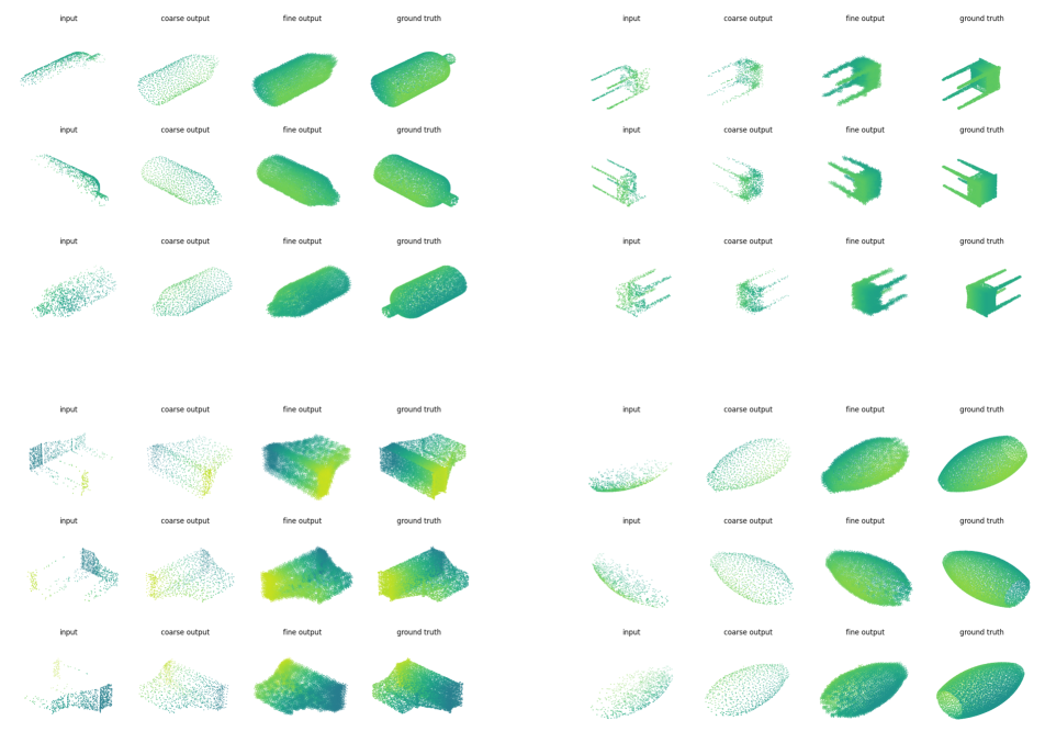
Figure 12: OcCo pre-training with DGCNN encoder on occluded ModelNet40.

Figure 13: Failure completed examples during OcCo pre-training.

References

- [1] Panos Achlioptas, Olga Diamanti, Ioannis Mitliagkas, and Leonidas J. Guibas. Learning representations and generative models for 3d point clouds. In International Conference on Machine Learning, (ICML), 2018.
- [2] Antonio Alliegro, Davide Boscaini, and Tatiana Tommasi. Joint supervised and self-supervised learning for 3d real-world challenges. arXiv preprint arXiv:2004.07392, 2020.
- [3] Iro Armeni, Ozan Sener, Amir R Zamir, Helen Jiang, Ioannis Brilakis, Martin Fischer, and Silvio Savarese. 3d semantic parsing of large-scale indoor spaces. In The IEEE Conference on Computer Vision and Pattern Recognition (CVPR), 2016.
- [4] David Bau, Bolei Zhou, Aditya Khosla, Aude Oliva, and Antonio Torralba. Network dissection: Quantifying interpretability of deep visual representations. In The IEEE Conference on Computer Vision and Pattern Recognition (CVPR), 2017.
- [5] David Bau, Jun-Yan Zhu, Hendrik Strobelt, Agata Lapedriza, Bolei Zhou, and Antonio Torralba. Understanding the role of individual units in a deep neural network. Proceedings of the National Academy of Sciences, 2020.
- [6] Alina Beygelzimer, Sham Kakade, and John Langford. Cover trees for nearest neighbor. In Proceedings of the 23rd international conference on Machine learning (ICML), 2006.
- [7] Pratik Chaudhari, Anna Choromanska, Stefano Soatto, Yann LeCun, Carlo Baldassi, Christian Borgs, Jennifer T. Chayes, Levent Sagun, and Riccardo Zecchina. Entropy-sgd: Biasing gradient descent into wide valleys. In International Conference on Learning Representations (ICLR), 2017.
- [8] Ting Chen, Simon Kornblith, Mohammad Norouzi, and Geoffrey Hinton. A simple framework for contrastive learning of visual representations. International Conference on Machine Learning (ICML), 2020.
- [9] Angela Dai, Christian Diller, and Matthias Nießner. Sg-nn: Sparse generative neural networks for self-supervised scene completion of rgb-d scans. In Proceedings of the IEEE/CVF Conference on Computer Vision and Pattern Recognition (CVPR), 2020.
- [10] Angela Dai, Charles Ruizhongtai Qi, and Matthias Nießner. Shape completion using 3d-encoder-predictor cnns and shape synthesis. In The IEEE Conference on Computer Vision and Pattern Recognition (CVPR), 2017.
- [11] Jacob Devlin, Ming-Wei Chang, Kenton Lee, and Kristina Toutanova. Bert: Pre-training of deep bidirectional transformers for language understanding. arXiv preprint arXiv:1810.04805, 2018.
- [12] Matheus Gadelha, Aruni RoyChowdhury, Gopal Sharma, Evangelos Kalogerakis, Liangliang Cao, Erik Learned-Miller, Rui Wang, and Subhransu Maji. Label-efficient learning on point clouds using approximate convex decompositions. In European conference on computer vision (ECCV), 2020.
- [13] Timo Hackel, N. Savinov, L. Ladicky, Jan D. Wegner, K. Schindler, and M. Pollefeys. SEMANTIC3D.NET: A new large-scale point cloud classification benchmark. In ISPRS Annals of the Photogrammetry, Remote Sensing and Spatial Information Sciences, volume IV-1-W1, pages 91–98, 2017.
- [14] Zhizhong Han, Mingyang Shang, Yu-Shen Liu, and Matthias Zwicker. View inter-prediction gan: Unsupervised representation learning for 3d shapes by learning global shape memories to support local view predictions. In Proceedings of the AAAI Conference on Artificial Intelligence, 2019.
- [15] Kaveh Hassani and Mike Haley. Unsupervised multi-task feature learning on point clouds. In The IEEE International Conference on Computer Vision (CVPR), 2019.
- [16] Kaiming He, Haoqi Fan, Yuxin Wu, Saining Xie, and Ross Girshick. Momentum contrast for unsupervised visual representation learning. The IEEE Conference on Computer Vision and Pattern Recognition (CVPR), 2020.
- [17] Li He, Xiaolong Wang, and Hong Zhang. M2dp: A novel 3d point cloud descriptor and its application in loop closure detection. In IEEE/RSJ International Conference on Intelligent Robots and Systems (IROS), 2016.
- [18] Sepp Hochreiter and Jürgen Schmidhuber. Flat minima. Neural computation, 9(1):1–42, 1997.
- [19] Ji Hou, Angela Dai, and Matthias Nießner. Revealnet: Seeing behind objects in rgb-d scans. In Proceedings of the IEEE/CVF Conference on Computer Vision and Pattern Recognition (CVPR), 2020.
- [20] Ji Hou, Benjamin Graham, Matthias Nießner, and Saining Xie. Exploring data-efficient 3d scene understanding with contrastive scene contexts. arXiv preprint arXiv:2012.09165, 2020.
- [21] Qingyong Hu, Bo Yang, Sheikh Khalid, Wen Xiao, Niki Trigoni, and Andrew Markham. Towards semantic segmentation of urban-scale 3d point clouds: A dataset, benchmarks and challenges. arXiv preprint arXiv:2009.03137, 2020.
- [22] Qingyong Hu, Bo Yang, Linhai Xie, Stefano Rosa, Yulan Guo, Zhihua Wang, Niki Trigoni, and Andrew Markham. Randla-net: Efficient semantic segmentation of large-scale point clouds. Proceedings of the IEEE Conference on Computer Vision and Pattern Recognition (CVPR), 2020.
- [23] Weihua Hu, Bowen Liu, Joseph Gomes, Marinka Zitnik, Percy Liang, Vijay Pande, and Jure Leskovec. Strategies for pre-training graph neural networks. In International Conference on Learning Representations (ICLR), 2020.
- [24] Ziniu Hu, Yuxiao Dong, Kuansan Wang, Kai-Wei Chang, and Yizhou Sun. Gpt-gnn: Generative pre-training of graph neural networks. In Proceedings of the 26th ACM SIGKDD International Conference on Knowledge Discovery and Data Mining (KDD), 2020.
- [25] Diederik P. Kingma and Jimmy Ba. Adam: A method for stochastic optimization. In International Conference on Learning Representations (ICLR), 2015.
- [26] Loic Landrieu and Martin Simonovsky. Large-scale point cloud semantic segmentation with superpoint graphs. In The IEEE Conference on Computer Vision and Pattern Recognition (CVPR), 2018.
- [27] Alex H Lang, Sourabh Vora, Holger Caesar, Lubing Zhou, Jiong Yang, and Oscar Beijbom. Pointpillars: Fast encoders for object detection from point clouds. In The IEEE Conference on Computer Vision and Pattern Recognition (CVPR), 2019.
- [28] Hao Li, Zheng Xu, Gavin Taylor, Christoph Studer, and Tom Goldstein. Visualizing the loss landscape of neural nets. In Advances in Neural Information Processing Systems (NeurIPS), 2018.
- [29] Jiaxin Li, Ben M Chen, and Gim Hee Lee. So-net: Self-organizing network for point cloud analysis. In The IEEE conference on computer vision and pattern recognition (CVPR), 2018.
- [30] Yangyan Li, Rui Bu, Mingchao Sun, and Baoquan Chen. Pointcnn. Advances in neural information processing systems (NeurIPS), 2018.
- [31] Ilya Loshchilov and Frank Hutter. SGDR: stochastic gradient descent with warm restarts. In International Conference on Learning Representations, (ICLR), 2017.
- [32] Tomas Mikolov, Kai Chen, Greg Corrado, and Jeffrey Dean. Efficient estimation of word representations in vector space. arXiv preprint arXiv:1301.3781, 2013.
- [33] Xuan Vinh Nguyen, Julien Epps, and James Bailey. Information theoretic measures for clusterings comparison: is a correction for chance necessary? In International Conference on Machine Learning (ICML), 2009.
- [34] Taesung Park, Ming-Yu Liu, Ting-Chun Wang, and Jun-Yan Zhu. Semantic image synthesis with spatially-adaptive normalization. In Proceedings of the IEEE/CVF Conference on Computer Vision and Pattern Recognition, pages 2337–2346, 2019.
- [35] Deepak Pathak, Philipp Krahenbuhl, Jeff Donahue, Trevor Darrell, and Alexei A Efros. Context encoders: Feature learning by inpainting. In Proceedings of the IEEE conference on computer vision and pattern recognition (CVPR), 2016.
- [36] Matthew E. Peters, Mark Neumann, Mohit Iyyer, Matt Gardner, Christopher Clark, Kenton Lee, and Luke Zettlemoyer. Deep contextualized word representations. In The North American Chapter of the Association for Computational Linguistics: Human Language Technologies, (NAACL-HLT), 2018.
- [37] Charles R Qi, Hao Su, Kaichun Mo, and Leonidas J Guibas. Pointnet: Deep learning on point sets for 3d classification and segmentation. In The IEEE conference on computer vision and pattern recognition (CVPR), 2017.
- [38] Charles Ruizhongtai Qi, Li Yi, Hao Su, and Leonidas J Guibas. Pointnet++: Deep hierarchical feature learning on point sets in a metric space. In Advances in neural information processing systems (NeurIPS), 2017.
- [39] Can Qin, Haoxuan You, Lichen Wang, C.-C. Jay Kuo, and Yun Fu. Pointdan: A multi-scale 3d domain adaption network for point cloud representation. In Advances in Neural Information Processing Systems (NeurIPS), 2019.
- [40] Radu Bogdan Rusu, Gary Bradski, Romain Thibaux, and John Hsu. Fast 3d recognition and pose using the viewpoint feature histogram. In IEEE/RSJ International Conference on Intelligent Robots and Systems (IROS), 2010.
- [41] Radu Bogdan Rusu and Steve Cousins. 3D is here: Point Cloud Library (PCL). In The IEEE International Conference on Robotics and Automation (ICRA), 2011.
- [42] Jonathan Sauder and Bjarne Sievers. Self-supervised deep learning on point clouds by reconstructing space. In Advances in Neural Information Processing Systems (NeurIPS), 2019.
- [43] Johannes L Schönberger, Marc Pollefeys, Andreas Geiger, and Torsten Sattler. Semantic visual localization. In Proceedings of the IEEE Conference on Computer Vision and Pattern Recognition (CVPR), 2018.
- [44] Charu Sharma and Manohar Kaul. Self-supervised few-shot learning on point clouds. In Advances in Neural Information Processing Systems (NeurIPS), 2020.
- [45] Shuran Song, Fisher Yu, Andy Zeng, Angel X Chang, Manolis Savva, and Thomas Funkhouser. Semantic scene completion from a single depth image. In Proceedings of the IEEE Conference on Computer Vision and Pattern Recognition (CVPR), 2017.
- [46] Nitish Srivastava, Geoffrey Hinton, Alex Krizhevsky, Ilya Sutskever, and Ruslan Salakhutdinov. Dropout: A simple way to prevent neural networks from overfitting. Journal of Machine Learning Research, 15(56):1929–1958, 2014.
- [47] Wolfgang Straßer. Schnelle kurven-und flächendarstellung auf grafischen sichtgeräten. PhD thesis, 1974.
- [48] Lyne P. Tchapmi, Vineet Kosaraju, Hamid Rezatofighi, Ian Reid, and Silvio Savarese. Topnet: Structural point cloud decoder. In The IEEE Conference on Computer Vision and Pattern Recognition (CVPR), 2019.
- [49] Mikaela Angelina Uy, Quang-Hieu Pham, Binh-Son Hua, Thanh Nguyen, and Sai-Kit Yeung. Revisiting point cloud classification: A new benchmark dataset and classification model on real-world data. In IEEE International Conference on Computer Vision (ICCV), 2019.
- [50] Bernie Wang, Virginia Wu, Bichen Wu, and Kurt Keutzer. Latte: accelerating lidar point cloud annotation via sensor fusion, one-click annotation, and tracking. In The IEEE Intelligent Transportation Systems Conference (ITSC), 2019.
- [51] Xiaogang Wang, Marcelo H. Ang, and Gim Hee Lee. Cascaded refinement network for point cloud completion. In The IEEE Conference on Computer Vision and Pattern Recognition (CVPR), 2020.
- [52] Yue Wang, Alireza Fathi, Abhijit Kundu, David Ross, Caroline Pantofaru, Tom Funkhouser, and Justin Solomon. Pillar-based object detection for autonomous driving. In European Conference on Computer Vision (ECCV), 2020.
- [53] Yue Wang, Yongbin Sun, Ziwei Liu, Sanjay E Sarma, Michael M Bronstein, and Justin M Solomon. Dynamic graph cnn for learning on point clouds. ACM Transactions on Graphics (TOG), 38(5):1–12, 2019.
- [54] Jiajun Wu, Chengkai Zhang, Tianfan Xue, Bill Freeman, and Josh Tenenbaum. Learning a probabilistic latent space of object shapes via 3d generative-adversarial modeling. In Advances in neural information processing systems (NeurIPS), 2016.
- [55] Zhirong Wu, Shuran Song, Aditya Khosla, Fisher Yu, Linguang Zhang, Xiaoou Tang, and Jianxiong Xiao. 3d shapenets: A deep representation for volumetric shapes. In the IEEE conference on computer vision and pattern recognition (CVPR), 2015.
- [56] Saining Xie, Jiatao Gu, Demi Guo, Charles R Qi, Leonidas J Guibas, and Or Litany. Pointcontrast: Unsupervised pre-training for 3d point cloud understanding. In European conference on computer vision (ECCV), 2020.
- [57] Bo Yang, Jianan Wang, Ronald Clark, Qingyong Hu, Sen Wang, Andrew Markham, and Niki Trigoni. Learning object bounding boxes for 3d instance segmentation on point clouds. In Advances in Neural Information Processing Systems (NeurIPS), 2019.
- [58] Guandao Yang, Xun Huang, Zekun Hao, Ming-Yu Liu, Serge Belongie, and Bharath Hariharan. Pointflow: 3d point cloud generation with continuous normalizing flows. In Proceedings of the IEEE/CVF Conference on Computer Vision and Pattern Recognition (CVPR), 2019.
- [59] Yaoqing Yang, Chen Feng, Yiru Shen, and Dong Tian. Foldingnet: Point cloud auto-encoder via deep grid deformation. In Proceedings of the IEEE Conference on Computer Vision and Pattern Recognition, pages 206–215, 2018.
- [60] Wentao Yuan, Tejas Khot, David Held, Christoph Mertz, and Martial Hebert. Pcn: Point completion network. In 2018 International Conference on 3D Vision (3DV), pages 728–737. IEEE, 2018.
- [61] Zaiwei Zhang, Rohit Girdhar, Armand Joulin, and Ishan Misra. Self-supervised pretraining of 3d features on any point-cloud. arXiv:2101.02691, 2021.
- [62] Yongheng Zhao, Tolga Birdal, Haowen Deng, and Federico Tombari. 3d point capsule networks. In Proceedings of the IEEE Conference on Computer Vision and Pattern Recognition (CVPR), 2019.
- [63] Qian-Yi Zhou and Ulrich Neumann. Complete residential urban area reconstruction from dense aerial lidar point clouds. Graphical Models, 75(3):118–125, 2013.
- [64] Yin Zhou and Oncel Tuzel. Voxelnet: End-to-end learning for point cloud based 3d object detection. In The IEEE Conference on Computer Vision and Pattern Recognition (CVPR), 2018.
- [65] Xinge Zhu, Hui Zhou, Tai Wang, Fangzhou Hong, Yuexin Ma, Wei Li, Hongsheng Li, and Dahua Lin. Cylindrical and asymmetrical 3d convolution networks for lidar segmentation. arXiv preprint arXiv:2011.10033, 2020.
- [66] SM Zolanvari, Susana Ruano, Aakanksha Rana, Alan Cummins, Rogerio Eduardo da Silva, Morteza Rahbar, and Aljosa Smolic. Dublincity: Annotated lidar point cloud and its applications. In British Machine Vision Conference (BMVC), 2019.