DC power grids with constant-power loads—Part I: A full characterization of power flow feasibility, long-term voltage stability and their correspondence

Abstract

In this two-part paper we develop a unifying framework for the analysis of the feasibility of the power flow equations for DC power grids with constant-power loads.

In Part I of this paper we present a detailed introduction to the problem of power flow feasibility of such power grids, and the associated problem of selecting a desirable operating point which satisfies the power flow equations. We introduce and identify all long-term voltage semi-stable operating points, and show that there exists a one-to-one correspondence between such operating points and the constant power demands for which the power flow equations are feasible. Such operating points can be found by solving an initial value problem, and a parametrization of these operating points is also obtained. In addition, we give a full characterization of the set of all feasible power demands, and give a novel proof for the convexity of this set. Moreover, we present a necessary and sufficient LMI condition for the feasibility of a vector of power demands under small perturbation, which extends a necessary condition in the literature.

I Introduction

A classical problem in the study of power grid stability is the long-term voltage stability problem. The problem concerns the long-term (in)stability of a power grid due to limitations in the transportation of power from sources to loads. These limits in power transportation are due to a combination of generation limits, load limits and/or limits due to the network (infra)structure. The transportation of power from sources to loads is known as power flow or load flow, and is captured in the power flow equations (or also, load flow equations). Consequently, the power flow equations implicitly describe the limitations of power flow in a power grid.

Another motivation for the study of power flow are phenomena such as voltage drop, voltage collapse and power outages. Such phenomena may occur when transportation limits are exceeded and the power flow equations cannot be satisfied. Loosely speaking, control schemes which are designed to satisfy the power flow equations in the long-term time scale may display unintended behavior when the the power flow equations cannot be satisfied. A possible consequence is that critical components may reach their operational limits, start to fail, and cause a chain reaction of more failures. Satisfaction of the power flow equations is therefore crucial to guarantee (long-term) safe operation of the power grid.

Long-term voltage instability is a load-driven phenomenon [1], and different load characteristics may be considered for analysis—see, e.g., [2]. For a load characteristic with given parameters, we refer to solutions of the power flow equations as operating points of the power grid. The power flow equations are feasible if at least one operating point exists. In general, the power flow equations are nonlinear, and no operating points may exist. Likewise, multiple operating points may exist, while a single operating point should be selected.

For practical power grids there are several distinct properties to select an operating point. First, it is desirable that an operating point is long-term voltage stable, meaning that all voltage magnitudes of an operating point decrease if any load demand increases [1]. This is to say that the Jacobian of the voltage magnitudes at the loads as a function of the power demand has negative elements [3]. Second, it is desirable that the selected operating point is the solution to the power flow equations that minimizes the total power dissipated in the lines at steady state. A third property is that the operating point is a high-voltage solution, meaning that the selected operating point element-wise dominates all other operating point that satisfy the power flow equation.

It is a priori not clear if, or under which conditions, these types of operating points coincide, or give rise to a unique operating point. For specific types of power grids it has been shown that these types of operating point coincide “almost surely”, and that a sufficient condition exists for the uniqueness of the long-term voltage stable operating point [4]. A similar result for a general power grid is not available in the literature, but several sufficient conditions for are known [5, 3, 6].

There have been several publications on the problem of long-term voltage stability, and in particular on the feasibility of power flow equations. Here we list a few of them.
The paper [6] considers a generic AC power grid with a single source, whereas the paper [3] considers a lossless AC power grid. Both [3] and [6] give a sufficient condition for feasibility of the reactive power flow equations, and use fixed-point methods to conclude the existence of an operating point. Estimates of the operating point are also given. In addition, [3] shows that this operating point is the high-voltage solution, and that it is long-term voltage stable.
The paper [7] considers a general power transportation system at steady state and proves a necessary conditions for feasibility of a power demand, which is also sufficient in certain cases.
The paper [4] presents an algorithm to determine if the power flow equations of a DC power grid are feasible, and shows that there exists a high-voltage solution, which is “almost surely” long-term voltage stable. Conditions for the long-term voltage stable operating point to be unique are given.
The paper [8] proves that the set of feasible solutions to the power flow equations for DC power grids is convex, as follows from the study of convexity of the non-homogeneous numerical range of a generalized quadratic form.

In this two-part paper we focus on the power flow of DC power grids with constant-power loads, and assume there are no limits on voltage potentials and line currents. While many types of power grids are studied in the literature, DC power grids with constant-power loads are among the simplest type of power grid where feasibility of the power flow equations is nontrivial.

It is noted that there are several types of power grids for which the power flow equations are equivalent to or well-approximated by the power flow of DC power grids with constant-power loads. The paper [9] shows how the active power flow problem for a lossless AC power grid may be approximated by a DC power flow grid. The papers [10, 3] show a similar result for the reactive power flow problem for a lossless AC power grid. See also [6, 4] for other examples.

Even though the literature provides handles to study power flow, the interplay between the different results is not clear, and an over-arching analysis is missing. The main motivation of this paper is to bridge these gaps in the literature for DC power grids, and to develop a unified framework for the analysis of DC power flow with constant-power loads.

Contribution

This paper is split into two parts. Part I of this paper presents a geometric framework to analyze the feasibility of the DC power flow equations with constant-power loads. This framework is extended in Part II to unify and generalize the main contributions of the previously mentioned publications in the context of DC power flow. The novelty of our approach is that we combine results in matrix theory, convex analysis, and initial value problems to analyze DC power flow. In contrast to other approaches, we do not explicitly rely on fixed point analysis or iterative methods.

The main objective of this twin paper is to analyze the set, denoted by $\mathcal{F}$, of constant power demands for which the power flow equations are feasible. We would like to emphasize that these constant power demands are not sign-restricted. I.e., the power demand at a load is allowed to be negative, in which case the load provides power to the grid. We let $\mathcal{D}$ denote the set of long-term voltage stable operating points. We refer to the vectors in $\operatorname{cl}(\mathcal{D})$, the closure of $\mathcal{D}$, as long-term voltage semi-stable operating points.

In Part I of this paper we develop a geometric framework for DC power flow feasibility for constant-power loads. The main contributions of Part I are as follows.

1. We give a parametrization of $\mathcal{D}$, its closure and its boundary, which establishes a constructive method to describe the long-term voltage (semi-)stable operating points (Theorem III.7).

2. For each vector of power demand that lies on the boundary of $\mathcal{F}$ there exists a unique corresponding operating point which solves the power flow equations. Moveover, these operating points form the boundary of $\mathcal{D}$ (Corollary III.20).

3. There is a one-to-one correspondence between the feasible power demands $\mathcal{F}$ and the long-term voltage semi-stable operating points $\operatorname{cl}(\mathcal{D})$. This means that if the power flow equations are feasible, then there exists a unique long-term voltage semi-stable operating point that solves the power flow equations. This operating point can be found by solving an initial value problem (Theorem III.17).

4. We give a novel and insightful proof for the fact that the set $\mathcal{F}$ is closed and convex. Consequently, $\mathcal{F}$ is the intersection of all supporting half-spaces of $\mathcal{F}$. We describe all such half-spaces, which gives a complete geometric characterization of $\mathcal{F}$ (Theorem III.18).

5. We prove a necessary and sufficient LMI condition for the feasibility of the power flow equations, and a necessary and sufficient LMI condition for the feasibility of the power flow equations under small perturbations of the power demands (Theorem III.22).

Part II of this paper continues the approach, and recovers and extends several results of the previously mentioned publications for DC power grids with constant-power loads. The main contributions of Part II are as follows.

1. We give an alternative parametrization of $\mathcal{D}$, its closure and its boundary.

2. We give two parametrizations of $\partial\mathcal{F}$, the boundary of the set of feasible power demands.

3. We refine the results of M7 and M5 for nonnegative power demands, which are cheaper to compute.

4. We prove that any vector of power demands that is element-wise dominated by a feasible vector of power demands is also feasible.

5. We present two novel sufficient conditions for the feasibility of the power flow equations which generalize the sufficient conditions in [3] and [6], and show how these conditions are related.

6. We show that the long-term voltage stable operating point is a strict high-voltage solution. Consequently, the operating points associated to a feasible power demand which are either long-term voltage stable, a high-voltage solution, or dissipation-minimizing, are one and the same.

It is important to explain how these results are related to the existing literature, and in which regard these results are, to the best of the authors’ knowledge, novel.

Regarding M3, it was shown in [4] that if the power flow equations are feasible, then there “almost surely” exists an operating point which is long-term voltage stable, and that it is the unique long-term voltage stable operating point if all power demands are positive, or all are negative. By studying long-term voltage semi-stable operating points, we show that for each feasible vector of power demands there always exists a unique long-term semi-stable operating point.
Regarding M4, the convexity of $\mathcal{F}$ was already shown in [8] (see also [11]), and follows from an analysis of the convexity of the numerical range of non-homogeneous quadratic maps. Our approach to prove convexity is different from and less general than the one proposed by [8], and is a byproduct of the proof of M3, the one-to-one correspondence between $\mathcal{F}$ and $\operatorname{cl}(\mathcal{D})$. We believe our proof for convexity to be simpler.
Regarding M5, our contribution is a necessary and sufficient condition for the feasibility of power demands under small perturbations. In [7] a similar condition was shown to be sufficient for a more general system with constant-power loads at steady-state. It was shown in [7] to also be necessary whenever $\mathcal{F}$ is closed convex, as is the case here.
Regarding M11, it was shown in [4] that, if the power flow equations are feasible, then there exists a high-voltage solution, i.e., an operating point that element-wise dominates all other operating points which satisfy the power flow equations, and that this operating point is “almost surely” long-term voltage stable. We show that the element-wise domination is strict, and that this operating point always coincides with the unique long-term voltage semi-stable operating point. This shows the algorithm proposed in [4] converges to the unique long-term voltage semi-stable operating point wherever the power flow equations are feasible.

Organization of Part I

In Section II we formulate the DC power flow equations, discuss the problem of their feasibility, and define different types of desirable operating points. We give a detailed introduction to this feasibility problem and its difficulties.

In Section III we develop a geometric framework to analyze the DC power flow equations. The main objective of Section III is to prove that there is a one-to-one correspondence between $\mathcal{F}$ and $\mathcal{D}$, and to give a method to compute the desired operating point (M3). In addition, we prove that $\mathcal{F}$ is convex and present a full geometric characterization of $\mathcal{F}$ as an intersection of half-spaces (M4). To establish this, we present a parametrization of $\mathcal{D}$ (M1), and prove that there is a one-to-one correspondence between the boundary of $\mathcal{D}$ and the boundary of the convex hull of $\mathcal{F}$, which is a prelude to proving that there is a one-to-one correspondence between the boundary of $\mathcal{D}$ and the boundary of $\mathcal{F}$ (M2). The section is concluded by presenting a necessary and sufficient LMI condition for the feasibility of a vector of power demands, and a similar condition for feasibility under small perturbation (M5).

Section IV concludes Part I of the paper.

Notation and matrix definitions

For a vector $x=\begin{pmatrix}x_{1}&\cdots&x_{k}\end{pmatrix}^{\top}$ we denote

$$[x]:=\operatorname{diag}(x_{1},\dots,x_{k}).$$

We let $\mbb{1}$ and $\mbb{0}$ denote the all-ones and all-zeros vector, respectively, and let $I$ denote the identity matrix. We let their dimensions follow from their context. All vector and matrix inequalities are taken to be element-wise. We write $x\lneqq y$ if $x\leq y$ and $x\neq y$. We let $\|x\|_{p}$ denote the $p$-norm of $x\in\mathbb{R}^{k}$.

We define $\boldsymbol{n}:=\{1,\dots,n\}$. All matrices are square $n\times n$ matrices, unless stated otherwise. The submatrix of a matrix $A$ with rows and columns indexed by $\alpha,\beta\subseteq\boldsymbol{n}$, respectively, is denoted by $A_{[\alpha,\beta]}$. The same notation $v_{[\alpha]}$ is used for subvectors of a vector $v$. We let $\alpha^{\mathrm{c}}$ denote the set-theoretic complement of $\alpha$ with respect to $\boldsymbol{n}$. For a set $S$, the notation $\operatorname{int}(S)$, $\operatorname{cl}(S)$, $\partial S$ and $\operatorname{conv}(S)$ is used for the interior, closure, boundary and convex hull of $S$, respectively.

We list some classical definitions from matrix theory.

Definition I.1 ([12], Ch. 5)

A matrix $A$ is a Z-matrix if $A_{ij}\leq 0$ for all $i\neq j$.

Definition I.2 ([12], Thm. 5.3)

A Z-matrix is an M-matrix if all its eigenvalues have nonnegative real part.

Definition I.3 ([12], pp. 71)

A matrix $A$ is irreducible if for every nonempty set $\alpha\subsetneqq\boldsymbol{n}$ we have $A_{[\alpha,\alpha^{\mathrm{c}}]}\neq 0$.

II The DC power flow problem

In this section we formulate the DC power flow equations and explore their feasibility.

We study DC power grids that consist of nodes (buses), which are either loads or sources, and are interconnected by lines. Source nodes are voltage controlled buses which provide power to the power grid, and represent generators such as power plants. Load nodes are voltage controlled buses which generically extract power from the power grid. The power flow equations describe the power balance at the load nodes. We are interested in the existence of a solution to the power flow equations in the long-term time scale, and therefore study DC power grid at steady-state. Note that, at steady-state, the line dynamics do not contribute to this power balance. We therefore model the power grid as a resistive circuit. We refer to [13, 14] for a detailed discussion on resistive circuits.

We proceed with the modeling of DC power grids with purely resistive lines at steady state. For the sake of simpli- city we do not consider operational limits on lines, currents or voltage potentials in the power grid. We consider a DC power grid with $n$ load nodes and $m$ source nodes. We write $i\sim j$ if there exists a line between node $i$ and node $j$, and $i\not\sim j$ otherwise. The conductance of the line between node $i$ and node $j$ is denoted by $w_{ij}=w_{ji}$, which is a positive real number. The Kirchhoff matrix $Y\in\mathbb{R}^{(n+m)\times(n+m)}$ describes both the topology and the conductances of the lines in the power grid. It is defined by

$$Y_{ij}:=\begin{cases}\sum_{k\sim i}w_{ik}&\text{if }i=j\\ -w_{ij}&\text{if }i\neq j\text{ and }i\sim j\\ 0&\text{if }i\neq j\text{ and }i\not\sim j\end{cases}.$$

Note that $Y$ is a symmetric Z-matrix of which all rows and columns sum to zero. Hence $Y\mbb{1}=\mbb{0}$, and thus the matrix $Y$ is singular. We assume that the nodes and lines form a connected graph. This implies that $\mbb{1}$ spans the kernel of $Y$ [13], and that all principal submatrices of $Y$ are invertible [14]. One may verify that for vectors $x$, $z$ we have

$$x^{\top}Yz=\sum_{i,j:~{}i\sim j}w_{ij}(x_{i}-x_{j})(z_{i}-z_{j}).$$ (1)

Since $w_{ij}>0$ whenever $i\sim j$, (1) implies $x^{\top}Yx\geq 0$, and hence $Y$ is positive semi-definite. Consequently, all principal submatrices of $Y$ are positive definite.

We partition $Y$ according to whether nodes are loads ($L$) or sources ($S$):

$$Y=\begin{pmatrix}Y_{LL}&Y_{LS}\\ Y_{SL}&Y_{SS}\end{pmatrix}.$$ (2)

The matrices $Y_{LL}$ and $Y_{SS}$ are positive definite, as they are principal submatrices of $Y$. Following the same partition, let

$$V=\begin{pmatrix}V_{L}\\ V_{S}\end{pmatrix}\in\mathbb{R}^{n+m}$$

denote the vector of voltage potentials at the nodes. All voltage potentials are assumed to be positive (i.e., $V>\mbb{0}$).

We let $\mathcal{I}\in\mathbb{R}^{n+m}$ denote the electric current injected into the power grid at the nodes. The power that a node provides to the power grid is given by the vector

$$P=[V]\mathcal{I}\in\mathbb{R}^{n+m}.$$

Kirchhoff’s laws together with Ohm’s law state that

$$\begin{pmatrix}\mathcal{I}_{L}\\ \mathcal{I}_{S}\end{pmatrix}=\begin{pmatrix}Y_{LL}&Y_{LS}\\ Y_{SL}&Y_{SS}\end{pmatrix}\begin{pmatrix}V_{L}\\ V_{S}\end{pmatrix},$$ (3)

and therefore

$$\begin{pmatrix}P_{L}\\ P_{S}\end{pmatrix}=\begin{bmatrix}\begin{pmatrix}V_{L}\\ V_{S}\end{pmatrix}\end{bmatrix}\begin{pmatrix}Y_{LL}&Y_{LS}\\ Y_{SL}&Y_{SS}\end{pmatrix}\begin{pmatrix}V_{L}\\ V_{S}\end{pmatrix}.$$ (4)

The total dissipated power in the lines is derived in [13] as

$$R(V_{L},V_{S}):=V^{\top}YV\geq 0.$$

II-A Feasible constant power demands

Throughout this paper we consider $V_{L}$ as a variable of the system, whereas the Kirchhoff matrix $Y$ and the voltages at the sources $V_{S}$ are fixed. We therefore write $\mathcal{I}_{L}=\mathcal{I}_{L}(V_{L})$ and $P_{L}=P_{L}(V_{L})$.

Definition II.1

We define the source-injected currents by

$$\mathcal{I}_{L}^{*}:=-Y_{LS}V_{S}=-\mathcal{I}_{L}(\mbb{0}),$$ (5)

which correspond to the currents injected into the loads by the sources when $V_{L}=\mbb{0}$.

Proposition II.2 ([13, Prop. 3.6])

The open-circuit voltages $V_{L}^{*}$ are the unique voltage potentials at the loads so that $\mathcal{I}_{L}(V_{L})=\mbb{0}$, given by

$$V_{L}^{*}:=-{Y_{LL}}^{-1}Y_{LS}V_{S}={Y_{LL}}^{-1}\mathcal{I}_{L}^{*}.$$ (6)

Lemma II.3

The source-injected currents are nonnegative and not all zero (i.e., $\mathcal{I}_{L}^{*}\gneqq\mbb{0}$) and the open-circuit voltages $V_{L}^{*}$ are positive (i.e., $V_{L}^{*}>\mbb{0}$).

Proof:

Let $\alpha_{1},\dots,\alpha_{k}\subseteq\boldsymbol{n}$ index the connected components of the graph formed by loads and the lines between them. The matrices $(Y_{LL})_{[\alpha_{i},\alpha_{i}]}$ are therefore irreducible, while $(Y_{LL})_{[\alpha_{i},\alpha_{j}]}=0$ for $i\neq j$ [12]. Note that $(Y_{LL})_{[\alpha_{i},\alpha_{i}]}$ is a principal submatrix of a $Y$, and is therefore positive definite, and that its off-diagonal elements are nonpositive. This implies that $(Y_{LL})_{[\alpha_{i},\alpha_{i}]}$ is an irreducible nonsingular M-matrix, and therefore has a positive inverse [12, Thm. 5.12].It follows that ${Y_{LL}}^{-1}$ is (permutation similar to) a block diagonal matrix with positive diagonal blocks. The matrix $-Y_{LS}$ is a nonnegative matrix and the vector $V_{S}$ is positive. Hence, $-Y_{LS}V_{S}=\mathcal{I}_{L}^{*}$ is nonnegative. Since the graph of $Y$ is connected, there exists a line between the connected component represented by $\alpha_{i}$ and a source node. This implies that $(\mathcal{I}_{L}^{*})_{[\alpha_{i}]}$ does not equal $\mbb{0}$, and thus $(\mathcal{I}_{L}^{*})_{[\alpha_{i}]}\gneqq\mbb{0}$. We conclude that the vector

$$(V_{L}^{*})_{[\alpha_{i}]}=({Y_{LL}}^{-1})_{[\alpha_{i},\alpha_{i}]}(\mathcal{I}_{L}^{*})_{[\alpha_{i}]}={(Y_{LL})_{[\alpha_{i},\alpha_{i}]}}^{-1}(\mathcal{I}_{L}^{*})_{[\alpha_{i}]}$$

is a positive vector, since it is the product of a positive matrix and a nonnegative nonzero vector. This observation holds for all $i$, and thus $V_{L}^{*}>\mbb{0}$ and $\mathcal{I}_{L}^{*}\gneqq\mbb{0}$. ∎

If we substitute (6) into (4), we obtain the equation

$$P_{L}(V_{L})=[V_{L}]Y_{LL}(V_{L}-V_{L}^{*}).$$ (7)

The open-circuit voltages are the unique voltage potentials at the loads which satisfy $V_{L}>\mbb{0}$ and $P_{L}(V_{L})=\mbb{0}$.

In this paper we consider constant-power loads, which is to say that each load demands a fixed quantity of power from the power grid. We let $P_{c}\in\mathbb{R}^{n}$ denote the vector of constant power demands. Note that we do not impose any sign restrictions on $P_{c}$ and that, in principle, load nodes could also demand negative power, in which case the loads provide constant power to the grid. By equating the power demand with the power injection at the load nodes, we obtain the power balance

$$P_{L}(V_{L})+P_{c}=\mbb{0}.$$ (8)

Note that power demand and power injection have opposite signs, and that indeed the vectors in (8) should be summed. The substitution of (7) in (8) yields the DC power flow equation for constant-power loads:

$$[V_{L}]Y_{LL}(V_{L}-V_{L}^{*})+P_{c}=\mbb{0}.$$ (9)

Definition II.4

Given $Y$ and $V_{S}$, we say that the power flow equations (9) are feasible for a vector of power demands $P_{c}$ if there exists a vector of voltage potentials $V_{L}$ which satisfies (9). We say that $V_{L}$ is as an operating point associated to $P_{c}$ if $V_{L}$ satisfies (9) for $P_{c}$.

Recall that thoughout Definition II.4 we require that ${V_{S}>\mbb{0}}$ and $V_{L}>\mbb{0}$.

Definition II.5

We say that a vector of power demands $P_{c}$ is feasible if (9) is feasible for $P_{c}$. The set of feasible power demands is given by

$$\mathcal{F}:= \left\{\vphantom{P_{c}\text{Eq. \eqref{eqn:dc power flow equation} is feasible for $P_{c}$}}\right.P_{c}\left|\vphantom{P_{c}\text{Eq. \eqref{eqn:dc power flow equation} is feasible for $P_{c}$}}\right.\text{Eq. \eqref{eqn:dc power flow equation} is feasible for $P_{c}$}\left.\vphantom{P_{c}\text{Eq. \eqref{eqn:dc power flow equation} is feasible for $P_{c}$}}\right\}.$$

Since (9) is a quadratic equation in $V_{L}$, the existence of a solution to (9) for a given $P_{c}$ is not guaranteed. Furthermore, (9) may have multiple solutions, and multiple operating points for a single $P_{c}$ may exist.

Our goal is to characterize all constant power demands $P_{c}$ such that (9) is feasible, which is precisely the set $\mathcal{F}$. This is formalized in the following problem statement.

Problem II.6

Consider a DC power grid with Kirchhoff matrix $Y$ and voltage potentials at the sources $V_{S}>\mbb{0}$. Let $V_{L}^{*}$ be given by (6). For which power demands at the loads $P_{c}\in\mathbb{R}^{n}$ does there exist an operating point $V_{L}>\mbb{0}$ of voltage potentials at the loads which satisfies (9)?

We make a few observations. First, note that Problem II.6 is not affected by the lines between sources, since the matrix $Y_{SS}$ does not appear in (9). More specifically, since (9) only depends on $Y_{LL}$, $V_{L}^{*}$, $P_{L}$ and $V_{L}$, it follows that Problem II.6 only depends on $Y_{LL}$ and $V_{L}^{*}$, or on $Y_{LL}$ and $\mathcal{I}_{L}^{*}$ by (6). Second, if the graph formed by loads and the lines between them is not connected, then the matrix $Y_{LL}$ is permutation similar to a block diagonal matrix with multiple blocks, as was observed in the proof of Lemma II.3. It follows that (9) can be analyzed for each block separately. Hence, without loss of generality, we make the assumption that the graph formed by the loads and the lines between them is connected.

Assumption II.7

The load nodes and the lines between loads form a connected graph, or equivalently by [12, Thm. 3.6.a], the matrix $Y_{LL}$ is irreducible.

II-B Desirable operating points

For a feasible power demand $P_{c}$ there may be multiple operating points which satisfy (9). We are generically interested in the following two criteria to determine a desirable operating point.

Long-term voltage stable operating points

First, we desire that the selected operating point is such that a small increase in a single power demand leads to a small decrease in all voltage potentials [1, 3]. Note that each vector $V_{L}$ of voltage potentials at the loads is associated by (9) to a vector of constant power demands $P_{c}$, given by

$$P_{c}(V_{L})=[V_{L}]Y_{LL}(V_{L}^{*}-V_{L}).$$ (10)

We remark that (10) should be interpreted as the vector of constant power demand which are satisfied by the vector $V_{L}$ of voltage potentials at steady state, and that constant power demands do not depend on the voltage potentials at the loads. By virtue of (10) the Jacobian of $P_{c}$ at an operating point $\widetilde{V}_{L}$ is well-defined. We use the following definition from [3].

Definition II.8

An operating point $\widetilde{V}_{L}$ associated to $\widetilde{P}_{c}$ is long-term voltage stable if the Jacobian of $P_{c}(V_{L})$ at $\widetilde{V}_{L}$ is nonsingular, and its inverse is a matrix with negative elements (i.e., $\frac{\partial P_{c}}{\partial V_{L}}(\widetilde{V}_{L})^{-1}=\frac{\partial V_{L}}{\partial P_{c}}(\widetilde{P}_{c})<0$). The set of all long-term voltage stable operating points is defined by

$$\mathcal{D}:=\left\{\vphantom{V_{L}\begin{minipage}{162.0pt}\text{$\exists\widetilde{P}_{c}$ such that $V_{L}$ is a long-term voltage} \\ \text{stable operating point associated to $\widetilde{P}_{c}$}\end{minipage}}\right.V_{L}\left|\vphantom{V_{L}\begin{minipage}{162.0pt}\text{$\exists\widetilde{P}_{c}$ such that $V_{L}$ is a long-term voltage} \\ \text{stable operating point associated to $\widetilde{P}_{c}$}\end{minipage}}\right.\begin{minipage}{162.0pt}\text{$\exists\widetilde{P}_{c}$ such that $V_{L}$ is a long-term voltage} \\ \text{stable operating point associated to $\widetilde{P}_{c}$}\end{minipage}\left.\vphantom{V_{L}\begin{minipage}{162.0pt}\text{$\exists\widetilde{P}_{c}$ such that $V_{L}$ is a long-term voltage} \\ \text{stable operating point associated to $\widetilde{P}_{c}$}\end{minipage}}\right\}.$$

We remark that there are many equivalent definitions and names for long-term voltage stability. For example, [3] refers to operating points described by Definition II.8 as locally voltage stable, whereas [4] uses the term voltage-regularity. We refer to Remark III.5 for a more detailed discussion.

Similar to Definition II.8 we define the notion of long-term voltage semi-stability:

Definition II.9

An operating point $\widetilde{V}_{L}$ associated to $\widetilde{P}_{c}$ is long-term voltage semi-stable if for every $\varepsilon>0$ there exists a long-term voltage stable operating point $\widehat{V}_{L}$ associated to some $\widehat{P}_{c}$ such that $\|\widetilde{V}_{L}-\widehat{V}_{L}\|_{2}<\varepsilon$. Consequently, the set of all long-term voltage semi-stable operating points equals $\operatorname{cl}(\mathcal{D})$, the closure of $\mathcal{D}$.

We emphasize that it is a priori not clear that each feasible $P_{c}$ has a long-term voltage semi-stable operating point.

Dissipation-minimizing operating points

Second, it is desirable that an operating point $V_{L}$ associated to $P_{c}$ minimizes $R(V_{L},V_{S})$, the total power dissipated in the lines.

Definition II.10

Given $P_{c}$, an operating point $\widetilde{V}_{L}$ associated to $\widetilde{P}_{c}$ is dissipation-minimizing if for all operating points $V_{L}$ associated to $\widetilde{P}_{c}$ we have $R(\widetilde{V}_{L},V_{S})\leq R(V_{L},V_{S})$.

For such operating points the following proposition applies.

Proposition II.11

Given $\widetilde{P}_{c}\in\mathcal{F}$, an operating point $\widetilde{V}_{L}$ associated to $\widetilde{P}_{c}$ is dissipation-minimizing if and only if it maximizes $V_{L}^{\top}\mathcal{I}_{L}^{*}$ among all operating points $V_{L}$ associated to $\widetilde{P}_{c}$, where $\mathcal{I}_{L}^{*}$ is the quantity defined in (5).

Proof:

We define $\mathcal{S}$ to be the set of all $V_{L}>\mbb{0}$ which satisfies (9). We write $R(V_{L},V_{S})=V^{\top}YV$ in terms of the partitioning in (2) and substitute (6) and (5). This results in

$$R(V_{L},V_{S})$$

$$=V_{L}^{\top}(Y_{LL}V_{L}+Y_{LS}V_{S})+V_{S}^{\top}(Y_{SS}V_{S}+Y_{SL}V_{L})$$

$$=V_{L}^{\top}Y_{LL}(V_{L}-V_{L}^{*})+V_{S}^{\top}Y_{SS}V_{S}-V_{L}^{\top}\mathcal{I}_{L}^{*}.$$ (11)

For any $V_{L}\in\mathcal{S}$, multiplying (9) by $\mbb{1}^{\top}$ shows that

$$V_{L}^{\top}Y_{LL}(V_{L}-V_{L}^{*})=-\mbb{1}^{\top}P_{c}.$$ (12)

We are interested in minimizing $R(V_{L},V_{S})$ over all $V_{L}\in\mathcal{S}$. By using (11) and substituting (12), for all $V_{L}\in\mathcal{S}$ we have

$$R(V_{L},V_{S})=\underbrace{-\mbb{1}^{\top}P_{c}+V_{S}^{\top}Y_{SS}V_{S}}_{\text{fixed}}-V_{L}^{\top}\mathcal{I}_{L}^{*}.$$ (13)

Only the last term in (13) depends on $V_{L}$, whereas the other terms are fixed. Thus, minimizing $R(V_{L},V_{S})$ over all $V_{L}\in\mathcal{S}$ is equivalent to maximizing $V_{L}^{\top}\mathcal{I}_{L}^{*}$ over all $V_{L}\in\mathcal{S}$. ∎

It was shown in [4] that for each feasible vector of power demands there exists an operating point associated to a given $P_{c}$ which element-wise dominates all other operating points associated to $P_{c}$. Such an operating point is referred to as the high-voltage solution to (9) (see also [3]). We formalize this notion by the following definition.

Definition II.12

An operating point $\widetilde{V}_{L}$ associated to the power demands $P_{c}$ is a high-voltage solution if $\widetilde{V}_{L}\geq V_{L}$ for all $V_{L}$ associated to $P_{c}$, and is a strict high-voltage solution if $\widetilde{V}_{L}>V_{L}$ for all $V_{L}\neq\widetilde{V}_{L}$ associated to $P_{c}$.

It follows from Proposition II.11 that a high-voltage solution is always dissipation-minimizing.

Corollary II.13

If the operating point $\widetilde{V}_{L}$ associated to the power demands $P_{c}$ is a high-voltage solution, then $\widetilde{V}_{L}$ is dissipation-minimizing. Moreover, if $\widetilde{V}_{L}$ is a strict high-voltage solution, then $\widetilde{V}_{L}$ is the unique dissipation-minimizing operating point.

Proof:

Let $V_{L}$ be an operating point associated to $P_{c}$. If $\widetilde{V}_{L}-V_{L}\geq\mbb{0}$ then $(\widetilde{V}_{L}-V_{L})^{\top}\mathcal{I}_{L}^{*}\geq 0$ since $\mathcal{I}_{L}^{*}\geq\mbb{0}$ by Lemma II.11, and hence $\widetilde{V}_{L}^{\top}\mathcal{I}_{L}^{*}\geq V_{L}^{\top}\mathcal{I}_{L}^{*}$. If $\widetilde{V}_{L}-V_{L}>\mbb{0}$ then $(\widetilde{V}_{L}-V_{L})^{\top}\mathcal{I}_{L}^{*}>0$ since $\mathcal{I}_{L}^{*}\geq\mbb{0}$ and $\mathcal{I}_{L}^{*}\neq\mbb{0}$, and hence $\widetilde{V}_{L}^{\top}\mathcal{I}_{L}^{*}>V_{L}^{\top}\mathcal{I}_{L}^{*}$. The result follows from Proposition II.11.∎

Note that Definitions II.8 and II.9 describe local properties of an operating point, while Definitions II.10 and II.12 are global properties concerning all operating points associated to $P_{c}$. It is a priori not clear how dissipation-minimizing operating points and long-term voltage semi-stable operating points are related, nor is it clear when a feasible vector of power demands has a (possibly unique) long-term voltage semi-stable operating point or when it has a strict high-voltage solution. Some partial answers to these questions are known—see [4, 3]—but a full characterization is lacking. This fundamental question is answered in this paper. Indeed, in Part I of this paper we show that for each feasible vector of power demands there exists a unique long-term voltage semi-stable operating point associated to $P_{c}$ (M3). In Part II we show that this operating point is a strict high-voltage solution (M11), which proves that the aforementioned notions coincide due to Corollary II.13.

II-C Academic examples of DC power flow with constant-power loads

In this section we explore the intricacies of Problem II.6 by considering two simple examples. We will focus on building some intuition for the sets $\mathcal{F}$ and $\mathcal{D}$. We first consider the simplest case of a DC power grid with constant-power loads.

Example II.14 (Single load case)

Consider a DC power grid with a single load and a single source (i.e., $n=m=1$), as depicted in Figure 1. The corresponding graph of $P_{L}(V_{L})$ is given in Figure 2. Figure 3 depicts the relation between $P_{c}$ and $V_{L}$. In this example we let $V_{S}>\mbb{0}$ be arbitrary and recall that the open-circuit voltages $V_{L}^{*}>\mbb{0}$ are defined by (6). Since $n=1$, it follows that (9) is scalar-valued. By taking (9) and completing the squares we find

$$Y_{LL}(V_{L}-\tfrac{1}{2}V_{L}^{*})^{2}-\tfrac{1}{4}Y_{LL}(V_{L}^{*})^{2}+P_{c}=0.$$

Since $n=1$, $Y_{LL}$ is a positive scalar, and it follows that

$$V_{L}=\tfrac{1}{2}V_{L}^{*}\pm\sqrt{{Y_{LL}}^{-1}(\tfrac{1}{4}Y_{LL}(V_{L}^{*})^{2}-P_{c})}.$$ (14)

We see that (9) has a real solution for $n=1$ if and only if

$${P_{c}\leq\tfrac{1}{4}Y_{LL}(V_{L}^{*})^{2}}.$$ (15)

The set of all feasible power demands is therefore given by

$$\mathcal{F}=\left\{\vphantom{P_{c}P_{c}\leq\tfrac{1}{4}Y_{LL}(V_{L}^{*})^{2}}\right.P_{c}\left|\vphantom{P_{c}P_{c}\leq\tfrac{1}{4}Y_{LL}(V_{L}^{*})^{2}}\right.P_{c}\leq\tfrac{1}{4}Y_{LL}(V_{L}^{*})^{2}\left.\vphantom{P_{c}P_{c}\leq\tfrac{1}{4}Y_{LL}(V_{L}^{*})^{2}}\right\}.$$ (16)

If equality holds in (15), it follows from (14) that there is precisely one operating point, given by $V_{L}=\tfrac{1}{2}V_{L}^{*}$. In the case that (15) is strict, we see that the positive branch of (14) leads to a higher voltage potential at the load, and minimizes $R(V_{L},V_{S})$. Hence, the positive branch of (14) is the high-voltage solution. In addition, the positive branch decreases when $P_{c}$ increases, and so it is also the long-term voltage stable solution. We have $\mathcal{D}=\left\{\vphantom{V_{L}V_{L}>\tfrac{1}{2}V_{L}^{*}}\right.V_{L}\left|\vphantom{V_{L}V_{L}>\tfrac{1}{2}V_{L}^{*}}\right.V_{L}>\tfrac{1}{2}V_{L}^{*}\left.\vphantom{V_{L}V_{L}>\tfrac{1}{2}V_{L}^{*}}\right\}$. ∎

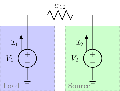
Figure 1: A schematic depiction of a power grid with a single load node and a single source node ($n=m=1$), where $w_{12}$ is the conductance of the line between the nodes.

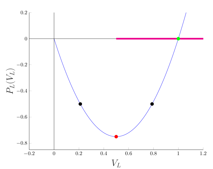
Figure 2: A plot of $P_{L}(V_{L})$ against $V_{L}$ for the power grid in Figure 1 with $w_{12}=3~{}\Omega^{-1}$ and $V_{S}=V_{2}=1~{}\operatorname{V}$. The red point indicates the voltage such that the power that the grid transports is maximized. The thick purple half-line corresponds to $\mathcal{D}$, the set of all long-term voltage stable operating points.

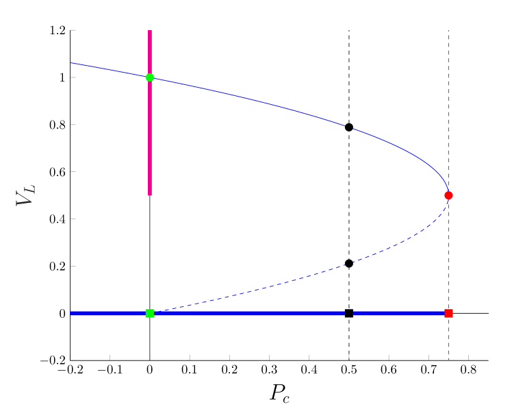
Figure 3: A plot of $V_{L}$ against $P_{c}$ for the power grid in Figure 1 with $w_{12}=3~{}\Omega^{-1}$ and $V_{S}=V_{2}=1~{}\operatorname{V}$. The thick blue half-line corresponds to all feasible power demands at the load node. The red square indicates the maximal power that the load can drain from the power grid. There are multiple operating points if $0<P_{c}<0.75$. The Jacobian $\frac{\partial V_{L}}{\partial P_{c}}$ is not defined in the red point. The corresponding operating point is long-term voltage semi-stable, but not long-term voltage stable. The solid curve depicts a one-to-one correspondence between the feasible power demands and the long-term voltage semi-stable operating points.

Eq. (15) of Example II.14 shows that (9) is not always feasible for each $P_{c}$ for $n=1$. We will show that the same is true for $n>1$ by studying the maximal total amount of power that can be transported to the load nodes.

Definition II.15

For a feasible power demand $P_{c}\in\mathcal{F}$, the total feasible power demand is the sum $\mbb{1}^{\top}P_{c}$ of the power demands at the loads.

Definition II.16

A maximizing feasible power demand is a feasible power demand $P_{\text{max}}\in\mathcal{F}$ that maximizes the total feasible power demand. Thus for all $P_{c}\in\mathcal{F}$ it satisfies

$$\mbb{1}^{\top}P_{c}\leq\mbb{1}^{\top}P_{\text{max}}.$$ (17)

Lemma II.17

There is a unique maximizing feasible power demand $P_{\text{max}}\in\mathcal{F}$. It is given by

$$P_{\text{max}}=\tfrac{1}{4}[V_{L}^{*}]\mathcal{I}_{L}^{*}\gneqq\mbb{0}.$$ (18)

The unique operating point corresponding to $P_{\text{max}}$ is $\tfrac{1}{2}V_{L}^{*}$.

Proof:

Let $P_{c}$ be feasible, and let $V_{L}$ be an associated operating point. Recall from (12) that the total feasible power demand $\mbb{1}^{\top}P_{c}$ satisfies

$$\mbb{1}^{\top}P_{c} =-V_{L}^{\top}Y_{LL}(V_{L}-V_{L}^{*}).$$

By completing the squares we find that

$$\mbb{1}^{\top}P_{c} =-(V_{L}^{*}-\tfrac{1}{2}V_{L})^{\top}Y_{LL}(V_{L}^{*}-\tfrac{1}{2}V_{L})+\tfrac{1}{4}{V_{L}^{*}}^{\top}Y_{LL}V_{L}^{*}.$$

Since $Y_{LL}$ is positive definite, it follows that

$$\mbb{1}^{\top}P_{c}\leq\tfrac{1}{4}{V_{L}^{*}}^{\top}Y_{LL}V_{L}^{*},$$ (19)

with equality if and only if $V_{L}=\tfrac{1}{2}V_{L}^{*}$. This implies that equality in (19) holds if and only if

$$P_{c}=-P_{L}(\tfrac{1}{2}V_{L}^{*})=\tfrac{1}{4}[V_{L}^{*}]Y_{LL}V_{L}^{*}=\tfrac{1}{4}[V_{L}^{*}]\mathcal{I}_{L}^{*},$$

where we have substituted (6). The above implies that there is a unique $P_{\text{max}}$ given by (18), and corresponds to the unique operating point $\tfrac{1}{2}V_{L}^{*}$. Lemma II.3 implies that $P_{\text{max}}\gneqq\mbb{0}$, since $V_{L}^{*}>\mbb{0}$ and $\mathcal{I}_{L}^{*}\gneqq\mbb{0}$. ∎

We remark that if a load node $i$ does not share a line with a source node, then $(\mathcal{I}_{L}^{*})_{i}=(-Y_{LS}V_{S})_{i}=0$, and $P_{\text{max},i}=0$.

The inequality (17) describes a closed half-space in the space of power demands, and is a necessary condition for the feasibility of (9). This condition coincides with the inclusion

$$\mathcal{F}\subseteq\left\{\vphantom{P_{c}\mbb{1}^{\top}P_{c}\leq\mbb{1}^{\top}P_{\text{max}}}\right.P_{c}\left|\vphantom{P_{c}\mbb{1}^{\top}P_{c}\leq\mbb{1}^{\top}P_{\text{max}}}\right.\mbb{1}^{\top}P_{c}\leq\mbb{1}^{\top}P_{\text{max}}\left.\vphantom{P_{c}\mbb{1}^{\top}P_{c}\leq\mbb{1}^{\top}P_{\text{max}}}\right\}.$$ (20)

We observe that (20) generalizes (16) for $n\geq 1$. Since there is a unique maximizing feasible power demand by Lemma II.17, equality in (17) only holds for $P_{\text{max}}$, and the inclusion in (20) strict for $n>1$.

The converse of (17) states that, if $P_{c}$ is such that $\mbb{1}^{\top}P_{c}>\mbb{1}^{\top}P_{\text{max}}$, then no solution to (9) exists. The existence of $P_{\text{max}}$ therefore once more shows that the DC power flow equations with constant-power loads are not always feasible. The following example illustrates (20).

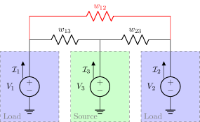
Figure 4: A schematic depiction of a power grid with two load nodes ($n=2$, $m=1$).

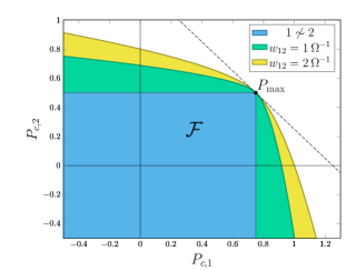
Figure 5: Plots of $\mathcal{F}$, the set of feasible power demands, for the power grid in Figure 4 with different values of $w_{12}$, where $w_{13}=3~{}\Omega^{-1}$, $w_{23}=2~{}\Omega^{-1}$ and $V_{S}=1\operatorname{V}$. The dashed line is the set of the points for which equality in (17) holds.

Example II.18 (two loads, one source case)

Consider the DC power grid with two loads ($n=2$) and one source ($m=1$) depicted in Figure 4. Figure 5 gives the feasible power demands when we let $w_{13}=3\operatorname{\Omega}^{-1}$, $w_{23}=2\operatorname{\Omega}^{-1}$ and $V_{S}=1\operatorname{V}$, and vary the conductance $w_{12}$. It can be shown that $V_{L}^{*}=\mbb{1}\operatorname{V}$.
First, we disregard the red line between node 1 and node 2 (i.e., $1\not\sim 2$), or equivalently take $w_{12}=0\operatorname{\Omega}^{-1}$. The absence of the red line implies that $Y_{LL}$ is (block) diagonal, and Problem II.6 reduces to two copies of Example II.14. From (15) it follows that $P_{c}$ is feasible if and only if $P_{c,1}\leq 0.75$ and $P_{c,2}\leq 0.5$, which corresponds to the blue rectangle in Figure 5. Next, we consider the red line between loads 1 and 2. We observe from the same figure that increasing $w_{12}$ will result in a larger set of feasible power demands, as indicated by the green and yellow areas. The dashed line are the points for which equality in (17) holds. We note that these sets lie below the dashed line, and intersect the line only at the point $P_{\text{max}}$, which illustrates (20). ∎

Figure 6 relates the sufficient conditions of [3] and [6] to the feasible power demands of the DC power grid depicted in Figure 4. Figures 5 and 6 suggest some properties of the set of feasible power demands $\mathcal{F}$, which we will prove in this paper:

• The set $\mathcal{F}$ is convex (M4) (See also [8]).

• Each hyperplane which is tangent to the boundary of $\mathcal{F}$ (such as the dashed line in Figure 5) gives a necessary condition for feasibility (M4) (See also [7]).

• If $y\in\mathcal{F}$ and $\widehat{y}\leq y$, then also $\widehat{y}\in\mathcal{F}$ (M9).

• The convex hull of the points on the boundary of $\mathcal{F}$ lead to a sufficient condition for a power demand to be feasible. In particular, the convex hull of $\mbb{0}$, $P_{\text{max}}$ and the points where the axes intersect the boundary of $\mathcal{F}$ forms a polyhedral subset of $\mathcal{F}$. The interior of this set describes the sufficient condition from [3] (M10). See also Figure 6.

• The ball with the smallest radius such that it touches the boundary of the condition in [3] is contained in $\mathcal{F}$. This subset describes the sufficient condition of [7] (M10); see again Figure 6.

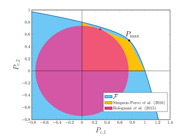
Figure 6: A plot of the set $\mathcal{F}$ for the power grid in Figure 4, where $w_{12}=2~{}\Omega^{-1}$, $w_{13}=3~{}\Omega^{-1}$, $w_{23}=2~{}\Omega^{-1}$ and $V_{S}=1\operatorname{V}$. The yellow area is the set described by the sufficient condition in [3]. The red area is the sufficient condition from [6]. The boundaries of the two conditions intersect in the red point.

We also observe in Figure 5 that $P_{\text{max}}$ does not change when $w_{12}$ is changed, and increasing $w_{12}$ leads to nested sets $\mathcal{F}$ of feasible power demands. We remark that this is not true in general. The analysis of this phenomenon is beyond the scope of this paper.

III A geometric framework for DC power flow feasibility with constant-power loads

In this section we establish a geometric framework for the feasibility of DC power flow with constant-power loads. This section is structured as follows. In Section III-A we show that every operating point is uniquely associated to a Z-matrix: the Jacobian of $P_{c}$ at that operating point. Moreover, we show that an operating point is long-term voltage stable if and only if the Jacobian of $P_{c}$ is a nonsingular M-matrix. Section III-B uses this characterization to obtain a parametrization of the set of long-term voltage stable operating points $\mathcal{D}$. In particular, we parametrize the boundary of $\mathcal{D}$ by a set $\Lambda_{1}$. In Section III-C we study the convex hull of $\mathcal{F}$ and show that $\Lambda_{1}$ also parametrizes the boundary of $\operatorname{conv}(\mathcal{F})$. This establishes a one-to-one correspondence between the boundary of $\mathcal{D}$ and the boundary of $\operatorname{conv}(\mathcal{F})$. Our main results are stated in Section III-D, in which we prove that for each feasible power demand there exists a unique long-term voltage semi-stable operating point. In addition we present an explicit method for computing this operating point and show that the set of feasible power demands is closed and convex. Finally, in Section III-E we prove that the LMI condition in [7] is necessary and sufficient for the feasibility of a vector of power demands, and present a similar necessary and sufficient LMI for the feasibility of a vector of power demands under small perturbation.

III-A Relating operating points to the Jacobian of $P_{c}$

Recall that Z-matrices, M-matrices and irreducible matrices were defined in Definitions I.1-I.3.

Proposition III.1

Let $A$ be an irreducible Z-matrix. There is a unique eigenvalue $r$ of $A$ with smallest (i.e., “most negative”) real part. The eigenvalue $r$, known as the Perron root, is real and simple. A corresponding eigenvector $v$, known as a Perron vector, is unique up to scaling, and can be chosen such that $v>\mbb{0}$.

We include a short proof, as we were unable to find a reference to this result in this exact formulation.

Proof:

Let $B$ be a nonnegative matrix and $s$ a scalar such that $A=sI-B$. Irreducibility is independent of the diagonal elements of a matrix. Hence, since $A$ is irreducible, so is $B$. Let $\rho(B)$ denote the spectral norm of $B$. By the Perron-Frobenius Theorem [12, Thm. 4.8], $\rho(B)$ is a simple eigenvalue of $B$ and there exists a positive eigenvector $v$ so that $Bv=\rho(B)v$. Hence, $r=s-\rho(B)$ is a simple eigenvalue of $A$. The corresponding eigenvector $v$ is unique up to scaling. ∎

Appendix -A lists a number of useful results concerning Z-matrices, M-matrices and irreducible matrices.

The Jacobian of $P_{c}$ at $\widetilde{V}_{L}$ is given by

$$\frac{\partial P_{c}}{\partial V_{L}}(\widetilde{V}_{L})=[Y_{LL}(V_{L}^{*}-\widetilde{V}_{L})]-[\widetilde{V}_{L}]Y_{LL}.$$ (21)

Recall that a vector $\widetilde{V}_{L}$ qualifies as a vector of voltage potentials only if $\widetilde{V}_{L}>\mbb{0}$. The following lemma shows that the matrix (21) has a particular structure if (and only if) $\widetilde{V}_{L}>\mbb{0}$, and that each such matrix is unique for $\widetilde{V}_{L}>\mbb{0}$.

Lemma III.2

The matrix $-\frac{\partial P_{c}}{\partial V_{L}}(\widetilde{V}_{L})$ (i.e., the Jacobian of $-P_{c}$ at $\widetilde{V}_{L}$) is an irreducible Z-matrix if and only if $\widetilde{V}_{L}>\mbb{0}$. The map $\widetilde{V}_{L}\mapsto\frac{\partial P_{c}}{\partial V_{L}}(\widetilde{V}_{L})$ is injective for $\widetilde{V}_{L}>\mbb{0}$.

Proof:

($\Rightarrow$): Let $i\in\boldsymbol{n}$ and note that we have

$$\left(-\tfrac{\partial P_{c}}{\partial V_{L}}(x)\right)_{[i,i^{\mathrm{c}}]}=([x]Y_{LL}-[Y_{LL}(V_{L}^{*}-x)])_{[i,i^{\mathrm{c}}]}\\ =([x]Y_{LL})_{[i,i^{\mathrm{c}}]}=x_{i}(Y_{LL})_{[i,i^{\mathrm{c}}]}.$$ (22)

If $x_{i}=0$, then $\left(-\tfrac{\partial P_{c}}{\partial V_{L}}(x)\right)_{[i,i^{\mathrm{c}}]}=0$ by (22), which violates the irreducibility of the $-\frac{\partial P_{c}}{\partial V_{L}}(x)$. Hence $x_{i}\neq 0$. Since $Y_{LL}$ is a Z-matrix, we have $(Y_{LL})_{[i,i^{\mathrm{c}}]}\leq 0$. Since $Y_{LL}$ is irreducible we know that $(Y_{LL})_{[i,i^{\mathrm{c}}]}\neq 0$, by definition. It follows that there exists at least one negative element in $(Y_{LL})_{[i,i^{\mathrm{c}}]}$. Hence, there exists a $j\neq i$ so that $(Y_{LL})_{ij}<0$. It follows from (22) that

$$\left(-\tfrac{\partial P_{c}}{\partial V_{L}}(x)\right)_{ij}=x_{i}(Y_{LL})_{ij}.$$ (23)

The right-hand side of (23) is nonzero, $(Y_{LL})_{ij}$ is negative, and the left-hand side of (23) is nonpositive since $-\tfrac{\partial P_{c}}{\partial V_{L}}(x)$ is a Z-matrix. This implies that $x_{i}$ is positive. Hence $x>\mbb{0}$.

($\Leftarrow$): The matrix $Y_{LL}$ is an irreducible Z-matrix. Since $x>\mbb{0}$, also $[x]Y_{LL}$ is an irreducible Z-matrix, by 3 and 4 of Proposition .3. Consequently, $[x]Y_{LL}-[Y_{LL}(V_{L}^{*}-x)]$ is an irreducible Z-matrix, by 1 and 2 of Proposition .3.

Let $x,z>\mbb{0}$ satisfy $\frac{\partial P_{c}}{\partial V_{L}}(x)=\frac{\partial P_{c}}{\partial V_{L}}(z)$. By (23) this implies that for all $i$ there exists a $j$ such that $x_{i}(Y_{LL})_{ij}=z_{i}(Y_{LL})_{ij}$. Since $(Y_{LL})_{ij}\neq 0$, it follows that $x_{i}=z_{i}$, and hence $x=z$. ∎

Lemma III.2 states that the Jacobian of $P_{c}$ at an operating point $\widetilde{V}_{L}>\mbb{0}$ is unique to $\widetilde{V}_{L}$. This implies that operating points are uniquely identified by properties of the associated Jacobian. The following result identifies all long-term voltage stable operating points (see Definition II.8) by means of properties of the associated Jacobian.

Proposition III.3

The set $\mathcal{D}$ of long-term voltage stable operating points equals

$$\mathcal{D}=\left\{\vphantom{\widetilde{V}_{L}>\mbb{0}-\frac{\partial P_{c}}{\partial V_{L}}(\widetilde{V}_{L})\text{ is a nonsingular M-matrix}}\right.\widetilde{V}_{L}>\mbb{0}\left|\vphantom{\widetilde{V}_{L}>\mbb{0}-\frac{\partial P_{c}}{\partial V_{L}}(\widetilde{V}_{L})\text{ is a nonsingular M-matrix}}\right.-\frac{\partial P_{c}}{\partial V_{L}}(\widetilde{V}_{L})\text{ is a nonsingular M-matrix}\left.\vphantom{\widetilde{V}_{L}>\mbb{0}-\frac{\partial P_{c}}{\partial V_{L}}(\widetilde{V}_{L})\text{ is a nonsingular M-matrix}}\right\}.$$

Proof:

Let $\widetilde{V}_{L}>\mbb{0}$ be an operating point associated to some vector of power demands $\widetilde{P}_{c}$. Recall from Definition II.8 that $\widetilde{V}_{L}$ is long-term voltage stable if $\frac{\partial P_{c}}{\partial V_{L}}(\widetilde{V}_{L})$ is nonsingular and $\frac{\partial P_{c}}{\partial V_{L}}(\widetilde{V}_{L})^{-1}=\frac{\partial V_{L}}{\partial P_{c}}(\widetilde{P}_{c})$ is a matrix with negative elements. Since $\widetilde{V}_{L}>\mbb{0}$, $-\frac{\partial P_{c}}{\partial V_{L}}(\widetilde{V}_{L})$ is a Z-matrix by Lemma III.2. If follows by [12, Thm. 5.12] that $-\frac{\partial P_{c}}{\partial V_{L}}(\widetilde{V}_{L})^{-1}>0$ if and only if $-\frac{\partial P_{c}}{\partial V_{L}}(\widetilde{V}_{L})$ is a nonsingular M-matrix. ∎

Recall from Definition II.9 that an operating point is long-term voltage semi-stable if it lies in the the closure of $\mathcal{D}$. Proposition III.3 implies the following characterization of such operating points.

Corollary III.4

The closure and boundary of $\mathcal{D}$ satisfies

$$\operatorname{cl}(\mathcal{D}) =\left\{\vphantom{\widetilde{V}_{L}>\mbb{0}-\frac{\partial P_{c}}{\partial V_{L}}(\widetilde{V}_{L})\text{ is an M-matrix}}\right.\widetilde{V}_{L}>\mbb{0}\left|\vphantom{\widetilde{V}_{L}>\mbb{0}-\frac{\partial P_{c}}{\partial V_{L}}(\widetilde{V}_{L})\text{ is an M-matrix}}\right.-\frac{\partial P_{c}}{\partial V_{L}}(\widetilde{V}_{L})\text{ is an M-matrix}\left.\vphantom{\widetilde{V}_{L}>\mbb{0}-\frac{\partial P_{c}}{\partial V_{L}}(\widetilde{V}_{L})\text{ is an M-matrix}}\right\};$$

$$\partial\mathcal{D} =\left\{\vphantom{\widetilde{V}_{L}>\mbb{0}-\frac{\partial P_{c}}{\partial V_{L}}(\widetilde{V}_{L})\text{ is a singular M-matrix}}\right.\widetilde{V}_{L}>\mbb{0}\left|\vphantom{\widetilde{V}_{L}>\mbb{0}-\frac{\partial P_{c}}{\partial V_{L}}(\widetilde{V}_{L})\text{ is a singular M-matrix}}\right.-\frac{\partial P_{c}}{\partial V_{L}}(\widetilde{V}_{L})\text{ is a singular M-matrix}\left.\vphantom{\widetilde{V}_{L}>\mbb{0}-\frac{\partial P_{c}}{\partial V_{L}}(\widetilde{V}_{L})\text{ is a singular M-matrix}}\right\}.$$

The proof follows directly from Proposition .2.

Remark III.5

Many equivalent characterizations of long-term voltage stable operating points may be derived from Proposition III.3. Indeed, the paper [16] lists numerous equivalent conditions for when a Z-matrix is a nonsingular M-matrix. In particular, it follows from property $\mathrm{J}_{29}$ of [16] together with Proposition .3.5 that if $\widetilde{V}_{L}>\mbb{0}$, and hence $-\frac{\partial P_{c}}{\partial V_{L}}(\widetilde{V}_{L})$ is a Z-matrix by Lemma III.2, then $-\frac{\partial P_{c}}{\partial V_{L}}(\widetilde{V}_{L})$ is a nonsingular M-matrix if and only if $[\widetilde{V}_{L}]^{-1}\frac{\partial P_{c}}{\partial V_{L}}(\widetilde{V}_{L})$ is Hurwitz stable. This shows that $\widetilde{V}_{L}>\mbb{0}$ is long-term voltage stable if and only if $[\widetilde{V}_{L}]^{-1}\frac{\partial P_{c}}{\partial V_{L}}(\widetilde{V}_{L})$ is Hurwitz stable. The latter property coincides with the definition of voltage-regularity found in [4]. Alternatively, without invoking Proposition .3.5 it follows that $\widetilde{V}_{L}>\mbb{0}$ is long-term voltage stable if and only if $\frac{\partial P_{c}}{\partial V_{L}}(\widetilde{V}_{L})$ is Hurwitz stable. Similarly it can be shown that $\widetilde{V}_{L}>\mbb{0}$ is long-term voltage semi-stable if and only if $\frac{\partial P_{c}}{\partial V_{L}}(\widetilde{V}_{L})$ is Hurwitz semi-stable.

III-B A parametrization of $\mathcal{D}$

Proposition III.3 and Corollary III.4 allow us to deduce a parametrization for the set $\mathcal{D}$ of all long-term voltage stable operating points. Such a parametrization gives a constructive method to determine where such operating points lie in the voltage domain, as opposed to testing at which operating points of interest the Jacobian of $P_{c}$ is Hurwitz stable (see Remark III.5).

We introduce the following definitions. For a vector $\lambda\in\mathbb{R}^{n}$ we introduce the $n\times n$ matrix

$$h(\lambda):=\tfrac{1}{2}([\lambda]Y_{LL}+Y_{LL}[\lambda]).$$

Note that $h(\mbb{1})=Y_{LL}$, and that

$$x^{\top}h(\lambda)x=x^{\top}[\lambda]Y_{LL}x=\lambda^{\top}[x]Y_{LL}x.$$ (24)

In addition we define the set

$$\Lambda:=\left\{\vphantom{\lambda h(\lambda)\text{ is positive definite}}\right.\lambda\left|\vphantom{\lambda h(\lambda)\text{ is positive definite}}\right.h(\lambda)\text{ is positive definite}\left.\vphantom{\lambda h(\lambda)\text{ is positive definite}}\right\}.$$ (25)

The set $\Lambda$ is studied in Appendix -B. In particular, Lemma .5 shows that $\Lambda$ is convex, and Lemma .6 shows that $\Lambda$ lies in the positive orthant.

The following theorem extends Lemma III.2, and allows us to parametrize the sets $\mathcal{D}$, $\operatorname{cl}(\mathcal{D})$, and $\partial\mathcal{D}$.

Lemma III.6

Let $r\in\mathbb{R}$ and $\lambda\in\mathbb{R}^{n}$ such that $r\geq 0$ and $\lambda>\mbb{0}$. The Jacobian $-\frac{\partial P_{c}}{\partial V_{L}}(\widetilde{V}_{L})^{\top}$ is an irreducible M-matrix with Perron root $r$ and Perron vector $\lambda$ if and only if $h(\lambda)$ is positive definite (i.e., $\lambda\in\Lambda$) and $\widetilde{V}_{L}$ satisfies

$$\widetilde{V}_{L}=\tfrac{1}{2}h(\lambda)^{-1}[\lambda](\mathcal{I}_{L}^{*}+r\mbb{1}),$$ (26)

in which case we have $\widetilde{V}_{L}>\mbb{0}$.

Proof:

($\Rightarrow$): The matrix $Y_{LL}$ is an irreducible Z-matrix and $\lambda>\mbb{0}$, and so $h(\lambda)$ is an irreducible Z-matrix by Propositions .3 and .4. We let $s$ and $v>\mbb{0}$ denote respectively the Perron root and a Perron vector of $h(\lambda)$. The matrix $-\frac{\partial P_{c}}{\partial V_{L}}(\widetilde{V}_{L})^{\top}$ is an M-matrix, and hence a Z-matrix. By Lemma III.2 we have $\widetilde{V}_{L}>\mbb{0}$. Using the fact that $(r,\lambda)$ is an eigenpair to $-\frac{\partial P_{c}}{\partial V_{L}}(\widetilde{V}_{L})^{\top}$, we observe that

$$r\lambda =-\frac{\partial P_{c}}{\partial V_{L}}(\widetilde{V}_{L})^{\top}\lambda=-([Y_{LL}(V_{L}^{*}-\widetilde{V}_{L})]-Y_{LL}[\widetilde{V}_{L}])\lambda$$

$$=-[\lambda]Y_{LL}V_{L}^{*}+[\lambda]Y_{LL}\widetilde{V}_{L}+Y_{LL}[\lambda]\widetilde{V}_{L}$$

$$=-[\lambda]\mathcal{I}_{L}^{*}+2h(\lambda)\widetilde{V}_{L}.$$

By rearranging the terms, it follows that

$$[\lambda]\mathcal{I}_{L}^{*}+r\lambda=2h(\lambda)\widetilde{V}_{L}.$$ (27)

Multiplying (27) by $v^{\top}$ results in

$$v^{\top}([\lambda]\mathcal{I}_{L}^{*}+r\lambda)=2v^{\top}h(\lambda)\widetilde{V}_{L}=2sv^{\top}\widetilde{V}_{L}.$$ (28)

Since $\widetilde{V}_{L}>\mbb{0}$, $v>\mbb{0}$, $\lambda>\mbb{0}$, $r\geq 0$ and $\mathcal{I}_{L}^{*}\gneqq\mbb{0}$, it followsthat the left hand side of (28) is positive. Since $v^{\top}\widetilde{V}_{L}$ is also positive, it follows from (28) that the Perron root $s$ is positive. Hence, $h(\lambda)$ is a nonsingular M-matrix by Proposition .2, and (26) follows from (27). Since $h(\lambda)$ is a symmetric nonsingular M-matrix, it is positive definite and $\lambda\in\Lambda$.

($\Leftarrow$): If $\lambda\in\Lambda$, then $\lambda>\mbb{0}$ by Lemma .6. The rest of the proof follows by reversing the steps of the “$\Rightarrow$”-part. ∎

Lemma III.6 allows for an explicit parametrization of the set $\mathcal{D}$ by $\Lambda$, and without relying on properties of the Jacobian of $P_{c}$. Note that (26) is invariant under scaling of $\lambda$, and hence the vectors $\lambda$ may be normalized. For this purpose we define

$$\Lambda_{1}:=\Lambda\cap\left\{\vphantom{\lambda>\mbb{0}\|\lambda\|_{1}=\mbb{1}^{\top}\lambda=1}\right.\lambda>\mbb{0}\left|\vphantom{\lambda>\mbb{0}\|\lambda\|_{1}=\mbb{1}^{\top}\lambda=1}\right.\|\lambda\|_{1}=\mbb{1}^{\top}\lambda=1\left.\vphantom{\lambda>\mbb{0}\|\lambda\|_{1}=\mbb{1}^{\top}\lambda=1}\right\},$$ (29)

which is a convex set, as it is the intersection of convex sets. Appendix -B lists several properties of the closure of $\Lambda_{1}$.

Theorem III.7 (M1)

The set $\mathcal{D}$ of all long-term voltage stable operating point, its closure $\operatorname{cl}(\mathcal{D})$ and its boundary $\partial\mathcal{D}$ are parametrized by

$$\mathcal{D} =\left\{\vphantom{\tfrac{1}{2}h(\lambda)^{-1}[\lambda](\mathcal{I}_{L}^{*}+r\mbb{1})\lambda\in\Lambda_{1},r>0}\right.\tfrac{1}{2}h(\lambda)^{-1}[\lambda](\mathcal{I}_{L}^{*}+r\mbb{1})\left|\vphantom{\tfrac{1}{2}h(\lambda)^{-1}[\lambda](\mathcal{I}_{L}^{*}+r\mbb{1})\lambda\in\Lambda_{1},r>0}\right.\lambda\in\Lambda_{1},r>0\left.\vphantom{\tfrac{1}{2}h(\lambda)^{-1}[\lambda](\mathcal{I}_{L}^{*}+r\mbb{1})\lambda\in\Lambda_{1},r>0}\right\}$$

$$\operatorname{cl}(\mathcal{D}) =\left\{\vphantom{\tfrac{1}{2}h(\lambda)^{-1}[\lambda](\mathcal{I}_{L}^{*}+r\mbb{1})\lambda\in\Lambda_{1},r\geq 0}\right.\tfrac{1}{2}h(\lambda)^{-1}[\lambda](\mathcal{I}_{L}^{*}+r\mbb{1})\left|\vphantom{\tfrac{1}{2}h(\lambda)^{-1}[\lambda](\mathcal{I}_{L}^{*}+r\mbb{1})\lambda\in\Lambda_{1},r\geq 0}\right.\lambda\in\Lambda_{1},r\geq 0\left.\vphantom{\tfrac{1}{2}h(\lambda)^{-1}[\lambda](\mathcal{I}_{L}^{*}+r\mbb{1})\lambda\in\Lambda_{1},r\geq 0}\right\}$$

$$\partial\mathcal{D} =\left\{\vphantom{\tfrac{1}{2}h(\lambda)^{-1}[\lambda]\mathcal{I}_{L}^{*}\lambda\in\Lambda_{1}}\right.\tfrac{1}{2}h(\lambda)^{-1}[\lambda]\mathcal{I}_{L}^{*}\left|\vphantom{\tfrac{1}{2}h(\lambda)^{-1}[\lambda]\mathcal{I}_{L}^{*}\lambda\in\Lambda_{1}}\right.\lambda\in\Lambda_{1}\left.\vphantom{\tfrac{1}{2}h(\lambda)^{-1}[\lambda]\mathcal{I}_{L}^{*}\lambda\in\Lambda_{1}}\right\}.$$

Furthermore, the map

$$(\lambda,r)\mapsto\tfrac{1}{2}h(\lambda)^{-1}[\lambda](\mathcal{I}_{L}^{*}+r\mbb{1})$$ (30)

from $\Lambda_{1}\times\mathbb{R}_{\geq 0}$ to $\operatorname{cl}(\mathcal{D})$ is a bicontinuous map, and the sets $\mathcal{D}$, $\operatorname{cl}(\mathcal{D})$ and $\partial\mathcal{D}$ are simply connected.

Proof:

Proposition .2 states that a Z-matrix is a (nonsingular/singular) M-matrix if and only if its Perron root $r$ is nonnegative (positive/zero). Proposition III.3 and Corollary III.4 together with Lemma III.6 imply that the vector (26) with $\lambda\in\Lambda$ lies in $\mathcal{D}$, $\operatorname{cl}(\mathcal{D})$ or $\partial\mathcal{D}$ if and only if $r$ in (26) satisfies respectively $r>0$, $r\geq 0$ or $r=0$.

The map (30) is a continuous bijection from $\Lambda_{1}\times\mathbb{R}_{\geq 0}$ to $\operatorname{cl}(\mathcal{D})$, which follows from Lemma III.6 and Corollary III.4. The inverse of the map (30) is described taking $x\in\operatorname{cl}(\mathcal{D})$ and computing the Perron vector $\lambda>\mbb{0}$ and the Perron root $r$ of $-\frac{\partial P_{c}}{\partial V_{L}}(x)$. By Proposition .1, the Perron root and Perron vector of $-\frac{\partial P_{c}}{\partial V_{L}}(x)$ are continuous in $x$. Hence the inverse of the map (30) is also continuous.

The set $\Lambda_{1}\times\mathbb{R}_{\geq 0}$ is convex, and is therefore simply connected, which is a topological property. Topological properties are preserved by bicontinuous maps, and thus $\operatorname{cl}(\mathcal{D})$ is also simply connected. The same holds for $\Lambda_{1}\times\mathbb{R}_{>0}$ and $\Lambda_{1}\times\{0\}$, and hence $\mathcal{D}$ and $\partial\mathcal{D}$ are simply connected. ∎

III-C The convex hull of $\mathcal{F}$ and its boundary

In order to study the set $\mathcal{F}$ of feasible power demands, we will be studying its convex hull and its boundary. In particular, we show that there is a one-to-one correspondence between points in the boundary of $\mathcal{D}$ and points in $\partial\operatorname{conv}(\mathcal{F})$, the boundary of the convex hull of $\mathcal{F}$.

To simplify notation, we define for $\lambda\in\Lambda$ the map

$$\varphi(\lambda):=\tfrac{1}{2}h(\lambda)^{-1}[\lambda]\mathcal{I}_{L}^{*}.$$ (31)

Note that $\varphi(\lambda)$ is invariant under scaling of $\lambda$.

The boundary of $\mathcal{D}$ is by definition the set of the operating points which are long-term voltage semi-stable, but not long-term voltage stable. It follows from Theorem III.7 that $\partial\mathcal{D}$ satisfies

$$\partial\mathcal{D}=\left\{\vphantom{\varphi(\lambda)\lambda\in\Lambda_{1}}\right.\varphi(\lambda)\left|\vphantom{\varphi(\lambda)\lambda\in\Lambda_{1}}\right.\lambda\in\Lambda_{1}\left.\vphantom{\varphi(\lambda)\lambda\in\Lambda_{1}}\right\}=\varphi(\Lambda_{1}).$$ (32)

To study the convex hull of $\mathcal{F}$ and its boundary, we make use of the following two identities involving $P_{c}(V_{L})$.

Lemma III.8

For $x,z\in\mathbb{R}^{n}$ we have

$$P_{c}(x+z)=P_{c}(x)+\frac{\partial P_{c}}{\partial V_{L}}(x)z-[z]Y_{LL}z.$$ (33)

We write out the formula using (10) and use (21):

$$P_{c}(x+z)=[x+z]Y_{LL}(V_{L}^{*}-x-z)=[x]Y_{LL}(V_{L}^{*}-x)$$

$$\quad\quad+[z]Y_{LL}(V_{L}^{*}-x)-[x]Y_{LL}z-[z]Y_{LL}z$$

$$\quad=P_{c}(x)+[Y_{LL}(V_{L}^{*}-x)]z-[x]Y_{LL}z-[z]Y_{LL}z$$

$$\quad=P_{c}(x)+\frac{\partial P_{c}}{\partial V_{L}}(x)z-[z]Y_{LL}z.\hskip 88.00015pt\IEEEQEDclosed$$

The matrix $h(\lambda)$ for $\lambda\in\Lambda$ is positive definite by definition, and therefore induces the vector norm

$$\|x\|_{h(\lambda)}:=\sqrt{x^{\top}h(\lambda)x}.$$ (34)

This vector norm is related to $\lambda^{\top}P_{c}(x)$ for $\lambda\in\Lambda$ by the following lemma.

Lemma III.9

Let $\lambda\in\Lambda$. For each $x\in\mathbb{R}^{n}$ we have

$$\lambda^{\top}P_{c}(x)=\|\varphi(\lambda)\|_{h(\lambda)}^{2}-\|\varphi(\lambda)-x\|_{h(\lambda)}^{2}.$$ (35)

Moreover, we have

$$\lambda^{\top}P_{c}(x)\leq\|\varphi(\lambda)\|_{h(\lambda)}^{2}=\lambda^{\top}P_{c}(\varphi(\lambda)),$$ (36)

with equality if and only if $x=\varphi(\lambda)$. Consequently, we have $P_{c}(x)=P_{c}(\varphi(\lambda))$ if and only if $x=\varphi(\lambda)$.

Proof:

Using (10), (6), (31) and (24), we verify that

$$\lambda^{\top}P_{c}(x) =\lambda^{\top}[x]Y_{LL}V_{L}^{*}-\lambda^{\top}[x]Y_{LL}x$$

$$=x^{\top}[\lambda]\mathcal{I}_{L}^{*}-x^{\top}[\lambda]Y_{LL}x$$

$$=2x^{\top}h(\lambda)\varphi(\lambda)-x^{\top}h(\lambda)x$$

$$=\varphi(\lambda)^{\top}h(\lambda)\varphi(\lambda)-\varphi(\lambda)^{\top}h(\lambda)\varphi(\lambda)$$

$$\quad+2x^{\top}h(\lambda)\varphi(\lambda)-x^{\top}h(\lambda)x$$

$$=\|\varphi(\lambda)\|_{h(\lambda)}^{2}-\|\varphi(\lambda)-x\|_{h(\lambda)}^{2}.$$

Eq. (36) follows from (35) since $\|\varphi(\lambda)-x\|_{h(\lambda)}\geq 0$, with equality if and only if $x=\varphi(\lambda)$. Thus, equality in (36) holds if and only if $x=\varphi(\lambda)$. Finally, if $P_{c}(x)=P_{c}(\varphi(\lambda))$, then $\lambda^{\top}P_{c}(x)=\lambda^{\top}P_{c}(\varphi(\lambda))$ therefore $x=\varphi(\lambda)$. ∎

For a vector $\nu$ such that $\|\nu\|_{1}=1$ and a scalar $s$ we define the closed half-space

$$H(\nu,s):=\left\{\vphantom{y\nu^{\top}y\leq s}\right.y\left|\vphantom{y\nu^{\top}y\leq s}\right.\nu^{\top}y\leq s\left.\vphantom{y\nu^{\top}y\leq s}\right\},$$

which has as boundary the hyperplane

$$\partial H(\nu,s)=\left\{\vphantom{y\nu^{\top}y=s}\right.y\left|\vphantom{y\nu^{\top}y=s}\right.\nu^{\top}y=s\left.\vphantom{y\nu^{\top}y=s}\right\}.$$

The vector $\nu$ is normal to the boundary of the half-space and points outwards.

Definition III.10

A half-space $H(\nu,s)$ is said to support a set $S$ if $S\subseteq H(\nu,s)$ and $\operatorname{cl}(S)\cap\partial H(\nu,s)$ is nonempty. I.e., for a given $\nu$, $s$ is the smallest number so that $S\subseteq H(\nu,s)$. A point in $\operatorname{cl}(S)\cap\partial H(\nu,s)$ is a point of support.

If the half-space $H(\nu,s)$ supports $\mathcal{F}$ and $\widetilde{P}_{c}\in\mathcal{F}$ is a point of support, then $\nu^{\top}\widetilde{P}_{c}$ maximizes $\nu^{\top}P_{c}$ for all $P_{c}\in\mathcal{F}$. For example, let $\nu=\frac{1}{n}\mbb{1}$, then the corresponding supporting half-space is given by (20). The vector $P_{\text{max}}$ is the unique point of support, as was shown in Lemma II.17. See also Figure 5, in which the dashed line corresponds to the boundary of this half-space.

In order to obtain a geometric description of the convex hull of $\mathcal{F}$ we aim to apply the following proposition.

Proposition III.11 (Cor. 11.5.1 of [17])

Let the set $S$ be a subset of $\mathbb{R}^{n}$, then

$$\operatorname{cl}(\operatorname{conv}(S))=\bigcap_{\text{support of }S}H(\nu,s)$$

where the intersection is taken over all half-spaces $H(\nu,s)$ which support $S$.

To apply Proposition III.11 to $\mathcal{F}$, we identify all supporting half-spaces of the set $\mathcal{F}$. We will simultaneously identify the supporting half-spaces of the image of $P_{c}$, which is given by

$$\operatorname{im}P_{c}:=\left\{\vphantom{yP_{c}(x)=y,x\in\mathbb{R}^{n}}\right.y\left|\vphantom{yP_{c}(x)=y,x\in\mathbb{R}^{n}}\right.P_{c}(x)=y,x\in\mathbb{R}^{n}\left.\vphantom{yP_{c}(x)=y,x\in\mathbb{R}^{n}}\right\}$$ (37)

and satisfies the inclusion $\mathcal{F}\subseteq\operatorname{im}P_{c}$.

Theorem III.12

Let $\lambda$ be a vector such that $\|\lambda\|_{1}=1$ and $s$ be a scalar. A half-space $H(\lambda,s)$ supports $\mathcal{F}$ if and only if $\lambda\in\Lambda_{1}$ and $s=\|\varphi(\lambda)\|_{h(\lambda)}^{2}$. The point $P_{c}(\varphi(\lambda))\in\mathcal{F}$ is the unique point of support. Moreover, the supporting half-spaces of the set $\mathcal{F}$ and the image of $P_{c}$ coincide.

The proof of Theorem III.12 can be found in Appendix -C. To simplify notation, we define for $\lambda\in\Lambda$ the half-spaces

$$H_{\lambda} :=H(\lambda,\|\varphi(\lambda)\|_{h(\lambda)}^{2}).$$ (38)

Theorem III.12 states that $H_{\lambda}$ for $\lambda\in\Lambda$ are all supporting half-spaces of $\mathcal{F}$. Proposition III.11 therefore allows us to give a direct formula for the closure of the convex hull of $\mathcal{F}$.

Corollary III.13

The closure of the convex hull of $\mathcal{F}$ is the intersection of all half-spaces $H_{\lambda}$ where $\lambda\in\Lambda$, and is equal to the closure of the convex hull of $\operatorname{im}P_{c}$. I.e.,

$$\operatorname{cl}(\operatorname{conv}(\mathcal{F}))=\operatorname{cl}(\operatorname{conv}(\operatorname{im}P_{c}))=\bigcap_{\lambda\in\Lambda_{1}}\nolimits H_{\lambda}.$$ (39)

Now that we have identified the closure of the convex hull of $\mathcal{F}$, we may also identify the boundary of this set.

Theorem III.14

The map $\lambda\mapsto P_{c}(\varphi(\lambda))$ for $\lambda\in\Lambda_{1}$ is one-to-one and parametrizes the boundary of $\operatorname{conv}(\mathcal{F})$. Moreover, the set $\operatorname{conv}(\mathcal{F})$ is closed.

The proof of Theorem III.14 can be found in Appendix -C.

Corollary III.15

The sets $\Lambda_{1}$, $\partial\mathcal{D}$ and $\partial\operatorname{conv}(\mathcal{F})$ are in one-to-one correspondence. In particular, $P_{c}$ is a one-to-one map from $\partial\mathcal{D}$ to $\partial\operatorname{conv}(\mathcal{F})$.

Proof:

It follows from Theorem III.7 that $\varphi(\lambda)$ is a one-to-one map from $\Lambda_{1}$ to $\partial\mathcal{D}$, and Theorem III.14 states that $\lambda\to P_{c}(\varphi(\lambda))$ is a one-to-one map from $\Lambda_{1}$ to $\partial\operatorname{conv}(\mathcal{F})$. Hence, $P_{c}$ is a one-to-one map from $\partial\mathcal{D}$ to $\partial\operatorname{conv}(\mathcal{F})$. ∎

Corollary III.15 states that a vector of power demands $\widetilde{P}_{c}$ that lies on the boundary the convex hull of $\mathcal{F}$ corresponds uniquely to an operating point $\widetilde{V}_{L}$ which is long-term voltage semi-stable but not long-term voltage stable. The pair $(\widetilde{P}_{c},\widetilde{V}_{L})$ corresponds to a unique $\lambda\in\Lambda_{1}$, and the corresponding hyperplane $\partial H_{\lambda}$ intersects $\operatorname{conv}(\mathcal{F})$ only in the unique point of support $\widetilde{P}_{c}$. Hence, $\partial H_{\lambda}$ is the tangent plane at $\widetilde{P}_{c}$ of the boundary of $\operatorname{conv}(\mathcal{F})$. This is observed in Figure 5 for $\widetilde{P}_{c}=P_{\text{max}}$, $\widetilde{V}_{L}=\frac{1}{2}V_{L}^{*}$ and $\lambda=\tfrac{1}{n}\mbb{1}$, and the same holds for all points on the boundary of $\operatorname{conv}(\mathcal{F})$.

III-D One-to-one correspondence between $\mathcal{F}$ and $\operatorname{cl}(\mathcal{D})$

In this section we use Corollary III.15 to prove that $P_{c}$ is a one-to-one mapping from $\operatorname{cl}(\mathcal{D})$ to $\operatorname{conv}(\mathcal{F})$, and that therefore $\mathcal{F}$ is convex. This means each feasible power demand is uniquely associated to a long-term voltage semi-stable operating point. This operating point can be found by solving an initial value problem. The following lemma is intrumental in proving these results.

Lemma III.16

Let $\widehat{V}_{L}\in\mathcal{D}$, define $\widehat{P}_{c}:=P_{c}(\widehat{V}_{L})\in P_{c}(\mathcal{D})$ and let $\widetilde{P}_{c}\in\operatorname{int}(\operatorname{conv}(\mathcal{F}))$. There exists a unique path $\gamma:[0,1]\to\mathcal{D}$ so that the convex combination of $\widehat{P}_{c}$ and $\widetilde{P}_{c}$ is described by

$$P_{c}(\gamma(\theta))=\theta\widetilde{P}_{c}+(1-\theta)\widehat{P}_{c}.$$ (40)

for $0\leq\theta\leq 1$. The path $\gamma$ solves the initial value problem

$$\dot{\gamma}(\theta)=\left(\frac{\partial P_{c}}{\partial V_{L}}(\gamma(\theta))\right)^{-1}(\widetilde{P}_{c}-\widehat{P}_{c})$$ (41)

with initial value $\gamma(0)=\widehat{V}_{L}$. We have $\widetilde{P}_{c}=P_{c}(\gamma(1))$.

The proof of Lemma III.16 can be found in Appendix -D.

Theorem III.17 (M3)

There is a one-to-one correspondence between the long-term voltage semi-stable operating points $\operatorname{cl}(\mathcal{D})$ and the feasible power demands. I.e., for each $\widetilde{P}_{c}\in\mathcal{F}$ there exists a unique $\widetilde{V}_{L}\in\operatorname{cl}(\mathcal{D})$ which satisfies $\widetilde{P}_{c}=P_{c}(\widetilde{V}_{L})$, implying that $\mathcal{F}=P_{c}(\operatorname{cl}(\mathcal{D}))$. More explicitly, $\widetilde{V}_{L}$ is obtained by solving the initial value problem

$$\dot{\gamma}(\theta)=\left(\frac{\partial P_{c}}{\partial V_{L}}(\gamma(\theta))\right)^{-1}\widetilde{P}_{c}$$ (42)

for $\gamma:[0,1]\to\mathbb{R}^{n}$ with initial value $\gamma(0)=V_{L}^{*}$, where the solution $\gamma$ exists, is unique and satisfies $\gamma(1)=\widetilde{V}_{L}$.

Proof:

Note that $\widetilde{P}_{c}\in\mathcal{F}\subseteq\operatorname{conv}(\mathcal{F})$ and that $V_{L}^{*}\in\mathcal{D}$. Suppose $\widetilde{P}_{c}\in\operatorname{int}(\operatorname{conv}(\mathcal{F}))$. By taking $\widehat{V}_{L}=V_{L}^{*}$ and $\widehat{P}_{c}=P_{c}(V_{L}^{*})=\mbb{0}$ in Lemma III.16, there is a unique $\gamma:[0,1]\to\mathcal{D}$ which solves (42) with $\gamma(0)=V_{L}^{*}$ and which satisfies $\widetilde{P}_{c}=P_{c}(\gamma(1))$. Hence we take $\widetilde{V}_{L}:=\gamma(1)\in\mathcal{D}$. To show that there is a unique $\widetilde{V}_{L}\in\mathcal{D}$ such that $\widetilde{P}_{c}=P_{c}(\widetilde{V}_{L})$, suppose that we have $\widetilde{V}_{L}^{\prime}\in\mathcal{D}$ such that $\widetilde{P}_{c}=P_{c}(\widetilde{V}_{L}^{\prime})$. Then by Lemma III.16 there is a unique $\gamma^{\prime}:[0,1]\to\mathcal{D}$ which solves

$$\dot{\gamma}^{\prime}(\theta)=\left(\frac{\partial P_{c}}{\partial V_{L}}(\gamma^{\prime}(\theta))\right)^{-1}(P_{c}(V_{L}^{*})-\widetilde{P}_{c})$$ (43)

with $\gamma^{\prime}(0)=\widetilde{V}_{L}^{\prime}$, and satisfies $P_{c}(\gamma^{\prime}(1))=P_{c}(V_{L}^{*})=\mbb{0}$. Recall from Proposition III.3 that $\gamma^{\prime}(1)>\mbb{0}$ since $\gamma^{\prime}(1)\in\mathcal{D}$. Since $\mbb{0}=P_{c}(\gamma^{\prime}(1))=[\gamma^{\prime}(1)]Y_{LL}(V_{L}^{*}-\gamma^{\prime}(1))$ and $Y_{LL}$ is nonsingular, this implies that $\gamma^{\prime}(1)=V_{L}^{*}$. But now note that $\widehat{\gamma}(\theta):=\gamma^{\prime}(1-\theta)+V_{L}^{*}-\widetilde{V}_{L}^{\prime}$ is a solution to (42), since $P_{c}(V_{L}^{*})=\mbb{0}$ in (43) and since $\widehat{\gamma}(0)=V_{L}^{*}$. Since (42) has a unique solution, it follows that $\widehat{\gamma}=\gamma$, and in particular $\widetilde{V}_{L}=\gamma(1)=\widehat{\gamma}(1)=\widetilde{V}_{L}^{\prime}$, which proves that $\widetilde{V}_{L}$ is unique. Alternatively, if $\widetilde{P}_{c}\in\partial\operatorname{conv}(\mathcal{F})$ then by Corollary III.15 there exists a unique $\widetilde{V}_{L}\in\partial\mathcal{D}$ such that $\widetilde{P}_{c}=P_{c}(\widetilde{V}_{L})\in P_{c}(\operatorname{cl}(\mathcal{D}))$. It follows from Lemma III.9 that there is no other operating point $\widetilde{V}_{L}^{\prime}$ such that $\widetilde{P}_{c}=P_{c}(\widetilde{V}_{L}^{\prime})$. The operating point $\widetilde{V}_{L}$ is also obtained by the initial value problem (42), which follows from taking the limit $\widetilde{P}_{c}\to\partial\mathcal{D}$ for $\widetilde{P}_{c}\in\operatorname{int}(\operatorname{conv}(\mathcal{F}))$. ∎

The next theorem proves that the set $\mathcal{F}$ of feasible power demands is closed and convex, and gives a geometric characterization of $\mathcal{F}$ in terms of the closed half-spaces $H_{\lambda}$.

Theorem III.18 (M4)

The set $\mathcal{F}$ of feasible power demands is closed and convex. Moreover, the set $\mathcal{F}$ is the intersection of all half-spaces $H_{\lambda}$ with $\lambda\in\Lambda_{1}$ (see (38)), and $\mathcal{F}$ coincides with the image of $P_{c}$. I.e.,

$$\mathcal{F}=P_{c}(\operatorname{cl}(\mathcal{D}))=\operatorname{cl}(\operatorname{conv}(\mathcal{F}))=\bigcap_{\lambda\in\Lambda_{1}}H_{\lambda}=\operatorname{im}P_{c}.$$ (44)

Proof:

We will first prove convexity. By definition we have $P_{c}(\operatorname{cl}(\mathcal{D}))\subseteq\mathcal{F}\subseteq\operatorname{conv}(\mathcal{F})$. Hence it suffices to show that $\operatorname{conv}(\mathcal{F})\subseteq P_{c}(\operatorname{cl}(\mathcal{D}))$. Let $\widetilde{P}_{c}\in\operatorname{conv}(\mathcal{F})$. If $\widetilde{P}_{c}\in\partial\operatorname{conv}(\mathcal{F})$, then Corollary III.15 implies that there exists $\widetilde{V}_{L}\in\partial\mathcal{D}$ such that $\widetilde{P}_{c}=P_{c}(\widetilde{V}_{L})\in P_{c}(\operatorname{cl}(\mathcal{D}))$. Alternatively, if $\widetilde{P}_{c}\in\operatorname{int}(\operatorname{conv}(\mathcal{F}))$, then by Lemma III.16 there exists a path $\gamma:[0,1]\to\mathcal{D}$ such that $\gamma(0)=V_{L}^{*}\in\mathcal{D}$ and (40) holds. In particular, (40) implies that $\widetilde{P}_{c}=P_{c}(\gamma(1))\in P_{c}(\mathcal{D})$. Thus $\operatorname{conv}(\mathcal{F})\subseteq P_{c}(\operatorname{cl}(\mathcal{D}))$, and thus $\mathcal{F}$ is convex. Corollary III.13, Theorem III.14 and the convexity of $\mathcal{F}$ further imply that

$$\bigcap_{\lambda\in\Lambda_{1}}H_{\lambda}=\operatorname{cl}(\operatorname{conv}(\mathcal{F}))=\operatorname{conv}(\mathcal{F})=\mathcal{F}.$$ (45)

Finally we show that $\mathcal{F}=\operatorname{im}P_{c}$. Note that $\mathcal{F}\subseteq\operatorname{im}P_{c}$ by definition. Corollary III.13 proves that $\operatorname{cl}(\operatorname{conv}(\operatorname{im}P_{c}))=\operatorname{cl}(\operatorname{conv}(\mathcal{F}))$. We therefore have

$$\operatorname{cl}(\operatorname{conv}(\operatorname{im}P_{c}))=\operatorname{cl}(\operatorname{conv}(\mathcal{F}))=\mathcal{F}\subseteq\operatorname{im}P_{c}.$$

Since $\operatorname{im}P_{c}\subseteq\operatorname{cl}(\operatorname{conv}(\operatorname{im}P_{c}))$, we have $\mathcal{F}=\operatorname{im}P_{c}$. ∎

Remark III.19

Theorem III.18 shows that the image of $P_{c}$ coincides with $\mathcal{F}$. This means that, if nonpositive voltage potentials would be permitted, then any feasible power demand that is satisfied by nonpositive voltage potentials can also be satisfied by positive voltage potentials. Hence, from a theoretical standpoint, the restriction to positive voltage potentials does not make the set of feasible power demands more conservative.

Due to the convexity of $\mathcal{F}$, Corollary III.15 implies that $\partial\mathcal{D}$ and $\partial\mathcal{F}$ in are one-to-one correspondence. Moreover, Lemma III.9 implies that there are no vectors $x\not\in\partial\mathcal{D}$ such that $P_{c}(x)\in\partial\mathcal{F}$. This implies the following corollary.

Corollary III.20 (M2)

For each $\widetilde{P}_{c}$ on the boundary of $\mathcal{F}$ there exist a unique $\widetilde{V}_{L}\in\mathbb{R}^{n}$ that satisfies (9). All such $\widetilde{V}_{L}$ satisfy $\widetilde{V}_{L}>\mbb{0}$ and form the boundary of $\mathcal{D}$. Hence, there is a one-to-one correspondence between $\partial\mathcal{D}$ and $\partial\mathcal{F}$.

Theorem III.17 and Corollary III.20 immediately imply that there is a one-to-one correspondence between the set $\mathcal{D}$ of long-term voltage stable operating points and the power demands which are feasible under small perturbation, by which we mean that such a power demand $\widetilde{P}_{c}$ is feasible and does not lie on the boundary of $\mathcal{F}$ (i.e., $\widetilde{P}_{c}\in\operatorname{int}(\mathcal{F})$). Consequently, if a power demand is feasible under small perturbation, then there exists a unique long-term voltage stable operating point which satisfies the power flow equation.

Corollary III.21

There is a one-to-one correspondence between the long-term voltage stable operating points $\mathcal{D}$ and the feasible power demands under small perturbations $\operatorname{int}(\mathcal{F})$.

III-E A necessary and sufficient LMI condition for feasibility

We conclude Part I of this paper by restating the geometric characterization of $\mathcal{F}$ in Theorem III.18 in terms of an LMI condition. In the context of Problem II.6, [7] presents a necessary LMI condition for the feasibility of power demands, and states that the LMI condition is also necessary when the set of feasible power demands is closed and convex, as is the case here. The next theorem recovers this result and extends the result for power demands which are feasible under small perturbation.

Theorem III.22 (M5)

A vector $\widetilde{P}_{c}$ of power demands is feasible (i.e., $\widetilde{P}_{c}\in\mathcal{F}$) if and only if there does not exists a positive vector $\nu\in\mathbb{R}^{n}$ such that the $(n+1)\times(n+1)$ matrix

$$\begin{pmatrix}[\nu]Y_{LL}+Y_{LL}[\nu]&[\nu]\mathcal{I}_{L}^{*}\\ ([\nu]\mathcal{I}_{L}^{*})^{\top}&2\nu^{\top}\widetilde{P}_{c}\end{pmatrix}=2\begin{pmatrix}h(\nu)&\tfrac{1}{2}[\nu]\mathcal{I}_{L}^{*}\\ \tfrac{1}{2}([\nu]\mathcal{I}_{L}^{*})^{\top}&\nu^{\top}\widetilde{P}_{c}\end{pmatrix}$$ (46)

is positive definite. Similarly, $\widetilde{P}_{c}$ is feasible under small perturbation (i.e., $\widetilde{P}_{c}\in\operatorname{int}(\mathcal{F})$) if and only if there does not exists a positive vector $\nu\in\mathbb{R}^{n}$ such that (46) is positive semi-definite.

Proof:

We will prove the logical transposition.

($\Leftarrow$): Without loss of generality we assume that $\|\nu\|_{1}=1$. If (46) is positive semi-definite, then $h(\nu)$ is positive semi-definite. It follows from Lemmas .8 and .9 that $h(\nu)$ is an irreducible M-matrix. Let $v>\mbb{0}$ be a Perron vector of $h(\nu)$. Suppose that $h(\nu)$ is singular, then $h(\nu)v=\mbb{0}$ by Proposition .2. However, note that for $t\in\mathbb{R}$ we have

$$\begin{pmatrix}tv\\ 1\end{pmatrix}^{\top}\begin{pmatrix}h(\nu)&\tfrac{1}{2}[\nu]\mathcal{I}_{L}^{*}\\ \tfrac{1}{2}([\nu]\mathcal{I}_{L}^{*})^{\top}&\nu^{\top}\widetilde{P}_{c}\end{pmatrix}\begin{pmatrix}tv\\ 1\end{pmatrix}=tv^{\top}[\nu]\mathcal{I}_{L}^{*}+\nu^{\top}\widetilde{P}_{c},$$

which is a nonconstant line in $t$ since $v^{\top}[\nu]\mathcal{I}_{L}^{*}>0$, and is not bounded from below. This contradicts the assumption that (46) is positive semi-definite. Hence $h(\nu)$ must be positive definite and $\nu\in\Lambda_{1}$. Alternatively, if (46) is positive definite, then $h(\nu)$ is positive definite. If $h(\nu)$ is positive definite, then by the Haynsworth inertia additivity formula ([18], Sec. 0.10) (46) is positive definite (semi-definite) if and only if

$$\nu^{\top}\widetilde{P}_{c}-\tfrac{1}{4}([\nu]\mathcal{I}_{L}^{*})^{\top}h(\nu)^{-1}[\nu]\mathcal{I}_{L}^{*}>(\geq)\>0.$$ (47)

Using (31) and (34), we note that (47) is equivalent to

$$\nu^{\top}\widetilde{P}_{c}>(\geq)\>\tfrac{1}{4}([\nu]\mathcal{I}_{L}^{*})^{\top}h(\nu)^{-1}[\nu]\mathcal{I}_{L}^{*}=\|\varphi(\nu)\|_{h(\nu)}^{2}.$$ (48)

Theorem III.18 implies that $\widetilde{P}_{c}$ is not feasible if and only if there exists $\lambda\in\Lambda$ such that $\widetilde{P}_{c}\not\in\ H_{\lambda}$, or equivalently, $\lambda^{\top}\widetilde{P}_{c}>\|\varphi(\lambda)\|_{\lambda}^{2}$. Thus, if (46) is positive definite, then the strict inequality in (48) holds and $\widetilde{P}_{c}$ is not feasible. Moreover, if equality in (48) holds then

$$\nu^{\top}\widetilde{P}_{c}=\|\varphi(\nu)\|_{h(\nu)}^{2}=\nu^{\top}P_{c}(\varphi(\nu)).$$

Lemma III.9 implies that $\widetilde{P}_{c}=P_{c}(\varphi(\nu))$, and thus $\widetilde{P}_{c}\in\partial\mathcal{F}$ by Theorem III.14. Thus, if (46) is positive semi-definite, then $\widetilde{P}_{c}\not\in\mathcal{F}$ or $\widetilde{P}_{c}\in\partial\mathcal{F}$, and therefore $\widetilde{P}_{c}\not\in\operatorname{int}(\mathcal{F})$.

($\Rightarrow$): The converse is obtained by reversing the steps. ∎

Theorem III.22 presents a necessary and sufficient LMI conditions for the feasibility (under small perturbation) of a DC power grid with constant-power loads. A more common formulation of Theorem III.22 as an LMI condition can be obtained by replacing $[\nu]$ by a positive definite diagonal matrix $D$, and replacing $\nu^{\top}\widetilde{P}_{c}$ by $\mbb{1}^{\top}D\widetilde{P}_{c}$ (cf. [7]).

IV Conclusion of Part I

In Part I of this paper we have studied the power flow feasibility of DC power grids with constant-power loads, and have presented a framework for the analysis of this feasibility problem. Specifically, we have presented a geometric characterization of the feasible power demands in terms of half-spaces, along with necessary and sufficient LMI conditions to check if a vector of power demands is feasible (under small perturbation). In addition, we have given a novel proof for the convexity of the set of feasible power demands. More importantly, we proved that there exists a one-to-one correspondence between the feasible power demands and the long-term voltage semi-stable operating points. This shows that for each feasible power demand there exists a unique operating point which is long-term voltage semi-stable and satisfies the power flow equations. This operating point can be found by solving an initial value problem. The existence and uniqueness of this operating point proves that long-term (semi-)stability can be guaranteed for each feasible power demand. Furthermore, we showed that there exists a one-to-one correspondence between the feasible power demands under small perturbations and the long-term voltage stable operating points.

Our analysis is continued in Part II of this paper, in which we study high-voltage operating points and sufficient conditions for power flow feasibility, among other things.

-A Properties of Z-, M- and irreducible matrices

Proposition .1

The Perron root and Perron vector of an irreducible Z-matrix $A$ are continuous in the elements of $A$.

Proof:

All eigenvalues and any eigenvector corresponding to a simple eigenvalue are continuous in the elements of the corresponding matrix (see [19, 3.1.2] and [19, 3.1.3]). ∎

Proposition .2 ([12, Thm. 5.8])

An irreducible M-matrix is singular if and only if its Perron root is zero, in which case its kernel is spanned by any Perron vector.

Proposition .3

Consider the diagonal matrix $[d]$, $d\in\mathbb{R}^{n}$. The following statements hold:

1. If $A$ is irreducible, then $A+[d]$ is irreducible;

2. If $A$ is a Z-matrix, then $A+[d]$ is a Z-matrix;

3. If $A$ is irreducible and $d>\mbb{0}$, then $A[d]$ are $[d]A$ are irreducible;

4. If $A$ is a Z-matrix and $d>\mbb{0}$, then $A[d]$ are $[d]A$ are Z-matrices;

5. If $A$ is an M-matrix and $d>\mbb{0}$, then $A[d]$ are $[d]A$ are M-matrices;

6. If $A$ is an irreducible M-matrix and $d\gneqq\mbb{0}$, then $A+[d]$ is a nonsingular irreducible M-matrices;

Proof:

Statements 1, 2, 3 and 4 follow directly from the definitions of a Z-matrix and irreducible matrix. Statement 5 is shown in [16]. Statement 6 follows from [20, Cor. 3.9] if $A$ is singular, and is implied by [16, Thm. 1, $\mathrm{A}_{3}$] if $A$ is nonsingular. ∎

Proposition .4

The sum of two irreducible Z-matrices is an irreducible Z-matrix.

Proof:

If $A_{[\alpha,\alpha^{\mathrm{c}}]}\lneqq 0$ and $B_{[\alpha,\alpha^{\mathrm{c}}]}\lneqq 0$ then $(A+B)_{[\alpha,\alpha^{\mathrm{c}}]}\lneqq 0$ for all nonempty $\alpha\subsetneqq\boldsymbol{n}$. ∎

-B Properties of $\Lambda_{1}$ and its closure

Recall from (25) and (29) that $\Lambda$ ($\Lambda_{1}$) is the set of vectors $\lambda$ such that $h(\lambda)=\tfrac{1}{2}([\lambda]Y_{LL}+Y_{LL}[\lambda])$ is positive definite (and ${\|\lambda\|_{1}=1}$).

Lemma .5

The set $\Lambda$ is an open convex cone.

Proof:

The convex combination of positive definite matrices is again positive definite, and the set of all positive definite matrices is open. The result follows since $h(\lambda)$ is linear in $\lambda$. ∎

Lemma .6

The set $\Lambda$ is contained in the positive orthant. I.e., $\lambda>\mbb{0}$ for $\lambda\in\Lambda$.

Proof:

Let $\lambda$ be such that $h(\lambda)$ is positive definite. Recall that the matrix $Y_{LL}$ is positive definite. A matrix is positive definite only if its diagonal elements are positive. The diagonal elements of $Y_{LL}$ and $h(\lambda)$ are respectively given by $(Y_{LL})_{ii}$ and $\lambda_{i}(Y_{LL})_{ii}$, and therefore $(Y_{LL})_{ii}>0$ and $\lambda_{i}(Y_{LL})_{ii}>0$. This implies that $\lambda_{i}>0$ for all $i$. ∎

Lemma .7

The set $\Lambda_{1}$ is a bounded convex set.

Proof:

Let $\lambda\in\Lambda$. Since $\lambda>\mbb{0}$ by Lemma .6, it follows that $\|\lambda\|_{1}=\lambda^{\top}\mbb{1}$. Hence $\Lambda_{1}=\Lambda\cap\left\{\vphantom{\lambda\|\lambda\|_{1}=1}\right.\lambda\left|\vphantom{\lambda\|\lambda\|_{1}=1}\right.\|\lambda\|_{1}=1\left.\vphantom{\lambda\|\lambda\|_{1}=1}\right\}=\Lambda\cap\left\{\vphantom{\lambda\lambda^{\top}\mbb{1}=1}\right.\lambda\left|\vphantom{\lambda\lambda^{\top}\mbb{1}=1}\right.\lambda^{\top}\mbb{1}=1\left.\vphantom{\lambda\lambda^{\top}\mbb{1}=1}\right\}$. The latter expression is an intersection of convex sets (see Lemma .5). Hence $\Lambda_{1}$ is convex. The set $\left\{\vphantom{\lambda\|\lambda\|_{1}=1}\right.\lambda\left|\vphantom{\lambda\|\lambda\|_{1}=1}\right.\|\lambda\|_{1}=1\left.\vphantom{\lambda\|\lambda\|_{1}=1}\right\}$ is bounded and thus $\Lambda_{1}$ is bounded. ∎

Lemma .8

The closure of $\Lambda_{1}$ satisfies

$$\operatorname{cl}(\Lambda_{1})=\left\{\vphantom{\lambda h(\lambda)\text{ is positive semi-definite},\|\lambda\|_{1}=1}\right.\lambda\left|\vphantom{\lambda h(\lambda)\text{ is positive semi-definite},\|\lambda\|_{1}=1}\right.h(\lambda)\text{ is positive semi-definite},\|\lambda\|_{1}=1\left.\vphantom{\lambda h(\lambda)\text{ is positive semi-definite},\|\lambda\|_{1}=1}\right\}.$$

Proof:

Since $\Lambda_{1}$ is nonempty, this follows directly from linearity of $h$, and the fact that the positive semi-definite matrices form the closure of the positive definite matrices.∎

Lemma .9

The set $\operatorname{cl}(\Lambda_{1})$ is contained in the positive orthant. Moreover, the matrix $h(\lambda)$ for $\lambda\in\operatorname{cl}(\Lambda_{1})$ is an irreducible M-matrix.

Proof:

The vectors in $\Lambda_{1}$ are positive, and so the vectors in $\operatorname{cl}(\Lambda_{1})$ are nonnegative. To show that $\operatorname{cl}(\Lambda_{1})$ lies in the positive orthant, it suffices to show that if a vector ${\lambda\in\partial\Lambda_{1}}$ contains zeros, then $Y_{LL}$ is not irreducible, which is a contradiction.

Suppose $\lambda\in\partial\Lambda_{1}$ such that $\lambda_{[\alpha]}=\mbb{0}$ and $\lambda_{[\alpha^{\mathrm{c}}]}>\mbb{0}$ for some nonempty set $\alpha\subseteq\boldsymbol{n}$. Let $w$ be a vector such that $w_{[\alpha^{\mathrm{c}}]}=\mbb{0}$ and $w_{[\alpha]}$ is arbitrary. We therefore have $[\lambda]w=\mbb{0}$. Since $h(\lambda)$ is positive semi-definite, the following inequality holds for every vector $v$ and scalar $\beta$:

$$0\leq(v-\beta w)^{\top}h(\lambda)(v-\beta w)=(v-\beta w)^{\top}[\lambda]Y_{LL}(v-\beta w)\\ =v^{\top}[\lambda]Y_{LL}(v-\beta w)=v^{\top}[\lambda]Y_{LL}v-\beta v^{\top}[\lambda]Y_{LL}w$$ (49)

If $v$ is such that $v^{\top}[\lambda]Y_{LL}w\neq 0$, then (49) is violated when we take $\beta$ such that $\beta v^{\top}[\lambda]Y_{LL}w$ is sufficiently large. It follows that $v^{\top}[\lambda]Y_{LL}w=0$ for all $v$. This implies that

$$[\lambda]Y_{LL}w=\mbb{0}.$$ (50)

The rows of (50) corresponding to $\alpha^{\mathrm{c}}\subseteq\boldsymbol{n}$ satisfy

$$[\lambda_{[\alpha^{\mathrm{c}}]}]((Y_{LL})_{[\alpha^{\mathrm{c}},\alpha]}w_{[\alpha]}+(Y_{LL})_{[\alpha^{\mathrm{c}},\alpha^{\mathrm{c}}]}w_{[\alpha^{\mathrm{c}}]})=\mbb{0}.$$ (51)

Recall that $\lambda_{[\alpha^{\mathrm{c}}]}>\mbb{0}$ and $w_{[\alpha^{\mathrm{c}}]}=\mbb{0}$, and thus (51) implies

$$(Y_{LL})_{[\alpha^{\mathrm{c}},\alpha]}w_{[\alpha]}=\mbb{0}.$$ (52)

Since $w_{[\alpha]}$ is arbitrary, (52) should hold for all $w_{[\alpha]}$, and hence $(Y_{LL})_{[\alpha^{\mathrm{c}},\alpha]}=0$. However, this contradicts the assumption that $Y_{LL}$ is irreducible. We conclude that $\lambda>\mbb{0}$.

Since $Y_{LL}$ is an irreducible Z-matrix and $\lambda>\mbb{0}$, Propositions .3 and .4 imply that $h(\lambda)$ is an irreducible Z-matrix. Since $h(\lambda)$ is positive semi-definite, its eigenvalues are real and nonnegative, and so $h(\lambda)$ is an M-matrix. ∎

Lemma .10

Let $\lambda\in\partial\Lambda_{1}$. For every $v\gneqq\mbb{0}$ in the kernel of $h(\lambda)$ we have $\lambda^{\top}\frac{\partial P_{c}}{\partial V_{L}}(x)v>0$ for all $x\in\mathbb{R}^{n}$.

Proof:

Since $\lambda\in\partial\Lambda_{1}$, the matrix $h(\lambda)$ is singular. By Lemma .9, it is a singular irreducible M-matrix, and its Perron root is zero. The kernel of $h(\lambda)$ is spanned by any Perron vector, by Proposition .2. This implies that $v$ is a Perron vector and $v>\mbb{0}$. Let $x$ be any vector. By substituting (21), we note that $\lambda^{\top}\frac{\partial P_{c}}{\partial V_{L}}(x)v$ is equivalent to

$$\lambda^{\top}\frac{\partial P_{c}}{\partial V_{L}}(x)v=\lambda^{\top}[Y_{LL}V_{L}^{*}]v-\lambda^{\top}([x]Y_{LL}+[Y_{LL}x])v\\ =\lambda^{\top}[\mathcal{I}_{L}^{*}]v-2x^{\top}h(\lambda)v=\lambda^{\top}[\mathcal{I}_{L}^{*}]v,$$ (53)

where we used the fact that $h(\lambda)v=\mbb{0}$. Since $v>\mbb{0}$, $\lambda>\mbb{0}$ and $\mathcal{I}_{L}^{*}\gneqq\mbb{0}$, it follows from (53) that $\lambda^{\top}[\mathcal{I}_{L}^{*}]v>0$. We conclude that $\lambda^{\top}\frac{\partial P_{c}}{\partial V_{L}}(x)v>0$. ∎

-C Proofs concerning Section III-C

Proof of Theorem III.12

($\Leftarrow$): The half-space $H(\lambda,s)$ with $\lambda\in\Lambda_{1}$ and $s=\|\varphi(\lambda)\|_{h(\lambda)}^{2}$ is given by

$$H(\lambda,s)=\left\{\vphantom{y\lambda^{\top}y\leq\|\varphi(\lambda)\|_{h(\lambda)}^{2}}\right.y\left|\vphantom{y\lambda^{\top}y\leq\|\varphi(\lambda)\|_{h(\lambda)}^{2}}\right.\lambda^{\top}y\leq\|\varphi(\lambda)\|_{h(\lambda)}^{2}\left.\vphantom{y\lambda^{\top}y\leq\|\varphi(\lambda)\|_{h(\lambda)}^{2}}\right\}.$$

Since $\lambda\in\Lambda_{1}$, Lemma III.9 states that (36) holds for all $x\in\mathbb{R}^{n}$. This implies that $P_{c}(x)\in H(\lambda,s)$ for all $x\in\mathbb{R}^{n}$, and thus $\operatorname{im}P_{c}\subseteq H(\lambda,s)$. To show that $P_{c}(\varphi(\lambda))$ is the unique point of support, we show that

$$\operatorname{cl}(\operatorname{im}P_{c})\cap\partial H(\lambda,s)=\{P_{c}(\varphi(\lambda))\}.$$ (54)

Let $y\in\operatorname{cl}(\operatorname{im}P_{c})\cap\partial H(\lambda,s)$, then there exists a sequence $\{x_{k}\}_{k\in\mathbb{N}}\in\mathbb{R}^{n}$ such that

$$\lim_{k\to\infty}P_{c}(x_{k})=y.$$ (55)

Since $y\in\partial H(\lambda,s)$, multiplying (55) by $\lambda^{\top}$ yields

$$\lim_{k\to\infty}\lambda^{\top}P_{c}(x_{k})=\lambda^{\top}y=s=\|\varphi(\lambda)\|_{h(\lambda)}^{2}.$$ (56)

It follows from rearranging (56) and applying (35) that

$$0=\lim_{k\to\infty}\left(\|\varphi(\lambda)\|_{h(\lambda)}^{2}-\lambda^{\top}P_{c}(x_{k})\right)\\ =\lim_{k\to\infty}\|\varphi(\lambda)-x_{k}\|_{h(\lambda)}^{2}.$$

Hence $\lim_{k\to\infty}x_{k}=\varphi(\lambda)$, and so (54) holds. This proves that $H(\lambda,s)$ supports $\operatorname{im}P_{c}$, and that $P_{c}(\varphi(\lambda))$ is a point of support. The same is true for $\mathcal{F}$ since $\mathcal{F}\subseteq\operatorname{im}P_{c}$ and $P_{c}(\varphi(\lambda))\in\mathcal{F}$.

($\Rightarrow$): Let $x>\mbb{0}$ be a vector. Let $\lambda$ be such that $\|\lambda\|_{1}=1$ and $\lambda\not\in\Lambda_{1}$, which means that $h(\lambda)$ is not positive definite. We will show that there exists a vector $v\geq\mbb{0}$ such that $\lambda^{\top}P_{c}(x+tv)$ for scalars $t\geq 0$ is not bounded from above. Since $x+tv>\mbb{0}$ for all $t\geq 0$, this implies that the hyperplane $H(\lambda,s)$ does not contain $\mathcal{F}$ for any scalar $s$. The same holds for $\operatorname{im}P_{c}$ since $\mathcal{F}\subseteq\operatorname{im}P_{c}$. Lemma III.8 yields

$$P_{c}(\widehat{x}+tv)=P_{c}(\widehat{x})+t\frac{\partial P_{c}}{\partial V_{L}}(\widehat{x})v-t^{2}[v]Y_{LL}v.$$ (57)

We multiply (57) by $\lambda^{\top}$ and use (24), which implies

$$\lambda^{\top}P_{c}(\widehat{x}+tv)=\lambda^{\top}P_{c}(\widehat{x})+t\lambda^{\top}\frac{\partial P_{c}}{\partial V_{L}}(\widehat{x})v-t^{2}v^{\top}h(\lambda)v.$$ (58)

If $\lambda_{i}<0$ for some $i$, then $e_{i}^{\top}h(\lambda)e_{i}=(Y_{LL})_{ii}\lambda_{i}<0$. Hence, taking $v=e_{i}\gneqq\mbb{0}$ in (58) describes a parabola in $t$ which is not bounded from above. Thus $\lambda^{\top}P_{c}(x)$ is not bounded from above for $t\geq 0$.

If $\lambda\geq\mbb{0}$ and $\lambda\not\in\operatorname{cl}(\Lambda_{1})$ then the matrix $h(\lambda)$ has a negative eigenvalue by Lemma .8. Let $r$ be the eigenvalue of $h(\lambda)$ with the smallest (i.e., most negative) real part. Since $\lambda\geq\mbb{0}$, it follows that $h(\lambda)$ is a Z-matrix. The matrix $h(\lambda)$ is block diagonal, where each block corresponds to an irreducible component of $h(\lambda)$. Let $h(\lambda)_{[\alpha,\alpha]}$ be the irreducible component that corresponds to the negative eigenvalue $r$. The matrix $h(\lambda)_{[\alpha,\alpha]}$ is an irreducible Z-matrix with Perron root $r$ and Perron vector $w>\mbb{0}$. Let $v$ in (58) be such that $v_{[\alpha]}=w$ and $v_{[\alpha^{\mathrm{c}}]}=\mbb{0}$, then $v^{\top}h(\lambda)v=rw^{\top}w<0$. It follows that (58) describes a parabola in $t$ which is not bounded from above. Thus $\lambda^{\top}P_{c}(x)$ is not bounded from above for $t\geq 0$.

Finally, suppose $\lambda\in\partial\Lambda_{1}$, which implies by Lemma .9 that $\lambda>\mbb{0}$ and that $h(\lambda)$ is an irreducible M-matrix. The matrix $h(\lambda)$ is singular since $\lambda\not\in\Lambda_{1}$. Let $v>\mbb{0}$ in (58) be a Perron vector of $h(\lambda)$. Proposition .2 states that $v$ spans the kernel of $h(\lambda)$, and so $v^{\top}h(\lambda)v=0$. By Lemma .10 we know that $\lambda^{\top}\frac{\partial P_{c}}{\partial V_{L}}(x)v>0$. This implies that (58) describes a half-line for $t\geq 0$ which is not bounded from above. Hence, $\lambda^{\top}P_{c}(x)$ is not bounded from above for $t\geq 0$. ∎

Proof of Theorem III.14

The half-spaces $H_{\lambda}$ for $\lambda\in\Lambda_{1}$ are all supporting half-spaces of $\operatorname{conv}(\mathcal{F})$, which follows from (39) of Corollary III.13. Theorem III.12 proves that $P_{c}(\varphi(\lambda))$ is a point of support to $H_{\lambda}$, and that it is unique in the case of $\mathcal{F}$. Theorem 2.15 of [21] states that all boundary points of a convex set are a point of support associated to some supporting half-space. This implies that $P_{c}(\partial\mathcal{D})\subseteq\partial\operatorname{conv}(\mathcal{F})$. We prove equality by showing that there are no other points of support.

Let $y\in\operatorname{cl}(\operatorname{conv}(\mathcal{F}))$. Then there exists a sequence $\{y_{k}\}_{k\in\mathbb{N}}\in\operatorname{conv}(\mathcal{F})$ such that $\lim_{k\to\infty}y_{k}=y$. This means that for $k\in\mathbb{N}$ there exists $x_{k},z_{k}\in\mathbb{R}^{n}$ and scalars $\theta_{k}$ such that $y_{k}=\theta_{k}P_{c}(x_{k})+(1-\theta_{k})P_{c}(z_{k})$ and $0<\theta_{k}<1$. Suppose there exists $\widetilde{\lambda}\in\Lambda_{1}$ so that $y\in\partial H_{\widetilde{\lambda}}$. Hence, $y$ is a point of support associated to $H_{\widetilde{\lambda}}$. We define $s:=\|\varphi(\lambda)\|_{h(\lambda)}^{2}$ and observe that

$$\lim_{k\to\infty}\widetilde{\lambda}^{\top}(\theta_{k}P_{c}(x_{k})+(1-\theta_{k})P_{c}(z_{k}))\\ =\lim_{k\to\infty}\widetilde{\lambda}^{\top}y_{k}=\widetilde{\lambda}^{\top}y=s.$$

Lemma III.9 implies that for all $k$ we have $\widetilde{\lambda}^{\top}P_{c}(x_{k})\leq s$, with equality if and only if $x_{k}=\varphi(\widetilde{\lambda})$, and the same holds for $z_{k}$. This implies that

$$\widetilde{\lambda}^{\top}(\theta_{k}P_{c}(x_{k})+(1-\theta_{k})P_{c}(z_{k}))\leq s.$$ (59)

In order to converge to equality in (59) as $k\to\infty$, we require that either $x_{k}\to\varphi(\widetilde{\lambda})$ and $z_{k}\to\varphi(\widetilde{\lambda})$, $x_{k}\to\varphi(\widetilde{\lambda})$ and $\theta_{k}\to 1$, or $z_{k}\to\varphi(\widetilde{\lambda})$ and $\theta_{k}\to 0$. In all cases it follows that $y=\lim_{k\to\infty}y_{k}=P_{c}(\varphi(\widetilde{\lambda}))$. Hence $P_{c}(\varphi(\widetilde{\lambda}))$ is the unique point of support.

Lemma III.9 implies that if $P_{c}(\varphi(\lambda_{1}))=P_{c}(\varphi(\lambda_{2}))$, then $\varphi(\lambda_{1})=\varphi(\lambda_{2})$. Hence the map $\lambda\to P_{c}(\varphi(\lambda))$ is a one-to-one correspondence between $\Lambda_{1}$ and $\partial\operatorname{conv}(\mathcal{F})$, and $\lambda\to P_{c}(\varphi(\lambda))$ for $\lambda\in\Lambda_{1}$ parametrizes $\partial\operatorname{conv}(\mathcal{F})$.

Note the inclusion

$$\partial\operatorname{conv}(\mathcal{F})=P_{c}(\partial\mathcal{D})\subseteq\mathcal{F}\subseteq\operatorname{conv}(\mathcal{F}),$$

which implies that $\operatorname{conv}(\mathcal{F})$ is closed. ∎

-D Proofs concerning Section III-D

Proof of Lemma III.16

First we show that if a path $\gamma:[0,T]\to\mathcal{D}$ satisfies (41) with $\gamma(0)=\widehat{V}_{L}\in\mathcal{D}$, then (40) holds. Indeed, note that the matrix $\frac{\partial P_{c}}{\partial V_{L}}(\gamma(\tau))$ is invertible for $0\leq\tau\leq T$ since $\gamma(\tau)\in\mathcal{D}$, and note for $0\leq\theta\leq T$ that by the fundamental theorem of calculus we have

$$P_{c}(\gamma(\theta)) =P_{c}(\gamma(0))+\int_{0}^{\theta}\frac{\partial P_{c}}{\partial V_{L}}(\gamma(\tau))\dot{\gamma}(\tau)\mathrm{d}\tau.$$ (60)

Substitution of (41) in (60) yields

$$P_{c}(\gamma(\theta)) =P_{c}(\gamma(0))+\int_{0}^{\theta}(\widetilde{P}_{c}-\widehat{P}_{c})\mathrm{d}\tau.$$ (61)

Eq. (40) follows from (61) since $P_{c}(\gamma(0))=P_{c}(\widehat{V}_{L})=\widehat{P}_{c}$.

To complete the proof it remains to show that a solution $\gamma(\theta)\in\mathcal{D}$ to (41) for $\theta\in[0,1]$ exists and that this solution is unique. Let the map $\psi:\mathcal{D}\to\mathbb{R}^{n}$ be defined by

$$\psi(z):=\left(\frac{\partial P_{c}}{\partial V_{L}}(z)\right)^{-1}(\widetilde{P}_{c}-\widehat{P}_{c}).$$

The map $\psi(z)$ is continuously differentiable since $\frac{\partial P_{c}}{\partial V_{L}}(z)$ is invertible for $z\in\mathcal{D}$. Corollary 8.17 of [22] states that the initial value problem (41) has a unique solution $\gamma:(-\varepsilon,\varepsilon)\to B$ for some $\varepsilon>0$, where $B$ is an open neighborhood of $\widehat{V}_{L}$ which is contained in $\mathcal{D}$. Since $\psi(z)$ is continuous at all $z\in\mathcal{D}$, the solution $\gamma$ can be extended to a maximal interval of existence. Indeed, by the Theorem 8.33 of [22] we extend $\gamma$ so that either (i) $\gamma(\theta)\to\partial\mathcal{D}$, or (ii) $|\gamma(\theta)_{i}|\to\infty$ for some $i\in\boldsymbol{n}$, as $\theta\to\omega$ where $\omega\in\mathbb{R}_{>0}\cup\{+\infty\}$. We will treat cases (i) and (ii) separately.

Case (i)

Let $x\in\partial D$ such that $\gamma(\theta)\to x$ as $\theta\to\omega$ and let $y:=P_{c}(x)$. By continuity of $P_{c}(V_{L})$ it follows that $P_{c}(\gamma(\theta))\to y$ as $\theta\to\omega$. Since $\gamma(\theta)\in\mathcal{D}$ for $0\leq\theta<\omega$, the first part of this proof showed that (40) holds for $0\leq\theta<\omega$. Suppose $\omega=1$, then taking the limit $\theta\to\omega$ in (40) implies that $\widetilde{P}_{c}=P_{c}(\gamma(\omega))=y$, which lies on the boundary of $\mathcal{F}$. This contradicts the fact that $\widetilde{P}_{c}\in\operatorname{int}(\operatorname{conv}(\mathcal{F}))$. Suppose $1>\omega$, then (40) implies that $P_{c}(\gamma(\omega))=y$ is a convex combination of $\widehat{P}_{c}$ and $\widetilde{P}_{c}$. Since $\widehat{V}_{L}\not\in\partial\mathcal{D}$ it follows from Theorem III.14 that $\widehat{P}_{c}\not\in\partial\operatorname{conv}(\mathcal{F})$. Since $\widehat{P}_{c}\in\mathcal{F}$ we therefore have $\widehat{P}_{c}\in\operatorname{int}(\operatorname{conv}(\mathcal{F}))$. Let $\lambda\in\Lambda_{1}$ such that $P_{c}(\varphi(\lambda))=y$, which exists by Theorem III.14, and define $s:=\|\varphi(\lambda)\|_{h(\lambda)}^{2}=\lambda^{\top}P_{c}(\varphi(\lambda))=\lambda^{\top}y$. Note that $\lambda^{\top}\widehat{P}_{c}<s$ and $\lambda^{\top}\widetilde{P}_{c}<s$ since $\widehat{P}_{c},\widetilde{P}_{c}\in\operatorname{int}(\operatorname{conv}(\mathcal{F}))$. But since $y$ is a convex combination of $\widehat{P}_{c}$ and $\widetilde{P}_{c}$, this would imply that $\lambda^{\top}y<s$, which is a contradiction. We conclude that $1<\omega$, and in particular $\gamma(\theta)\in\mathcal{D}$ for $0\leq\theta\leq 1$.

Case (ii)

We will show that $\omega=+\infty$ and that $P_{c}(\gamma(\theta))$ describes a half-line for $0\leq\theta<\infty$. Let $\lambda\in\Lambda_{1}$. Note that $|\gamma(\theta)_{i}|\to\infty$ implies that also $|\varphi(\lambda)_{i}-\gamma(\theta)_{i}|\to\infty$. Therefore also $\|\varphi(\lambda)-\gamma(\theta)\|_{h(\lambda)}\to\infty$. It follows from Lemma III.9 that $\lambda^{\top}P_{c}(\gamma(\theta))\to-\infty$. This holds for all $\lambda\in\Lambda_{1}$ and so $P_{c}(\gamma(\theta))$ does not intersect the boundary of $\mathcal{F}$ for $0\leq\theta<\omega$. The first part of this proof showed that (40) holds for $0\leq\theta<\omega$, which describes a half-line in $\theta$. Since $\lambda>\mbb{0}$ by Lemma .6, it follows from $\lambda^{\top}P_{c}(\gamma(\theta))\to-\infty$ that $P_{c}(\gamma(\theta))_{j}\to-\infty$ for some $j\in\boldsymbol{n}$. As a result, (40) implies that $\omega=+\infty$. In particular it follows that $\widetilde{P}_{c}$ lies on the half-line and that $\gamma(\theta)\in\mathcal{D}$ for $0\leq\theta\leq 1$.

To show uniqueness, we note again that $\psi(z)$ is continuously differentiable. Corollary 8.17 of [22] states that (41) has a unique solution in an open neighborhood around any given initial value in $\mathcal{D}$. Taking any point $\gamma(\theta)$ with $0\leq\theta\leq 1$ as an initial value shows that the solution $\gamma$ is unique at each point, and hence is unique in $\mathcal{D}$.

Since (40) holds for $0\leq\theta\leq 1$, (40) implies that $\widetilde{P}_{c}=P_{c}(\gamma(1))\in P_{c}(\mathcal{D})$. ∎

References

- [1] T. Van Cutsem and C. Vournas, Voltage stability of electric power systems. Springer Science & Business Media, 2008.
- [2] U. Eminoglu and M. H. Hocaoglu, “A new power flow method for radial distribution systems including voltage dependent load models,” Electric Power Systems Research, vol. 76, no. 1, pp. 106 – 114, 2005.
- [3] J. W. Simpson-Porco, F. Dörfler, and F. Bullo, “Voltage collapse in complex power grids,” Nature Communications, vol. 7, no. 10790, 2016.
- [4] A. S. Matveev, J. E. Machado, R. Ortega, J. Schiffer, and A. Pyrkin, “A tool for analysis of existence of equilibria and voltage stability in power systems with constant power loads,” IEEE Transactions on Automatic Control, vol. 65, no. 11, pp. 4726–4740, 2020.
- [5] F. Dörfler, M. Chertkov, and F. Bullo, “Synchronization in complex oscillator networks and smart grids,” Proceedings of the National Academy of Sciences, vol. 110, no. 6, pp. 2005–2010, 2013.
- [6] S. Bolognani and S. Zampieri, “On the existence and linear approximation of the power flow solution in power distribution networks,” IEEE Transactions on Power Systems, vol. 31, no. 1, pp. 163–172, 2015.
- [7] N. Barabanov, R. Ortega, R. Griñó, and B. Polyak, “On existence and stability of equilibria of linear time-invariant systems with constant power loads,” IEEE Transactions on Circuits and Systems I: Regular Papers, vol. 63, no. 1, pp. 114–121, Jan 2016.
- [8] A. Dymarsky, “On the convexity of image of a multidimensional quadratic map,” arXiv preprint arXiv:1410.2254, 2014.
- [9] F. Dörfler and F. Bullo, “Novel insights into lossless ac and dc power flow,” in 2013 IEEE Power Energy Society General Meeting, 2013, pp. 1–5.
- [10] J. W. Simpson-Porco, F. Dörfler, and F. Bullo, “A solvability condition for reactive power flow,” in 2015 54th IEEE Conference on Decision and Control (CDC), 2015, pp. 2013–2017.
- [11] A. Dymarsky and K. Turitsyn, “Convexity of solvability set of power distribution networks,” IEEE Control Systems Letters, vol. 3, no. 1, pp. 222–227, Jan 2019.
- [12] M. Fiedler, Special matrices and their applications in numerical mathematics. Kluwer Academic Publishers, 1986.
- [13] A. van der Schaft, “Characterization and partial synthesis of the behavior of resistive circuits at their terminals,” Systems & Control Letters, vol. 59, no. 7, pp. 423 – 428, 2010.
- [14] A. van der Schaft, “The flow equations of resistive electrical networks,” in Interpolation and Realization Theory with Applications to Control Theory: In Honor of Joe Ball. Springer International Publishing, 2019, pp. 329–341.
- [15] W. Rudin et al., Principles of mathematical analysis. McGraw-Hill New York, 1964, vol. 3.
- [16] R. Plemmons, “M-matrix characterizations I - nonsingular M-matrices,” Linear Algebra and its Applications, vol. 18, no. 2, pp. 175 – 188, 1977.
- [17] R. T. Rockafellar, Convex analysis. Princeton University Press, 1970, vol. 28.
- [18] F. Zhang, The Schur complement and its applications. Springer Science & Business Media, 2006, vol. 4.
- [19] J. M. Ortega, Numerical analysis: a second course. SIAM, 1990.
- [20] W. Li, “Characterizations of singular irreducible m-matrices,” Linear and Multilinear Algebra, vol. 38, no. 3, pp. 241–247, 1995.
- [21] F. A. Valentine, Convex sets. McGraw-Hill New York, 1964.
- [22] W. G. Kelley and A. C. Peterson, The theory of differential equations: classical and qualitative. Springer Science & Business Media, 2010.