Homography Estimation with Convolutional Neural Networks Under Conditions of Variance

Abstract

Planar homography estimation is foundational to many computer vision problems, such as Simultaneous Localization and Mapping (SLAM) and Augmented Reality (AR). However, conditions of high variance confound even the state-of-the-art algorithms. In this report, we analyze the performance of two recently published methods using Convolutional Neural Networks (CNNs) that are meant to replace the more traditional feature-matching based approaches to the estimation of homography. Our evaluation of the CNN based methods focuses particularly on measuring the performance under conditions of significant noise, illumination shift, and occlusion. We also measure the benefits of training CNNs to varying degrees of noise. Additionally, we compare the effect of using color images instead of grayscale images for inputs to CNNs. Finally, we compare the results against baseline feature-matching based homography estimation methods using SIFT, SURF, and ORB. We find that CNNs can be trained to be more robust against noise, but at a small cost to accuracy in the noiseless case. Additionally, CNNs perform significantly better in conditions of extreme variance than their feature-matching based counterparts. With regard to color inputs, we conclude that with no change in the CNN architecture to take advantage of the additional information in the color planes, the difference in performance using color inputs or grayscale inputs is negligible. About the CNNs trained with noise-corrupted inputs, we show that training a CNN to a specific magnitude of noise leads to a “Goldilocks Zone” with regard to the noise levels where that CNN performs best.

1 Introduction

A homography is a planar projective transformation represented by a $3\times 3$ non-singular matrix in the homogeneous coordinate system. The matrix H maps homogeneous coordinates x to $\textbf{x}^{\prime}$. This transformation is foundational to many computer vision problems, including Simultaneous Localization and Mapping (SLAM), 3D reconstruction, Augmented Reality (AR), etc. [4] [19] Failing to accurately estimate a homography, especially in non-ideal conditions for automated applications, can cause significant error that propagates through the system. For example, in AR applications that require tracking the pose of a camera, even “minor” camera motions create estimation error that cause state-of-the-art systems to fail [12].

The baseline homography estimation algorithms depend on detecting features in a pair of images, determining candidate feature correspondences by comparing the descriptor vectors associated with the features, eliminating the outliers in the candidate correspondences with RANSAC [5], and, finally, using a nonlinear least-squares method (like the Levenberg-Marquardt algorithm) over the inlier set to estimate the homography. Commonly used algorithms for feature detection and description include Scale Invariant Feature Transform (SIFT) [13], Speeded Up Robust Features (SURF) [1], and Oriented FAST and Rotated BRIEF (ORB) [17]. While these algorithms have been used in various applications for over a decade, they all produce inaccurate results under non-ideal conditions. Noise, illumination variance, and obscuration are common occurrences in many automated computer vision applications that are vulnerable to the erroneous estimations of homography as produced by the feature-matching based methods.

The recent success of Convolutional Neural Networks (CNNs) in computer vision applications has inspired research in using deep learning for homography estimation. In computer vision, CNNs have achieved immense success at object detection and classification, image synthesis, and stereo matching [18] [6] [7]. Against these advances in deep-learning based solutions to computer vision problems, this report presents an exhaustive evaluation of two CNN based tools for estimating homographies [3] [15]. The authors of these two networks have reported significant improvements over what can be achieved with the traditional homography estimation methods using the ORB [17] features.

The CNN-based homograpahy estimation solution presented in [3] uses an altered version of the VGG-14 [11] architecture to calculate the four point parameterization of the homography matrix between an image and a warped image. They used the Common Objects in Context (COCO) Dataset [11] for training and testing. A key part of their method is the process they employed for generating the training data, in which they warped an image with a randomly generated homography, and then passed that homography as the ground truth. The reported results were approximately 20% more accurate than those based on the feature-matching method using ORB.

The second CNN-based homograpahy estimation solution, presented in [15], uses multiple Siamese CNNs in a sequence with an attempt to achieve accuracies better than those reported in [3]. With the “boosting-like” effect achieved by their architecture, they claimed a 67% error reduction compared to what could be achieved with the feature-based method using ORB.

Our main focus in this paper is the analysis of the performance of the CNN based approaches for homography estimation under conditions of high variance — that is, when the image data is corrupted with varying amounts of noise, with varying degrees of illumination changes, and with varying degrees of occlusion. In addition to comparing the two CNN based approaches with each other, we also report on their comparison with the baseline methods based on SIFT, SURF, and ORB.

With regard to noise, of particular significance in our comparative evaluations is the effect on performance when the CNNs are trained on noise-corrupted data vis-a-vis the case when they are trained on just clean data. When the CNNs are trained with noise-corrupted inputs, we show that training a CNN at a specific level of noise leads to a “Goldilocks Zone” with regard to the noise level where that CNN performs best. That is, the CNN-based homography estimator produces the best average performance when the noise level (as characterized by its statistical properties) that was used during the training matches the noise level in the images on which the CNN is tested.

Our comparative evaluation also includes results on color images. That part of the evaluation has required modifying slightly the CNNs proposed in [3] and [15] since now we must account for the three color planes at the input to the CNNs. For the case of color, we show that, with the same overall CNN architecture, the additional information in the color planes makes negligible contributions to the accuracies of the estimated homographies, implying that, perhaps, with additional channels in the convolutional layers — especially those that are closer to the input — one might be able to enhance the accuracies.

All our tests were conducted on the Open 2019 Dataset [10] [9], which is the first attempt at using this dataset for homography estimation with CNNs. We find that, although SIFT is more accurate under ideal conditions, CNNs perform significantly better under conditions of variance, especially with regard to additive noise. We also show that the performance of a CNN-based homography estimator for noisy images can be improved if the CNN is trained with noisy training data containing roughly the same level of noise as is expected in the test data. This improvement vis-a-vis the noise comes at a small cost to the performance for the noiseless case. The key takeaway from our paper is that no one method should be treated as “universally superior” to all others, but instead environmental conditions and engineering constraints need to be deliberately considered when choosing the best method for any application.

In the rest of this paper, we start in Section 2 with a review of the two CNN-based homography estimators mentioned above. We talk about the datasets and the metrics used in our comparative evaluation in Section 3. In Section 4, we describe the experiments we have carried out for meeting the goals of this paper. Section 5 presents the results of our comparative evaluation. Finally, we conclude in Section 6.

2 Homography Estimation With CNNs

In this section, we provide a brief review of the two CNN-based approaches to homography estimation that we have used in our comparative evaluation.

2.1 Deep Image Homography Estimation (DH)

Figure 1: Deep Homography Estimation Model [3]

The CNN-based approach to homography estimation as proposed in [3] uses the VGG-14 Net [18] to process two patches from an image pair. The two input patches are converted to grayscale, normalized, and then are stacked onto each other. The architecture uses eight convolutional layers, followed by two fully connected layers (Figure 1). The convolutional layers use a $3\times 3$ kernel. ReLu activation and batch normalization follows each layer. Max Pooling occurs prior to the third, fifth, and seventh convolutional layers. Dropout with a factor of 0.5 is applied before each fully connected layer.

The output of the neural network is a parameterized form of the homography matrix — the parameterized form is known as the four-point parameterization and denoted $\textbf{H}_{4pt}$. To avoid confusion in the rest of the paper, we will use $\textbf{H}_{mat}$ to denote the original homography matrix and $\textbf{H}_{4pt}$ its four-point parameterization. Using homogeneous coordinates, if x is a point in one image and $\textbf{x}^{\prime}$ the corresponding point in the other image, the two are related by $\textbf{x}^{\prime}=\textbf{H}_{mat}\textbf{x}$. If the relationship between homogeneous coordinates and the actual pixel coordinates is given by $\begin{bmatrix}x_{1}&x_{2}&x_{3}\end{bmatrix}=\begin{bmatrix}u&v&1\end{bmatrix}$ , we can write the following form for the matrix $\textbf{H}_{4pt}$:

$$\textbf{H}_{4pt}=\begin{bmatrix}u_{1}-u_{1}^{\prime}&v_{1}-v_{1}^{\prime}\\ u_{2}-u_{2}^{\prime}&v_{2}-v_{2}^{\prime}\\ u_{3}-u_{3}^{\prime}&v_{3}-v_{3}^{\prime}\\ u_{4}-u_{4}^{\prime}&v_{4}-v_{4}^{\prime}\end{bmatrix}$$ (1)

where $(u_{i},v_{i}),i=1,2,3,4$ are the pixel coordinates of some four corners in one image and $(u_{i}^{\prime},v_{i}^{\prime}),i=1,2,3,4$ the corresponding four corners in the other image. By adding the elements of $\textbf{H}_{4pt}$ to the coordinates of the corners in the first image of an image pair, we obtain the coordinates of the corresponding points in the second image. We can subsequently use the pixel coordinates of the four corresponding corners to calculate $\textbf{H}_{mat}$ from $\textbf{H}_{4pt}$.

The training of the CNN in [3] is done through a self-supervised method in which a patch is randomly selected from the image, no closer than $\rho$ pixels from any image edge. A random perturbation (of no more than $\rho$ pixels) is applied to the corners of the patch, creating warped corners. The correspondences between the original corners and warped corners are used to calculate a homography, $\textbf{H}_{mat}$. The homography is applied to the image, and a patch (from same coordinates as original patch) is extracted from the warped image as the warped patch. The original and warped patches are stacked and input into the neural network, with the corner perturbation values used as the ground truth, $\textbf{H}_{4pt}^{target}$. This “label on the fly” method is both simple and flexible. The ability to use any image dataset for training and testing makes this a powerful approach for homography estimation.

2.2 Homography Estimation with Hierarchical Convolutional Networks (HH)

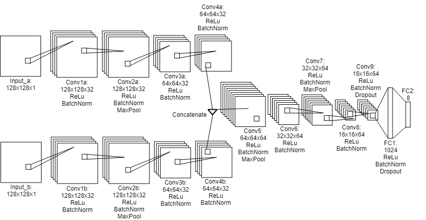
Figure 2: Hierarchical Homography Model [15]

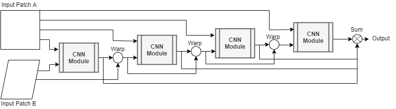
Figure 3: Hierarchical Homography Stack [15]

The CNN-based approach for homography estimation as presented in [15] attempts to improve on the accuracy achievable by the previous approach by using multiple Siamese CNNs stacked end-to-end. Much like the previous CNN based method, this method also takes for input the two image patches and outputs the estimated corner perturbation values $\textbf{H}_{4pt}$, which can be mapped to a homography matrix $\textbf{H}_{mat}$.

This CNN architecture also uses eight convolutional layers followed by two fully connected layers (Fig. 2). However, the first four convolutional layers are two parallel branches with shared weights. The first branch takes the original patch as input, and the second branch takes the warped patch, as opposed to stacking the patches and inputting into the same layer. The branches merge after the fourth layer, concatenating along the feature dimension. Each layer is followed by ReLu activation and batch normalization. Max Pooling is applied after the second, fifth, and seventh convolutional layers. Dropout of factor 0.5 is applied prior to the first fully connected layer.

This architecture is repeated through separate modules stacked end-to-end as shown in Fig. 3. The original patch and the corresponding warped patch are fed into the first module, which estimates $\textbf{H}_{4pt}$. That estimated homography is subtracted from the target to create a new target for the next module.

$$\textbf{H}_{i}^{target}=\textbf{H}_{i-1}^{est}-\textbf{H}_{i}^{target}$$ (2)

The new target is used to create a new warped patch. The input data to the following module is the original patch and new warped patch, with the new target as ground truth. (I represents the input image patch.)

$$(\textbf{I}_{i}^{original},\textbf{I}_{i}^{warped})=(\textbf{I}_{i-1}^{original},\textbf{I}_{i-1}^{original}*\textbf{H}_{i}^{target})$$ (3)

This process is repeated iteratively, with a “boosting” like effect that drives the error down. In other words, the magnitude of the error residuals shrinks between each iteration. By training each module specific to those error residual ranges, the overall accuracy is increased.

3 Dataset Used and the Metrics for the Comparative Evaluation

Our study is based on the Open Images 2019 Test Set (approximately 100k images) [10] [9]. This is the first published use of CNNs for homography estimation on the Open Images Dataset. Additionally, we use the COCO 2017 Unlabeled Dataset (approximately 123k images) [11] for CNN training and validation. By using a different dataset for training/validation and for testing, we ensured that the CNNs generalized appropriately.

The primary metric for testing accuracy was Average Corner Error. This is the Euclidean distance between corner locations after applying the target and output homographies. The value was averaged over the four corners.

$$\begin{split}ACE=\frac{1}{4}\sum_{i=1}^{4}||\textbf{H}_{mat}^{target}\textbf{x}_{i}-\textbf{H}_{mat}^{output}\textbf{x}_{i}||\\ \end{split}$$ (4)

Here, $\textbf{x}_{i}$ refers to one of the four corners of the original patch, $\textbf{H}_{mat}^{target}$ is the ground truth homography in the original matrix parameterization, and $\textbf{H}_{mat}^{output}$ is the estimated homography from the technique being evaluated.

We present median ACE as opposed to mean ACE due to the unbounded error at the positive extreme. The ACEs of the highest error greatly skew the mean. This skewing effect heavily favors CNNs and fails to illustrate which method is most accurate for the majority of the data.

Previous publications on homography estimation with deep learning did not report on how the error is distributed over the dataset for each method [3] [15]. Therefore, in this report we also include a novel metric named Outlier Ratio (OR). This is the ratio of extremely high outlier ACE values compared to the rest of the dataset. For the sake of consistency, we define a value to be an outlier if it exceeds an ACE of 50 pixels, or is undefined because the feature-matching method failed to produce enough correspondences for a solution. We choose 50 since it is such extreme error that if a homography maps points that are greater than 50 pixels away from ground truth in an image patch of size $128\times 128$, that estimated homography has little practical use. This OR metric can be heuristically thought of as the rate at which a certain method will produce a practically unusable homography in given conditions.

4 Setting Up the Experiments for Comparative Evaluation

We implemented and analyzed the performance of the two deep learning solutions under conditions including those of high variance. And we have also compared the performance obtained with the deep-learning based methods with the baseline method that derive a homography using the interest points generated by using the SIFT, SURF, and ORB operators.

We execute the homography estimation tests for all methods on the Open Images 2019 Test Set [10] [9]. Using this dataset, we conduct four experiments by simulating different conditions of variance, including the ideal (i.e. unaltered input images), noise, illumination shifts, and random occlusions.

In addition to the performance evaluations mentioned above, we chose the DH method for evaluating the CNN-based homography estimation when the CNN is trained on noisy data itself. The DH method was chosen for such experiments because the architecture is the same as that of the widely used VGG network, which makes it more likely that the trends found with DH-based experiments are more likely to be experienced with other common CNNs. On the other hand, the HH network uses a Siamese architecture in a sequentially modular layout, which makes HH harder and longer to train and makes it more challenging to select the best hyperparameters for convergence.

We also trained DH on color images (which required making slight modifications to the network).

All training and validation for CNNs was conducted on the COCO Unlabeled 2017 Dataset [11].

As mentioned earlier, the performance was measured with the Average Corner Error (ACE), as well as the Outlier Ratio (OR). Finally, we report the results in tables comparing ACE and OR, as well as figures illustrating the distribution of sorted ACE values for each method per experiment.

4.1 Implementation

As mentioned in the Introduction, in addition to comparing the two deep-learning method for homography estimation, we also compare them with the traditional baseline methods that estimate homographies using the interest points returned by the SIFT, SURF, and ORB operators. For these operators, we used OpenCV 3’s [2] default implementation. After determining correspondences, we solve the homography and refine it with RANSAC.

We implemented and trained the neural networks using the PyTorch library [16]. Labels were created “on the fly” per the method developed in [3] during training and validation. We used the Adam optimizer [8] for both networks, training for approximately 30 epochs at a learning rate of 0.005. (One epoch here is defined as a single pass over the entire training dataset.) The learning rate was halved every five epochs. PyTorch’s MSELoss function was used as the loss function.

4.2 Evaluation Experiments

We conducted four experiments over the entire dataset. Each experiment simulates a different form of variance experienced in natural conditions. The four experiments are Ideal Conditions (where the dataset is unaltered), Gaussian Noise, Illumination Shift, and Occlusion. For the latter three experiments, the process is repeated three times with different variance values to better illustrate the sensitivity of each method as the variance increases. Table 1 breaks down each experiment with the variance values.

To simulate noise, we added normal Gaussian noise scaled by a factor $\eta$ (such as 0.4) relative to pixel range, and clipped the results to normalized pixel range.

$$\begin{split}X_{noisy}=min(max(X+\eta\mathcal{N}(0,1),-1),1)\end{split}$$ (5)

To simulate illumination, we multiplied the pixel values in the warped patch by a factor $\lambda$ (such as 1.4) and clip the results to normalized pixel range.

$$\begin{split}X_{illum}=min(max(\lambda X,-1),1)\end{split}$$ (6)

To simulate occlusions, We replaced an $n\times n$ box of random location with a random color in the warped image. The size of $n\times n$ is determined by a factor $\alpha$ (such as 0.6) relative to the total patch space.

Experiment	Magnitude of Variance
Ideal Conditions	No Variance
Gaussian Noise	$\eta=0.1$	$\eta=0.3$	$\eta=0.5$
Illumination Shift	$\lambda=1.2$	$\lambda=1.4$	$\lambda=1.6$
Occlusion	$\alpha=0.2$	$\alpha=0.4$	$\alpha=0.6$

Table 1: Experiments for investigating the performance of CNN-based homography estimation under four types of variance. In each experiment (except for Ideal), three different magnitudes of variance are used to better illustrate the sensitivity of each method.

After comparing CNNs to the baseline feature matching methods, we analyzed the affect of training on noisy data will have on performance. We used the trained Deep Image Homography Net, train it for an additional 30 epochs in $\eta=0.1$ noisy data, and then measure performance. We then train it for another 30 epochs on $\eta=0.3$, tested again, and then repeat with $\eta=0.5$.

Finally, to measure the effect of using color images instead of grayscale images for input, we modified the Deep Image Homography Net to accept six channels for input instead of two. We then train the network from scratch on color images, and measure performance against the grayscale counterpart.

5 Results of Comparative Evaluation

We illustrate our results with tables depicting the median ACE and OR values for each method under a specific variance. We also present figures that compare the sorted ACE values as line charts for each method in each experiment. This best illustrates the distribution of error over the dataset, and therefore conveys a qualitative sense of consistency. The lines depict sorted ACE values, from least to greatest, for each input patch pair. For brevity, DH refers to the CNN based method described in Section 2.1 and HH refers to the CNN based method described in Section 2.2. In the tables below, the best ACE is in bold. The methods above the dotted line are CNNs, and the methods below are feature matching.

5.1 Ideal Conditions

Under ideal conditions, meaning that when the dataset is unaltered, as shown in Table 2, SIFT gives superior performance for 90% of the dataset. It has sub-pixel ACE for approximately half the dataset. HH is the most consistent, remaining below an ACE of 50 for over 99% of the dataset.

Method	Median ACE	OR
DH	3.97	0
HH	2.25	0.01
SIFT	0.89	0.08
SURF	3.15	0.09
ORB	7.82	0.12

Table 2: Median ACE and OR in Ideal Conditions. SIFT has the lowest median ACE, followed by HH. ORB was the worst-performing method, with a high median ACE and OR.

Fig. 4 shows the plots of the ACE values achieved with all five approaches to homography estimation, the three traditional methods based SIFT, SURF, and ORB, and the two CNN based methods. As is evident from the plot, the feature-matching approach based on SIFT produces the most accurate homographies for 90% of the dataset. However, when it fails for the rest of the dataset, it fails miserably. On the other hand, the CNN based solution have slightly worse accuracies, but produce usable results for a larger fraction of the dataset.

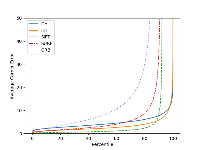
Figure 4: Sorted ACE for Ideal Conditions. SIFT gives superior performance for 90% of the data. However, in the final 8% of the dataset, SIFT has incredibly high error.

5.2 Noise

As shown in Table 3, the traditional feature-matching based methods are much more sensitive to noise than the CNN based methods. The SIFT and the SURF based homography estimators maintain a lower median ACE value than the CNN-based methods at $\eta=0.1$. However, when $\eta=0.3$, both the SIFT and the SURF based methods fail to find a sufficient number of feature correspondences for reliable homography estimation for over half the dataset. The two CNN method, though obviously affected by noise, remain much more robust over a significant fraction of the dataset.

Noise $\eta$	0.1	0.3	0.5
Method	Median ACE / OR
DH	13.60 / 0.01	21.73 / 0.01	28.49 / 0.03
HH	6.79 / 0.01	13.38 / 0.01	17.30 / 0.01
SIFT	2.33 / 0.18	NAN / 0.66	NAN / 0.94
SURF	5.42 / 0.17	NAN / 0.62	NAN / 0.93
ORB	12.20 / 0.16	26.50 / 0.34	53.12 / 0.52

Table 3: Median ACE and OR value in the presence of additive noise. HH has the best median ACE for “moderate” and “high” noise levels. “NAN” stands for “Not a Number”.

Fig. 5 shows the plots for the case of additive noise at the additive level of $\eta=0.3$. It is interesting to see while the traditional approach to homography estimation based on SIFT gives the best results on a small fraction of the dataset, it essentially fails to produce any usable results at all for a large part of the dataset. The other two traditional approaches do worse than the one based on SIFT. On the other hand, the two CNN based approaches work better for a much larger fraction of the overall dataset, although not matching the best (in terms of accuracy) that one can get with a SIFT based method.

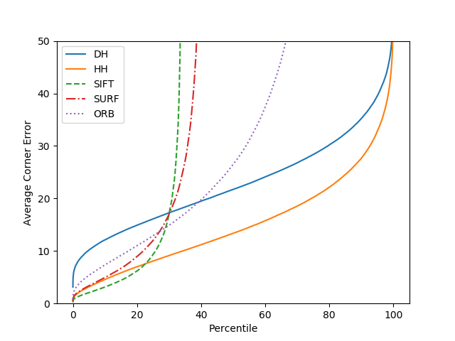
Figure 5: Sorted ACE for the noise level $\eta=0.3$. At a “moderate” level of noise, SIFT and SURF fail to give viable results for over 60% of the dataset. ORB is more robust, but not as robust as the CNNs.

5.3 Illumination

As shown in Table 4, the traditional feature-matching based methods have a better median ACE at “low” and “moderate” levels of shifts in illumination, but the HH based CNN homography estimator shows better Between the two CNNs, DH is impacted much more significantly by illumination shift. The discrepancy between the two CNNs could be explained by the fact that HH is based on a Siamese network, where two input patches are transformed by four convolutional layers before the features are combined. By contrast, DH stacks the input patches at the very beginning. The discrepancy in input patches, therefore, has a larger impact, as there is no opportunity for the network to isolate invariant features within each patch, independent of the other.

Illum $\lambda$	1.2	1.4	1.6
Method	Median ACE / OR
DH	23.08 / 0.01	26.45 / 0.01	28.38 / 0.01
HH	2.35 / 0.01	2.86 / 0.01	5.50 / 0.01
SIFT	0.95 / 0.10	1.35 / 0.17	10.70 / 0.47
SURF	3.41 / 0.12	5.65 / 0.26	NAN / 0.67
ORB	8.48 / 0.18	11.92 / 0.26	48.26 / 0.50

Table 4: Depicted are the ACE and OR for each method for the caes of illumination shifts. SIFT has a lower median ACE at “low” and “moderate” levels. At “high”, HH has a lower median ACE.

Fig. 6 shows how the performance varies across the dataset for illumination variance at $\lambda=1.6$. Under conditions of illumination variance, the traditional approaches to homography estimation work for only a small fraction of the dataset. Of the two CNN based methods, the DH solution does miserably across the board. While DH does not pass muster for this difficult case, what is achieved by the HH solution is indeed impressive.

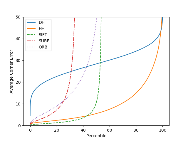
Figure 6: Sorted ACE for Illumination $\lambda=1.6$. HH has the lowest ACE for 56% of the dataset.

5.4 Occlusion

In comparison with additive noise and illumination variations, it is interesting to see that the traditional feature-matching based methods for homography estimation are not as sensitive to occlusions. As shown in Table 5, the SIFT based homography estimator retains the lowest median ACE at all three levels of occlusion while the two CNN based methods remain more consistent. This suggests that, as long as there is enough opportunity for distinct key points to be identified and matched, feature matching will experience little degradation.

Occlude $\alpha$	0.2	0.4	0.6
Method	Median ACE / OR
DH	4.74 / 0.01	6.99 / 0.01	11.23 / 0.01
HH	2.27 / 0.01	2.39 / 0.01	3.01 / 0.01
SIFT	0.91 / 0.10	0.99 / 0.13	1.29 / 0.21
SURF	3.52 / 0.12	4.85 / 0.20	14.94 / 0.41
ORB	9.75 / 0.21	22.04 / 0.39	96.03 / 0.74

Table 5: Values for the Median ACE and OR under occlusion. SIFT has the best median ACE for the different degrees of occlusion and experiences only a minor degradation of OR at $\alpha=0.6$.

Fig. 7 shows the performance plots for all five cases. SIFT does the best compared to the other two traditional methods. And, what is even more interesting, for a significant fraction of the images, SIFT even beats out the two CNN-based methods. But, as can be inferred from the rapid rise of the SIFT plot, it fails miserably at 79%. On the other hand, the two CNN based methods fail completely at a much smaller rate than SIFT.

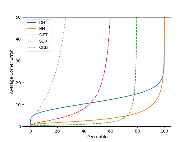
Figure 7: Sorted ACE values for the occlusion level of $\alpha=0.6$.

5.5 Color vs. Grayscale

As shown in Table 6, training the DH CNN with color inputs instead of grayscale inputs resulted in a slightly larger median error for the ACE metric.

Method	Median ACE	OR
DH Grayscale	3.97	0
DH Color	4.74	0

Table 6: Comparison of the DH network trained with grayscale images.

The performance plots are shown in Fig. 8. The graph for the grayscale case is consistently below the graph for color, implying that, with the same CNN architecture, the grayscale images result in slightly more accurate homographies than the color images.

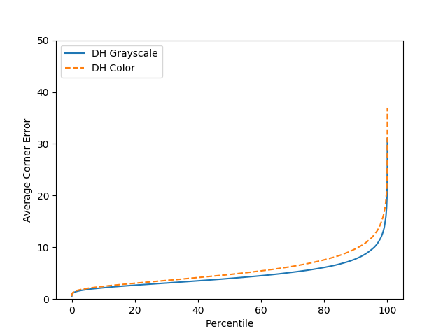
Figure 8: Performance plots for the color vs. grayscale comparison. Contrary to intuition, the results with color are slightly worse.

5.6 DH Trained with Noise-Corrupted Inputs

Table 7 presents the results obtained when the DH is trained with different amounts of noise added to the training dataset. The CNN based homography estimator achieved significantly superior performance when trained to the specific level of noise. However, this performance enhancement came with a small degradation in the performance for the noiseless case (Ideal). Additionally, training at a lower level of noise only slightly improved the performance at higher levels of noise.

Noise $\eta$	0	0.1	0.3	0.5
Method	Median ACE
DH	3.97	13.60	21.73	28.49
DH Noise 10	10.08	4.24	20.93	26.40
DH Noise 30	6.25	5.99	4.99	20.17
DH Noise 50	5.66	5.54	5.62	5.70

Table 7: Deep Image Homography Trained With Noise. The table shows the median ACE values for the case when the DH network is trained with different degrees of noise.

Shown in Fig. 9 are the percentile plots for the case when the three different DH networks, each trained with one of the three noisy input datasets as listed in Table 7), are tested on the same input-plus-noise data set corresponding to $\eta=0.5$. Since the red-dotted plot for the case “DH Noise 50” is the slowest rising graph in the figure, this again shows that one gets the best results when the level of noise at which the DH is trained matches the level of noise in the input images.

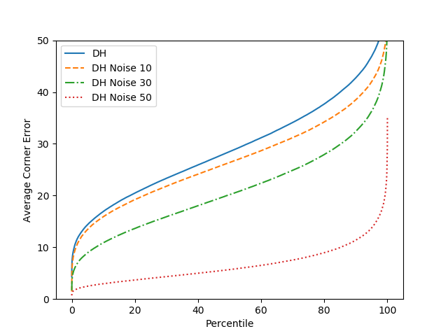
Figure 9: Sorted ACE values for the DH network that is trained to noise with the $\eta=0.5$ dataset. The CNN trained with the highest level of noise also performs the best under high noise conditions.

6 Conclusion

Under what we have referred to as the Ideal conditions and under conditions of low variance, feature matching based homography estimation (particularly SIFT) is still the most accurate method (per median ACE).

However, in conditions of moderate to heavy variance, especially with Gaussian noise, CNN-based homography estimation achieves a lower median ACE. Under these conditions, the feature matching based methods consistently suffered sensitivity to variance. The CNN-based homography estimators learned to be more robust even when the training was confined to ideal conditions.

Our experiments have also demonstrated that the robustness to noise for CNN-based homography estimators can be further improved by training with noisy data. Our experiments showed that the performance improved significantly at the specific level of noise with which the CNN trained. However, that improved performance comes at a slight degradation to accuracy in ideal conditions. There was only little improvement to performance in higher magnitudes of noise. Essentially, by training to a specific magnitude of noise, a “Goldilocks Zone” is created where that CNN performs best. More experiments need to be conducted to determine the ideal process for training in noise that optimizes performance across all potential magnitudes of noise.

CNN-based homography estimators produced more consistent results than the feature-matching based estimators in all conditions. While SIFT produced outputs with unacceptable errors on 8% of the Ideal conditions, the CNN based methods produced such outputs for less than one percent in any conditions. This is likely because CNNs can be trained to a specific range of homography values, unlike feature-matching. Many applications, such as real-time tracking for AR, might benefit in consistency over absolute error.

Explicitly including color channels at the input for training CNN based homography estimators did not produce significantly better results for CNN based methods. Despite the additional information provided by the different color channels, the CNN-based homography estimation actually performed slightly worse. However, it is possible that a more elaborate architecture would yield higher accuracies for the homographies estimated from color images. Additionally, given the redundancy between the RGB channels of a color image, such inputs might increase robustness against noise. More research is necessary to find the optimal architecture and training methods that best leverages the additional information available in color images.

The overall lesson learned from our research is that no one method for homography estimation can be treated as “universally superior” to all others. The environmental conditions and engineering constraints need to be deliberately considered when choosing the most appropriate technique in any application. While CNN-based homography estimators may not be as accurate as the best “hand-crafted” feature-based algorithms, they are more consistent and perform better in conditions of variance (noise, illumination shifts, and occlusions).

References

- [1] H. Bay, T. Tuytelaars, and L. Van Gool. SURF: Speeded Up Robust Features. In European conference on computer vision, pages 404–417. Springer, 2006.
- [2] G. Bradski. The OpenCV Library. Dr. Dobb’s Journal of Software Tools, 2000.
- [3] D. DeTone, T. Malisiewicz, and A. Rabinovich. Deep image homography estimation. CoRR, abs/1606.03798, 2016.
- [4] E. Dubrofsky. Homography estimation, 2009.
- [5] M. A. Fischler and R. C. Bolles. Random sample consensus: A paradigm for model fitting with applications to image analysis and automated cartography. Commun. ACM, 24(6):381–395, June 1981.
- [6] I. Goodfellow, J. Pouget-Abadie, M. Mirza, B. Xu, D. Warde-Farley, S. Ozair, A. Courville, and Y. Bengio. Generative adversarial nets. In Advances in neural information processing systems, pages 2672–2680, 2014.
- [7] X. Han, T. Leung, Y. Jia, R. Sukthankar, and A. C. Berg. Matchnet: Unifying feature and metric learning for patch-based matching. In Proceedings of the IEEE Conference on Computer Vision and Pattern Recognition, pages 3279–3286, 2015.
- [8] D. P. Kingma and J. Ba. Adam: A method for stochastic optimization. CoRR, abs/1412.6980, 2014.
- [9] I. Krasin, T. Duerig, N. Alldrin, V. Ferrari, S. Abu-El-Haija, A. Kuznetsova, H. Rom, J. Uijlings, S. Popov, S. Kamali, M. Malloci, J. Pont-Tuset, A. Veit, S. Belongie, V. Gomes, A. Gupta, C. Sun, G. Chechik, D. Cai, Z. Feng, D. Narayanan, and K. Murphy. Openimages: A public dataset for large-scale multi-label and multi-class image classification. Dataset available from https://storage.googleapis.com/openimages/web/index.html, 2017.
- [10] A. Kuznetsova, H. Rom, N. Alldrin, J. Uijlings, I. Krasin, J. Pont-Tuset, S. Kamali, S. Popov, M. Malloci, T. Duerig, and V. Ferrari. The open images dataset v4: Unified image classification, object detection, and visual relationship detection at scale. arXiv:1811.00982, 2018.
- [11] T.-Y. Lin, M. Maire, S. J. Belongie, L. D. Bourdev, R. B. Girshick, J. Hays, P. Perona, D. Ramanan, P. Dollár, and C. L. Zitnick. Microsoft COCO: Common objects in context. In ECCV, 2014.
- [12] H. Liu, G. Zhang, and H. Bao. Robust keyframe-based monocular slam for augmented reality. In 2016 IEEE International Symposium on Mixed and Augmented Reality (ISMAR), pages 1–10, Sep. 2016.
- [13] D. G. Lowe. Distinctive image features from scale-invariant keypoints. International journal of computer vision, 60(2):91–110, 2004.
- [14] T. Nguyen, S. W. Chen, S. S. Shivakumar, C. J. Taylor, and V. Kumar. Unsupervised deep homography: A fast and robust homography estimation model. CoRR, abs/1709.03966, 2017.
- [15] F. E. Nowruzi, R. Laganiere, and N. Japkowicz. Homography estimation from image pairs with hierarchical convolutional networks. In 2017 IEEE International Conference on Computer Vision Workshops (ICCVW), pages 904–911, Oct 2017.
- [16] A. Paszke, S. Gross, S. Chintala, G. Chanan, E. Yang, Z. DeVito, Z. Lin, A. Desmaison, L. Antiga, and A. Lerer. Automatic differentiation in PyTorch. In NIPS Autodiff Workshop, 2017.
- [17] E. Rublee, V. Rabaud, K. Konolige, and G. R. Bradski. ORB: An efficient alternative to SIFT or SURF. In ICCV, volume 11, page 2. Citeseer, 2011.
- [18] K. Simonyan and A. Zisserman. Very deep convolutional networks for large-scale image recognition. CoRR, abs/1409.1556, 2014.
- [19] E. Vincent and R. Laganière. Detecting planar homographies in an image pair. ISPA 2001. Proceedings of the 2nd International Symposium on Image and Signal Processing and Analysis. In conjunction with 23rd International Conference on Information Technology Interfaces (IEEE Cat., pages 182–187, 2001.