Generalized Centrality Aggregation and Exclusive Centrality

Abstract

There are several applications that benefit from a definition of centrality which is applicable to sets of vertices, rather than individual vertices. However, existing definitions might not be able to help us in answering several network analysis questions. In this paper, we study generalizing aggregation of centralities of individual vertices, to the centrality of the set consisting of these vertices. In particular, we propose exclusive betweenness centrality, defined as the number of shortest paths passing over exactly one of the vertices in the set, and discuss how this can be useful in determining the proper center of a network. We mathematically formulate the relationship between exclusive betweenness centrality and the existing notions of set centrality, and use this relation to present an exact algorithm for computing exclusive betweenness centrality. Since it is usually practically intractable to compute exact centrality scores for large real-world networks, we also present approximate algorithms for estimating exclusive betweenness centrality. In the end, we evaluate the empirical efficiency of exclusive betweenness centrality computation over several real-world networks. Moreover, we empirically study the correlations between exclusive betweenness centrality and the existing set centrality notions.

I Introduction

Centrality is a structural attribute of vertices in a network, used to determine the relative importance of a vertex or a set of vertices in the network. For example, it can be used to determine how influential a person is within a social network, or how well-used a road/intersection is within a road network. There are several measures of centrality in literature, including degree centrality defined as the number of links incident upon a vertex, closeness centrality, defined as the inverse of the sum of the distances between the vertex and all other vertices, and eigen-vector centrality wherein connections to high-scoring vertices contribute more to the centrality score of the vertex than equal connections to low-scoring vertices [5]. Another well-known centrality notion is betweenness centrality, defined as the number (or the ratio) of shortest paths from all vertices to all others that pass over the vertex. It first was introduced by Linton Freemana as a measure for quantifying the control of a human on the communication between other humans in a social network [20].

There are several applications that benefit from a definition of centrality which is applicable to sets of vertices rather than individual vertices [19]. Therefore in the literature, a few extensions of centrality notions to sets are introduced. When the centrality measure is betweenness centrality (which is the main concern of this paper), two already studied ways of extending vertex betweenness centrality to sets of vertices are:

• group betweenness centrality of a set, which is defined as the number of shortest paths that pass over at least one of the vertices in the set [19, 16], and

• co-betweenness centrality of a set, which is defined as the number of shortest paths that pass over all the vertices in the set [21, 9].

The authors of [21] showed that these two notions are related and developed a mathematical characterization of their relationship. These two notions of set centrality provide a measure for the importance or influence of a set vertices in a network. However, they provide only two specific cases of many possibilities for extending a centrality notion from vertices to the sets. Moreover, they might not be able to help us in answering network analysis questions such as: when should a center consisting of an individual vertex $v$ be extended to a center consisting of $v$ and another vertex $u$? Or, more generally, how someone can decide whether a set $A$ is a good enough center for a network $G$, or it should be extended to a larger set $A^{\prime}$, $A\subset A^{\prime}$, in order to form a better center for $G$? As we will discuss in more details in Section III, group betweenness centrality and co-betweenness centrality do not provide proper answers to the above mentioned questions.

In this paper, we study generalizing aggregation of centrality of individual vertices to the sets. In particular, we discuss that in several case, more the existing extensions of centrality notions, it is useful to have some other centrality extensions for the sets. Then we propose exclusive betweenness centrality, a novel extension of betweenness centrality to sets, defined as the number of shortest paths passing over exactly one of the vertices in the set. We discuss how this measure fulfills the conditions required for the centrality of a set, e.g., it says whether a set $A$ is a good center of the network or it should be extended to a larger set $A^{\prime}$. Then, We mathematically formulate the relationship between exclusive betweenness centrality and the existing notions of set centrality, and use this relation to present an exact algorithm for computing exclusive betweenness centrality. Then, since it is usually practically intractable to compute exact centrality scores in large real-world networks, we present approximate algorithms for estimating exclusive betweenness centrality. In particular, we present a general algorithm and discuss how it can be specialized to yield different source sampling, pair sampling and shortest path sampling algorithms. In the end, by conducting experiments over several real-world networks, we empirically evaluate our results. In our experiments, first we evaluate the running time of exact exclusive betweenness centrality computation over several real-world networks. Second, we empirically investigate the correlation between exclusive betweenness centrality and group betweenness centrality, and the correlation between exclusive betweenness centrality and co-betweenness centrality.

The rest of this paper is organized as follows. In Section II, preliminaries and definitions related to betweenness centrality are presented. In Section III, we motivate and introduce exclusive betweenness centrality and discuss its usefulness. In Section IV, we discuss the mathematical relationship between exclusive and co-betweenness centralities, and present several exact and approximate algorithms for computing/estimating exclusive betweenness centrality of a given set (or all subsets of the vertices). In Section V, we present our empirical results on exclusive betweenness centrality computation, as well as on the correlations between the set centrality notions. In Section VI, we have a brief overview on related work. Finally, in Section VII, the paper is concluded.

II Preliminaries

In this section, we present definitions and notations widely used in the paper. We assume that the reader is familiar with basic concepts in graph theory. Throughout the paper, $G$ refers to a graph (network). For simplicity, we assume that $G$ is a connected and loop-free graph without multi-edges. $V(G)$ and $E(G)$ refer to the set of vertices and the set of edges of $G$, respectively. Furthermore, we use $n$ to point to $|V(G)|$, and $m$ points to $|E(G)|$. For an edge $e=(u,v)\in E(G)$, $u$ and $v$ are the two end-points of $e$.

A shortest path (also called a geodesic path) between two vertices $u,v\in V(G)$ is a path whose size is minimum, among all paths between $u$ and $v$. For two vertices $u,v\in V(G)$, we use $d_{G}(u,v)$, or $d(u,v)$ when $G$ is clear from the context, to denote the size (the number of edges) of a shortest path connecting $u$ to $v$. By definition, $d_{G}(u,v)=0$ and $d_{G}(u,v)=d_{G}(v,u)$.

For $s,t\in V(G)$, $\sigma_{st}$ denotes the number of shortest paths between $s$ and $t$; and $\sigma_{st}(v)$ denotes the number of shortest paths between $s$ and $t$ that also pass through $v$. We have:

$$\sigma_{s}(v)=\sum_{t\in V(G)\setminus\{s,v\}}\sigma_{st}(v).$$

Betweenness centrality of a vertex $v$ is defined as:

$$\mathcal{B}(v)=\sum_{s,t\in V(G)\setminus\{v\}}\sigma_{st}(v).$$ (1)

A notion which is widely used for counting the number of shortest paths in a graph is the directed acyclic graph (DAG) containing all shortest paths starting from a vertex $s$ (see e.g. [7]). In this paper, we refer to it as the shortest-path-DAG, or SPD for short, rooted at $s$. For every vertex $s$ in a graph $G$, the SPD rooted at $s$ is unique, and it can be computed in $O(m)$ time for unweighted graphs and in $O(m+n\log n)$ time for weighted graphs with positive weights [7].

The dependency score of a vertex $s\in V(G)$ on a vertex $x\in V(G)\setminus\{s\}$ is defined as:

$$\delta_{s\bullet}(v)=\sum_{t\in V(G)\setminus\{v,s\}}\sigma_{st}(v).$$ (2)

We have :

$$\mathcal{B}(v)=\sum_{s\in V(\mathbf{G})\setminus\{v\}}\delta_{s\bullet}(v)$$ (3)

III Exclusive centrality

In the literature, there exist algorithms that extend a centrality notion defined for a single vertex to a set of vertices [19, 21, 9, 16]. This is done for different centrality notions, and the usefulness of such extensions has been studied in different applications. We refer to such extensions, in a general form, as the set aggregation of the centrality notion. Hence, an aggregation function is used to aggregate centrality scores of individual vertices in the set and yield the centrality score of the whole set. However, in the literature only some specific aggregation functions have been introduced and used. Foe example, in group betweenness centrality, the aggregation function is defined as counting the number (or the ratio) of shortest paths that pass over at least one of the vertices in the set [19, 16]. in co-betweenness centrality, the aggregation function is defined as counting the number (or the ratio) of shortest paths that pass over all the vertices in the set [21, 9]. These two extensions are only two specific forms, out of many other possibilities, that are introduced and used in the literature.

In this paper, we go beyond these two specific cases, formulate the general form of aggregation, and motivate and discuss a new case of set aggregation. Let $A\subset V(G)$ be the set for which we want to define the centrality notion. Given a centrality notion $\mathcal{C}$ and an aggregation function $Agg$ defined over the set of vertices in $A$, the $\mathcal{C}$ centrality of $A$ is defined as follows:

$$\mathcal{C}_{Agg}(A)=Agg(\mathcal{C}(v):v\in A)$$ (4)

In [19], the authors suggested considering centrality of a set of vertices as the number (or the ratio) of shortest paths that pass through at least one of the vertices in the set and introduce the group betweenness centrality. More formally:

$$\mathcal{GB}(A)=\sum_{s,t\notin A:s\neq t}\sigma^{*}_{st}(A),$$ (5)

where $\sigma^{*}_{st}(A)$ refers to the number of shortest paths between $s$ and $t$ that pass through at least one of the vertices in $A$. The other natural extension is co-betweenness centrality, which is presented by Kolaczyk et.al. [21] as the following:

$$\mathcal{CB}(A)=\sum_{s,t\notin A:s\neq t}\hat{\sigma}_{st}(A),$$ (6)

where $\hat{\sigma}_{st}(A)$ is defined as the number of shortest paths between $s$ and $t$ that pass through all the vertices in $A$, and

$$\hat{\sigma}_{s}(A)=\sum_{t\in V(G)\setminus\{s\}\setminus A}\hat{\sigma}_{st}(A).$$

In Equation 5, for every two subsets $A$ and $A^{\prime}$ of the vertices such that $A\subset A^{\prime}$, we have: $\mathcal{GB}(A)\leq\mathcal{GB}(A^{\prime})$, i.e., by adding a new vertex to a set $A$, its group betweenness centrality increases or at least it does not change. We may refer to this property of group betweenness centrality as the monotonicity property. This property makes it difficult to use group betweenness centrality for answering questions such as the following:

Given a set $A\subset V(G)$ and a vertex $v\in V(G)\setminus A$, between $A$ and $A\cup\{v\}$ which one is a better center for $G$?

The reason is that on the one hand $A\cup\{v\}$ has always a non-less group betweenness centrality than $A$. On the other hand, however it is always desirable to keep the center of a network as small as possible. So in this sense, sometimes we may prefer $A$ to $A\cup\{v\}$ if adding the new vertex $v$ increases the centrality/importance of the set just a little (if not at all). More than the applicability aspects, the computation cost may also encourage us to choose small sets, as computing group betweenness centrality of a set usually increases by increasing its size.

An attempt to find a good set of vertices as the center of a network was finding a prominent set [25]. A prominent set is a set of minimum size, such that every shortest path in the network passes through at least one of the vertices in the set. However, this notion of prominent groups has shortcomings. First, the problem of finding a prominent group is a simple reduction of the minimal vertex cover problem [25] and hence, it is an NP-hard problem. Second, the size of a prominent group can be large, as it tries to control all the flows (which are done through shortest paths) in the network.

To answer the above-mentioned question and alleviate the discussed challenges, we present a new set centrality aggregation function, that compares/ranks a set against its subsets. In the proposed measure, called exclusive betweenness centrality and denoted with $\mathcal{XB}$, the following observations are considered:

1. Let $A$ be a subset of $V(G)$, $v$ be a vertex in $G$, $S$ be the set of all shortest paths in $G$, $S(v)$ be the set of shortest paths in $G$ that pass through $v$ and $S(A)$ be the set of shortest paths in $G$ that pass through at least one of members of $A$. For two vertices $v_{1},v_{2}\in V(G)\setminus A$, if $|S(\{v_{1}\}\cup A)|>|S(\{v_{2}\}\cup A)|$, the exclusive betweenness centrality of $\{v_{1}\}\cup A$ should be greater than the exclusive betweenness centrality of $\{v_{2}\}\cup A$.

2. If a considerable number of (or most of) those shortest paths of $G$ that pass over $v$ also pass over the members of $A$, exclusive betweenness centrality of $A$ should be greater than exclusive betweenness centrality of $A\cup\{v\}$. The reason is that while computing centrality of $A\cup\{v\}$ is more time consuming than computing centrality of $A$, $A\cup\{v\}$ does not control flows of the network (much) more than $A$. This means finding larger sets as the centers of the network must be done only when they considerably increase the control over the flows in the network (i.e., they have a considerably larger centrality score than their proper subsets).

The first observation defines a property desirable when two different vertices $v_{1}$ and $v_{2}$ are added to the set. The second observation defines a property desirable when a new vertex is added to the set, compared to the case wherein the new vertex is not added. In the following, first in Definition 1 we present the definition of exclusive betweenness centrality of a set. Then, we discuss that it satisfies the two above-mentioned properties.

Definition 1.

Let $A=\{v_{1}\ldots v_{k}\}$ be a set of vertices. The exclusive betweenness centrality of $A$ is defined as follows:

$$\mathcal{XB}(\{v_{1}\ldots v_{k}\})=|S(v_{1})\mathbin{\oplus}\ldots\mathbin{\oplus}S(v_{k})|$$ (7)

where $\mathbin{\oplus}$ of two sets $S_{1}$ and $S_{2}$ is their exclusive or, i.e., $S_{1}\mathbin{\oplus}S_{2}=(S_{1}\setminus S_{2})\cup(S_{2}\setminus S_{1})$, and $S(v)$ is the set of shortest paths that pass through vertex $v$.

As an example of exclusive betweenness centrality, consider Figure 1, wherein Figure 1(a) shows a graph $G$ and Figure 1(b) shows the shortest path DAG rooted at the vertex $s=1$. Assume that the set $A$ consists of vertices $2,6,7$. Those shortest paths that start from vertex $1$ and pass over exactly one of the members of $A$ (hence, contribute to the exclusive betweenness centrality of $A$) are as follows: $1\rightarrow 2\rightarrow 4$, $1\rightarrow 2\rightarrow 5$, $1\rightarrow 2\rightarrow 5\rightarrow 8$, $1\rightarrow 2\rightarrow 5\rightarrow 8\rightarrow 9$, $1\rightarrow 3\rightarrow 5\rightarrow 7\rightarrow 9$, $1\rightarrow 3\rightarrow 6\rightarrow 8$, and $1\rightarrow 3\rightarrow 6\rightarrow 8\rightarrow 9$. Therefore, exclusive betweenness centrality of $A$ is $7$.

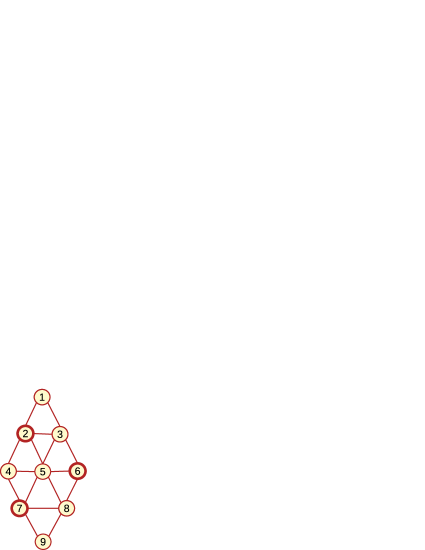
(a) A graph $G$

(b) The shortest path DAG rooted at vertex $1$.

Figure 1: An example of exclusive betweenness centrality. Exclusive betweenness centrality of $A=\{2,6,7\}$ is $7$.

The first observation mentioned above says that if the new vertex brings more new shortest paths controlled by the set, its union with the set must have a larger centrality score. Therefore, for any two vertices $v_{1}$ and $v_{2}$ and set $A$ of vertices, we may express it as follows:

if

$$\left|\left(S(v_{1})\setminus S(A)\right)\cup\left(S(A)\setminus S(v_{1})\right)\right|>\newline$$

$$\left|\left(S(v_{2})\setminus S(A)\right)\cup\left(S(A)\setminus S(v_{2})\right)\right|$$

then

$$\mathcal{XB}(A\cup\{v_{1}\})>\mathcal{XB}(A\cup\{v_{2}\})$$ (8)

It is easy to see that the definition of $\mathcal{XB}$ presented in Definition 1 satisfies this property.

For the second observation, we need to define a threshold for $|S(A\cup\{v\})\setminus S(A)|$ and as a result, for $|S(v)\setminus S(A)|$. We may define this threshold as the following:

$$|S(v)\setminus S(A)|\geq|S(A\cap\{v\})|.$$ (9)

If the threshold of Equation 9 holds, the number of shortest paths controlled by $A\cup\{v\}$ will be greater than or equal to the number of shortest paths controlled by $A$. More precisely, using some simple tricks from relational algebra, Equation 9 yields:

$$|S(v)\setminus S(A)\cup S(A)\setminus S(v)|\geq|S(A)|,$$ (10)

which yields that

$$\mathcal{XB}(A\cup\{v\})\geq\mathcal{XB}(A).$$ (11)

This means if we use exclusive betweenness centrality, as presented in Definition 7, the larger set $A\cup\{v\}$ is preferred to the smaller set $A$, if the the threshold of Equation 9 holds, i.e., if the number of shortest paths controlled by $v$ but not by $A$ is greater than (or equal to) the number of shortest paths controlled by both $A$ and $v$.

IV Algorithmic aspects

In this section, we investigate the relationship between exclusive betweenness centrality and co-betweenness centrality, and exploit this relationship to present an exact algorithm for computing exclusive betweenness centrality. We also discuss some approximation techniques for estimating exclusive betweenness centrality.

IV-A Relation to other centrality notions

Kolaczyk et.al. [21] showed that group betweenness centrality of a set $A$ can be expressed in terms of co-betweenness centrality, as follows:

$$\mathcal{GB}(A)=\sum_{j=1}^{|A|}(-1)^{j-1}\sum_{\mathbf{i}_{j}\subseteq A}\mathcal{CC}_{A}(\mathbf{i}_{j}),$$ (12)

where $\mathbf{i}_{j}$ is a subset of size $j$ of $A$ and $\mathcal{CC}_{A}(\mathbf{i}_{j})$ is the $j$-th order co-betweenness of $\mathbf{i}_{j}$ with respect to $A$, defined as follows:

$$\mathcal{CC}_{A}(\mathbf{i}_{j})=\sum_{s,t\notin A:s\neq t}\hat{\sigma}_{st}(\mathbf{i}_{j}).$$ (13)

In a similar way, it can be shown that exclusive betweenness centrality can be re-written in terms of co-betweenness centrality of subsets of $A$ as follows:

$$\mathcal{XB}(A)=\sum_{j=1}^{|A|}j(-1)^{j-1}\sum_{\mathbf{i}_{j}\subseteq A}\mathcal{CC}_{A}(\mathbf{i}_{j})$$ (14)

Note that for the special case of $|\mathbf{i}_{j}|=1$, $\mathcal{CC}_{A}(\mathbf{i}_{j})$ gives betweenness centrality of $\mathbf{i}_{j}$, with a small difference that source and target vertices of shortest paths can not be in $A$. We refer to this value as $\mathcal{B}_{A}(\mathbf{i}_{j})$. As a simple case, consider the situation wherein the set $A$ consists of two vertices $v_{1}$ and $v_{2}$. Using Equation 14, exclusive betweenness centrality of $\{v_{1},v_{2}\}$ can be written as follows:

$$\mathcal{XB}(\{v_{1},v_{2}\})=$$

$$\mathcal{B}_{\{v_{1},v_{2}\}}(\{v_{1}\})+\mathcal{B}_{\{v_{1},v_{2}\}}(\{v_{2}\})-2\mathcal{CC}_{\{v_{1},v_{2}\}}(\{v_{1},v_{2}\})$$ .

IV-B Computing exclusive betweenness centrality

A naive approach to compute exclusive betweenness centrality of a given set is to enumerate all shortest paths of the graph one-by-one, and check which one passes over exactly one of the vertices in $A$. Since the number of all shortest paths of the graph (and the number of shortest paths that pass over exactly one of the vertices in $A$) is exponential in the worst case (in terms of $n$), this approach gives a worst case exponential time algorithm.

A more practical approach is to use the following inclusion-exclusion relationship:

$$\mathcal{XB}(A) =\sum_{v_{i}\in A}\mathcal{B}_{A}(v_{i})-2\sum_{\text{subsets }\{u,v\}\text{ of size 2 of }A}\mathcal{CC}_{A}(\{u,v\})$$

$$+3\sum_{\text{subsets }\{u,v,w\}\text{ of size 3 of }A}\mathcal{CC}_{A}(\{u,v,w\})-\ldots$$ (15)

In this approach, exclusive betweenness centrality of $A$ is computed based on betweenness centrality of the individual vertices in $A$ and co-betweenness centrality of the (larger) subsets of $A$. While co-betweenness centrality of each subset of $A$ with an odd size contributes positively, the contribution of each subset whose size is even is negative. Using the method described in [9], co-betweenness centrality of a set of vertices can be computed efficiently (in a low degree polynomial time, in terms of $m$ and $n$). Overall, if the size of $A$ is considered as a constant, since in this approach a constant number of betweenness/co-betweenness scores will be computed, its time complexity will be polynomial in terms of $n$ and $m$ ($O(nm)$ for unweighted graphs and $O(nm+n^{2}\log n)$ for weighted graphs with positive weights). Obviously, since the number of subsets of $A$ is exponential, time complexity of this approach is exponential in terms of $|A|$.

IV-C Approximate algorithms

For large real-world networks consisting of thousands or millions of vertices, exact algorithms for computing centrality scores are usually intractable in practice. Therefore, in recent years several approximate algorithms have been developed for them. An extensive study of approximate algorithms for group betweenness centrality can be found in [16]. In the following, we investigate how these techniques can be revised to compute exclusive betweenness centrality.

Algorithm 1 High level pseudo code of the algorithm of estimating exclusive betweenness centrality.

1:  ApproximateExclusiveBetweenness

2:  Input. A graph $G$, a non-empty set $A\subset V(G)$, and the number of samples $T$.

3:  Output. Exclusive betweenness centrality of $A$.

4:  $\beta\leftarrow 0$.

5:  Compute probabilities $p_{ij}$, for each pair $(i,j)\in\mathcal{N}$.

6:  for all $t=1$ to $T$  do

7:     Select a pair $(i,j)\in\mathcal{N}$ with probability $p_{ij}$.

8:     Let $\Pi_{ij}$ be the set of all shortest paths between $i$ and $j$. Compute Probabilities $q_{k}$, for each $\pi_{k}\in\Pi_{ij}$.

9:     Select a shortest path $\pi_{k}\in\Pi_{ij}$, with probability $q_{k}$.

10:     if exactly one of the members of $A$ are on $\pi_{k}$ then

11:        $\beta_{t}\leftarrow\frac{1}{p_{ij}\cdot q_{k}}$.

12:        $\beta\leftarrow\beta+\frac{\beta_{t}}{T}$.

13:     end if

14:  end for

15:  return  $\beta$.

Algorithm 1 shows the high level pseudo code of a general algorithm for estimating exclusive betweenness centrality. It is similar to the general algorithm we presented in [16] for group betweenness centrality. The key difference is that when a shortest path is sampled, in Algorithm 1 it is checked whether exactly one of the vertices of $A$ are on the shortest path. In estimating group betweenness centrality [16], it is checked whether at least one of the vertices of $A$ are on the shortest path. Let $\mathcal{N}$ be the set of pairs in $\left(V(G)\setminus A\right)\times\left(V(G)\setminus A\right)$. The input parameters of the algorithm are the graph $G$, the set $A$ for which we want to estimate exclusive betweenness centrality, and the number of samples (iterations) $T$. First, Algorithm 1 computes probabilities $p_{ij}$, for each pair $(i,j)\in\mathcal{N}$. The probabilities $p_{ij}$ must satisfy the following conditions: i) for each $(i,j)\in\mathcal{N}$, $p_{ij}>0$, and ii) $\sum_{(i,j)\in\mathcal{N}}p_{ij}=1$. Then, at each iteration $t$ of the loop in Lines 6-14 of Algorithm 1:

• a pair $(i,j)\in\mathcal{N}$ is selected with probability $p_{ij}$,

• let $\Pi_{ij}$ be the set of all shortest paths between $i$ and $j$. Probabilities $q_{k}$ are computed, for each shortest path $\pi_{k}\in\Pi_{ij}$,

• a shortest path $\pi_{k}$ from $i$ to $j$ is selected with probability $q_{k}$,

• if exactly one of the members of $A$ are on $\pi_{k}$, $\beta_{t}$, the estimation of $\mathcal{XB}(A)$ at iteration $t$, is defined as

  $$\frac{1}{p_{ij}\cdot q_{k}}.$$

  Otherwise, it is defined as $0$.

The average of exclusive betweenness scores estimated at different iterations is returned as the final estimation of the exclusive betweenness centrality of $A$. In a way similar to Lemma 1 of [16], it can be shown that $\beta$ yields an unbiased estimation of exclusive betweenness centrality of $A$, i.e., the expected value of $\beta$ is equal to the exclusive betweenness centrality of $A$.

Note that while Algorithm 1 estimates exclusive betweenness centrality of a given set $A$, it can be simply revised to estimates exclusive betweenness centrality of all (non-empty and proper) subsets of the vertices of $G$. To do so, at each iteration $t$ and after sampling the shortest path $\pi_{k}$, the exclusive betweenness score of any (non-empty) subset of the vertices of $G$ that satisfies both of the following conditions:

• its exactly one member is an internal vertex of $\pi_{k}$, and

• none of its members are either the source or the target of $\pi_{k}$,

is estimated as

$$\frac{1}{p_{ij}\cdot q_{k}}$$

and any other subset of $V(G)$ as $0$. The final estimation of the exclusive betweenness centrality of each subset is the average of its estimated exclusive betweenness scores, at different iterations. The key difference between this case and the case of estimating group betweenness centrality of all subsets of the vertices is as follows: for group betweenness centrality, as mentioned in [16], at each iteration $t$ and after sampling the shortest path $\pi_{k}$, group betweenness score of any (non-empty) subset of the vertices of $G$ whose at least one member is an internal vertex of $\pi_{k}$, is estimated as

$$\frac{1}{p_{ij}\cdot q_{k}},$$

and any other subset of $V(G)$ as $0$.

In the following, we present some specific forms of the above mentioned general algorithm.

• In a source vertex sampling algorithm, at each iteration, first a source vertex $i$ is sampled with probability $p_{i}$. Then, the number of shortest paths that start from $i$ and pass over exactly one of the members of $A$, is counted. Then, this number is divided by $p_{i}$ to yield the estimation of the exclusive betweenness centrality of $A$ at the current iteration. In the end, the final estimation is the average of estimations of different iterations. In a special case of this algorithm, called uniform source vertex sampling algorithm, for each vertex $i\in V(G)\setminus A$, $p_{i}$ is defined as

  $$\frac{1}{|V(G)\setminus A|};$$

  and for each vertex $i\in A$, it is defined as $0$.

• In a pair sampling algorithm, at each iteration, first a source vertex $i$ and a target vertex $j$ (a pair of vertices $i,j$) are sampled with probability $p_{ij}$. Then, the number of shortest paths that start from $i$, pass over exactly one of the members of $A$ and end to $j$ is counted. Then, this number is divided by $p_{ij}$ to yield the estimation of the exclusive betweenness centrality of $A$ at the current iteration. In the end, the final estimation is the average of estimations of different iterations. In a special form of this algorithm, called uniform pair sampling algorithm, for each pair of vertices $i,j\in V(G)\setminus A\times\in V(G)\setminus A$ ($i\neq j$), $p_{ij}$ is defined as

  $$\frac{1}{(|V(G)\setminus A|)(|V(G)\setminus A|-1)}$$

  and for any other pair, it is defined as $0$.

• In a form of shortest path sampling algorithm, at each iteration, first a pair of vertices $i,j\in(V(G)\setminus A)\times(V(G)\setminus A)$ so that $i\neq j$ are sampled uniformly at random. Then, one of the shortest paths from $i$ to $j$ is sampled uniformly at random. Then, it is checked whether exactly one of the vertices in $A$ is an internal vertex of the sampled path. The number such occurrences during different iterations is counted. In the end, this count is scaled to give an unbiased estimation of the exclusive betweenness centrality of $A$.

V Experimental results

In this section, we empirically analyze exclusive betweenness centrality. First, we evaluate running time of computing exclusive betweenness centrality over a number of real-world networks. Then, we investigate the correlation between exclusive betweenness centrality and the other centrality notions of sets, such as group betweenness centrality and co-betweenness centrality. The experiments are done on one core of a single AMD Processor with 4 GB main memory.

V-A Empirical evaluation of exclusive betweenness centrality computation

We evaluate the empirical efficiency of the exact algorithm of computing exclusive betweenness centrality, discussed in Section IV. We test the algorithm over six real-world datasets. Table I summarizes specifications of the datasets. Figure 2(f) presents the running times (for different set sizes). Over each dataset, we considered different set sizes varying from $2$ to $5$. For each set size $k$, we select $50$ random subsets of the vertices of size $k$, and compute their exact exclusive betweenness scores. In the end, for each set size, we report in Figure 2(f) the running time of the set that takes the longest time. As can be seen in the figure, by increasing the set size, running time gradually increases. The reason is that as discussed in Section IV, by increasing the set size more co-betweenness centralities are required to be computed. This increases the run time of computing exclusive betweenness centrality. This is unlike the run time of computing co-betweenness centrality which as discussed in [9], usually decreases by increasing the size of the set.

TABLE I: Summary of real-world networks.

Dataset	# vertices	# edges	maximum degree	URL
jazz[26]	198	2.7K	100	http://networkrepository.com/jazz.php
bwm200 [26]	200	596	6	http://networkrepository.com/bwm200.php
can_187 [26]	187	652	9	http://networkrepository.com/can-187.php
can_256 [26]	256	1.3K	82	http://networkrepository.com/can-256.php
ca-netscience [26, 23]	379	914	34	http://networkrepository.com/ca-netscience.php
GD00_c [26]	638	1K	58	http://networkrepository.com/GD00-c.php

(a) bwm200

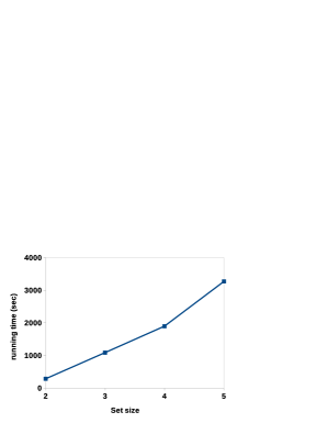
(b) can_187

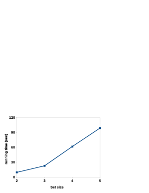
(c) can_256

(d) ca-netscience

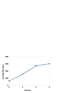
(e) GD00_c

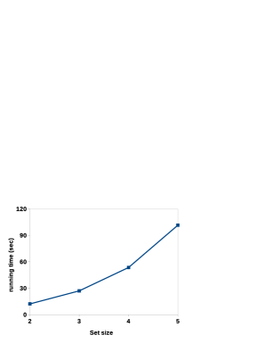
(f) jazz

Figure 2: Running time of the exclusive betweenness centrality computation algorithm over different datasets.

V-B Correlation with other set centrality notions

In this section, we investigate the correlation between exclusive betweenness centrality and group betweenness centrality and co-betweenness centrality. We examine the centrality notions on the well-known Zachary karate club network [29]. Zachary collected this dataset from the members of a university karate club. In this undirected network, each vertex represents a member of the club, and each edge represents a relationship between two members of the club. It has $34$ vertices, $78$ edges, its maximum degree $17$, and its diameter is and $5$. This network is depicted in Figure 3.

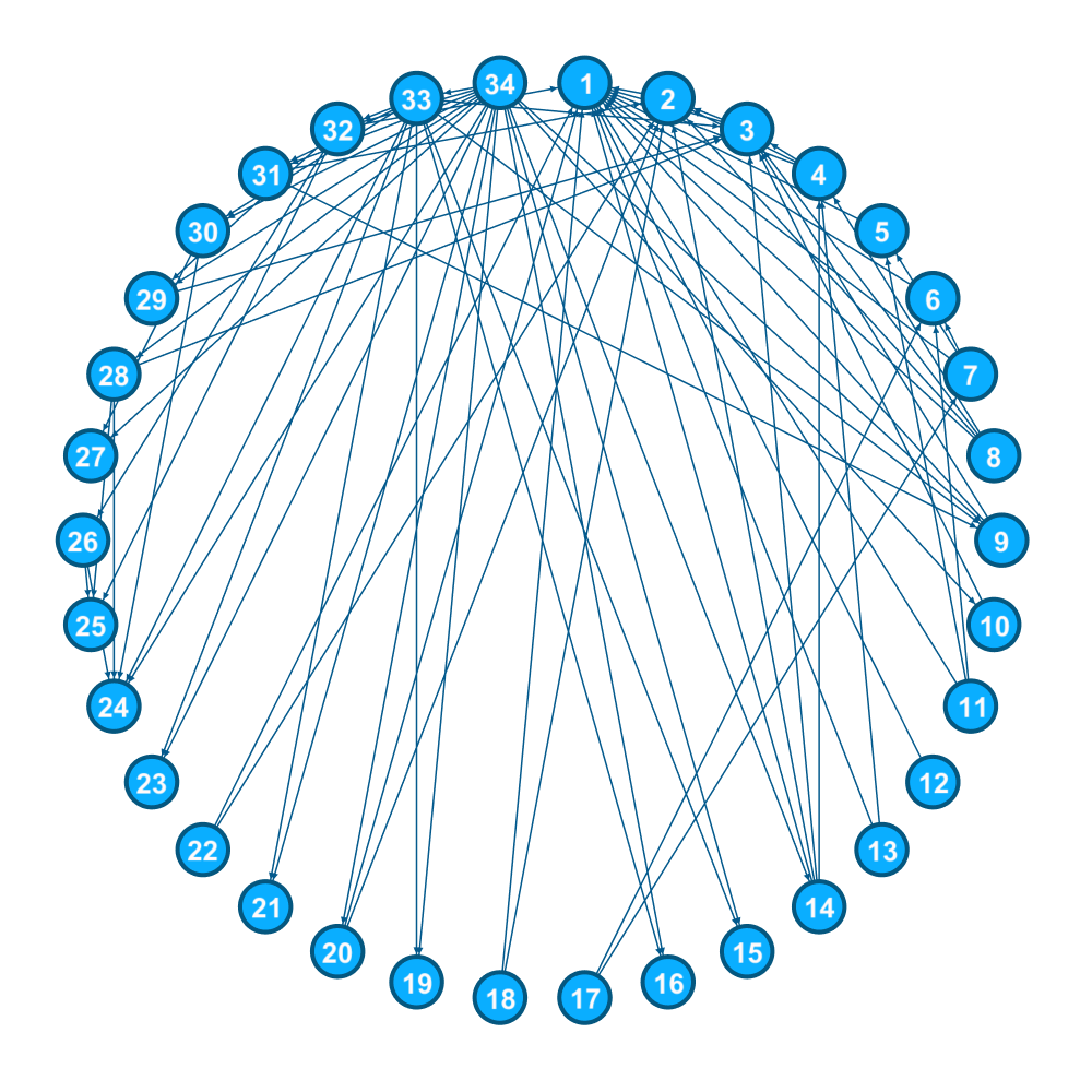
Figure 3: The Zachary karate club network. Source: Wikipedia

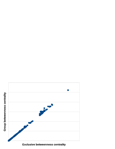
(a) The correlation between exclusive and group betweenness centralities.

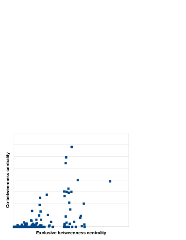
(b) The correlation between exclusive and co-betweenness centralities.

Figure 4: Correlations between exclusive betweenness centrality and the other set betweenness centralities.

Figure 4 represents the correlations, wherein the centrality values of all the sets of size $2$ are examined. As can be seen in the figure, there is almost a linear correlation between exclusive betweenness centrality and group betweenness centrality, so that sets with large group betweenness centrality have also a large exclusive betweenness centrality, and vice versa. However, the correlation between exclusive betweenness centrality and co-betweenness centrality is not direct and regular, as having a high exclusive betweenness score does not always imply a high co-betweenness centrality.

VI Related Work

Centrality measures are important and essential tools for analyzing social and information networks. some of widely used indices for centrality are betweenness centrality [20], closeness centrality [13], degree centrality [27], eigenvector centrality [5] and PageRank [1]. Betweenness centrality, which is widely used as a precise estimation of the information flow controlled by a vertex in social and information networks, assumes that information flow is done through shortest paths [28]. Barthelemy [4] showed that many scale-free networks [3, 8, 11] have a power-law distribution of betweenness Centrality. Brandes [7] introduced a new algorithm for computing betweenness centrality of a vertex, which is performed in $O(nm)$ time and $O(nm+n^{2}\log n)$ time for unweighted networks and (positively) weighted networks, respectively. In recent years several exact and approximate algorithms have been proposed to improve the efficiency of betweenness centrality computation [10, 15, 14, 12, 17].

Everett and Borgatti [19] defined group betweenness centrality as a natural extension of betweenness centrality for sets of vertices. The authors of [16] provided an extensive comparison of different group betweenness centrality estimation algorithm. They also presented an extension of distance-based sampling for group betweenness centrality. The other natural extension of betweenness centrality is co-betweenness centrality. Co-betweenness centrality is defined as the number of shortest paths passing through all vertices in the set [21]. The authors of [21] proposed an algorithm for individual co-betweenness centrality computation, that works only for sets of size $2$ and its time complexity is $O(n^{3})$. Chehreghani [9] presented algorithms for co-betweenness centrality computation of a set of an arbitrary size, and showed that by increasing the size of the set, its co-betweenness centrality can be computed more efficiently. Time complexity of these algorithms is $O(nm+n^{2}\log n)$ or less.

The authors of [18] presented the Routing Betweenness Centrality (RBC) index and proposed algorithms for computing RBC of individual vertices and algorithms for computing group RBC of a given set (or sequence) of vertices. Ballester et.al. [2] discussed the importance of finding the key group in a criminal network. Borgatti [6] discussed that the Key Player Problem (KPP) is strongly related to the cohesion of a network. He introduced two problems: KPP-Pos and KPP-Neg. He showed that the solution of KPP-Pos is a group maximally connected to all other vertices in a graph and the solution of KPP-Neg is a group maximally disrupting the network.

VII Conclusion

In this paper, we suggested generalizing the function of aggregating the centralities of the vertices of a set, to obtain the centrality of the whole set. As a particular case, we studied exclusive (betweenness) centrality, wherein the number of shortest paths that pass over exactly one of the vertices in the set, is counted. We also presented exact and approximate algorithms for computing exclusive betweenness centrality, efficiently. By conducting extensive experiments, first we evaluated the empirical efficiency of exclusive betweenness centrality computation. Then, we investigated the correlations between exclusive betweenness centrality and the other set centrality notions.

References

- [1] Arvind Arasu, Jasmine Novak, Andrew Tomkins, and John Tomlin. PageRank computation and the structure of the Web: Experiments and algorithms. In Proceedings of the Eleventh International World Wide, 2002.
- [2] Coralio Ballester, Antoni Calvó-Armengol, and Yves Zenou. Who’s who in networks. wanted: The key player. Econometrica, 74:1403 – 1417, 09 2006.
- [3] Albert-László Barabási and Réka Albert. Emergence of scaling in random networks. Science, 286(5439):509–512, 1999.
- [4] M Barthelemy. Betweenness Centrality in Large Complex Networks. Eur. Phys. J. B, 38(cond-mat/0309436):163. 6 p, Sep 2003.
- [5] Phillip Bonacich and Paulette Lloyd. Eigenvector-like measures of centrality for asymmetric relations. Social Networks, 23(3):191–201, July 2001.
- [6] Stephen P. Borgatti. Identifying sets of key players in a social network. 12(1):21–34, April 2006.
- [7] Ulrik Brandes. A Faster Algorithm for Betweenness Centrality. volume 25, pages 163–177, 2001.
- [8] Morteza Haghir Chehreghani and Mostafa Haghir Chehreghani. Modeling transitivity in complex networks. In Alexander T. Ihler and Dominik Janzing, editors, Proceedings of the Thirty-Second Conference on Uncertainty in Artificial Intelligence, UAI 2016, June 25-29, 2016, New York City, NY, USA. AUAI Press, 2016.
- [9] Mostafa Haghir Chehreghani. Effective co-betweenness centrality computation. In Ben Carterette, Fernando Diaz, Carlos Castillo, and Donald Metzler, editors, Seventh ACM International Conference on Web Search and Data Mining, WSDM 2014, New York, NY, USA, February 24-28, 2014, pages 423–432. ACM, 2014.
- [10] Mostafa Haghir Chehreghani. An efficient algorithm for approximate betweenness centrality computation. Comput. J., 57(9):1371–1382, 2014.
- [11] Mostafa Haghir Chehreghani and Talel Abdessalem. Upper and lower bounds for the q-entropy of network models with application to network model selection. Inf. Process. Lett., 119:1–8, 2017.
- [12] Mostafa Haghir Chehreghani, Talel Abdessalem, and Albert Bifet. Metropolis-hastings algorithms for estimating betweenness centrality. In Advances in Database Technology - 22nd International Conference on Extending Database Technology, EDBT 2019, Lisbon, Portugal, March 26-29, 2019, pages 686–689. OpenProceedings.org, 2019.
- [13] Mostafa Haghir Chehreghani, Albert Bifet, and Talel Abdessalem. Discriminative distance-based network indices with application to link prediction. Comput. J., 61(7):998–1014, 2018.
- [14] Mostafa Haghir Chehreghani, Albert Bifet, and Talel Abdessalem. Dybed: An efficient algorithm for updating betweenness centrality in directed dynamic graphs. In IEEE International Conference on Big Data, Big Data 2018, Seattle, WA, USA, December 10-13, 2018, pages 2114–2123. IEEE, 2018.
- [15] Mostafa Haghir Chehreghani, Albert Bifet, and Talel Abdessalem. Efficient exact and approximate algorithms for computing betweenness centrality in directed graphs. In Advances in Knowledge Discovery and Data Mining - 22nd Pacific-Asia Conference, PAKDD 2018, Melbourne, VIC, Australia, June 3-6, 2018, Proceedings, Part III, volume 10939 of Lecture Notes in Computer Science, pages 752–764. Springer, 2018.
- [16] Mostafa Haghir Chehreghani, Albert Bifet, and Talel Abdessalem. An in-depth comparison of group betweenness centrality estimation algorithms. In IEEE International Conference on Big Data, Big Data 2018, Seattle, WA, USA, December 10-13, 2018, pages 2104–2113. IEEE, 2018.
- [17] Mostafa Haghir Chehreghani, Albert Bifet, and Talel Abdessalem. Adaptive algorithms for estimating betweenness and k-path centralities. In Proceedings of the 28th ACM International Conference on Information and Knowledge Management, CIKM 2019, Beijing, China, November 3-7, 2019, pages 1231–1240. ACM, 2019.
- [18] Shlomi Dolev, Yuval Elovici, and Rami Puzis. Routing betweenness centrality. J. ACM, 57(4):25:1–25:27, 2010.
- [19] M. G. Everett and S. P. Borgatti. The centrality of groups and classes. Journal of Mathematical Sociology, 23(3):181–201, 1999.
- [20] Linton C. Freeman. A Set of Measures of Centrality Based on Betweenness. Sociometry, 40(1):35–41, March 1977.
- [21] Eric D. Kolaczyk, David B. Chua, and Marc Barthelemy. Group betweenness and co-betweenness: Inter-related notions of coalition centrality. Soc. Networks, 31(3):190–203, 2009.
- [22] Stefan Lämmer, Björn Gehlsen, and Dirk Helbing. Scaling laws in the spatial structure of urban road networks. Physica A: Statistical Mechanics and its Applications, 363(1):89–95, 2006.
- [23] Mark EJ Newman. Finding community structure in networks using the eigenvectors of matrices. Physical review E, 74(3):036104, 2006.
- [24] Adam Perer and Ben Shneiderman. Balancing systematic and flexible exploration of social networks. IEEE Transactions on Visualization and Computer Graphics, 12(5):693–700, September 2006.
- [25] Rami Puzis, Yuval Elovici, and Shlomi Dolev. Finding the most prominent group in complex networks. AI Commun., 20(4):287–296, 2007.
- [26] Ryan A. Rossi and Nesreen K. Ahmed. The network data repository with interactive graph analytics and visualization. In Proceedings of the Twenty-Ninth AAAI Conference on Artificial Intelligence, 2015.
- [27] Stanley Wasserman and Katherine Faust. Social network analysis: Methods and applications, volume 8. Cambridge university press, 1994.
- [28] Gang Yan, Tao Zhou, Bo Hu, Zhong-Qian Fu, and Bing-Hong Wang. Efficient routing on complex networks. Phys. Rev. E, 73:046108, Apr 2006.
- [29] W.W. Zachary. An information flow model for conflict and fission in small groups. Journal of Anthropological Research, 33:452–473, 1977.