Spin-boson quantum phase transition in multilevel superconducting qubits

Abstract

Superconducting circuits are currently developed as a versatile platform for the exploration of many-body physics, by building on non-linear elements that are often idealized as two-level qubits. A classic example is given by a charge qubit that is capacitively coupled to a transmission line, which leads to the celebrated spin-boson description of quantum dissipation. We show that the intrinsic multilevel structure of superconducting qubits drastically restricts the validity of the spin-boson paradigm due to phase localization, which spreads the wavefunction over many charge states. Numerical Renormalization Group simulations also show that the quantum critical point moves out of the physically accessible range in the multilevel regime. Imposing charge discreteness in a simple variational state accounts for these multilevel effects, that are relevant for a large class of devices.

Quantum computation has been hailed as a promising avenue to tackle a large class of unsolved problems, from physics and chemistry [1] to algorithmic complexity [2]. This research follows an original proposition from Feynman [3], long before the technological and conceptual tools were developed to make such ideas tangible [4]. While a general purpose digital quantum computer could theoretically outperform classical hardware for some exponentially hard tasks, building such a complex quantum machine is at present out of reach. For this reason, analog quantum simulation has been put forward as a crucial milestone [5], aiming at the design of fully controllable experimental devices mimicking the features of difficult quantum problems of interest. This route has met tremendous success in the past, with the realization of Kondo impurities in quantum dots [6], the simulation of artificial solids in optical lattices [7], and is gaining momentum with new tools from superconducting circuits [8, 9, 10, 11, 12, 13, 14]. Ironically, while Feynman anticipated quantum simulators [3], he often warned in his lectures (where analogy was used as a powerful teaching method) that there is no such thing as a perfect analogue, and that some interesting physics can emerge when the analogy breaks down [15]. Exploring realistic superconducting circuits for the emulation of strongly interacting quantum spin systems is the main purpose of this Letter. By underlining the crucial role of multilevel effects, we aim to unveil the peculiar many-body physics of such simulators. Our study will focus on the realm of quantum dissipation [16, 17], a problem that is still raising increasing interest  [10, 18, 19] due to potential applications ranging from hardware-protected qubits [20, 21] to quantum optics with metamaterials [22]. Many ideas that will be presented here will however apply to the more general context of superconducting simulators of many-body problems [23].

Addressing the full complexity of superconducting circuit simulators raises a long list of theoretical challenges, and we emphasize already now the four unsolved issues related to multilevel physics that we tackle in this Letter. (1) Most quantum simulation protocols assume that qubits behave as idealized spin 1/2 degrees of freedom. While a large class of mesoscopic systems fall under this assumption [24, 25, 26, 27, 28, 29], this is clearly questionable for superconducting qubits where the non-linearity is only provided by the cosine Josephson potential. Indeed, we show that the two-level description can be invalid for many-body ground states due to proliferation of multilevel states (at strong driving [30], multilevel effects are known to even plague a single Josephson junction). (2) Quantitative modeling of simulators involving a large number of qubits or resonators requires to incorporate the full capacitance network of the circuit [31, 32, 33, 34, 18]. We will see that such electrokinetic considerations impose strong constraints for models based on multilevel qubits, that can even prevent the occurence of quantum phase transitions. (3) Effects beyond the simple RWA approximation can be difficult to simulate numerically due to the exponential size of the Hilbert space, making the study of many-body dissipation challenging [35, 36, 37]. We find however that handling the complete multilevel structure of Josephson qubits can be tackled by the Numerical Renormalization Group (NRG). (4) Finally, random charge offsets are a notorious experimental nuisance for the operation of superconducting circuits in strongly non-linear regimes, but are also difficult to model, because they cannot be captured by a Kerr expansion [38, 30]. We propose here a simple wavefunction encoding multilevel charge discreteness, that remarkably reproduces our full NRG simulations. This simple analytical theory can be extended beyond dissipative models, e.g. to study bulk quantum phase transitions [39, 40, 41] in presence charge noise [42].

Numerous theoretical works have recently studied the ultra-strong coupling physics of superconducting qubits, based on the two-level approximation [43, 44, 45, 46, 47, 48]. While this assumption is valid for the Cooper pair box (a qubit designed with strong charging energy), this regime is however unfavorable experimentally due to high sensitivity to external charge noise. A more realistic circuit is shown in Fig. 1, composed of a superconducting charge qubit containing a junction with Josephson energy $E_{J}$ and capacitance $C_{J}=C_{s}+C_{g}$ where $C_{s}$ is a shunt capacitance and $C_{g}$ is a gate capacitance, that is capacitively coupled via $C_{c}$ to a transmission line characterized by lumped element inductance $L$ and capacitance $C$. All nodes are grounded via capacitances $C_{g}$, and a DC charge offset controlled by voltage $V_{g}$ is included on qubit node $0$, appearing as dimensionless charge $n_{g}=V_{g}C_{g}/2e$. We will not make any assumption on all these parameters here. The transmission line may be designed in practice from an array of linear Josephson elements [18], in order to boost its coupling to the qubit, thanks to the high optical index $n\simeq 100$ which slows down accordingly the velocity of microwave modes. The circuit Lagrangian reads [49] (working in units of $\hbar=2e=1$):

$$\mathcal{L}=\frac{1}{2}\dot{\vec{\Phi}}^{\,{\vbox{\hbox{$\scriptstyle\intercal$}\nointerlineskip\hbox{}}}}\bm{C}\dot{\vec{\Phi}}-\frac{1}{2}\vec{\Phi}^{\,{\vbox{\hbox{$\scriptstyle\intercal$}\nointerlineskip\hbox{}}}}\nicefrac{{\bm{1}}}{{\bm{L}}}\vec{\Phi}+E_{J}\cos(\Phi_{0})-n_{g}\dot{\Phi}_{0},$$ (1)

where $\vec{\Phi}=(\Phi_{0},\Phi_{1},\ldots)$ is a vector of dimensionless node fluxes labeled according to Fig. 1. $\bm{C}$ and $\nicefrac{{\bm{1}}}{{\bm{L}}}$ are the capacitance and inductance matrices read from Fig. 1, that define a generalized eigenvalue problem $\nicefrac{{\bm{1}}}{{\bm{L}}}\bm{P}=\bm{CP\omega}^{2}$, $\bm{\omega}$ being the diagonal matrix of the system eigenfrequencies, bringing the Lagrangian in normal mode form in the new basis $\vec{\phi}=\bm{P}^{-1}\vec{\Phi}$. The qubit degree of freedom can be separated from the external modes via the change of variables $\varphi=\sum_{k}P_{0k}\phi_{k}$ and $\varphi_{m}=\phi_{m}$ [50]. Once the bath modes $\varphi_{m}$ are quantized in terms of creation/annihilation operators, we obtain the Hamiltonian:

$$\hat{H} = \sum_{k}\omega_{k}\hat{a}^{\dagger}_{k}\hat{a}^{\phantom{\dagger}}_{k}+\,(\hat{n}-n_{g})\sum_{k}ig_{k}(\hat{a}^{\dagger}_{k}-\hat{a}^{\phantom{\dagger}}_{k})$$ (2)

$$+\,4E_{c}(\hat{n}-n_{g})^{2}-E_{J}\cos\hat{\varphi},$$

which we name the “charge-boson model”, as the charging $4E_{c}(\hat{n}-n_{g})^{2}=4E_{c}\sum_{n}(\big{|}n\big{>}\big{<}n\big{|}-n_{g})^{2}$ and Josephson energy $E_{J}\cos\hat{\varphi}=(E_{J}/2)\sum_{n}(\big{|}n\big{>}\big{<}n+1\big{|}+\mathrm{h.c.})$ are represented in the full multilevel charge basis $\{\big{|}n\big{>}\}$ with $n\in\mathbb{Z}$.

Figure 1: Microscopic electrokinetic model for a realistic circuit of dissipative superconducting charge qubit, located at node 0, characterized by Josephson energy $E_{J}$, shunt capacitance $C_{s}$, and capacitively coupled via $C_{c}$ to a transmission line. All nodes are shunted to the ground via the capacitance $C_{g}$, and each lumped element in the line is characterized by its inductance $L$ and self-capacitance $C$. Charge offsets are modeled by a DC voltage source $V_{g}$.

This model generalizes to many levels the standard two-level “spin-boson model” describing quantum dissipation [16, 17]. Indeed, for a Cooper pair box in the regime $E_{c}/E_{J}\gg 1$, one can truncate the full spectrum of the Josephson junction to the two charge states closest to $n_{g}$, namely $n_{0}=\left\lfloor{n_{g}}\right\rfloor$ and $n_{0}+1$, so that the charge operator reads $\hat{n}\simeq n_{0}\big{|}\!\!\uparrow\!\!\big{>}\big{<}\!\!\uparrow\!\!\big{|}+(n_{0}+1)|\!\!\downarrow\!\!\big{>}\big{<}\!\!\downarrow\!\!|$, while $\cos\hat{\varphi}\simeq(\big{|}\!\!\uparrow\!\!\big{>}\big{<}\!\!\downarrow\!\!|+|\!\!\downarrow\!\!\big{>}\big{<}\!\!\uparrow\!\!|)/2=\hat{\sigma}_{x}/2$. At the charge degeneracy point $n_{g}=1/2$+integer, we find $\hat{n}-n_{g}\simeq\hat{\sigma}_{z}/2$, so that (2) takes the usual spin-boson form.

In the charge-boson Hamiltonian (2), $g_{k}=\sqrt{\omega_{k}/2}P_{0k}$ are the couplings to the bosonic normal modes, and the qubit charging energy obeys:

$$4E_{c}=\frac{P_{00}^{2}}{2}+\sum_{k\neq 0}\frac{g_{k}^{2}}{\omega_{k}}=\frac{1}{2C_{J}+2C_{c}}+\frac{1}{\pi}\int_{0}^{\infty}\!\!\!\!\!\mathrm{d}\omega\;\frac{J(\omega)}{\omega}.$$ (3)

Here $J(\omega)=\pi\sum_{k}g_{k}^{2}\delta(\omega_{k}-\omega)$ lumps together the couplings to all modes into a spectral function that is smooth for an infinite chain [16, 17]. For the circuit of Fig. 1, $J(\omega)=2\pi\alpha\omega\sqrt{1\!-\!\omega^{2}/\omega_{P}^{2}}/(1\!+\!\omega^{2}/\omega_{J}^{2})\theta(\omega_{P}\!-\!\omega)$, with dissipation strength $2\pi\alpha=(4e^{2}/h)[C_{c}/(C_{c}+C_{J})]^{2}\sqrt{L/C_{g}}$, plasma frequency $\omega_{P}=1/\sqrt{L(C+C_{g}/4)}$, and a non-trivial RC cutoff of the junction $\omega_{J}=1/\sqrt{LC_{\mathrm{eff}}}$ with $C_{\mathrm{eff}}=C_{J}C_{c}/(C_{J}+C_{c})+(C_{J}C_{c})^{2}/[C_{g}(C_{J}+C_{c})^{2}]-C$ [50].

In order to unveil the crucial role of the multilevel structure in the dissipative Hamiltonian (2), we eliminate the capacitive coupling via a unitary transform $\hat{U}=\exp[i(\hat{n}-n_{g})\sum_{k}(g_{k}/\omega_{k})(\hat{a}^{\dagger}_{k}+\hat{a}^{\phantom{\dagger}}_{k})]$, resulting in:

$$\hat{U}\hat{H}\hat{U}^{\dagger} = \sum_{k}\omega_{k}\hat{a}^{\dagger}_{k}\hat{a}^{\phantom{\dagger}}_{k}+\,\left(4E_{c}-\frac{1}{\pi}\int_{0}^{\infty}\!\!\!\!\!\mathrm{d}\omega\;\frac{J(\omega)}{\omega}\right)(\hat{n}-n_{g})^{2}$$ (4)

$$-E_{J}\cos\Big{[}\hat{\varphi}-\sum_{k}(g_{k}/\omega_{k})(\hat{a}^{\dagger}_{k}+\hat{a}^{\phantom{\dagger}}_{k})\Big{]}.$$

This expression shows that the charging energy $E_{c}$ and the spectral function $J(\omega)$ of the environment are not independent parameters, since taking $E_{c}$ down to zero would result in a negative capacitance. Indeed, Eq. (3) clearly shows that the capacitance always stays positive. However, the constraint $4E_{c}>\frac{1}{\pi}\int_{0}^{\infty}\!\mathrm{d}\omega J(\omega)/\omega$ becomes hidden upon making the two-level approximation, since the quadratic charging term disappears in the spin-boson model when taking the limit $E_{c}\to\infty$. This implies that the dissipation strength $\alpha$ has an upper bound:

$$\alpha\leqslant\alpha_{\mathrm{max}}=2E_{c}/\omega_{c}.$$ (5)

with $\omega_{c}\simeq\mathrm{Min}(\omega_{P},|\omega_{J}|)$, as obtained by parametrizing the spectral function as $J(\omega)=2\pi\alpha\omega\exp{(-{\omega}/{\omega_{c}})}$. Such electrostatic constraint must be fulfilled for any microscopic model, and we provide the exact bound for the circuit of Fig. 1 in [50]. From Eq. (3), the maximum value of dissipation $\alpha_{\mathrm{max}}$ is attained for $C_{c}\to\infty$, namely when the qubit becomes wire coupled to the transmission line (see Fig. 1). In that case, charge quantization is lost and the transformed charge-boson Hamiltonian (4) becomes equivalent to the boundary sine-Gordon model [51], because the phase $\hat{\varphi}$ obviously freezes out, leaving the cosine potential as a boundary effect on the bosonic modes. We emphasize that the resulting Schmid transition [52] has a different universality to the spin-boson transition that we study, and is not relevant for the case of finite $C_{c}$ considered here.

The constraint (5) has profound consequences for the dissipative quantum mechanics of realistic charge qubits. Indeed, reaching the ultrastrong coupling regime $\alpha\simeq 1$ where many-body effects are most prominent implies $E_{c}\simeq\omega_{c}$. For Cooper pair boxes with $E_{J}\ll E_{c}$, the first excited qubit state lies at energy $E_{J}\ll\omega_{c}$, well within the linear regime of $J(\omega)$, so that ohmic dissipation controls the qubit dynamics, allowing the ohmic spin-boson transition [16]. In the other extreme regime $E_{J}\gg E_{c}$, the first qubit excitation located at $\sqrt{8E_{c}E_{J}}\gg\omega_{c}$ now lies in the tails of the cutoff function $J(\omega)$. This suggest that the ohmic spin-boson quantum phase transition is not possible for a capacitively coupled transmon qubit, shedding light on previous experimental attempts [18, 19], and extending predictions for systems of transmons coupled to single cavities [53, 54, 55]. Establishing at which value of $E_{J}/E_{c}$ the phase transition becomes forbidden in the full charge-boson model is very important to guide experimental endeavors on superconducting simulators, and requires a full-fledged many-body solution of the problem. For this purpose, we first need to uncover the order parameter controlling the quantum phase transition in the charge-boson model. Due to the periodicity of charge quantization, we can restrict $n_{g}\in[0,1]$. We notice that, for $n_{g}=1/2$, Hamiltonian (2) is invariant by the symmetry: $a^{\dagger}_{k}\to-a^{\dagger}_{k}$ and $\hat{n}\to 1-\hat{n}$. If the ground state of Hamiltonian (2) preserves this symmetry, we get $\big{<}\hat{n}\big{>}=\big{<}1-\hat{n}\big{>}$, so that $\big{<}\hat{n}\big{>}=1/2$, namely $\big{<}\hat{n}-n_{g}\big{>}=0$. On the contrary, if the symmetry is spontaneously broken, $\big{<}\hat{n}-n_{g}\big{>}\neq 0$ serves as an order parameter. This is physically expected because the linear coupling term $(\hat{n}-n_{g})\sum_{k}ig_{k}(\hat{a}^{\dagger}_{k}-\hat{a}^{\phantom{\dagger}}_{k})$ in Eq.(2) tends to induce a finite charge polarization $\hat{n}-n_{g}$.

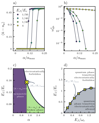
Figure 2: a) Order parameter $\big{<}\hat{n}-n_{g}\big{>}$ as a function of dissipation $\alpha$ (normalized to $\alpha_{\mathrm{max}}$) for four values of $E_{J}/E_{c}$, obtained at fixed $E_{J}/\omega_{c}=0.1$ and at the degeneracy point $n_{g}=1/2$. A quantum phase transition is only obtained if $E_{J}/E_{c}\ll 1$. b) Renormalized qubit frequency $\omega_{\mathrm{qb}}^{\star}$ for the same parameters, which vanishes at the same critical point. c) Phase diagram of the charge-boson model showing the phase boundary and the electrostatic forbidden regime ($E_{J}/\omega_{c}=0.1$ is fixed). d) General phase diagram for arbitrary $E_{J}/E_{c}$ and $E_{J}/\omega_{c}$, showing regimes where a spin-boson quantum phase transition for multilevel qubits is ruled out.

Computing the order parameter $\big{<}\hat{n}-n_{g}\big{>}$ can only be achieved by reliable quantum many-body simulations of the charge-boson Hamiltonian (2). Taking advantage of the impurity structure of the problem, we have extended the Numerical Renormalization Group (NRG) [56] to dissipative Josephson junctions, in contrast to previous treatments of the spin-boson model based on the two-level system approximation [57]. The method is based on an iterative diagonalization, adding modes one by one on a logarithmic grid, with a truncation of the Hilbert space at each NRG step. For the charge-boson model (2), the first stage of the NRG starts with the qubit degree of freedom, expressed in the charge basis, with up to $10^{3}$ charge states to ensure proper convergence for all considered $E_{J}/E_{c}$ values. We work with the Ohmic model $J(\omega)=2\pi\alpha\omega\exp{(-\omega/\omega_{c})}$ in units of $\omega_{c}=1$, and start the NRG procedure with frequencies of order $10\,\omega_{c}$ down to the minimal frequency $10^{-14}\omega_{c}$ that guarantees convergence of the NRG to the full many-body ground state.

Our first important finding concerns the dissipation-induced quantum phase transition of the charge-boson Hamiltonian (2), beyond the two-level approximation. Fig. 2a shows the ground state order parameter $\big{<}\hat{n}-n_{g}\big{>}$ as a function of normalized dissipation $\alpha/\alpha_{\mathrm{max}}$, which always stays zero when $E_{J}>E_{c}$. However, Cooper pair box qubits with $E_{c}\gg E_{J}$ do show a transition. This scenario is confirmed by monitoring the enhanced quantum fluctuations in the symmetric phase, from the charge response function $\chi(t)=\big{<}(\hat{n}(t)-n_{g})(\hat{n}(0)-n_{g})\big{>}$ of the qubit. A peak in the frequency domain occurs at the scale $\omega_{\mathrm{qb}}^{\star}$, associated to the renormalized frequency of the qubit. Extracting $\omega_{\mathrm{qb}}^{\star}$ for various parameter values, we see in Fig. 2b that $\omega_{\mathrm{qb}}^{\star}$ vanishes exponentially fast at the quantum critial point. Drawing the resulting phase diagram in the $(\alpha,E_{J}/E_{c})$ plane (here $E_{J}/\omega_{c}=0.1$ is fixed), we find in Fig. 2c that the transition point between the two phases simply disappears when $E_{J}/E_{c}$ is increased (cross), due to the border to the electrostatically forbidden region. Reporting the boundary $(E_{J}/E_{c})_{\mathrm{max}}$ in the $(E_{J}/E_{c},E_{J}/\omega_{c})$ plane, we obtain a completely general phase diagram in Fig. 2d. We thus established that the regime $E_{J}/E_{c}\gtrsim 1$ always forbids quantum criticality, so that the spin-boson paradigm does not apply for multilevel charge qubits, including transmons ($E_{J}\gg E_{c}$).

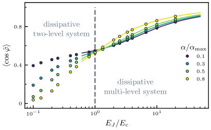
Figure 3: Josephson tunnelling $\big{<}\cos(\hat{\varphi})\big{>}$ in the ground state of the charge-boson model, comparing full NRG simulation (dots) with the simple Ansatz (7) (lines), computed as a function of $E_{J}/E_{c}$ for offset charge $n_{g}=1/2$ and several values of the normalized dissipation strength $\alpha/\alpha_{\mathrm{max}}$. Dissipation tends to localize the phase for multilevel charge qubits ($E_{J}>E_{c}$), namely $\big{<}\cos(\hat{\varphi})\big{>}$ increases with $\alpha$, while conversely phase delocalizes for two-level qubits ($E_{J}<E_{c}$). Surprisingly, zero point fluctuations are nearly dissipation insensitive in the crossover regime $E_{J}\simeq E_{c}$.

In the absence of a quantum phase transition, one may be tempted to conclude that the multilevel regime of dissipative qubits is trivial. On the contrary, it presents interesting many-body physics that we explore in the rest of this Letter. We investigate zero point fluctuations of the superconducting phase given by the average tunnelling $\big{<}\cos(\hat{\varphi})\big{>}$ in the many-body ground state. For transmons ($E_{J}\gg E_{c}$), $\big{<}\cos(\hat{\varphi})\big{>}$ increases with dissipation $\alpha$, because the phase is damped by its environment towards the minimum $\hat{\varphi}=0$ of the Josephson potential (this behavior is not captured by a two-level approximation [50]). In contrast, for a Cooper pair box ($E_{c}\gg E_{J}$) at the charge offset $n_{g}=1/2$, $\big{<}\cos(\hat{\varphi})\big{>}$ decreases with dissipation because charge fluctuations between $n=0$ and $n=1$ tend to freeze, so that, due to the Heisenberg principle, the phase delocalizes. This regime is strongly $n_{g}$ sensitive, since for $n_{g}=0$ the charge is already frozen in absence of dissipation. Both behaviors are clearly evidenced in Fig. 3, which shows $\big{<}\cos(\hat{\varphi})\big{>}$ against $E_{J}/E_{c}$, for several values of the normalized dissipation strength $\alpha/\alpha_{\mathrm{max}}$ at $n_{g}=0.5$ (dots are results from NRG simulations). Remarkably, the crossover is characterized by quantum fluctuations of the superconducting phase that are nearly dissipation-insensitive as seen by the narrowing spread of the points at $E_{J}=E_{c}$. This striking behavior is a manifestation of the frustrated nature of the qubit pointer states, that are neither purely phase-like nor purely charge-like in the crossover from multilevel to two-level qubits.

In order to capture physically these effects related to discrete charge, we finally develop a new description of dissipative multilevel qubits, since current polaronic theory [58, 59] applies mainly to the two-level regime. Obviously, dissipation tends to localize the phase in the multilevel regime, so that the wavefunction stays mosly trapped at the minima of the cosine Josephson potential. For $\varphi^{2}\ll 1$, the self-consistent harmonic approximation (SCHA) [60, 61, 13] replaces the cosine potential in (2) by an harmonic term:

$$\hat{H}_{\text{SCHA}}=\sum_{k}\omega_{k}\,\hat{a}^{\dagger}_{k}\hat{a}^{\phantom{\dagger}}_{k}+\hat{n}\sum_{k}ig_{k}(\hat{a}^{\dagger}_{k}-\hat{a}^{\phantom{\dagger}}_{k})+4E_{c}\hat{n}^{2}+\frac{E_{J}^{\star}}{2}\hat{\varphi}^{2},$$ (6)

which is nothing but the Caldera-Leggett model of a damped harmonic oscillator with renormalized Josephson energy $E_{J}^{\star}$. However, charge discreteness has to be taken into account via the compactness of the phase $\varphi\in[0,2\pi]$, which can be restored [62, 63] by periodizing the vacuum of $\hat{H}_{\text{SCHA}}$ (denoted $|0\rangle_{\text{SCHA}}$):

$$|0_{\circlearrowleft}\rangle=\sum_{w\in\mathbb{Z}}e^{i2\pi w\hat{n}}e^{-in_{g}\hat{\varphi}}|0\rangle_{\text{SCHA}},$$ (7)

including a gate offset $n_{g}$ associated to Aharonov-Casher interference [64]. After diagonalizing the linear Hamiltonian (6) in eigenmodes $b^{\dagger}_{\mu}$, $\hat{H}_{\text{SCHA}}=\sum_{\mu}\Omega_{\mu}\big{(}\hat{b}^{\dagger}_{\mu}\hat{b}^{\phantom{\dagger}}_{\mu}+\nicefrac{{1}}{{2}}\big{)}$, the qubit operators read $\hat{n}=i\sum_{\mu}v_{\mu}(b^{\dagger}_{\mu}-b_{\mu})$ and $\hat{\varphi}=\sum_{\mu}u_{\mu}(b^{\dagger}_{\mu}+b_{\mu})$ [50]. Using $E_{J}^{\star}$ as variational parameter, we estimate the ground state energy of Hamiltonian (2), and obtain analytically the tunneling:

$$\big{<}\!\cos(\hat{\varphi})\big{>}=\sum_{w\in\mathbb{Z}}\!\left[\frac{(\pi w)^{2}}{2}\!+\!(-1)^{w}e^{-\frac{u^{2}}{2}}\right]\!e^{-2(\pi w)^{2}v^{2}-i2\pi wn_{g}},$$ (8)

where $u^{2}\equiv\sum_{\mu}u_{\mu}^{2}$, $v^{2}\equiv\sum_{\mu}v_{\mu}^{2}$. The lines in Fig. 3 compare the full NRG simulations to the simple formula (8) in the range $E_{J}/E_{c}>1/2$, with excellent agreement. The crossover from multilevel to two-level regime results from a competition between two clear physical effects: 1) the Franck-Condon term $e^{-2\pi^{2}v^{2}w^{2}}$ associated to the winding number $w$ dual to the qubit charge $n$, weighting the overlaps between wells; 2) the Aharonov-Casher phase $e^{-i2\pi wn_{g}}$ associated to the gate charge $n_{g}$, driving interferences between wells.

In conclusion, we have demonstrated that realistic superconducting qubits do not show the same dissipative properties predicted from models based on the two-level approximation. We also provided a new physical picture of the many-body wavefunction for dissipative multilevel qubits, based on charge discreteness. Regarding experimental attempts at simulating quantum spins with superconducting circuits, we found that reaching the spin-boson quantum phase transition requires very strong non-linearities, well beyond the transmon regime. Similar considerations could apply to a wide class of model Hamiltonians that are touted as candidates for quantum simulators  [10, 13, 65, 41].

Supplementary Materials for “Spin-boson quantum phase transition in multilevel superconducting qubits”

I Microscopic parameters for the charge-boson model

In this section, we review one possible method for establishing the microscopic Hamiltonian from the circuit model, Eq. (4) of the main text. The starting point is the Lagrangian

$$\mathcal{L}=\frac{1}{2}\dot{\vec{\Phi}}^{\,{\vbox{\hbox{$\scriptstyle\intercal$}\nointerlineskip\hbox{}}}}\bm{C}\dot{\vec{\Phi}}-\frac{1}{2}\vec{\Phi}^{\,{\vbox{\hbox{$\scriptstyle\intercal$}\nointerlineskip\hbox{}}}}\nicefrac{{\bm{1}}}{{\bm{L}}}\,\vec{\Phi}+E_{J}\cos(\Phi_{0})-n_{g}\dot{\Phi}_{0},$$ (S1)

written in units of $\hbar=2e=1$, and with the capacitance and inductance matrices :

$$\,\bm{C}=\begin{bmatrix}C_{J}+C_{c}&-C_{c}&&&\\ -C_{c}&C+C_{c}+C_{g}&-C&&\\ &-C&2C+C_{g}&-C&\\ &&-C&\ddots&\ddots\\ &&&\ddots&\end{bmatrix},\quad{\nicefrac{{\bm{1}}}{{\bm{L}}}}=\frac{1}{L}\begin{bmatrix}0&0&&&\\ 0&1&-1&&\\ &-1&2&-1&\\ &&-1&\ddots&\ddots\\ &&&\ddots&\end{bmatrix}.$$ (S2)

We denoted here $C_{J}=C_{s}+C_{g}$ the combination of the shunting capacitance $C_{s}$ and ground capacitance $C_{g}$ of the qubit (see Fig. 1 of the main text).

Diagonalisation. A half-infinite chain is here assumed. We want to find a basis where both capacitance and inductance quadratic forms are diagonal. Since $\bm{C}$ is positive definite, this is equivalent to solving $\nicefrac{{\bm{1}}}{{\bm{L}}}\,\bm{P}=\bm{CP\omega}^{2}$ (a generalized eigenvalue problem). Under the change of basis $\vec{\Phi}=\bm{P}\vec{\phi}$, the Lagrangian is :

$$\mathcal{L}=\frac{1}{2}\dot{\vec{\phi}}^{\,{\vbox{\hbox{$\scriptstyle\intercal$}\nointerlineskip\hbox{}}}}\bm{P}^{\vbox{\hbox{$\scriptstyle\intercal$}\nointerlineskip\hbox{}}}\bm{CP}\dot{\vec{\phi}}-\frac{1}{2}\vec{\phi}^{\,{\vbox{\hbox{$\scriptstyle\intercal$}\nointerlineskip\hbox{}}}}\bm{P}^{\vbox{\hbox{$\scriptstyle\intercal$}\nointerlineskip\hbox{}}}\bm{CP\omega}^{2}\vec{\phi}+E_{J}\cos\left(\sum_{l}P_{0l}\phi_{l}\right)-n_{g}\sum_{l}P_{0l}\dot{\phi}_{l}.$$ (S3)

$\bm{P}^{\vbox{\hbox{$\scriptstyle\intercal$}\nointerlineskip\hbox{}}}\bm{CP}$ is diagonal, because it commutes with $\bm{\omega}^{2}$. We can then scale the eigenvectors to have $\bm{P}^{\vbox{\hbox{$\scriptstyle\intercal$}\nointerlineskip\hbox{}}}\bm{CP}=\openone$, and we reach Eq. (2) of the main text. Written explicitly, the generalized eigenvalue problem gives :

$$\text{site }i=0:\quad P_{1l}=\frac{C_{J}+C_{c}}{C_{c}}P_{0l},$$ (S4)

$$\text{site }i=1:\quad P_{2l}=P_{1l}\left(1-\frac{C_{f}}{C}\frac{\omega_{k_{l}}^{2}}{\omega_{0}^{2}-\omega_{k_{l}}^{2}}\right),\quad\text{with}\quad C_{f}=\frac{C_{c}C_{J}}{C_{c}+C_{J}}+C_{g}\quad\text{and}\quad\omega_{0}=\frac{1}{\sqrt{LC}},$$ (S5)

$$\text{site }i>1:\quad P_{i+1\,l}+P_{i-1\,l}=P_{il}\left(2-\frac{C_{g}}{C}\frac{\omega_{k_{l}}^{2}}{\omega_{0}^{2}-\omega_{k_{l}}^{2}}\right),$$ (S6)

where we parametrize the wavevector $k_{l}=\pi l/N_{\mathrm{modes}}$ of mode number $l$, with $N_{\mathrm{modes}}$ the number of modes (or sites in the chain). The eigenproblem is almost invariant by translation, except for the boundary condition. We assume that the solution obeys the form : $P_{jl}=N_{l}\cos{\left((j-1)k_{l}+\theta_{l}\right)}$, with $N_{l}$ the normalisation factor, and $\theta_{l}$ a phase shift due to the boundary. Note that $P_{0l}$ follows instead condition (S4), and therefore is not part of the parametrization, hence the ‘$(j-1)$’ labeling of the sites. In the half-infinite chain limit $N_{\mathrm{modes}}\to\infty$, the wavenumbers continuously fill the Brillouin zone : $k_{l}\in[0,\pi[$. The dispersion relation is obtained by injecting the solution in the bulk equation (S6), resulting in the standard expression:

$$\omega_{k_{l}}^{2}=\frac{4}{LC_{g}}\frac{\sin^{2}(k_{l}/2)}{1+4\left(C/C_{g}\right)\sin^{2}(k_{l}/2)}.$$ (S7)

Besides the dispersion relation, we also need $P_{0l}$, which appears in the coupling term between the charge qubit and the modes of the chain. The phase shift $\theta_{l}$ is imposed by the boundary equation (S5), used together with dispersion relation, and reads:

$$\tan\theta_{l}=\tan\left(\frac{k_{l}}{2}\right)\left(2\frac{C_{f}}{C_{g}}-1\right).$$ (S8)

Finally, we have to compute the normalization factors. First, one should note that the $k=0$ eigenfrequency is 0. Equations (S4), (S5), (S6) do not hold in this case, such that matrix elements $P_{i0}$ must be computed by normalization of $\bm{P}^{\vbox{\hbox{$\scriptstyle\intercal$}\nointerlineskip\hbox{}}}\bm{CP}$, which leads to $P_{00}=1/\sqrt{C_{J}+C_{c}},\quad P_{i0}=0\;\forall i>0$. This zero mode is then localized on the zeroth site: we recognize the qubit degree of freedom, which will be singled out as in the main text by a change of variable. The other normalisation factors are computed from the following matrix elements :

$$\forall l,l^{\prime}\neq 0,\quad\sum_{i,j=1}^{\infty}P_{il}C_{ij}P_{jl^{\prime}}=\left(C_{g}\sum_{i=1}^{\infty}P_{il}P_{il^{\prime}}+\frac{C_{c}C_{J}}{C_{c}+C_{J}}P_{1l}P_{1l^{\prime}}\right)\left(1+4\frac{C}{C_{g}}\sin^{2}(k_{l}/2)\right).$$ (S9)

This matrix must be diagonal, so we collect only the terms proportional to $\delta_{l,l^{\prime}}$. Expanding the first part as

$$\sum_{i=1}^{\infty}P_{il}P_{il^{\prime}}=\frac{1}{2}N_{l}N_{l^{\prime}}\sum_{j=0}^{\infty}\quad \cos(j(k_{l}+k_{l^{\prime}}))\cos(\theta_{l}+\theta_{l^{\prime}})+\cos(j(k_{l}-k_{l^{\prime}}))\cos(\theta_{l}-\theta_{l^{\prime}})$$

$$- \sin(j(k_{l}+k_{l^{\prime}}))\sin(\theta_{l}+\theta_{l^{\prime}})+\sin(j(k_{l}-k_{l^{\prime}}))\sin(\theta_{l}-\theta_{l^{\prime}}).$$ (S10)

Using the identity $\lim_{n\rightarrow\infty}\sum_{j=0}^{n}\cos(jk_{l})=\nicefrac{{1}}{{2}}+n\delta_{l,0}$ we can deduce the normalisation factor $N_{l}$. With equation (S4), we get an analytic expression of the couplings for a large but finite number of modes $N_{\mathrm{modes}}$:

$$P_{00}=\frac{1}{\sqrt{C_{J}+C_{c}}},\quad P_{0l}=\frac{C_{c}}{C_{J}+C_{c}}\sqrt{\frac{2}{N_{\mathrm{modes}}}}\left(C_{g}+4C\sin^{2}(k_{l}/2)\right)^{-\frac{1}{2}}\left(1+\left(2\frac{C_{f}}{C_{g}}-1\right)^{2}\tan^{2}(k_{l}/2)\right)^{-\frac{1}{2}}.$$ (S11)

These expressions match the results from the numerical diagonalization of the Lagrangian (S1) performed with a finite number $N_{\mathrm{modes}}$ of sites, as soon as $N_{\mathrm{modes}}\gtrsim 10$.

Hamiltonian form. Once in diagonal form, the Lagrangian (S3) reads

$$\mathcal{L}=\frac{1}{2}\sum_{k}\left(\dot{\phi}_{k}^{2}-\omega_{k}^{2}\phi_{k}^{2}\right)+E_{\rm J}\cos\left(\sum_{k}P_{0k}\phi_{k}\right)-n_{g}\sum_{k}P_{0k}\dot{\phi}_{k}.$$ (S12)

The Hamiltonian expression is obtained by Legendre transformation, using conjugate momenta $N_{k}=\partial\mathcal{L}/\partial\dot{\phi_{k}}$:

$$\mathcal{H}=\sum_{k}N_{k}\dot{\phi}_{k}-\mathcal{L}=\frac{1}{2}\sum_{k}\left((N_{k}+n_{g}P_{0k})^{2}+\omega_{k}^{2}\phi_{k}^{2}\right)-E_{\rm J}\cos\left(P_{0k}\phi_{k}\right).$$ (S13)

Canonical quantization is now straightforward : all dynamical variables are promoted to operators, obeying the commutation rule $[\phi_{k},N_{l}]=i\delta_{kl}$. In this Hamiltonian expression, the qubit degree of freedom does not appear explicitly. It can be reinstated following a change of variables that conserves the commutation rules:

$$\left\{\begin{array}[]{l}\varphi=\sum_{k}P_{0k}\phi_{k}\\ \varphi_{m}=\phi_{m}\end{array}\right.,\left\{\begin{array}[]{l}n=N_{0}/P_{00}\\ n_{m}=N_{m}-(P_{0m}/P_{00})N_{0}\end{array}\right.,$$ (S14)

where $\vec{n}$ (resp. $\vec{N}$) is the vector of charges conjugate to $\vec{\varphi}$ (resp. $\vec{\phi}$). As a result, we obtain the Hamiltonian:

$$\hat{H}=(P_{00}^{2}+\sum_{m}P_{0m}^{2})(\hat{n}-n_{g})^{2}+2(\hat{n}-n_{g})\sum_{m}P_{0m}\hat{n}_{m}+\frac{1}{2}\sum_{m}\left(\hat{n}_{m}^{2}+\omega_{m}^{2}\hat{\varphi}_{m}^{2}\right)-E_{\rm J}\cos(\hat{\varphi}).$$ (S15)

It is noteworthy that the change of variables does not complicate this expression, thanks to the fact that $\omega_{0}=0$ (this is a general feature of our model, because the qubit mode does not participate in the inductance matrix ${\bf L}$). Otherwise, $\omega_{0}^{2}\hat{\phi}_{0}^{2}$ would have transformed into:

$$\omega_{0}^{2}\hat{\phi}_{0}^{2}=\left(\frac{\omega_{0}}{P_{00}}\right)^{2}\hat{\varphi}^{2}+\left(\frac{\omega_{0}}{P_{00}}\right)^{2}\left(\sum_{m}P_{0m}\hat{\varphi}_{m}\right)^{2}-2\left(\frac{\omega_{0}}{P_{00}}\right)^{2}\hat{\varphi}\sum_{m}{\hat{\varphi_{m}}},$$ (S16)

the right-hand side terms being respectively interpreted as qubit inductive energy, a diamagnetic ‘$A^{2}$’ term, and a supplementary coupling between the qubit and the array. If present, these terms would violate phase compactness. Finally, the array normal modes are expressed in terms of creation/annihilation operators, defined by:

$$\hat{\varphi}_{m}=\frac{1}{\sqrt{2\omega_{m}}}(\hat{a}^{\dagger}_{m}+\hat{a}^{\phantom{\dagger}}_{m}),\quad\hat{n}_{m}=i\sqrt{\frac{\omega_{m}}{2}}(\hat{a}^{\dagger}_{m}-\hat{a}^{\phantom{\dagger}}_{m})\quad\text{and}\quad[\hat{a}^{\phantom{\dagger}}_{n},\hat{a}^{\dagger}_{m}]=\delta_{nm}.$$ (S17)

Spectral density. The bath spectral density gives a more convenient tool to describe this system with a small number of relevant parameters. It is defined as a continuous function of frequency, $J(\omega)=\pi\sum_{l}g_{k_{l}}^{2}\delta(\omega-\omega_{k_{l}})$. The $g_{k}$ couplings are defined in the main text as $g_{k_{l}}=\sqrt{\omega_{k_{l}}/2}P_{0l}$. All the dependencies in the wave number $k_{l}$ can be expressed in terms of $\omega_{k}$ using the dispersion relation (S7). We also change sums over modes to integrals in the limit $N_{\mathrm{modes}}\to\infty$:

$$\frac{1}{N_{\mathrm{modes}}}\sum_{l}F[k_{l}]\to\frac{1}{\pi}\int_{0}^{\pi}\!\!\!\mathrm{d}k\;F[k],$$ (S18)

$$J(\omega)=N_{\mathrm{modes}}\dfrac{\mathrm{d}{k}}{\mathrm{d}{\omega}}[g(\omega)]^{2}=\left(\frac{C_{c}}{C_{c}+C_{J}}\right)^{2}\sqrt{\frac{L}{C_{g}}}\ \omega\ \frac{\sqrt{1-\omega^{2}/\omega_{P}^{2}}}{1+\omega^{2}\left(1/\omega_{Q}^{2}-1/\omega_{P}^{2}\right)}\,\theta(\omega_{P}-\omega),$$ (S19)

with $\omega_{P}=\omega_{0}/\sqrt{1+4C/C_{g}}$ the plasma frequency of the chain, and $\omega_{Q}=\omega_{P}\sqrt{1+\nicefrac{{4C}}{{C_{g}}}}/(\nicefrac{{2C_{f}}}{{C_{g}}}-1)$ a characteristic frequency related to the qubit. From Eq. (S19), it is clear that the denominator is never vanishing within the band $\omega\in[0,\omega_{P}]$ (otherwise $J(\omega)$ would be singular). Using the expression for $\omega_{P}$ and $\omega_{Q}$, and $1/\omega_{J}^{2}\equiv 1/\omega_{Q}^{2}-1/\omega_{P}^{2}$, we recover the low frequency cutoff of the qubit $\omega_{J}$ defined in the main text.

For small frequencies, $J(\omega)$ obeys the so-called Ohmic behavior, $J(\omega)\simeq 2\pi\alpha\omega$, which defines the coupling strength $\alpha$. A higher frequencies, $J(\omega)$ quickly vanishes as $1/\omega^{2}$, provided $\omega_{J}\ll\omega_{P}$. Most experimental devices verify this condition. On the other hand, if $\omega_{J}\gg\omega_{P}$, $J(\omega)$ displays a square-root hard cut-off at $\omega=\omega_{P}$. In many cases, the exact form of the cut-off is not relevant, and we replace it by an exponential cut-off at $\omega_{c}=\min\left\{\omega_{J},\omega_{P}\right\}$, $J(\omega)=2\pi\alpha\omega\exp(-\omega/\omega_{c})$, which is the spectral function used in the main text to perform the numerical computations.

Microscopic derivation of the electrostatic bound on dissipation. The charging energy of our microscopic circuit explicitly reads

$$E_{c}=\frac{1}{8}\left(C_{J}+C_{c}-\frac{C_{c}^{2}}{C_{c}+\frac{C_{g}}{2}+\sqrt{C_{g}\left(\frac{C_{g}}{4}+C\right)}}\right)^{-1}.$$ (S20)

This result can be obtained by noting that $E_{c}=\bm{C}^{-1}_{00}/8$ and analytically inverting the capacitance matrix. From equation (5) in the main text one can reach the same result, recast into

$$8E_{c}=\frac{1}{C_{c}+C_{J}}+2\pi\alpha\frac{\omega_{J}^{2}}{\omega_{P}}\left(\sqrt{1+\frac{\omega_{P}^{2}}{\omega_{J}^{2}}}-1\right)\geqslant 2\pi\alpha\frac{\omega_{J}^{2}}{\omega_{P}}\left(\sqrt{1+\frac{\omega_{P}^{2}}{\omega_{J}^{2}}}-1\right),$$ (S21)

by integrating the spectral function (S19) over $\omega$. Thus the dissipation strength $\alpha$ obeys the inequality

$$\alpha\leqslant\frac{4E_{c}}{\pi\omega_{P}}\left(\sqrt{1+\frac{\omega_{P}^{2}}{\omega_{J}^{2}}}+1\right).$$ (S22)

When $\omega_{J}\ll\omega_{P}$ (which is the typical situation for realistic devices), the electrostatic bound $\alpha\leqslant 4E_{c}/(\pi\omega_{J})$ assumes the same form as in the main text (albeit with a different numerical prefactor), while for $\omega_{J}\gg\omega_{P}$ the bound reads $\alpha\leqslant 8E_{c}/(\pi\omega_{P})$.

II Compact ansatz wavefunction for charge sensitive circuits

We build in this section the compact ansatz step by step, following the outline of the main text. While our approach is completely generic to charge sensitive superconducting circuits, we focus here on the charge-boson Hamiltonian:

$$\hat{H}=4E_{c}(\hat{n}-n_{g})^{2}-E_{J}\cos\hat{\varphi}+(\hat{n}-n_{g})\sum_{k}ig_{k}(\hat{a}^{\dagger}_{k}-\hat{a}_{k})+\sum_{k}\omega_{k}\hat{a}^{\dagger}_{k}\hat{a}_{k},$$ (S23)

where the discrete sums over the wave vector $k$ run on the Brillouin zone $[0,\pi]$. The renormalized linear approximation, that holds only in the deep transmon regime where the phase fluctuations are much smaller that $2\pi$, is used as a linearized parent Hamiltonian for our variational trial state. It reads:

$$\hat{H}_{\mathrm{SCHA}}=4E_{c}\hat{n}^{2}+\frac{E_{J}^{\star}}{2}\hat{\varphi}^{2}+i\hat{n}\sum_{k}g_{k}(\hat{a}^{\dagger}_{k}-\hat{a}_{k})+\sum_{k}\omega_{k}\left(\hat{a}^{\dagger}_{k}\hat{a}_{k}+\nicefrac{{1}}{{2}}\right).$$ (S24)

Here the charge offset $n_{g}$ was gauged out since the phase is uncompact in the linear approximation, and $E_{J}^{\star}$ is a free parameter used in the variational method, after compactification is applied. This Hamiltonian can be brought to diagonal form by a Bogoliubov rotation mixing the qubit degree of freedom and bosons from the environment. For this purpose, we introduce rescaled charge $\hat{n}_{k}$ and phase $\hat{\phi}_{k}$ normal modes, so that $\hat{a}_{k}=(i\omega_{k}\hat{n}_{k}+\hat{\phi}_{k})/\sqrt{2\omega_{k}}$. We then lump these normal modes together with the qubit degree of freedom in the set charges $\hat{n}_{\mu}=(\hat{n},\hat{n}_{1},\hat{n}_{2},\ldots)$ and phases $\hat{\phi}_{\mu}=(\hat{\varphi},\hat{\phi}_{1},\hat{\phi}_{2},\ldots)$ (with greek indices), so that Hamiltonian (S24) reads:

$$\hat{H}_{\mathrm{SCHA}}=\frac{1}{2}\sum_{\mu}\hat{\phi}_{\mu}^{2}+\frac{1}{2}\sum_{\sigma\rho}\hat{n}_{\sigma}M_{\sigma\rho}\hat{n}_{\rho}\\ \qquad\text{where}\;\bm{M}=\begin{bmatrix}8E_{J}E_{c}&g_{1}\sqrt{2E_{J}\omega_{1}}&g_{2}\sqrt{2E_{J}\omega_{2}}&\ldots\\ g_{1}\sqrt{2E_{J}\omega_{1}}&\omega_{1}^{2}&&\\ g_{2}\sqrt{2E_{J}\omega_{2}}&&\omega_{2}^{2}&\\ \vdots&&&\ddots\end{bmatrix}.$$ (S25)

Diagonalization of the matrix $\bm{M}$, which assumes an arrowhead form, can be done efficiently from dedicated algorithms, as well as perturbative series expansion. We obtain $\bm{M}=\bm{O}\bm{D}\bm{O}^{\,{\vbox{\hbox{$\scriptstyle\intercal$}\nointerlineskip\hbox{}}}}$, with an orthonormal $\bm{O}$ matrix and a diagonal matrix $D_{\mu\nu}=\Omega_{\mu}^{2}\delta_{\mu\nu}$, introducing $\Omega_{\mu}$ the eigenfrequencies of the linear system. Defining new conjugate variables $\tilde{n}_{\mu}=\sum_{\nu}O_{\mu\nu}\hat{n}_{\nu}$ and $\tilde{\phi}_{\mu}=\sum_{\nu}O_{\mu\nu}\hat{\phi}_{\nu}$, we get:

$$\hat{H}_{\mathrm{SCHA}}=\frac{1}{2}\sum_{\mu}\left[\tilde{\phi}_{\mu}^{2}+\Omega_{\mu}^{2}\tilde{n}_{\mu}^{2}\right]=\sum_{\mu}\Omega_{\mu}\left[\hat{b}^{\dagger}_{\mu}\hat{b}^{\phantom{\dagger}}_{\mu}+\frac{1}{2}\right]$$ (S26)

where we introduced the destruction operators $\tilde{b}_{\mu}=(i\Omega_{\mu}\tilde{n}_{\mu}+\tilde{\phi}_{\mu})/\sqrt{2\Omega_{\mu}}$.

In order to perform the compactification of the qubit phase $\hat{\varphi}$, we express the qubit charge in terms of the final eigenmodes of $H_{\mathrm{SCHA}}$:

$$\hat{n} = \hat{n}_{0}=\sum_{\mu}O_{\mu 0}\tilde{n}_{\mu}=\sum_{\mu}O_{\mu 0}\sqrt{\frac{1}{2\Omega_{\mu}}}(\hat{b}^{\dagger}_{\mu}-\hat{b}^{\phantom{\dagger}}_{\mu})\equiv i\sum_{\mu}v_{\mu}(\hat{b}^{\dagger}_{\mu}-\hat{b}^{\phantom{\dagger}}_{\mu})$$ (S27)

$$\hat{\varphi} = \hat{\varphi}_{0}=\sum_{\mu}O_{\mu 0}\tilde{\varphi}_{\mu}=\sum_{\mu}O_{\mu 0}\sqrt{\frac{\Omega_{\mu}}{2}}(\hat{b}^{\dagger}_{\mu}+\hat{b}^{\phantom{\dagger}}_{\mu})\equiv\sum_{\mu}u_{\mu}(\hat{b}^{\dagger}_{\mu}+\hat{b}^{\phantom{\dagger}}_{\mu}).$$ (S28)

We then enforce the periodic boundary conditions (compactification) by repeatedly displacing the ground state of $H_{\rm SCHA}$, noted $|0\rangle$, by an integer times $2\pi$:

$$|0_{\circlearrowleft}\rangle=\sum_{w\in\mathbb{Z}}e^{i2\pi w\hat{n}}|0\rangle=\sum_{w\in\mathbb{Z}}e^{-2\pi w\sum_{\mu}v_{\mu}(\hat{b}^{\dagger}_{\mu}-\hat{b}^{\phantom{\dagger}}_{\mu})}|0\rangle,\quad\text{where }\hat{b}^{\phantom{\dagger}}_{\mu}|0\rangle=0\quad\forall\mu.$$ (S29)

Standard coherent state algebra in terms of the normal modes $\hat{b}^{\phantom{\dagger}}_{\mu}$ allows to readily compute expectations values from the compactified state (S29).

Regularisation. With such a definition, $|0_{\circlearrowleft}\rangle$ has infinite norm, because the associated wave function is both periodic and defined over $\mathbb{R}$. Indeed, by re-indexing sums over winding numbers,

$$\langle{0_{\circlearrowleft}}|{0_{\circlearrowleft}}\rangle=\sum_{v,w\in\mathbb{Z}}\int_{\mathbb{R}}\mathrm{d}\varphi\,\langle{0}|{\varphi-2\pi v}\rangle\langle{\varphi+2\pi w}|{0}\rangle=\langle{0}|{0_{\circlearrowleft}}\rangle\left(\sum_{v\in\mathbb{Z}}1\right),$$ (S30)

which is clearly infinite. A way out is to restrict the wave-function over the interval $[0,2\pi[$, which is in fact equivalent to simply drop the infinite factor in the last expression:

$$\langle{0}|{0_{\circlearrowleft}}\rangle\left(\sum_{v\in\mathbb{Z}}1\right)\xrightarrow[\text{to }[0,2\pi[]{\text{restricted}} \sum_{v,w\in\mathbb{Z}}\int_{0}^{2\pi}\mathrm{d}\varphi\,\langle{0}|{\varphi-2\pi v}\rangle\langle{\varphi+2\pi w}|{0}\rangle$$

$$=\sum_{v,w\in\mathbb{Z}}\int_{2\pi v}^{2\pi(v+1)}\mathrm{d}\varphi\,\langle{0}|{\varphi}\rangle\langle{\varphi+2\pi(v+w)}|{0}\rangle=\langle{0}|{0_{\circlearrowleft}}\rangle.$$ (S31)

The last line is obtained with a relabeling of the sums $w^{\prime}=w+v$, and patching the integrals together to get back an integral on $\mathbb{R}$. The same trick can be used for expectation values of any operator $\hat{\mathcal{O}}$, provided that it is itself $2\pi$-periodic, which means that $[\hat{\mathcal{O}},\sum_{w}\exp(i2\pi w\hat{n})]=0$.

Aharonov-Casher phases. We already mentioned that $n_{g}$ acts as a gauge potential on the system. It can usually be removed from the Hamiltonian by a gauge transformation $\hat{U}=\exp{(in_{g}\hat{\varphi})}$, which however affects the boundary condition on the phase (unless the model is not compact). Under such a transformation, $\hat{H}_{\mathrm{SCHA}}(n_{g})=\hat{U}^{\dagger}\hat{H}_{\mathrm{SCHA}}(0)\hat{U}$. It can be checked that $\hat{U}^{\dagger}|0\rangle$ is an eigenstate of $\hat{H}_{\mathrm{SCHA}}(n_{g})$. For a non-compact model, the gauge has no observable effect, but the compactification process will change this state of affairs, since

$$\sum_{w\in\mathbb{Z}}e^{i2\pi w\hat{n}}\hat{U}^{\dagger}|0\rangle=\hat{U}^{\dagger}\sum_{w\in\mathbb{Z}}e^{i2\pi w(\hat{n}-n_{g})}|0\rangle.$$ (S32)

As an example, the effect on the ansatz norm is :

$$\langle{0_{\circlearrowleft}}|{0_{\circlearrowleft}}\rangle=\sum_{v,w\in\mathbb{Z}}\langle 0|e^{-i2\pi v(\hat{n}-n_{g})}\hat{U}\hat{U}^{\dagger}e^{i2\pi w(\hat{n}-n_{g})}|0\rangle=\sum_{w\in\mathbb{Z}}e^{-i2\pi wn_{g}}\langle 0|e^{i2\pi w\hat{n}}|0\rangle,$$ (S33)

using $\hat{U}\hat{U}^{\dagger}=\openone$ and the same infinite factor canceling argument as before. The offset charge effect is seen as an Aharonov-Casher phase that depends on the winding number. The interference between different winding numbers will create an observable effect due to the gauge. The same argument can be used for the expectation value of any gauge invariant operator $\hat{\mathcal{O}}$, i.e. $[\hat{\mathcal{O}},\hat{U}]=0$.

$\mathbf{E_{\it J}^{\star}}$ optimisation. The anharmonicity of the $\cos$-shaped potential tends to soften the phase confinement compared to quadratic potential, thus enhancing the zero point phase fluctuations. Having built an ansatz adapted to the specifics of the problem, we can use it as starting point for a variational method. The free parameter is the effective stiffness of the potential $E_{J}^{\star}$ in the linearized Hamiltonian (S24). We need to compute the energy expectation value of the full Hamiltonian (S23) within the compactified ground state of the linearized Hamiltonian (S24). It is noteworthy that $\hat{H}$ is $2\pi$-periodic, but not gauge invariant. Instead, we make use of $\hat{U}\hat{H}(n_{g})\hat{U}^{\dagger}=\hat{H}(0)$. Using once again the decomposition (S28),

$$\frac{\langle 0_{\circlearrowleft}|\hat{H}|0_{\circlearrowleft}\rangle}{\langle{0_{\circlearrowleft}}|{0_{\circlearrowleft}}\rangle}=\sum_{\mu}\frac{\Omega_{\mu}}{2}-E_{J}\frac{u^{2}}{2}-E_{J}\left(\sum_{w\in\mathbb{Z}}e^{-2(\pi w)^{2}v^{2}-i2\pi wn_{g}}\right)^{-1}\sum_{w\in\mathbb{Z}}\left(\frac{(\pi w)^{2}}{2}+(-1)^{w}e^{-\frac{u^{2}}{2}}\right)e^{-2(\pi w)^{2}v^{2}-i2\pi wn_{g}}.$$ (S34)

The $E_{J}^{\star}$ dependence is contained in $u^{2}$ and $v^{2}$. The full numerical procedure consists, at every step, in a minimization of the expression (S34) over $E_{J}^{\star}$, using a fast diagonalization the arrowhead $\bm{M}$ matrix (S25) for the new value of $E_{J}^{\star}$, and the computation of the two scalars $u^{2}$ and $v^{2}$. We then compute the energy expectation value (S34) with a number of terms in the sums over $w$ controlled by $v^{2}$. Since the $w\neq 0$ terms are exponentially suppressed, the sums are rapidly convergent. In practice, we need at most $w\sim 10$ terms when the Josephson energy is close to the breaking point of the method, $E_{J}/E_{c}\sim 1$. Crucially, $u^{2}$ is independent of the number of modes. Overall, the complexity of the whole procedure is $\mathcal{O}(N_{\text{modes}}^{2})$, with $N_{\text{modes}}$ the total number of modes in the chain. The quality of the Ansatz is found to be excellent, see Fig. S1 for a comparison of the ground state energy obtained in the full NRG simulation.

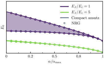
Figure S1: Ground state energy bands associated to the offset charge $n_{g}$, both for a multi-level charge qubit (narrower band at the bottom, at $E_{J}/E_{c}=5$) and the crossover regime (broaded band at the top, at $E_{J}/E_{c}=1$). The analytical expression (S34) from the compact Ansatz (lines) compares quantitatively to the full NRG simulation (dots).

Zero point phase fluctuations. Since $\cos\hat{\varphi}$ is both $2\pi$-periodic and gauge invariant, its expectation value is evaluated using the two previous tricks. Then, expressing every operator in terms of $\hat{b}^{\dagger}_{\mu},\hat{b}^{\phantom{\dagger}}_{\mu}$ with (S28) :

$$\langle 0_{\circlearrowleft}|\cos\hat{\varphi}|0_{\circlearrowleft}\rangle =\frac{1}{2}\sum_{\pm,w\in\mathbb{Z}}e^{-i2\pi wn_{g}}\langle 0|\exp\Big{(}\pm i\sum_{\sigma}u_{\sigma}(\hat{b}^{\dagger}_{\sigma}+\hat{b}^{\phantom{\dagger}}_{\sigma})\Big{)}\exp\Big{(}-2\pi w\sum_{\rho}v_{\rho}(\hat{b}^{\dagger}_{\rho}-\hat{b}^{\phantom{\dagger}}_{\rho})\Big{)}|0\rangle$$

$$=e^{-\frac{1}{2}\sum_{\nu}(u_{\nu})^{2}}\sum_{w}(-1)^{w}e^{-2(\pi w)^{2}\sum_{\mu}(v_{\mu})^{2}-i2\pi wn_{g}}.$$ (S35)

Note that since the state norm isn’t unity, normalization is necessary, by a factor $\langle{0_{\circlearrowleft}}|{0_{\circlearrowleft}}\rangle=\sum_{w}\exp(-2(\pi w)^{2}v^{\mu}v_{\mu})$. Clearly, $v^{2}\equiv\sum_{\mu}(v^{\mu})^{2}$ weights the corrections from non-zero winding numbers. It vanishes when $E_{J}\rightarrow\infty$, providing a pure harmonic oscillator behavior in this limit. At finite $E_{J}$, it sets the number of windings taken into account to reach required numerical accuracy. In the same fashion, $u^{2}\equiv\sum_{\mu}(u^{\nu})^{2}$ renormalizes the bare Josephson energy, $E_{J}^{\prime}=E_{J}\exp(-u^{2}/2)$ (note that the previously defined term $E_{J}^{\star}$ appears only in the linearized Hamiltonian used to derive the ansatz, and acts only as a variational parameter).

III Perturbation theory at small coupling strength.

One of the charge-boson model’s striking features is the different responses of the junction’s phase fluctuations $\langle\cos\hat{\varphi}\rangle$ to coupling strength $\alpha$, depending of the $E_{J}/E_{c}$ regime, as shown by Fig. 3 of the main text. Broadly speaking, the environment damps the phase fluctuations of the dissipative multi-level charge qubits, but enhances those of the dissipative two-level system. As already emphasized, this behavior cast doubt on the two-level description of dissipative multi-level qubits. Arguably, while this feature is correctly described by both NRG and our compact ansatz, a simple perturbative analysis in $\alpha$ should already be able to discriminate between these two regimes, and pin-point the break down of the two-level approximation.

We employ time-independent perturbation theory at second order, with $(\hat{n}-\nicefrac{{1}}{{2}})\sum_{k}ig_{k}(\hat{a}^{\dagger}_{k}-\hat{a}^{\phantom{{\dagger}}}_{k})$ as the perturbation. We denote $|\psi_{n}\rangle$ the eigenstates of the bare qubit, $E_{n}$ their energies. Then,

$$\left\langle\cos\hat{\varphi}\right\rangle\simeq\langle 0|\cos\hat{\varphi}|0\rangle +\sum_{\begin{subarray}{c}k\\ n\neq 0\\ m\neq 0\end{subarray}}g_{k}^{2}\frac{\langle\psi_{n}|\hat{n}|\psi_{0}\rangle\langle\psi_{0}|\hat{n}|\psi_{m}\rangle}{(E_{0}-E_{n}-\omega_{k})(E_{0}-E_{m}-\omega_{k})}\langle\psi_{n}|\cos\hat{\varphi}|\psi_{m}\rangle-\sum_{\begin{subarray}{c}k\\ n\neq 0\end{subarray}}g_{k}^{2}\frac{|\langle\psi_{n}|\hat{n}|\psi_{0}\rangle|^{2}}{(E_{0}-E_{n}-\omega_{k})^{2}}\langle\psi_{0}|\cos\hat{\varphi}|\psi_{0}\rangle$$

$$+2\sum_{\begin{subarray}{c}k,j,\\ i\neq 0\end{subarray}}g_{k}^{2}\frac{\langle\psi_{0}|\cos\hat{\varphi}|\psi_{i}\rangle\langle\psi_{j}|\hat{n}|\psi_{0}\rangle\langle\psi_{j}|\hat{n}|\psi_{i}\rangle}{(E_{0}-E_{i})(E_{0}-E_{J}-\omega_{k})}.$$ (S36)

This expression takes into account the multi-level nature of the qubit. It can be reduced by restricting the sum on bare qubit levels to the most significant element:

$$\left\langle\cos\hat{\varphi}\right\rangle\simeq\langle 0|\cos\hat{\varphi}|0\rangle +\sum_{k}g_{k}^{2}\frac{|\langle\psi_{1}|\hat{n}|\psi_{0}\rangle|^{2}}{(E_{0}-E_{1}-\omega_{k})^{2}}\langle\psi_{1}|\cos\hat{\varphi}|\psi_{1}\rangle-\sum_{k}g_{k}^{2}\frac{|\langle\psi_{1}|\hat{n}|\psi_{0}\rangle|^{2}}{(E_{0}-E_{1}-\omega_{k})^{2}}\langle\psi_{0}|\cos\hat{\varphi}|\psi_{0}\rangle$$

$$+2\sum_{k}g_{k}^{2}\frac{\langle\psi_{1}|\hat{n}|\psi_{0}\rangle\langle\psi_{1}|\hat{n}|\psi_{2}\rangle}{(E_{0}-E_{2})(E_{0}-E_{1}-\omega_{k})}\langle\psi_{2}|\cos\hat{\varphi}|\psi_{0}\rangle.$$ (S37)

The first and second term correspond to the two-level approximation (in the limit $\alpha\to 0$). However, the third term adds the contribution from the third qubit level into the mix. Indeed, this term is mostly responsible for the qualitative change between dissipative two- and multi-level qubits when $E_{J}/E_{c}$ is increased, as shown by the Fig. S2.

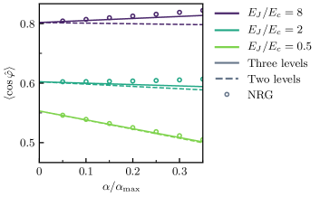
Figure S2: NRG estimates for phase fluctuations as a function of $\alpha$ (circles), compared to the two and three levels approximation within first order perturbation theory (dashed and solid lines respectively). The two levels approximation (dashed lines) clearly fails for tmulti-level qubits, where the slope changes of sign, while bringing the third level improves the agreement to NRG.