Variance-Reduced Methods for Machine Learning

Abstract

Stochastic optimization lies at the heart of machine learning, and its cornerstone is stochastic gradient descent (SGD), a method introduced over 60 years ago. The last 8 years have seen an exciting new development: variance reduction (VR) for stochastic optimization methods. These VR methods excel in settings where more than one pass through the training data is allowed, achieving a faster convergence than SGD in theory as well as practice. These speedups underline the surge of interest in VR methods and the fast-growing body of work on this topic. This review covers the key principles and main developments behind VR methods for optimization with finite data sets and is aimed at non-expert readers.

ssss

1 Introduction

One of the fundamental problems studied in the field of machine learning is how to fit models to large datasets. For example, consider the classic linear least squares model,

$$x_{\star}\in\operatorname*{\arg\!\min}_{x\in\mathbb{R}^{d}}\left\{\frac{1}{n}\sum_{i=1}^{n}(a_{i}^{\top}x-b_{i})^{2}\right\}.$$ (1)

Here, the model has $d$ parameters given by the vector $x\in\mathbb{R}^{d}$ and we are given $n$ data points $\{a_{i},b_{i}\}$ consisting of feature vectors $a_{i}\in\mathbb{R}^{d}$ and target values (labels) $b_{i}\in\mathbb{R}$. Fitting the model consists of tuning these $d$ parameters so that the model’s output $a_{i}^{\top}x$ is “close” (on average) to the targets $b_{i}$. More generally, we might use some loss function $f_{i}(x)$ to measure how close our model is to the $i$-th data point,

$$x_{\star}\in\operatorname*{\arg\!\min}_{x\in\mathbb{R}^{d}}\left\{f(x):=\frac{1}{n}\sum_{i=1}^{n}f_{i}(x)\right\}.$$ (2)

If $f_{i}(x)$ is large, we say that our model’s output is far from the data, and if $f_{i}(x)=0$ we say that our model fits perfectly the $i$-th data point. The function $f(x)$ represents the average loss of our model over the full dataset. A problem of the form (2) characterizes the training of not only linear least squares, but many models studied in machine learning. For example, the logistic regression model solves

$$x_{\star}\in\operatorname*{\arg\!\min}_{x\in\mathbb{R}^{d}}\left\{\frac{1}{n}\sum_{i=1}^{n}\log(1+\exp(-b_{i}a_{i}^{\top}x))+\frac{\lambda}{2}{\left\|x\right\|}^{2}\right\},$$ (3)

where we are now considering a binary classification task with $b_{i}\in\{-1,+1\}$ (and predictions are made using the sign of $a_{i}^{\top}x$). Here, we have also used $\frac{\lambda}{2}{\left\|x\right\|}^{2}:=\frac{\lambda}{2}\sum_{i=1}^{d}x_{i}^{2}$, as a regularizer. This and other regularizers are commonly added to avoid overfitting to the given data, and in this case we replace each $f_{i}(x)$ by $f_{i}(x)+\frac{\lambda}{2}{\left\|x\right\|}^{2}$. The training procedure in most supervised machine learning models can be written in the form (2), including L1-regularized least squares, support vector machines, principal component analysis, conditional random fields, and deep neural networks.

A key challenge in modern instances of problem (2) is that the number of data points $n$ can be extremely large. We regularly collect datasets going beyond terabytes, from sources such as the internet, satellites, remote sensors, financial markets, and scientific experiments. One of the most common ways to cope with such large datasets is to use stochastic gradient descent (SGD) methods, which use a few randomly chosen data points in each of their iterations. Further, there has been a recent surge in interest in variance-reduced (VR) stochastic gradient methods which converge faster than classic stochastic gradient methods.

1.1 Gradient and Stochastic Gradient Descent

The classic GD (gradient descent) method applied to problem (2) takes the form

$$x_{k+1}=x_{k}-\gamma\frac{1}{n}\sum_{i=1}^{n}\nabla f_{i}(x_{k}),$$ (4)

where $\gamma>0$ is a fixed stepsize. At each iteration the GD method needs to calculate a gradient $\nabla f_{i}(x_{k})$ for every $i$th data point, and thus GD takes a full pass over the $n$ data points at each iteration. This expensive cost per iteration makes GD prohibitive when $n$ is large.

Consider instead the stochastic gradient descent (SGD) method,

$$x_{k+1}=x_{k}-\gamma\nabla f_{i_{k}}(x_{k}),$$ (5)

first introduced by Robbins and Monro, (1951). It avoids the heavy cost per iteration of GD by using one randomly-selected $\nabla f_{i_{k}}(x_{k})$ gradient instead of the full gradient. In Figure 1, we see how the SGD method makes dramatically more progress than GD (and even the “accelerated” GD method) in the initial phase of optimization.

1.2 The Issue with Variance

Observe that if we choose the random index $i_{k}\in\{1,\ldots,n\}$ uniformly, $\mathbf{P}\left[i_{k}=i\right]=\frac{1}{n}$ for all $i$, then $\nabla f_{i_{k}}(x_{k})$ is an unbiased estimate of $\nabla f(x_{k})$ since

$${\mathbf{E}\left[\nabla f_{i_{k}}(x_{k})\;|\;x_{k}\right]} =\sum_{i=1}^{n}\frac{1}{n}\nabla f_{i}(x_{k})=\nabla f(x_{k}).$$ (6)

Thus, even though the SGD method is not guaranteed to decrease $f$ in each iteration, on average the method is moving in the direction of the negative full gradient, which is a direction of descent.

Unfortunately, having an unbiased estimator of the gradient is not enough to guarantee convergence of the iterates (5) of SGD. To illustrate this, in Figure 2 (left) we have plotted the iterates of SGD with a constant stepsize applied to a logistic regression function using the fourclass data set from LIBSVM (Chang and Lin,, 2011). The concentric ellipses in Figure 2 are the level sets of this function, that is, the points $x$ on a single ellipse are given by $\{x\,:\,f(x)=c\}$ for a particular constant $c\in\mathbb{R}.$ Different constants $c$ give different ellipses.

The iterates of SGD do not converge to the solution (the green star), and instead form a point cloud around the solution. In contrast, we have plotted the iterates of a VR method SAG (that we present later) in Figure 2 using the same constant stepsize.

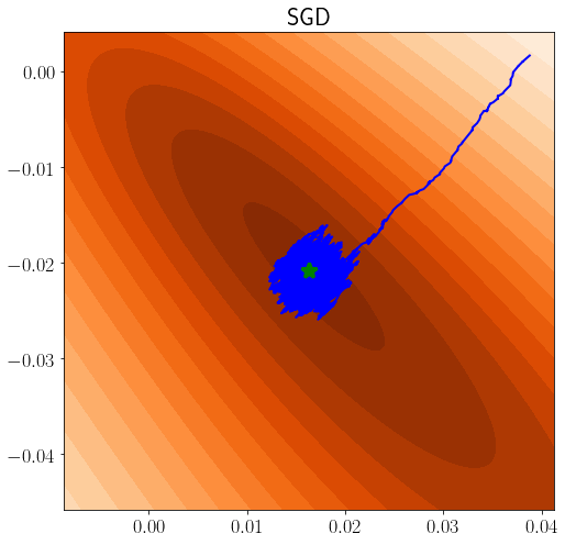
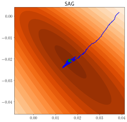
Figure 2: Level set plot of 2D logistic regression with the iterates of SGD (left) and SAG (right) with constant stepsize. The green star is the $x_{*}$ solution.

The reason why SGD does not converge in this example is because the stochastic gradients themselves do no converge to zero, and thus the method (5) with a constant stepsize never stops. This is in contrast with GD, where the method naturally stops since $\nabla f(x_{k})\rightarrow 0$ as $x_{k}\rightarrow x_{\star}$.

1.3 Classic Variance Reduction Methods

There are several classic techniques for dealing with the non-convergence due to the variance in the $\nabla f_{i}(x_{k})$ values. For example, Robbins and Monro, (1951) address the issue of the variance using a sequence of decreasing stepsizes $\gamma_{k}$. This forces the product $\gamma_{k}\nabla f_{i_{k}}(x_{k})$ to converge to zero. However it is difficult to tune this sequence of decreasing stepsizes so that the method does not stop to early (before reaching the solution) or to late (thus wasting resources).

Another classic technique for decreasing the variance is to use the average of several $\nabla f_{i}(x_{k})$ values in each iteration to get a better estimate of the full gradient $\nabla f(x)$. This is called mini-batching, and is especially useful when multiple gradients can be evaluated in parallel. This leads to an iteration of the form

$$x_{k+1}=x_{k}-\gamma\frac{1}{|B_{k}|}\sum_{i\in B_{k}}\nabla f_{i}(x_{k}),$$ (7)

where $B_{k}\subset\{1,\ldots,n\}$ is a set of random indices and $|B_{k}|$ is the size of $B_{k}$. the variance of this gradient estimator is inversely proportional to the “batch size” $|B_{k}|$, so we can decrease the variance by increasing the batch size. However, the cost of this iteration is proportional to the batch size. Thus, this form of variance reduction comes at a computational cost.

Yet another common strategy to decrease variance and improve the empirical performance of SGD is to add “momentum”, an extra term based on the directions used in past steps. In particular, SGD with momentum takes the form

$$m_{k} =\beta m_{k-1}+\nabla f_{i_{k}}(x_{k})$$ (8)

$$x_{k+1} =x_{k}-\gamma m_{k},$$ (9)

where the momentum parameter $\beta$ is in the range $(0,1)$. Setting $m_{0}=0$ and expanding the update of $m_{k}$ in (8) we have that $m_{k}$ is a weighted average of the previous gradients,

$$m_{k}=\sum_{t=0}^{k}\beta^{k-t}\nabla f_{i_{t}}(x_{t}).$$ (10)

Thus $m_{k}$ is a weighted sum of the stochastic gradients. Moreover since $\sum_{t=0}^{k}\beta^{k-t}=\frac{1-\beta^{k+1}}{1-\beta}$, we have that $\frac{1-\beta}{1-\beta^{k-1}}m_{k}$ is a weighted average of stochastic gradients. If we compare this with the expression of the full gradient which is a plain average, $\nabla f(x_{k})=\frac{1}{n}\sum_{i=1}^{n}\nabla f_{i}(x_{k})$, we can interpret $\frac{1-\beta}{1-\beta^{k}}m_{k}$ (and $m_{k})$ as an estimate of the full gradient. This weighted sum decreases the variance but it also brings about a key problem: Since the weighted sum (10) gives more weight to recently sampled gradients, it does not converge to the full gradient $\nabla f(x_{k})$ which is a plain average. The first variance reduced method we will see in Section 2.2.1 contours this issue by using a plain average, as opposed to any weighted average.

1.4 Modern Variance Reduction Methods

As opposed to classic methods that use one or more $\nabla f_{i}(x_{k})$ directly as an approximation of $\nabla f(x_{k}),$ variance-reduced methods use $\nabla f_{i}(x_{k})$ to update an estimate $g_{k}\in\mathbb{R}^{d}$ of the gradient so that $g_{k}\approx\nabla f(x_{k})$. With this gradient estimate, we then take approximate gradient steps of the form

$$x_{k+1}=x_{k}-\gamma g_{k},$$ (11)

where $\gamma>0$ is again the stepsize. To make (11) converge with a constant stepsize, we need to ensure that the variance of our gradient estimate $g_{k}$ converges to zero, that is

$${\mathbf{E}\left[{\left\|g_{k}-\nabla f(x_{k})\right\|}^{2}\right]}\quad\underset{k\rightarrow\infty}{\longrightarrow}\quad 0,$$ (12)

where the expectation is taken with respect to all the random variables in the algorithm up to iteration $k.$ Property (12) ensures that the VR method will stop when reaching the optimal point. We take (12) to be a defining property of variance-reduced methods and thus refer to it as the VR property. Note that “reduced” variance is a bit misleading since the variance converges to zero. The property (12) is responsible for the faster convergence of VR methods in theory (under suitable assumptions) and in practice as we see in Figure 1.

1.5 First example of a VR method: SGD_⋆

One easy fix that makes the SGD recursion in (5) converge without decreasing the stepsize is to simply shift each gradient by $\nabla f_{i}(x_{\star})$, that is, to use the following method

$$x_{k+1}=x_{k}-\gamma\left(\nabla f_{i_{k}}(x_{k})-\nabla f_{i_{k}}(x_{\star})\right),$$ (13)

called SGD_⋆ (Gorbunov20unified). We note that it is unrealistic that we would know each $\nabla f_{i}(x_{\star})$, but we use SGD_⋆ as a simple illustration of the properties of VR methods. Further, many VR methods can be seen as an approximation of the SGD_⋆ method; instead of relying on knowing each $\nabla f_{i}(x_{\star})$, these methods use approximations that converge to $\nabla f_{i}(x_{\star})$.

Note that SGD_⋆ uses an unbiased estimate of the full gradient. Indeed, since $\nabla f(x_{\star})=0$,

$${\mathbf{E}\left[\nabla f_{i_{k}}(x_{k})-\nabla f_{i_{k}}(x_{\star})\right]}=\nabla f(x_{k})-\nabla f(x_{\star})=\nabla f(x_{k}).$$

Furthermore, SGD_⋆ naturally stops when it reaches the optimal point since, for any $i$,

$$\left.\big{(}\nabla f_{i}(x)-\nabla f_{i}(x_{\star})\big{)}\right|_{x=x_{\star}}=0.$$

Next, we note that SGD_⋆ satisfies the VR property (12) as $x_{k}$ approaches $x_{\star}$ (for continuous $\nabla f_{i}$) since

$${\mathbf{E}\left[{\left\|g_{k}-\nabla f(x_{k})\right\|}^{2}\right]} ={\mathbf{E}\left[{\left\|\nabla f_{i}(x_{k})-\nabla f_{i}(x_{\star})-\nabla f(x_{k})\right\|}^{2}\right]}$$

$$\leq{\mathbf{E}\left[{\left\|\nabla f_{i}(x_{k})-\nabla f_{i}(x_{\star})\right\|}^{2}\right]},$$

where we used Lemma A.2 with $X=\nabla f_{i}(x_{k})-\nabla f_{i}(x_{\star})$ and then used that ${\mathbf{E}\left[\nabla f_{i}(x_{k})-\nabla f_{i}(x_{\star})\right]}=\nabla f(x_{k})$. This property implies that SGD_⋆ has a faster convergence rate than classic SGD methods, as we detail in Appendix B.

1.6 Faster Convergence of VR Methods

In this section we introduce two standard assumptions that are used to analyze VR methods, and discuss the speedup over classic SGD methods that can be obtained under these assumptions. Our first assumption is Lipschitz continuity of the gradients, meaning that the gradients cannot change arbitrarily fast.

While this is typically viewed as a weak assumption, in Section 4 we comment on VR methods that apply to non-smooth problems. This $L$-smoothness assumption has an intuitive interpretation for univariate functions that are twice-differentiable: it is equivalent to assuming that the second derivative is bounded by $L$, $|f^{\prime\prime}(x)|\leq L$ for every $x\in\mathbb{R}^{d}$. For multivariate twice-differentiable functions, it is equivalent to assuming that the singular values of the Hessian matrix $\nabla^{2}f(x)$ are upper bounded by $L$ for every $x\in\mathbb{R}^{d}$. For the least squares problem (1), the individual Lipschitz constants $L_{i}$ are given by $L_{i}={\left\|a_{i}\right\|}^{2}$, while for the L2-regularized logistic regression problem (3), we have $L_{i}=0.25{\left\|a_{i}\right\|}^{2}+\lambda$.

The second assumption we consider in this section lower bounds the curvature of the functions.

This is a strong assumption. While each $f_{i}$ is convex in the least squares problem (1), the overall function $f$ is strongly convex if and only if the design matrix $A:=[a_{1},\ldots,a_{n}]$ has full row rank. On other hand, the L2-regularized logistic regression problem (3) satisfies this assumption with $\mu\geq\lambda$ due to the presence of the regularizer. As we detail in Section 4, it is possible to relax the strong convexity assumption as well as the assumption that each $f_{i}$ is convex.

An important problem class where the assumptions are satisfied are problems of the form

$$x_{\star}\in\operatorname*{\arg\!\min}_{x\in\mathbb{R}^{d}}\left\{f(x)=\frac{1}{n}\sum_{i=1}^{n}\ell_{i}(a_{i}^{\top}x)+\frac{\lambda}{2}{\left\|x\right\|}^{2}\right\}$$ (15)

in the case when each “loss” function $\ell_{i}:\mathbb{R}\mapsto\mathbb{R}$ is twice-differentiable with $\ell_{i}^{\prime\prime}$ bounded between $0$ and some upper bound $M$. This includes a variety of loss functions with L2-regularization in machine learning, such as least squares ($l_{i}(\alpha)=(\alpha-b_{i})^{2}$), logistic regression, probit regression, Huber robust regression, and a variety of others. In this setting, for all $i$ we have $L_{i}\leq M{\left\|a_{i}\right\|}^{2}+\lambda$ and $\mu\geq\lambda$.

The convergence rate of GD under these assumptions is determined by the ratio $\kappa:=L/\mu$, which is known as the condition number of $f$. This ratio is always greater or equal to one, and when it is significantly larger than one, the level sets of the function become very elliptical which causes the iterates of the GD method to oscillate. This is illustrated in Figure 3. In contrast, when $\kappa$ is close to 1, GD converges quickly.

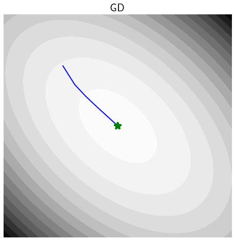
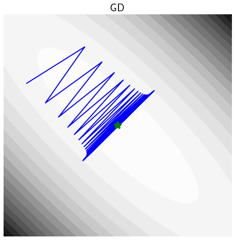
Figure 3: Here we graph the level sets two logistic regression loss functions. The left level sets are each of a well-conditioned logistic function with $\kappa\approx 1.$ The right level sets are of an ill-conditioned logistic functions with $\kappa\gg 1.$

Under Assumptions 1.1 and 1.2, VR methods converge at a linear rate. We say that the function values $\{f(x_{k})\}$ of a randomized method converge linearly (in expectation) at a rate of $0<\rho\leq 1$ if there exists a constant $C>0$ such that

$${\mathbf{E}\left[f(x_{k})\right]}-f(x_{\star})\leq(1-\rho)^{k}C={\cal O}(\exp(-k\rho)),\quad\forall k.$$ (16)

This is in contrast to classic SGD methods that only rely on an unbiased estimate of the gradient in each iteration, which under these assumptions can only obtain the sublinear rate

$${\mathbf{E}\left[f(x_{k})\right]}-f(x_{\star})\leq{\cal O}(1/k).$$

Thus, classic SGD methods become slower the longer we run them, while VR methods continue to cut the error by at least a fixed fraction in each step.

As a consequence of (16), we can determine the number of iterations needed to reach a given tolerance $\varepsilon>0$ on the error as follows

$$k\;\geq\;\frac{1}{\rho}\log\left(\frac{C}{\varepsilon}\right),\quad\mbox{then}\quad{\mathbf{E}\left[f(x_{k})\right]}-f(x_{\star})\leq\varepsilon.$$ (17)

The smallest $k$ satisfying this inequality is known as the iteration complexity of the algorithm. Below we give the iteration complexity and the cost of one iteration in terms of $n$ for the basic variant of GD, SGD, and VR methods:

Algorithm	# Iterations	Cost of 1 Iteration
GD	${\cal O}(\kappa\log(1/\varepsilon))$	${\cal O}(n)$
SGD	${\cal O}((1/\varepsilon))$	${\cal O}(1)$
VR	${\cal O}((\kappa_{\max}+n)\log(1/\varepsilon))$	${\cal O}(1)$

The total runtime of an algorithm is given by the product of the iteration complexity and the iteration runtime. Above we have used $\kappa_{\max}:=(\max_{i}L_{i})/\mu$. Note that $\kappa_{\max}\geq\kappa$, thus the iteration complexity of GD is smaller than that of the VR methods. But the VR methods are superior in terms of total runtime since each iteration of gradient descent costs $n$-times more than an iteration of a VR method. Classic SGD methods have the advantage that their runtime and their convergence rate does not depend on $n$, but it does have a much worse dependency on the tolerance $\varepsilon$ which explains SGD’s poor performance when the tolerance is small.

In Appendix B we give a simple proof showing that the SGD_⋆ method has the same iteration complexity as the VR methods.

2 Basic Variance-Reduced Methods

The first wave of variance-reduced methods that achieve the convergence rate from the previous section started with the stochastic average gradient (SAG) method (Le Roux et al.,, 2012; Schmidt et al.,, 2017). This was followed shortly after by the stochastic dual coordinate ascent (SDCA) (Richtárik and Takáč,, 2014; Shalev-Shwartz and Zhang,, 2013), MISO (Mairal,, 2015), stochastic variance-reduced gradient (SVRG/S2GD) (Mahdavi and Jin,, 2013; Johnson and Zhang,, 2013; Konecný and Richtárik,, 2013; Zhang et al.,, 2013), and SAGA  (Defazio et al.,, 2014) methods. In this section we present several of these original methods, while Section 4 covers more recent methods that offer improved properties in certain settings over these original methods.

2.1 Stochastic Average Gradient (SAG)

The first VR method is based on mimicking the structure of the full gradient. Since the full gradient $\nabla f(x)$ is a plain average of the $\nabla f_{i}(x)$ gradients, our estimate $g_{k}$ of the full gradient should be an average of estimates of the $\nabla f_{i}(x)$ gradients. This idea leads us to our first variance-reduced method: the stochastic average gradient (SAG) method.

The stochastic average gradient (SAG) method (Le Roux et al.,, 2012; Schmidt et al.,, 2017) is a stochastic variant of the earlier incremental aggregated gradient (IAG) method (Blatt et al.,, 2007). The idea behind SAG is to maintain an estimate $v_{k}^{i}\approx\nabla f_{i}(x_{k})$ for each data point $i$. We then use the average of the $v_{k}^{i}$ values as our estimate of the full gradient, that is

$$\bar{g}_{k}=\frac{1}{n}\sum_{j=1}^{n}v_{k}^{j}\approx\frac{1}{n}\sum_{j=1}^{n}\nabla f_{j}(x_{k})=\nabla f(x_{k}).$$ (18)

At each iteration, SAG samples $i_{k}\in\{1,\ldots,n\}$ and updates the $v_{k}^{j}$ using

$$v_{k+1}^{j}=\begin{cases}\nabla f_{i_{k}}(x_{k})&\quad\mbox{if }j=i_{k}\,,\\ v_{k}^{j}&\quad\mbox{if }j\neq i_{k}\,,\end{cases}$$ (19)

where each $v^{0}_{i}$ might be initialized to zero or to an approximation of $\nabla f_{i}(x_{0})$. As we approach a solution $x_{\star}$, each $v^{i}$ converges to $\nabla f_{i}(x_{\star})$ which gives us the VR property (12).

To implement SAG efficiently, we need to take care in computing $\bar{g}_{k}$ using (18), since this requires summing up $n$ vectors in $\mathbb{R}^{d}$, and since $n$ can be very large, computing this sum can be very costly. Fortunately we can avoid computing this summation from scratch every iteration since only one $v_{k}^{i}$ term will change in the next iteration. That is, suppose we sample the index $i_{k}$ on iteration $k$. It follows from (18) and (19) that

$$\bar{g}_{k} =\frac{1}{n}\sum_{j=1,j\neq i_{k}}^{n}v_{k}^{j}+\frac{1}{n}v_{k}^{i_{k}}$$

$$=\frac{1}{n}\sum_{j=1,j\neq i_{k}}^{n}v_{k-1}^{j}+\frac{1}{n}v_{k}^{i_{k}} v_{k-1}^{j}=v_{k}^{j} j\neq i_{k}$$ (Since for all )

$$=\bar{g}_{k-1}-\frac{1}{n}v_{k-1}^{i_{k}}+\frac{1}{n}v_{k}^{i_{k}}. \frac{1}{n}v_{k-1}^{i_{k}}$$ (Plus and minus ) (20)

Since the $v_{k-1}^{j}$ are simply copied over to $v^{j}_{k}$, when implementing SAG we can simply store one vector $v^{j}$ for each $j$. This implementation is illustrated in Algorithm 1.

1:Parameters: stepsize $\gamma>0$

2:Initialize: $x_{0},v^{i}=0\in\mathbb{R}^{d}$ for $i=1,\ldots,n$

3:for $k=1,\ldots,T-1$ do

4:     Sample $i_{k}\in\{1,\ldots,n\}$

5:     $\displaystyle\bar{g}_{k}=\bar{g}_{k-1}-\frac{1}{n}v^{i_{k}}$

6:     $\displaystyle v^{i_{k}}=\nabla f_{i_{k}}(x_{k})$

7:     $\displaystyle\bar{g}_{k}=\bar{g}_{k}+\frac{1}{n}v^{i_{k}}$

8:     $\displaystyle x_{k+1}=x_{k}-\gamma\bar{g}_{k}$

9:Output: $x_{T}$

Algorithm 1 SAG: Stochastic Average Gradient method

The SAG method was the first stochastic methods to enjoy linear convergence with an iteration complexity of ${\cal O}((\kappa_{\max}+n)\log(1/\varepsilon))$, using a stepsize of $\gamma={\cal O}\left(1/L_{\max}\right).$ This linear convergence can be seen in Figure 1. Note that since an $L_{\max}$-smooth function is also $L^{\prime}$-smooth for any $L^{\prime}\geq L_{\max}$, this method obtains a linear convergence rate for any sufficiently small stepsize. This is in contrast to classic SGD methods, which only obtain sublinear rates and only under difficult-to-tune-in-practice decreasing stepsize sequences.

At the time, the linear convergence of SAG was a remarkable breakthrough given that SAG only computes a single stochastic gradient (processing a single data point) at each iteration. However, the convergence proof by Schmidt et al., (2017) is notoriously difficult, and relies on computer verified steps. What specifically makes SAG hard to analyze is that $\overline{g}_{k}$ is a biased estimate of the gradient. Next we introduce the SAGA method, a variant of SAG that uses the concept of covariates to make an unbiased variant of the SAG method that has similar performance but is easier to analyze.

2.2 SAGA

Using these covariates we can build a gradient estimate following (22) which gives

$$g_{k}\;=\;\nabla f_{i_{k}}(x_{k})-\nabla f_{i_{k}}(\bar{x}_{i_{k}})+\frac{1}{n}\sum_{j=1}^{n}\nabla f_{j}(\bar{x}_{j}).$$ (24)

To implement SAGA, instead of storing the $n$ reference points $\bar{x}_{i}$ we can store the gradients $\nabla f_{i}(\bar{x}_{i})$ That is, let $v^{j}=\nabla f_{j}(\bar{x}_{j})$ for $j\in\{1,\ldots,n\}$, and similar to SAG we update $v^{j}$ of one random gradient in each iteration. We formalize the SAGA method as Algorithm 2, which is similar to the implementation of SAG (Algorithm 1) except now we store the previously known gradient of $f_{i_{k}}$ in a dummy variable $v^{\mbox{\scriptsize old}}$ so that we can then form the unbiased gradient estimate (24).

1:Parameters: stepsize $\gamma>0$

2:Initialize: $x_{0},v^{i}=0\in\mathbb{R}^{d}$ for $i=1,\ldots,n$

3:for $k=1,\ldots,T-1$ do

4:     Sample $i_{k}\in\{1,\ldots,n\}$

5:     $v^{\mbox{\scriptsize old}}=v^{i_{k}}$

6:     $\displaystyle v^{i_{k}}=\nabla f_{i_{k}}(x_{k})$

7:     $\displaystyle x_{k+1}=x_{k}-\gamma\left(v^{i_{k}}-v^{\mbox{\scriptsize old}}+\bar{g}_{k}\right)$

8:     $\displaystyle\bar{g}_{k}=\bar{g}_{k-1}+\frac{1}{n}v^{i_{k}}-\frac{1}{n}v^{\mbox{\scriptsize old}}$

9:Output: $x_{T}$

Algorithm 2 SAGA

The SAGA method has an iteration complexity of ${\cal O}((\kappa_{\max}+n)\log(1/\varepsilon))$ using a stepsize of $\gamma={\cal O}(1/L_{\max})$ as in SAG, but with a much simpler proof. However, as with SAG, the SAGA method needs to store the auxiliary vectors $v^{i}\in\mathbb{R}^{d}$ for $i=1,\ldots,n$ which amounts to an ${\cal O}(nd)$ storage. This can be infeasible when both $d$ and $n$ are large. We detail in Section 3 how we can reduce this memory requirement for common models like regularized linear models (15).

2.3 SVRG

Prior to SAGA, the first works to use covariates used them to address the high memory required of SAG (Johnson and Zhang,, 2013; Mahdavi and Jin,, 2013; Zhang et al.,, 2013). These works build covariates based on a fixed reference point $\bar{x}\in\mathbb{R}^{d}$ at which we have already computed the full gradient $\nabla f(\bar{x})$. By storing $\bar{x}$ and $\nabla f(\bar{x})$, we can implement the update (24) using $\bar{x}_{j}=\bar{x}$ for all $j$ without storing the individual gradients $\nabla f_{j}(\bar{x})$. In particular, instead of storing these vectors, we compute $\nabla f_{i_{k}}(\bar{x})$ in each iteration using the stored reference point $\bar{x}$. Originally presented under different names by different authors, this method has come to be known as the stochastic variance-reduced gradient (SVRG) method, following the naming of (Johnson and Zhang,, 2013; Zhang et al.,, 2013).

We formalize the SVRG method in Algorithm 3. Notice that the closer $\bar{x}$ is to $x_{k}$, the smaller the variance of the gradient estimate.

To make the SVRG method work well, we need to trade off the cost of updating the reference point $\bar{x}$ frequently, and thus having to compute the full gradient, with the benefits of decreasing the variance. To do this, the reference point is updated every $t$ iterations to be a point close to $x_{k}$: see line 11 of Algorithm 3 That is, the SVRG method has two loops: one outer loop in $s$ where the reference gradient $\nabla f(\bar{x}_{s-1})$ is computed (line 4), and one inner loop where the reference point is fixed and the inner iterates $x_{k}$ are updated (line 10) according to stochastic gradient steps using (22).

1:Parameters stepsize $\gamma>0$

2:Initialization $\bar{x}_{0}=x_{0}\in\mathbb{R}^{d}$

3:for $s=1,2,\dots$ do

4:     Compute and store $\nabla f(\bar{x}_{s-1})$

5:     $x_{0}=\bar{x}_{s-1}$

6:     Choose the number of inner-loop iterations $t$

7:     for $k=0,1,\dots,t-1$ do

8:         Sample $i_{k}\in\{1,\ldots,n\}$

9:         $g_{k}=\nabla f_{i_{k}}(x_{k})-\nabla f_{i_{k}}(\bar{x}_{s-1})+\nabla f(\bar{x}_{s-1})$

10:         $x_{k+1}=x_{k}-\gamma g_{k}$      

11:     $\bar{x}_{s}=x_{t}$.

Algorithm 3 SVRG: Stochastic Variance-Reduced Gradient method

Johnson and Zhang, (2013) showed that SVRG has iteration complexity ${\cal O}((\kappa_{\max}+n)\log(1/\varepsilon))$, similar to SAG and SAGA. This was shown assuming that the number of inner iterations $t$ is sampled uniformly from $\{1,\dots,m\}$, where a complex dependency must hold between $L_{\max}$, $\mu$, the stepsize $\gamma$, and $t$. In practice, SVRG tends to work well by using $\gamma={\cal O}(1/L_{\max})$ and inner loop length $t=n$, which is the setting we used in Figure 1.

There are now many variations on the original SVRG method. For example, there are variants that use alternative distributions for $t$ (Konecný and Richtárik,, 2013) and variants that allow stepsizes of the form ${\cal O}(1/L_{\max})$ (Hofmann et al.,, 2015; Kulunchakov and Mairal,, 2019; Kovalev et al.,, 2020). There are also variants that use a mini-batch approximation of $\nabla f(\bar{x})$ to reduce the cost of these full-gradient evaluations, and that grow the mini-batch size in order to maintain the VR property (Harikandeh et al.,, 2015; Frostig et al.,, 2015). And there are variants that repeatedly update $g_{k}$ in the inner loop according to (Nguyen et al.,, 2017)

$$g_{k}=\nabla f_{i_{k}}(x_{k})-\nabla f_{i_{k}}(x_{k-1})+g_{k-1},$$ (25)

which provides a more local approximation. . Finally, note that SVRG can use the values of $\nabla f(\bar{x}_{s})$ to help decide when to terminate the algorithm.

2.4 SDCA and Variants

A drawback of SAG and SVRG is that their stepsize depends on $L_{\max}$, which may not be known for some problems.

Unfortunately, the SDCA method also has several disadvantages. First, it requires computing the convex conjugates $\ell_{i}^{\star}$ rather than simply gradients. We do not have an equivalent of automatic differentiation for convex conjugates, so this may increase the implementation effort. More recent works have presented “dual-free” SDCA methods that do not require the conjugates and instead work with gradients (Shalev-Shwartz,, 2016). However, it is no longer possible to track the dual objective in order to set the stepsize in these methods. Second, while SDCA only requires ${\cal O}(n+d)$ memory for problem (15), SAG/SAGA also only requires ${\cal O}(n+d)$ memory for this problem class (see the next section). Variants of SDCA that apply to more general problems have the ${\cal O}(nd)$ memory of SAG/SAGA since the $v^{i}$ become vectors with $d$-elements. A final subtle disadvantage of SDCA is that it implicitly assumes that the strong convexity constant $\mu$ is equal to $\lambda$. For problems where $\mu$ is greater than $\lambda$, the primal VR methods often significantly outperform SDCA.

3 Practical Considerations

In order to implement the basic VR methods and obtain a reasonable performance, several implementation issues must be addressed. In this section, we discuss several issues that are not addressed above.

3.1 Setting the stepsize for SAG/SAGA/SVRG

While we can naturally use the dual objective to set the stepsize for SDCA, the theory for the primal VR methods SAG/SAGA/SVRG relies on stepsizes of the form $\gamma={\cal O}(1/L_{\max})$. Yet in practice one may not know $L_{\max}$ and better performance can often be obtained with other stepsizes.

One classic strategy for setting the stepsize in full-gradient descent methods is the Armijo line-search (Armijo,, 1966). Given a current point $x_{k}$ and a search direction $g_{k},$ the Armijo line-search for a $\gamma_{k}$ that is on the line $\gamma_{k}\in\{\gamma\;:\;x_{k}+\gamma g_{k}\}$ and such that gives a sufficient decrease of the function

$$f(x_{k}+\gamma_{k}g_{k})<f(x_{k})-c\gamma_{k}{\left\|\nabla f(x_{k})\right\|}^{2}.$$ (28)

This requires calculating $f(x_{k}+\gamma_{k}g_{k})$ on several candidates stepsizes $\gamma_{k}$, which is prohibitively expensive since evaluating $f(x)$ requires a full pass over the data.

So instead of using the full function $f(x)$, we can use a stochastic variant where we look for $\gamma_{k}$ such that

$$f_{i_{k}}(x_{k}+\gamma_{k}g_{k})<f_{i_{k}}(x_{k})-c\gamma_{k}{\left\|\nabla f_{i_{k}}(x_{k})\right\|}^{2}.$$ (29)

This is used in the implementation of Schmidt et al., (2017) with $c=\tfrac{1}{2}$ on iterations where ${\left\|\nabla f_{i_{k}}(x_{k})\right\|}$ is not close to zero. It often works well in practice with appropriate guesses for the trial stepsizes, although no theory exists for the method.

Alternatively, Mairal, (2015) considers the “Bottou trick” for setting the stepsize in practice. This method takes a small sample of the dataset (typically 5%), and performs a binary search that attempts to find the optimal stepsize when performing one pass through this sample. Similar to the Armijo line-search, the stepsize obtained with this method tends to work well in practice but no theory is known for the method.

3.2 Termination Criteria

Iteration complexity results provide theoretical worst-case bounds on the number of iterations to reach a certain accuracy. However, these bounds depend on constants we may not know and in practice the algorithms tend to require fewer iterations than indicated by the bounds. Thus, we should consider tests to decide when the algorithm should be terminated.

In classic full-gradient descent methods, we typically consider the norm of the gradient ${\left\|\nabla f(x_{k})\right\|}$ or some variation on this quantity to decide when to stop. We can naturally implement these same criteria to decide when to stop an SVRG method, by using ${\left\|\nabla f(\bar{x}_{s})\right\|}$. For SAG/SAGA we do not explicitly compute any full gradients, but the quantity $\bar{g}_{k}$ converges to $\nabla f(x_{k})$ so a reasonable heuristic is to use ${\left\|\bar{g}_{k}\right\|}$ in deciding when to stop. In the case of SDCA, with a small amount of extra bookkeeping it is possible to track the gradient of the dual objective at no additional asymptotic cost. Alternately, a more principled approach is to track the duality gap which adds an ${\cal O}(n)$ cost per iteration but leads to termination criteria with a duality gap certificate of optimality.

3.3 Reducing Memory Requirement

Although SVRG removes the memory requirement of earlier VR methods, in practice SAG/SAGA require fewer iterations than SVRG on many problems. Thus, we might consider whether there exist problems where SAG/SAGA can be implemented with less than ${\cal O}(nd)$ memory. In this section we consider the class of linear models, where the memory requirement can be reduced substantially.

Consider linear models where $f_{i}(x)=\ell_{i}(a_{i}^{\top}x)$. Differentiating gives

$$\nabla f_{i}(x)\;=\;\ell_{i}^{\prime}(a_{i}^{\top}x)a_{i}.$$

Provided we already have access to the feature vectors $a_{i}$, it is sufficient to store the scalars $\ell_{i}(a_{i}^{\top}x)$ in order to implement the SAG/SAGA method. This reduces the memory requirements from ${\cal O}(nd)$ down to ${\cal O}(n)$. SVRG can also benefit from this structure of the gradients: by storing those $n$ scalars, we can reduce the number of gradient evaluations required per SVRG “inner” iteration to 1 for this problem class.

There exist other problem classes, such as probabilistic graphical models, where it is possible to reduce the memory requirements (Schmidt et al.,, 2015).

3.4 Sparse Gradients

For problems where the gradients $\nabla f_{i}(x)$ have many zero values (for example, for linear models with sparse features), the classical SGD update may be implemented with complexity which is linear in the number of non-zero components in the corresponding gradient, which is often much less than $d$. This possibility is lost in plain variance reduced methods. However there are two known fixes.

The first one, described by Schmidt et al., (2017, Section 4.1) takes advantage of the simple form of the updates to implement a “just-in-time” variant where the iteration cost is proportional to the number of non-zeroes. For SAG (but this applies to all variants), this is done by not explicitly storing the full vector $\displaystyle v^{i_{k}}$ after each iteration. Instead, in each iteration we only compute the elements $\displaystyle v^{i_{k}}_{j}$ corresponding to non-zero elements, by applying the sequence of updates to each variable $\displaystyle v^{i_{k}}_{j}$ since the last iteration where it was nonzero.

The second one, described by Leblond et al., (2017, Section 2) for SAGA, adds an extra randomness to the update $\displaystyle x_{k+1}=x_{k}-\gamma\left(\nabla f_{i_{k}}(x_{k})-\nabla f_{i_{k}}(\bar{x}_{i_{k}})+\bar{g}_{k}\right)$, where $\nabla f_{i_{k}}(x_{k})$ and $\nabla f_{i_{k}}(\bar{x}_{i_{k}})$ are sparse, but $\bar{g}_{k}$ is dense. The components of the dense term $(\bar{g}_{k})_{j}$, $j=1,\dots,d$, are replaced by $w_{j}(\bar{g}_{k})_{j}$, where $w\in\mathbb{R}^{d}$ is a random sparse vector whose support is included in one of the $\nabla f_{i_{k}}(x_{k})$, and in expectation is the constant vector of all ones. The update remains unbiased (but is now sparse) and the added variance does not impact the convergence rate; the details are given by Leblond et al., (2017).

4 Advanced Algorithms

In this section we consider extensions of the basic VR methods. Some of these extensions generalize the basic methods to handle more general scenarios, such as problems that are not smooth and/or strongly convex. Other extensions use additional algorithmic tricks or problem structure to design faster algorithms than the basic methods.

4.1 Hybrid SGD and VR Methods

This is in contrast to the convergence rates of classic SGD methods, which are sublinear but do not have a dependence on $n$. This means that VR methods can perform worse than classic SGD methods in the early iterations when $n$ is very large. For example, in Figure 1 we can see that SGD is competitive with the two VR methods throughout the first 10 epochs (passes over the data).

Several hybrid SGD and VR methods have been proposed to improve the dependence of VR methods on $n$. Le Roux et al., (2012) and Konecný and Richtárik, (2013) analyzed SAG and SVRG, respectively, when initialized with $n$ iterations of SGD. This does not change the convergence rate, but significantly improves the dependence on $n$ in the constant factor. However, this requires setting the stepsize for these initial SGD iterations, which is more complicated than setting the stepsize for VR methods.

More recently, several methods have been explored which guarantee both a linear convergence rate depending on $n$, as well as a sublinear convergence rate that does not depend on $n$. For example, Lei and Jordan, (2017) show that this “best of both worlds” result can be achieved for the “practical” SVRG variant where we use a growing mini-batch approximation of $\nabla f(\bar{x})$.

4.2 Non-Uniform Sampling

Instead of improving the dependence on $n$, a variety of works have focused on improving the dependence on the Lipschitz constants $L_{i}$ by using non-uniform sampling of the random training example $i_{k}$. In particular, these algorithms bias the choice of $i_{k}$ towards the larger $L_{i}$ values. This means that examples whose gradients can change more quickly are sampled more often. , this leads to improved iteration complexities of the form

$${\cal O}((\kappa_{\text{mean}}+n)\log(1/\varepsilon)),$$

which depends on $\kappa_{\text{mean}}:=(\tfrac{1}{n}\sum_{i}L_{i})/\mu$ rather than on $\kappa_{\max}=(\max_{i}L_{i})/\mu$. This improved rate under non-uniform sampling has been shown for the basic VR methods SVRG (Xiao and Zhang,, 2014), SDCA (Qu et al.,, 2015), and SAGA (Schmidt et al.,, 2015; Gower et al.,, 2018).

Virtually all existing methods use fixed probability distribution over $\{1,\dots,n\}$ throughout the iterative process. However, it is possible to further improve on this choice by adaptively changing the probabilities during the execution of the algorithm. The first VR method of this type, ASDCA, was developed by (Csiba et al.,, 2015) and is based on updating the probabilities in SDCA by using what is known as the dual residue.

Schmidt et al., (2017) present an empirical method that tries to estimate local values of the $L_{i}$ (which may be arbitrarily smaller than the global values), and show impressive gains in experiments. A related method with a theoretical backing that uses local $L_{i}$ estimates is presented by Vainsencher et al., (2015).

4.3 Mini-batching

Another strategy to improve the dependence on the $L_{i}$ values is to use mini-batching, analogous to the classic mini-batch SGD method (7), to obtain a better approximation of the gradient.

There were a variety of early mini-batch methods (Takáč et al.,, 2013; Konečný et al.,, 2016; Harikandeh et al.,, 2015; Hofmann et al.,, 2015), but the most recent methods are able to obtain an iteration complexity of the form (Qu et al.,, 2015; Qian et al.,, 2019; Gazagnadou et al.,, 2019; Sebbouh et al.,, 2019)

$${\cal O}\left(\frac{{\cal L}(b)}{\mu}+\frac{n}{b}\right)\log\left(\frac{1}{\varepsilon}\right),$$ (30)

using a stepsize of $\gamma={\cal O}(1/{\cal L}(b))$, where

$${\cal L}(b)\;=\;\frac{1}{b}\frac{n-b}{n-1}L_{\max}+\frac{n}{b}\frac{b-1}{n-1}L,$$ (31)

is a mini batch smoothness constant first defined in (Gower et al.,, 2018, 2019). This iteration complexity interpolate between the complexity of full-gradient descent when ${\cal L}(n)=L$ and VR methods where ${\cal L}(1)=L_{\max}$. Since $L\leq L_{\max}\leq nL$ it is possible that $L\ll L_{\max}$. Thus using larger mini batches allows for the possibility of large speedups, especially in settings where we can use parallel computing to evaluate multiple gradients simultaneously. However, computing $L$ is typically more challenging than computing $L_{\max}$.

4.4 Accelerated Variants

An alternative strategy for improving the dependence on $\kappa_{\max}$ is Nesterov or Polyak acceleration (aka momentum). It is well-known that Nesterov’s accelerated GD improves the iteration complexity of the full-gradient method from ${\cal O}(\kappa\log(1/\varepsilon))$ to ${\cal O}(\sqrt{\kappa}\log(1/\varepsilon))$ (Nesterov,, 1983). Although we might naively hope to see the same improvement for VR methods, replacing the $\kappa_{\max}$ dependence with $\sqrt{\kappa_{\max}}$, we now know that the best complexity we can hope to achieve is ${\cal O}((\sqrt{n\kappa_{\max}}+n)\log(1/\varepsilon))$ . Nevertheless, this complexity still guarantees better worst-case performance in ill-conditioned settings (where $\kappa_{\max}\gg n$).

A variety of VR methods have been proposed that incorporate an acceleration step in order to achieve this improved complexity (see, e.g., Shalev-Shwartz and Zhang,, 2014; Zhang and Xiao,, 2017; Allen-Zhu, 2017a, ). Moreover, the “catalyst” framework of Lin et al., (2018) can be used to modify any method achieving the complexity ${\cal O}((\kappa_{\max}+n)\log(1/\varepsilon))$ to an accelerated method with a complexity of ${\cal O}((\sqrt{n\kappa_{\max}}+n)\log(1/\varepsilon))$.

4.5 Relaxing Smoothness

A variety of methods have been proposed that relax the assumption that $f$ is $L$-smooth. The first of these was the SDCA method, which can still be applied to (2) even if the functions $\{f_{i}\}$ are non-smooth. This is because the dual remains a smooth problem. A classic example is the support vector machine (SVM) loss, where $f_{i}(x)=\max\{0,1-b_{i}a_{i}^{\top}x\}$. This leads to a convergence rate of the form ${\cal O}(1/\varepsilon)$ rather than ${\cal O}(\log(1/\varepsilon))$, so does not give a worst-case advantage over classic SGD methods . However, unlike classic SGD methods, we can optimally set the stepsize when using SDCA. Indeed, prior to new wave of VR methods, dual coordinate ascent methods have been among the most popular approaches for solving SVM problems for many years. For example, the widely-popular libSVM package (Chang and Lin,, 2011) uses a dual coordinate ascent method.

One of the first ways to handle non-smooth problems that preserves the linear convergence rate was through the use of proximal-gradient methods. These methods apply when $f$ has the form $f(x)=\frac{1}{n}\sum_{i=1}^{n}f_{i}(x)+\Omega(x)$. In this framework it is assumed that $f$ is $L$-smooth and that the regularizer $\Omega$ is convex on its domain. But the function $\Omega$ may be non-smooth and may enforce constraints on $x$. However, $\Omega$ must be “simple” in the sense that it is possible to efficiently compute its proximal operator applied to , where $\Omega(x)=\lambda{\left\|x\right\|}_{1}$ for some regularization parameter $\lambda>0$.

A variety of works have shown analogous results for proximal variants of VR methods. These works essentially replace the iterate update by an update of the above form, with $\nabla f(x_{k})$ replaced by the relevant approximation $g_{k}$. This leads to iteration complexities of ${\cal O}((\kappa_{\max}+n)\log(1/\varepsilon))$ for proximal variants of SAG/SAGA/SVRG if the functions $f_{i}$ are $L_{i}$ smooth (Xiao and Zhang,, 2014; Defazio et al.,, 2014).

Several authors have also explored combinations of VR methods with the alternating direction method of multipliers (ADMM) approaches (Zhong and Kwok,, 2014), which can achieve improved rates in some cases where $\Omega$ does not admit an efficient proximal operator. Several authors have also considered the case where the individual $f_{i}$ may be non-smooth, replacing them with a smooth approximation (see Allen-Zhu, 2017a, ). This smoothing approach does not lead to linear convergence rates, but leads to faster sublinear rates than are obtained with SGD methods on non-smooth problems (even with smoothing).

4.6 Relaxing Strong Convexity

While we have focused on the case where $f$ is strongly convex and each $f_{i}$ is convex, these assumptions can be relaxed. For example, if $f$ is convex but not strongly convex then early works showed that VR methods achieve a convergence rate of ${\cal O}(1/k)$ (Schmidt et al.,, 2017; Mairal,, 2015; Konecný and Richtárik,, 2013; Mahdavi and Jin,, 2013; Defazio et al.,, 2014). This is the same rate achieved by GD under these assumptions, and is faster than the ${\cal O}(1/\sqrt{k})$ rate of SGD in this setting.

Alternatively, more recent works replace strong convexity with weakened assumptions like the PL-inequality and KL-inequality (Polyak,, 1963), that include standard problems like (unregularized) least squares but where it is still possible to show linear convergence  (Gong and Ye,, 2014; Karimi et al.,, 2016; Reddi et al., 2016b, ; Reddi et al., 2016a, ).

4.7 Non-convex Problems

4.8 Second-Order Variants

Inspired by Newton’s method, there are now second-order variants of the VR methods of the form

$$x_{k+1}=x_{k}-\gamma_{k}H_{k}g_{k},$$ (33)

where $H_{k}\in\mathbb{R}^{d\times d}$ is an estimate of the inverse Hessian matrix $\nabla^{2}f(x_{k})^{-1}$. The challenge in designing such methods is finding an efficient way to update $H_{k}$ that results in a sufficiently accurate estimate and does not cost too much. This is a difficult balance to achieve, for if $H_{k}$ is a poor estimate it may do more damage to the convergence of (33) than help. On the other hand, expensive routines for updating $H_{k}$ can make the method inapplicable when the number of data points is large.

Though difficult, the rewards are potentially high. Second order methods can be invariant (or at least insensitive) to coordinate transformations and ill-conditioned problems. This is in contrast to the first order methods that often require some feature engineering, preconditioning and data preprocessing to converge.

Most of the second order VR methods are based on the BFGS quasi-Newton update (Broyden,, 1967; Fletcher,, 1970; Goldfarb,, 1970; Shanno,, 1971).

The first stochastic BFGS method that makes use of subsampling was the online L-BFGS method (Schraudolph and Simon,, 2007) which uses subsampled gradients to approximate Hessian-vector products. The regularized BFGS method (Mokhtari and Ribeiro,, 2014, 2015) also makes use of stochastic gradients, and further modifies the BFGS update by adding a regularizer to the $H_{k}$ matrix.

The first method to use subsampled Hessian-vector products in the BFGS update, as opposed to using differences of stochastic gradients, was the SQN method (Byrd et al.,, 2016). Moritz et al., (2016) then proposed combining SQN with SVRG. The resulting method performs very well in numerical tests and was the first example of a 2nd order VR method with a proven linear convergence, though with a significantly worse complexity than the $\mathcal{O}(\kappa_{\max}+n)\log(1/\epsilon)$ rate of the VR methods. Moritz et al., (2016)’s method was later extended to a block quasi-Newton variant and analysed with an improved complexity by Gower et al., (2016). There are also specialized variants for the non-convex setting (Wang et al.,, 2017).

5 Discussion and Limitations

In the previous section, we presented a variety of extensions of the basic VR methods. We presented these as separate extensions, but many of them can be combined. For example, we can have an algorithm that uses mini-batching and acceleration while using a proximal-gradient framework to address non-smooth problems. The literature has now filled out most of these combinations.

Note that classic SGD methods apply to the general problem of minimizing a function of the form $f(x)=\mathbb{E}_{z}f(x,z)$ for some random variable $z$. In this work we have focused on the case of the training error, where $z$ can only take $n$ values. However, in machine learning we are ultimately interested in the test error where $z$ may come from a continuous distribution. If we have an infinite source of examples, we can use them within SGD to directly optimize the test loss function. Alternatively, we can treat our $n$ training examples as samples from the test distribution, then doing 1 pass of SGD through the training examples can be viewed as directly making progress on the test error. Although it is not possible to improve on the test error convergence rate by using VR methods, several works show that VR methods can improve the constants in the test error convergence rate compared to SGD (Frostig et al.,, 2015; Harikandeh et al.,, 2015).

We have largely focused on the application of VR methods to linear models, while mentioning several other important machine learning problems such as graphical models and principal component analysis. One of the most important applications in machine learning where VR methods have had little impact is in training deep neural networks. Indeed, recent work shows that VR may be ineffective at speeding up the training of deep neural networks (Defazio and Bottou,, 2019). On the other hand, VR methods are now finding applications in a variety of other machine learning applications including policy evaluation for reinforcement learning (Wai et al.,, 2019; Papini et al.,, 2018; Xu et al.,, 2019), expectation maximization (Chen et al.,, 2018), simulations using Monte Carlo methods (Zou et al.,, 2019), saddle-point problems (Palaniappan and Bach,, 2016), and generative adversarial networks (Chavdarova et al.,, 2019).

Appendix A Lemmas

Here we provide and prove several auxiliary lemmas.

Lemma A.1.

Let $f_{i}(x)$ be convex and $L_{\max}$-smooth for $i=1,\ldots,n.$ Let $i$ be sampled uniformly on average from $\{1,\ldots,n\}$. It follows that for every $x\in\mathbb{R}^{d}$ we have that

$${\mathbf{E}_{k}\left[{\left\|\nabla f_{i}(x)-\nabla f_{i}(x_{\star})\right\|}^{2}\right]}\;\leq\;2L_{\max}(f(x)-f(x_{\star})).$$ (34)

Proof.

Since $f_{i}$ is convex we have that

$$f_{i}(z)\geq f_{i}(x_{\star})+\left<\nabla f_{i}(x_{\star}),z-x_{\star}\right>,\quad\forall z\in\mathbb{R}^{d},$$ (35)

and since $f_{i}$ is smooth we have that

$$f_{i}(z)\leq f_{i}(x)+\left<\nabla f_{i}(x),z-x\right>+\frac{L_{\max}}{2}{\left\|z-x\right\|}^{2},\quad\forall z,x\in\mathbb{R}^{d},$$ (36)

see Section 2.1.1 in Nesterov, (2014) for more equivalent ways of re-writing convexity and smoothness. It follows for all $x,z\in\mathbb{R}^{d}$ that

$$f_{i}(x_{\star})-f_{i}(x) = f_{i}(x_{\star})-f_{i}(z)+f_{i}(z)-f_{i}(x)$$

$$\overset{\eqref{eq:conv}+\eqref{eq:smoothnessfunc}}{\leq} \left<\nabla f_{i}(x_{\star}),x_{\star}-z\right>+\left<\nabla f_{i}(x),z-x\right>$$

$$\quad+\frac{L_{\max}}{2}{\left\|z-x\right\|}^{2}.$$

To get the tightest upper bound on the right hand side, we can minimize the right hand side in $z$, which gives

$$z=x-\frac{1}{L_{\max}}(\nabla f_{i}(x)-\nabla f_{i}(x_{\star})).$$ (37)

Substituting this in the above gives

$$f_{i}(x_{\star})-f_{i}(x) =\left<\nabla f_{i}(x_{\star}),x_{\star}-x+\frac{1}{L_{\max}}(\nabla f_{i}(x)-\nabla f_{i}(x_{\star}))\right>$$

$$\quad-\frac{1}{L_{\max}}\left<\nabla f_{i}(x),\nabla f_{i}(x)-\nabla f_{i}(x_{\star})\right>$$

$$\quad+\frac{1}{2L_{\max}}{\left\|\nabla f_{i}(x)-\nabla f_{i}(x_{\star})\right\|}^{2}$$

$$=\left<\nabla f_{i}(x_{\star}),x_{\star}-x\right>$$

$$\quad-\frac{1}{2L_{\max}}{\left\|\nabla f_{i}(x)-\nabla f_{i}(x_{\star})\right\|}^{2}.$$

Taking expectation over $i$ in the above and using that ${\mathbf{E}_{i}\left[f_{i}(x)\right]}=f(x)$ and ${\mathbf{E}\left[\nabla f_{i}(x_{\star})\right]}=0,$ gives the result. ∎

Lemma A.2.

Let $X\in\mathbb{R}^{d}$ be a random vector with finite variance. It follows that

$${\mathbf{E}\left[{\left\|X-{\mathbf{E}\left[X\right]}\right\|}^{2}\right]}\;\leq\;{\mathbf{E}\left[{\left\|X\right\|}^{2}\right]}.$$ (38)

Proof.

$${\mathbf{E}\left[{\left\|X-{\mathbf{E}\left[X\right]}\right\|}^{2}\right]} ={\mathbf{E}\left[{\left\|X\right\|}^{2}\right]}-2{\mathbf{E}\left[{\left\|X\right\|}\right]}^{2}+{\mathbf{E}\left[{\left\|X\right\|}\right]}^{2}$$

$$={\mathbf{E}\left[{\left\|X\right\|}^{2}\right]}-{\mathbf{E}\left[{\left\|X\right\|}\right]}^{2}\leq{\mathbf{E}\left[{\left\|X\right\|}^{2}\right]}.$$ (39)

∎

Appendix B Convergence Proof Illustrated via SGD_⋆

For all VR methods, the first steps of proving convergence are the same. First we expand

$${\left\|x_{k+1}-x_{\star}\right\|}^{2} \;=\;{\left\|x_{k}-x_{\star}-\gamma g_{k}\right\|}^{2}$$

$$\;=\;{\left\|x_{k}-x_{\star}\right\|}^{2}-2\gamma\left<x_{k}-x_{\star},g_{k}\right>+\gamma^{2}{\left\|g_{k}\right\|}^{2}.$$

Now taking expectation conditioned on $x_{k}$ and using (6), we arrive at

$${\mathbf{E}_{k}\left[{\left\|x_{k+1}-x_{\star}\right\|}^{2}\right]} \;=\;{\left\|x_{k}-x_{\star}\right\|}^{2}+\gamma^{2}{\mathbf{E}_{k}\left[{\left\|g_{k}\right\|}^{2}\right]}$$

$$\quad-2\gamma\left<x_{k}-x_{\star},\nabla f(x_{k})\right>.$$

Using either convexity or strong convexity, we can get rid of the $\left<x_{k}-x_{\star},\nabla f(x_{k})\right>$ term. In particular, since $f(x)$ is $\mu$-strongly convex, we have

$${\mathbf{E}_{k}\left[{\left\|x_{k+1}-x_{\star}\right\|}^{2}\right]} \;\leq\;(1-\mu\gamma){\left\|x_{k}-x_{\star}\right\|}^{2}+\gamma^{2}{\mathbf{E}_{k}\left[{\left\|g_{k}\right\|}^{2}\right]}$$

$$\quad-2\gamma(f(x_{k})-f(x_{\star})).$$ (40)

To conclude the proof, we need a bound on the second moment ${\mathbf{E}_{k}\left[{\left\|g_{k}\right\|}^{2}\right]}$ of $g_{k}$. For the plain vanilla SGD, often it is simply assumed that this variance term is bounded uniformly by an unknown constant $B>0$. But this assumption rarely holds in practice, and even when it does, the resulting convergence speed depends on this unknown constant $B$. In contrast, for a VR method we can explicitly control the second moment of $g_{k}$ since we can control the variance of $g_{k}$ and

$${\mathbf{E}_{k}\left[{\left\|g_{k}-\nabla f(x_{k})\right\|}^{2}\right]}\;=\;{\mathbf{E}\left[{\left\|g_{k}\right\|}^{2}\right]}-{\left\|\nabla f(x_{k})\right\|}^{2}.$$ (41)

To illustrate, we now prove the convergence of SGD_⋆.

Proof.

Using Lemma A.1, we have

$${\mathbf{E}_{k}\left[{\left\|g_{k}\right\|}^{2}\right]} ={\mathbf{E}_{k}\left[{\left\|\nabla f_{i}(x_{k})-\nabla f_{i}(x_{\star})\right\|}^{2}\right]}$$

$$\leq 2L_{\max}(f(x_{k})-f(x_{\star})).$$ (44)

Using the above in (40) we have

$${\mathbf{E}_{k}\left[{\left\|x_{k+1}-x_{\star}\right\|}^{2}\right]} \;\leq\;(1-\mu\gamma){\left\|x_{k}-x_{\star}\right\|}^{2}$$

$$\quad+2\gamma(\gamma L_{\max}-1)(f(x_{k})-f(x_{\star})).$$ (45)

Now by choosing $\gamma\leq\frac{1}{L_{\max}}$ we have that $\gamma L_{\max}-1<0$ and consequently $2\gamma(\gamma L_{\max}-1)(f(x_{k})-f(x_{\star}))$ is negative since $f(x_{k})-f(x_{\star})\geq 0$. So it now follows by taking expectation in (45) that

$${\mathbf{E}\left[{\left\|x_{k+1}-x_{\star}\right\|}^{2}\right]}\;\leq\;(1-\mu\gamma){\mathbf{E}\left[{\left\|x_{k}-x_{\star}\right\|}^{2}\right]}.$$

∎

This proof also shows that the shifted SGD method is a variance-reduced method. Indeed, since

$${\mathbf{E}\left[{\left\|g_{k}-\nabla f(x_{k})\right\|}^{2}\right]} ={\mathbf{E}\left[{\left\|\nabla f_{i}(x_{k})-\nabla f_{i}(x_{\star})-\nabla f(x_{k})\right\|}^{2}\right]}$$

$$\leq{\mathbf{E}\left[{\left\|\nabla f_{i}(x_{k})-\nabla f_{i}(x_{\star})\right\|}^{2}\right]}$$

$$\leq 2L_{\max}(f(x_{k})-f(x_{\star})),$$

where in the first inequality we used Lemma A.2 with $X=\nabla f_{i}(x_{k})-\nabla f_{i}(x_{\star})$.

Robert M. Gower is a visiting researcher at Facebook AI Research (2020 New York) and joined Télécom Paris as an Assistant Professor in 2017. He is interested in designing and analyzing new stochastic algorithms for solving big data problems in machine learning and scientific computing. A mathematician by training, his academic studies started with a Bachelors and a Masters degree in applied mathematics at the state University of Campinas (Brazil), where he designed the current state-of-the-art algorithms for automatically calculating high order derivatives using back-propagation.

Mark Schmidt is an associate professor in the Department of Computer Science at the University of British Columbia. His research focuses on machine learning and numerical optimization. He is a Canada Research Chair, Alfred P. Sloan Fellow, CIFAR Canada AI Chair with the Alberta Machine Intelligence Institute (Amii), and was awarded the SIAM/MOS Lagrange Prize in Continuous Optimization with Nicolas Le Roux and Francis Bach.

Francis Bach is a researcher at Inria, leading since 2011 the machine learning team which is part of the Computer Science department at École Normale Supérieure. He graduated from École Polytechnique in 1997 and completed his Ph.D. in Computer Science at U.C. Berkeley in 2005, working with Professor Michael Jordan. He spent two years in the Mathematical Morphology group at École des Mines de Paris, then he joined the computer vision project-team at Inria/École Normale Supérieure from 2007 to 2010. Francis Bach is primarily interested in machine learning, and especially in sparse methods, kernel-based learning, large-scale optimization, computer vision and signal processing. He obtained in 2009 a Starting Grant and in 2016 a Consolidator Grant from the European Research Council, and received the Inria young researcher prize in 2012, the ICML test-of-time award in 2014, as well as the Lagrange prize in continuous optimization in 2018, and the Jean-Jacques Moreau prize in 2019. In 2015, he was program co-chair of the International Conference in Machine learning (ICML), and general chair in 2018. He is now co-editor-in-chief of the Journal of Machine Learning Research.

Peter Richtárik is a Professor of Computer Science and Mathematics at KAUST. He is an EPSRC Fellow in Mathematical Sciences, Fellow of the Alan Turing Institute, and is affiliated with the Visual Computing Center and the Extreme Computing Research Center at KAUST. Prof. Richtárik received his PhD from Cornell University in 2007, and then worked as a Postdoctoral Fellow in Louvain, Belgium, before joining Edinburgh in 2009, and KAUST in 2017. His research interests lie at the intersection of mathematics, computer science, machine learning, optimization, numerical linear algebra, and high performance computing. Through his recent work on randomized decomposition algorithms (such as randomized coordinate descent methods, stochastic gradient descent methods and their numerous extensions, improvements and variants), he has contributed to the foundations of the emerging field of big data optimization, randomized numerical linear algebra, and stochastic methods for empirical risk minimization. Several of his papers attracted international awards , including the SIAM SIGEST Best Paper Award, the IMA Leslie Fox Prize (2nd prize, three times), and the INFORMS Computing Society Best Student Paper Award (sole runner up).

References

- (1) Allen-Zhu, Z. (2017a). Katyusha: The first direct acceleration of stochastic gradient methods. The Journal of Machine Learning Research, 18(1):8194–8244.
- (2) Allen-Zhu, Z. (2017b). Natasha: Faster non-convex stochastic optimization via strongly non-convex parameter. In Proceedings of the 34th International Conference on Machine Learning, volume 70, pages 89–97.
- Armijo, (1966) Armijo, L. (1966). Minimization of functions having Lipschitz continuous first partial derivatives. Pacific Journal of Mathematics, 16(1):1–3.
- Blatt et al., (2007) Blatt, D., Hero, A. O., and Gauchman, H. (2007). A convergent incremental gradient method with a constant step size. SIAM Journal on Optimization, 18(1):29–51.
- Broyden, (1967) Broyden, C. G. (1967). Quasi-Newton methods and their application to function minimisation. Mathematics of Computation, 21(99):368–381.
- Byrd et al., (2016) Byrd, R. H., Hansen, S. L., Nocedal, J., and Singer, Y. (2016). A stochastic quasi-Newton method for large-scale optimization. SIAM Journal on Optimization, 26(2):1008–1031.
- Chang and Lin, (2011) Chang, C. C. and Lin, C. J. (2011). LIBSVM : A library for support vector machines. ACM Transactions on Intelligent Systems and Technology, 2(3):1–27.
- Chavdarova et al., (2019) Chavdarova, T., Gidel, G., Fleuret, F., and Lacoste-Julien, S. (2019). Reducing noise in gan training with variance reduced extragradient. In Advances in Neural Information Processing Systems 32, pages 393–403.
- Chen et al., (2018) Chen, J., Zhu, J., Teh, Y. W., and Zhang, T. (2018). Stochastic expectation maximization with variance reduction. In Advances in Neural Information Processing Systems 31, pages 7967–7977.
- Collins et al., (2008) Collins, M., Globerson, A., Koo, T., Carreras, X., and Bartlett, P. L. (2008). Exponentiated gradient algorithms for conditional random fields and max-margin Markov networks. Journal of Machine Learning Research, 9(Aug):1775–1822.
- Combettes and Pesquet, (2011) Combettes, P. L. and Pesquet, J.-C. (2011). Proximal splitting methods in signal processing. In Fixed-point Algorithms for Inverse Problems in Science and Engineering, pages 185–212. Springer.
- Csiba et al., (2015) Csiba, D., Qu, Z., and Richtárik, P. (2015). Stochastic dual coordinate ascent with adaptive probabilities. In Proceedings of the 32nd International Conference on Machine Learning, pages 674–683.
- Defazio et al., (2014) Defazio, A., Bach, F., and Lacoste-Julien, S. (2014). SAGA: A fast incremental gradient method with support for non-strongly convex composite objectives. In Advances in Neural Information Processing Systems 27.
- Defazio and Bottou, (2019) Defazio, A. and Bottou, L. (2019). On the ineffectiveness of variance reduced optimization for deep learning. Advances in Neural Information Processing Systems 33.
- Fang et al., (2018) Fang, C., Li, C. J., Lin, Z., and Zhang, T. (2018). Spider: Near-optimal non-convex optimization via stochastic path-integrated differential estimator. In Advances in Neural Information Processing Systems 31, pages 689–699.
- Fletcher, (1970) Fletcher, R. (1970). A new approach to variable metric algorithms. The Computer Journal, 13(3):317–323.
- Frostig et al., (2015) Frostig, R., Ge, R., Kakade, S. M., and Sidford, A. (2015). Competing with the empirical risk minimizer in a single pass. In Conference on Learning Theory, pages 728–763.
- Garber and Hazan, (2015) Garber, D. and Hazan, E. (2015). Fast and simple PCA via convex optimization. CoRR, abs/1509.05647.
- Gazagnadou et al., (2019) Gazagnadou, N., Gower, R. M., and Salmon, J. (2019). Optimal mini-batch and step sizes for SAGA. In Proceedings of the 36th International Conference on Machine Learning, volume 97, pages 2142–2150.
- Goldfarb, (1970) Goldfarb, D. (1970). A family of variable-metric methods derived by variational means. Mathematics of Computation, 24(109):23–26.
- Gong and Ye, (2014) Gong, P. and Ye, J. (2014). Linear convergence of variance-reduced stochastic gradient without strong convexity. arXiv:1406.1102.
- Gorbunov et al., (2019) Gorbunov, E., Hanzely, F., and Richtárik, P. (2019). A unified theory of SGD: Variance reduction, sampling, quantization and coordinate descent. arXiv:1905.11261.
- Gower et al., (2016) Gower, R., Goldfarb, D., and Richtarik, P. (2016). Stochastic block BFGS: Squeezing more curvature out of data. In Proceedings of The 33rd International Conference on Machine Learning, volume 48, pages 1869–1878.
- Gower et al., (2019) Gower, R. M., Loizou, N., Qian, X., Sailanbayev, A., Shulgin, E., and Richtárik, P. (2019). SGD: General Analysis and Improved Rates. In Proceedings of the 36th International Conference on Machine Learning, volume 97, pages 5200–5209.
- Gower et al., (2018) Gower, R. M., Richtárik, P., and Bach, F. (2018). Stochastic quasi-gradient methods: Variance reduction via Jacobian sketching. arXiv:1805.02632.
- Harikandeh et al., (2015) Harikandeh, R., Ahmed, M. O., Virani, A., Schmidt, M., Konečný, J., and Sallinen, S. (2015). Stop wasting my gradients: Practical SVRG. In Advances in Neural Information Processing Systems 28, pages 2251–2259.
- Hofmann et al., (2015) Hofmann, T., Lucchi, A., Lacoste-Julien, S., and McWilliams, B. (2015). Variance reduced stochastic gradient descent with neighbors. In Neural Information Processing Systems 28, pages 2305–2313.
- Johnson and Zhang, (2013) Johnson, R. and Zhang, T. (2013). Accelerating stochastic gradient descent using predictive variance reduction. In Advances in Neural Information Processing Systems 26, pages 315–323.
- Karimi et al., (2016) Karimi, H., Nutini, J., and Schmidt, M. (2016). Linear convergence of gradient and proximal-gradient methods under the Polyak-łojasiewicz condition. In Joint European Conference on Machine Learning and Knowledge Discovery in Databases, pages 795–811. Springer.
- Kingma and Ba, (2015) Kingma, D. P. and Ba, J. (2015). Adam: A method for stochastic optimization. In 3rd International Conference on Learning Representations (ICLR).
- Konečný et al., (2016) Konečný, J., Liu, J., Richtárik, P., and Takáč, M. (2016). Mini-batch semi-stochastic gradient descent in the proximal setting. Journal of Selected Topics in Signal Processing, pages 242–255.
- Konecný and Richtárik, (2013) Konecný, J. and Richtárik, P. (2013). Semi-stochastic gradient descent methods. CoRR, abs/1312.1666.
- Kovalev et al., (2020) Kovalev, D., Horváth, S., and Richtárik, P. (2020). Don’t jump through hoops and remove those loops: SVRG and Katyusha are better without the outer loop. In Proceedings of the 31st International Conference on Algorithmic Learning Theory.
- Kovalev et al., (2019) Kovalev, D., Mishchenko, K., and Richtárik, P. (2019). Stochastic Newton and cubic Newton methods with simple local linear-quadratic rates. In NeurIPS Beyond First Order Methods Workshop.
- Kulunchakov and Mairal, (2019) Kulunchakov, A. and Mairal, J. (2019). Estimate sequences for variance-reduced stochastic composite optimization. In International Conference on Machine Learning, pages 3541–3550.
- Lan and Zhou, (2018) Lan, G. and Zhou, Y. (2018). An optimal randomized incremental gradient method. Mathematical Programming, 171(1-2):167–215.
- Le Roux et al., (2012) Le Roux, N., Schmidt, M., and Bach, F. (2012). A stochastic gradient method with an exponential convergence rate for finite training sets. In Advances in Neural Information Processing Systems, pages 2663–2671.
- Leblond et al., (2017) Leblond, R., Pedregosa, F., and Lacoste-Julien, S. (2017). ASAGA: Asynchronous parallel SAGA. In International Conference on Artificial Intelligence and Statistics (AISTATS).
- Lei and Jordan, (2017) Lei, L. and Jordan, M. (2017). Less than a single pass: Stochastically controlled stochastic gradient. In International Conference on Artificial Intelligence and Statistics (AISTATS), pages 148–156.
- Lian et al., (2017) Lian, X., Wang, M., and Liu, J. (2017). Finite-sum composition optimization via variance reduced gradient descent. In International Conference on Artificial Intelligence and Statistics.
- Lin et al., (2018) Lin, H., Mairal, J., and Harchaoui, Z. (2018). Catalyst acceleration for first-order convex optimization: from theory to practice. Journal of Machine Learning Research (JMLR)., 18(212):1–54.
- Lohr, (1999) Lohr, S. (1999). Sampling: Design and Analysis. Duxbury Press.
- Mahdavi and Jin, (2013) Mahdavi, M. and Jin, R. (2013). MixedGrad: An O(1/T) convergence rate algorithm for stochastic smooth optimization. arXiv:1307.7192.
- Mairal, (2015) Mairal, J. (2015). Incremental majorization-minimization optimization with application to large-scale machine learning. SIAM Journal on Optimization, 25(2):829–855.
- Malitsky and Mishchenko, (2019) Malitsky, Y. and Mishchenko, K. (2019). Adaptive gradient descent without descent. arXiv:1910.09529.
- Mokhtari and Ribeiro, (2014) Mokhtari, A. and Ribeiro, A. (2014). Regularized stochastic BFGS algorithm. IEEE Transactions on Signal Processing, 62:1109–1112.
- Mokhtari and Ribeiro, (2015) Mokhtari, A. and Ribeiro, A. (2015). Global convergence of online limited memory BFGS. The Journal of Machine Learning Research, 16:3151–3181.
- Moritz et al., (2016) Moritz, P., Nishihara, R., and Jordan, M. I. (2016). A linearly-convergent stochastic L-BFGS algorithm. In International Conference on Artificial Intelligence and Statistics, pages 249–258.
- Needell et al., (2015) Needell, D., Srebro, N., and Ward, R. (2015). Stochastic gradient descent, weighted sampling, and the randomized Kaczmarz algorithm. Mathematical Programming, 155(1):549–573.
- Nesterov, (1983) Nesterov, Y. (1983). A method for solving a convex programming problem with convergence rate . Soviet Mathematics Doklady, 27(2):372–376.
- Nesterov, (2012) Nesterov, Y. (2012). Efficiency of coordinate descent methods on huge-scale optimization problems. SIAM Journal on Optimization, 22(2):341–362.
- Nesterov, (2014) Nesterov, Y. (2014). Introductory Lectures on Convex Optimization: A Basic Course. Springer Publishing Company, Incorporated, 1 edition.
- Nesterov and Polyak, (2006) Nesterov, Y. and Polyak, T. B. (2006). Cubic regularization of newton method and its global performance. Mathematical Programming, pages 177–205.
- Nguyen et al., (2017) Nguyen, L. M., Liu, J., Scheinberg, K., and Takáč, M. (2017). SARAH: A novel method for machine learning problems using stochastic recursive gradient. In Proceedings of the 34th International Conference on Machine Learning, volume 70, pages 2613–2621.
- Palaniappan and Bach, (2016) Palaniappan, B. and Bach, F. (2016). Stochastic variance reduction methods for saddle-point problems. In Advances in Neural Information Processing Systems, pages 1416–1424.
- Papini et al., (2018) Papini, M., Binaghi, D., Canonaco, G., Pirotta, M., and Restelli, M. (2018). Stochastic variance-reduced policy gradient. In Proceedings of the 35th International Conference on Machine Learning, volume 80, pages 4026–4035.
- Polyak, (1963) Polyak, B. (1963). Gradient methods for the minimisation of functionals. Ussr Computational Mathematics and Mathematical Physics, 3:864–878.
- Qian et al., (2019) Qian, X., Qu, Z., and Richtárik, P. (2019). SAGA with arbitrary sampling. In The 36th International Conference on Machine Learning.
- Qu et al., (2016) Qu, Z., Richtárik, P., Takáč, M., and Fercoq, O. (2016). SDNA: Stochastic dual Newton ascent for empirical risk minimization. In The 33rd International Conference on Machine Learning, pages 1823–1832.
- Qu et al., (2015) Qu, Z., Richtárik, P., and Zhang, T. (2015). Quartz: Randomized dual coordinate ascent with arbitrary sampling. In Proceedings of the 28th International Conference on Neural Information Processing Systems, pages 865–873.
- (61) Reddi, S. J., Hefny, A., Sra, S., Póczos, B., and Smola, A. (2016a). Stochastic variance reduction for nonconvex optimization. In Proceedings of The 33rd International Conference on Machine Learning, volume 48, pages 314–323.
- (62) Reddi, S. J., Sra, S., Póczos, B., and Smola, A. (2016b). Fast incremental method for smooth nonconvex optimization. In 2016 IEEE 55th Conference on Decision and Control, pages 1971–1977.
- Richtárik and Takáč, (2014) Richtárik, P. and Takáč, M. (2014). Iteration complexity of randomized block-coordinate descent methods for minimizing a composite function. Mathematical Programming, 144(2):1–38.
- Robbins and Monro, (1951) Robbins, H. and Monro, S. (1951). A stochastic approximation method. Annals of Mathematical Statistics, 22:400–407.
- Roosta-Khorasani and Mahoney, (2019) Roosta-Khorasani, F. and Mahoney, M. W. (2019). Sub-sampled Newton methods. Mathematical Programmming, 174(1–2).
- Schmidt et al., (2017) Schmidt, M., Le Roux, N., and Bach, F. (2017). Minimizing finite sums with the stochastic average gradient. Mathematical Programming, 162(1):83–112.
- Schmidt et al., (2015) Schmidt, M. W., Babanezhad, R., Ahmed, M. O., Defazio, A., Clifton, A., and Sarkar, A. (2015). Non-uniform stochastic average gradient method for training conditional random fields. In Proceedings of the Eighteenth International Conference on Artificial Intelligence and Statistics, AISTATS.
- Schraudolph and Simon, (2007) Schraudolph, N. N. and Simon, G. (2007). A stochastic quasi-Newton method for online convex optimization. In Proceedings of 11th International Conference on Artificial Intelligence and Statistics.
- Sebbouh et al., (2019) Sebbouh, O., Gazagnadou, N., Jelassi, S., Bach, F., and Gower, R. M. (2019). Towards closing the gap between the theory and practice of SVRG. In Advances in Neural Information Processing Systems 32, pages 646–656.
- Shalev-Shwartz, (2016) Shalev-Shwartz, S. (2016). SDCA without duality, regularization, and individual convexity. In Proceedings of The 33rd International Conference on Machine Learning, volume 48, pages 747–754.
- Shalev-Shwartz and Zhang, (2013) Shalev-Shwartz, S. and Zhang, T. (2013). Stochastic dual coordinate ascent methods for regularized loss. Journal of Machine Learning Research, 14(1):567–599.
- Shalev-Shwartz and Zhang, (2014) Shalev-Shwartz, S. and Zhang, T. (2014). Accelerated proximal stochastic dual coordinate ascent for regularized loss minimization. In International Conference on Machine Learning, pages 64–72.
- Shamir, (2015) Shamir, O. (2015). A stochastic PCA and SVD algorithm with an exponential convergence rate. In Proceedings of the 32nd International Conference on Machine Learning, ICML 2015, volume 37, pages 144–152.
- Shanno, (1971) Shanno, D. F. (1971). Conditioning of quasi-Newton methods for function minimization. Mathematics of Computation, 24(111):647–656.
- Strohmer and Vershynin, (2009) Strohmer, T. and Vershynin, R. (2009). A randomized kaczmarz algorithm with exponential convergence. Journal of Fourier Analysis and Applications, 15(2):262.
- Takáč et al., (2013) Takáč, M., Bijral, A., Richtárik, P., and Srebro, N. (2013). Mini-batch primal and dual methods for SVMs. In 30th International Conference on Machine Learning, pages 537–552.
- Vainsencher et al., (2015) Vainsencher, D., Liu, H., and Zhang, T. (2015). Local smoothness in variance reduced optimization. In Advances in Neural Information Processing Systems, pages 2179–2187.
- Wai et al., (2019) Wai, H.-T., Hong, M., Yang, Z., Wang, Z., and Tang, K. (2019). Variance reduced policy evaluation with smooth function approximation. In Advances in Neural Information Processing Systems 32, pages 5776–5787.
- Wang et al., (2017) Wang, X., Ma, S., Goldfarb, D., and Liu, W. (2017). Stochastic quasi-Newton methods for nonconvex stochastic optimization. SIAM Journal of Optimization, 27:927–956.
- Wang et al., (2018) Wang, Z., Zhou, Y., Liang, Y., and Lan, G. (2018). Sample complexity of stochastic variance-reduced cubic regularization for nonconvex optimization. CoRR, abs/1802.07372.
- Woodworth and Srebro, (2016) Woodworth, B. E. and Srebro, N. (2016). Tight complexity bounds for optimizing composite objectives. In Advances in Neural Information Processing Systems 29, pages 3639–3647.
- Xiao and Zhang, (2014) Xiao, L. and Zhang, T. (2014). A proximal stochastic gradient method with progressive variance reduction. SIAM Journal on Optimization, 24(4):2057–2075.
- Xu et al., (2019) Xu, P., Gao, F., and Gu, Q. (2019). An improved convergence analysis of stochastic variance-reduced policy gradient. In Proceedings of the Thirty-Fifth Conference on Uncertainty in Artificial Intelligence, page 191.
- Zhang and Xiao, (2020) Zhang, J. and Xiao, L. (2020). Stochastic variance-reduced prox-linear algorithms for nonconvex composite optimization. Technical report, Microsoft.
- Zhang et al., (2013) Zhang, L., Mahdavi, M., and Jin, R. (2013). Linear convergence with condition number independent access of full gradients. In Advances in Neural Information Processing Systems, pages 980–988.
- Zhang and Xiao, (2017) Zhang, Y. and Xiao, L. (2017). Stochastic primal-dual coordinate method for regularized empirical risk minimization. The Journal of Machine Learning Research, 18(1):2939–2980.
- Zhong and Kwok, (2014) Zhong, L. W. and Kwok, J. T. (2014). Fast stochastic alternating direction method of multipliers. In Proceedings of the 31st International Conference on Machine Learning, volume 32, pages 46–54.
- Zhou and Gu, (2019) Zhou, D. and Gu, Q. (2019). Lower bounds for smooth nonconvex finite-sum optimization. International Conference on Machine Learning, pages 7574–7583.
- Zhou et al., (2018) Zhou, D., Xu, P., and Gu, Q. (2018). Stochastic nested variance reduced gradient descent for nonconvex optimization. In Advances in Neural Information Processing Systems 31, pages 3921–3932.
- Zhou et al., (2019) Zhou, D., Xu, P., and Gu, Q. (2019). Stochastic variance-reduced cubic regularization methods. Journal of Machine Learning Research, 20(134):1–47.
- Zou et al., (2019) Zou, D., Xu, P., and Gu, Q. (2019). Stochastic gradient hamiltonian monte carlo methods with recursive variance reduction. In Advances in Neural Information Processing Systems 32, pages 3830–3841.