Investigating the magnetospheric accretion process in the young pre-transitional disk system DoAr 44 (V2062 Oph)

Abstract

Context. Young stars interact with their accretion disk through their strong magnetosphere.

Aims. We aim to investigate the magnetospheric accretion/ejection process in the young stellar system DoAr 44 (V2062 Oph).

Methods. We monitored the system over several rotational cycles, combining high-resolution spectropolarimetry at both optical and near-IR wavelengths with long-baseline near-IR inteferometry and multicolor photometry.

Results. We derive a rotational period of 2.96 d from the system’s light curve, which is dominated by stellar spots. We fully characterize the central star’s properties from the high signal-to-noise, high-resolution optical spectra we obtained during the campaign. DoAr 44 is a young 1.2${\rm M}_{\odot}$ star, moderately accreting from its disk ($\dot{M}_{\rm acc}$= 6.5 10^-9 ${\rm M}_{\odot}{\rm yr}^{-1}$), and seen at a low inclination ($i\leavevmode\nobreak\ \simeq 30\degr$). Several optical and near-IR line profiles probing the accretion funnel flows (${\rm H}\alpha$, ${\rm H}\beta$, ${\rm HeI}$ 1083 nm, ${\rm Pa}\beta$) and the accretion shock (${\rm HeI}$ 587.6 nm) are modulated at the stellar rotation period. The most variable line profile is HeI 1083 nm, which exhibits modulated redshifted wings that are a signature of accretion funnel flows, as well as deep blueshifted absorptions indicative of transient outflows. The Zeeman-Doppler analysis suggests the star hosts a mainly dipolar magnetic field, inclined by about 20$\degr$ onto the spin axis, with an intensity reaching about 800 G at the photosphere, and up to 2$\pm$0.8 kG close to the accretion shock. The magnetic field appears strong enough to disrupt the inner disk close to the corotation radius, at a distance of about 4.6${\rm R}_{\star}$ (0.043 au), which is consistent with the 5${\rm R}_{\star}$ (0.047 au) upper limit we derived for the size of the magnetosphere in our Paper I from long baseline interferometry.

Conclusions. DoAr 44 is a pre-transitional disk system, exhibiting a 25-30 au gap in its circumstellar disk, with the inner and outer disks being misaligned. On a scale of 0.1 au or less, our results indicate that the system is steadily accreting from its inner disk through its tilted dipolar magnetosphere. We conclude that in spite of a highly structured disk on the large scale, perhaps the signature of ongoing planetary formation, the magnetospheric accretion process proceeds unimpeded at the star-disk interaction level.

1 Introduction

T Tauri stars are low-mass pre-main sequence stars at an early stage of their evolution. For a few million years, they accrete material from their circumstellar disks, a remnant of the protostellar collapse and the birthplace of planetary systems. The so-called classical T Tauri stars (cTTSs) have specific properties, such as a rich emission-line spectrum, large photometric variability, and a strong continuum excess flux superimposed onto a late-type photospheric spectrum (Herbig, 1962). The unique properties of this class of objects eventually vanish as the disk dissipates on a timescale of a few million years, and the young stellar object transitions to a weak-line T Tauri star (wTTS, Ménard & Bertout, 1999). Indeed, many of the specific properties of cTTSs are thought to derive from the accretion process (Kenyon & Hartmann, 1987; Bertout et al., 1988; Basri & Bertout, 1989) and, more specifically, to arise from the interaction region between the inner disk and the star.

The currently accepted paradigm that describes this interaction is the magnetospheric accretion scenario where the strong stellar magnetic field controls, at least partly, the accretion flow from the inner disk edge to the stellar surface (Camenzind, 1990; Koenigl, 1991, see reviews by Bouvier et al. 2007b; Hartmann et al. 2016). With large-scale surface magnetic fields of a few hundred to a few kG (e.g., Donati, 2020; Sokal et al., 2020), the stellar magnetosphere truncates the inner gaseous disk at a distance of a few stellar radii (typically 3-8 ${\rm R}_{\star}$) above the photosphere. From there, the accreted material is channeled along magnetic funnel flows, and hits the stellar surface almost at free-fall velocity to create a localized accretion shock where the kinetic energy of the flow is dissipated. In this scenario, the emission line spectrum of cTTSs is partly formed in the accretion funnel flows (Hartmann et al., 1994), and the accretion shock is responsible for the continuum excess flux from the X-ray range to the optical wavelengths, which is referred to as veiling (Calvet & Gullbring, 1998).

The magnetospheric process extends over a scale less than 0.1 au from the star, which corresponds to $\leq$1 mas angular separation on the sky at the distance of nearby star forming regions. Therefore, most constraints on the physics of magnetospheric accretion come from observational campaigns monitoring the spectral variability of selected cTTSs over successive rotation periods. The rotational modulation over a timescale of weeks of emission line profiles, veiling, and Zeeman signatures allows one to draw magnetic maps of the stellar surface and to reconstruct the structure of the magnetospheric accretion region and investigate its dynamics. Previous monitoring campaigns have been quite successful in interpreting the observed properties and variability of young stellar objects in the framework of the magnetospheric accretion model (e.g., Bouvier et al., 2007a; Alencar et al., 2012, 2018; Donati et al., 2019). These provided new insights into the physics of the interaction region between the inner disk edge and the stellar surface, which impacts both early stellar evolution, and, potentially, planet formation and/or migration at the inner disk edge.

We present here the results of a new campaign targeting the young star DoAr~44 (also known as V2062 Oph, Haro 1-16, ROXs 44, HBC 268) located at a distance of 146$\pm$1 pc (Gaia Collaboration et al., 2016, 2018) in the L1688 cloud of the Rho Ophiuchi molecular complex. This moderately bright source of spectral type K3 exhibits strong ${\rm H}\alpha$ emission with $EW({\rm H}\alpha$)$\simeq$50Å (Bouvier & Appenzeller, 1992) and accretes at a substantial rate from its circumstellar disk, $\dot{M}_{\rm acc}$= 6.0-9.3 10^-9 ${\rm M}_{\odot}{\rm yr}^{-1}$ (Espaillat et al., 2010; Manara et al., 2014). From the measurement of the Zeeman broadening of near-IR FeI lines, Lavail et al. (2017) derived a mean surface magnetic field strength amounting to 1.8$\pm$0.4 kG, and possibly up to 3.6 kG. These authors further derived a projected rotational velocity of $v\sin i$=17.5$\pm$1.0 km s^-1, and estimated a mass of 1.25 ${\rm M}_{\odot}$  for this source.

The dedicated monitoring campaign of this source we present here combines, for the first time, high angular resolution ($\simeq$ 1 mas) long-baseline interferometry, optical and near-IR high-resolution spectropolarimetry, and multicolor photometry. DoAr 44 was selected for this campaign based on its brightness (V=12.6, K=7.6), which is amenable to both long-baseline interferometry and spectropolarimetry; the presence of a ${\rm Br}\gamma$ line in emission in its near-IR spectrum, with EW(${\rm Br}\gamma$)$\simeq$4 Å measured on an archival ESO/XSHOOTER spectrum; and the recent report of its high surface magnetic field (Lavail et al., 2017). In addition, below we derive a photometric period of 2.96 d from a publicly available ASAS-SN light curve (see Section 3.2), which we ascribe to the stellar rotation period. These properties made it a suitable target for a dedicated large-scale monitoring campaign, with the additional interest of probing the magnetospheric accretion process in a pre-transitional disk system. This system featured a large dust-depleted cavity in its circumstellar disk, extending up to a distance of 30 au from the central star (Andrews et al., 2011). The goal of this campaign was to constrain the structure and dynamics of the magnetospheric accretion region between the inner edge of the compact inner disk and the central star by measuring the magnetic field strength at the stellar surface, reconstructing the geometry of the magnetospheric funnel flows and accretion shocks from the analysis of line profile variability and photometric variations, and, ultimately, attempting to resolve the interaction region over scales of a few stellar radii above the stellar surface using long-baseline interferometry. The VLTI/GRAVITY interferometric results are reported in an accompanying paper (Bouvier et al., 2020, hereafter Paper I). Section 2 describes the observations and data reduction, Section 3 features our results, and Section 4 offers a consistent interpretation of the observed variability of the system in the framework of the magnetospheric accretion model.

2 Observations

In this section, we describe the acquisition and data-reduction processes of photometric and spectropolarimetric datasets obtained during the large-scale campaign performed on the cTTS DoAr 44, which also included long-baseline near-IR interferometry. A summary plot of the main part of the DoAr 44 observing campaign is provided in Fig. 1.

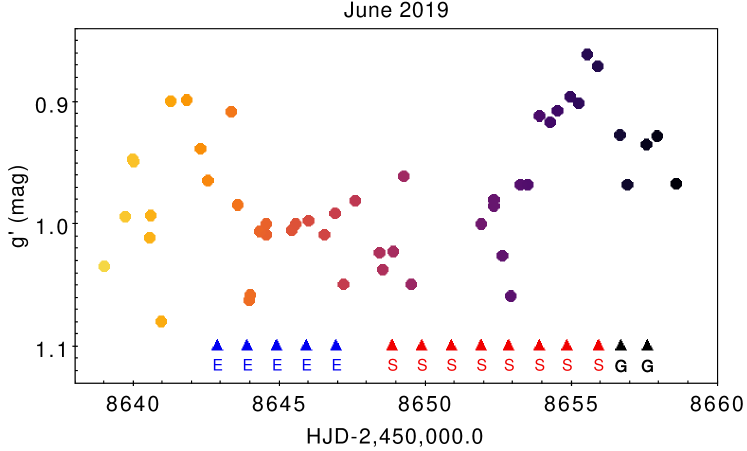
Figure 1: Visual summary of observations obtained in June 2019, as part of the DoAr 44 coordinated campaign. The differential g’-band light curve (see Section 3.2) is shown as colored circles, with the color scale reflecting the Julian Date, while the epochs of CFHT/ESPaDOnS, CFHT/SPIRou, and ESO VLTI/Gravity observations are indicated by triangles labeled with ”E”, ”S”, and ”G”, respectively. Note that the March 2019 ESPaDOnS run, which is part of the campaign reported here, is not shown in this figure. The average g-band magnitude of the system during the campaign was g=13.35 according to the publicly available Zwicky Transient Facility light curve (Masci et al., 2019).

2.1 LCOGT photomery

Photometric observations were obtained at the Las Cumbres Observatory Global Network (LCOGT, Brown et al., 2013) with the 1m Sinistro telescopes from June 4 to June 24, 2019. We used SDSS/PanSTARRS u’g’r’i’ filters with exposure times of 60, 30, 10, and 5s, respectively. A total of 219 images centered on DoAr 44 were obtained over 20 days with a cadence of nearly three photometric sequences per 24 hours. Point-spread function (PSF) photometry was performed using IRAF/DAOPHOT on the pipe-line reduced images provided by LCOGT. Over the field of view (FOV) of 27 arcmin (see Figure 2), the PSF photometry includes the target DoAr 44, the nearby W Uma eclipsing binary V2394 Oph, the T Tauri stars ROX 42B, ROX 43, ROX 47B, and DoAr 43, as well as four potential comparison and check stars: [JDH94]Oph 587, TYC 6795-600-1, TYC 6795-516-1, and an anonymous star (RA, Dec: 247.8519d, -24.3306d), referred to as C5 in the following. We verified that Oph 587 and C5, located within 10 arcmin of DoAr 44, were stable at a few 0.01 mag level in all filters. While the two TYC stars are brighter than Oph 587 and C5, and also appear to be photometrically stable at similar levels, they are located in a corner of the image, and are therefore more prone to systematics (e.g. flat-field correction).

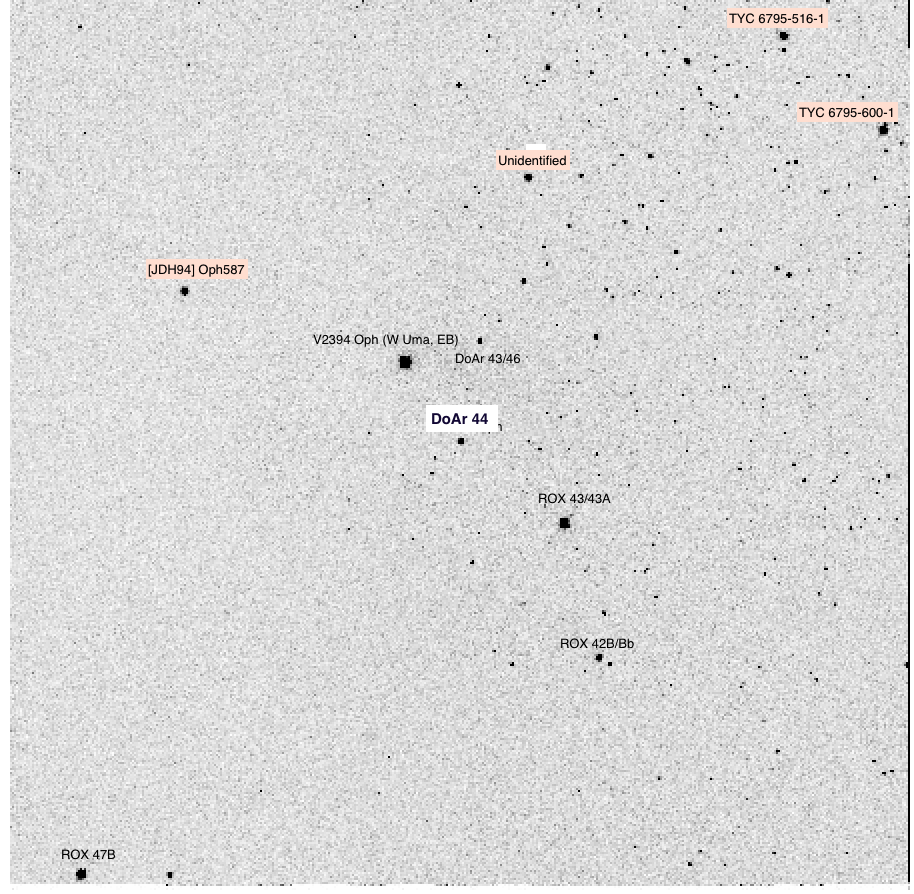
Figure 2: Field of view of LCOGT images, with the target, as well as comparison and check stars identified. North is up, east is left. The FOV is 27 arcmin on the side.

Table 1: LCOGT u’g’r’i’ differential photometry (first 10 of 229 measurements). The columns list: Julian date, differential magnitude (see text) between DoAr 44 and the comparison star, between the comparison star and the check star, filter, airmass, and Moon distance from the target. We note that the results are given for different filters on each row. In any given filter, the comparison-check star values listed in the third column are constant within errors (see text). The full table is available electronically at CDS, Strasbourg.

Julian date	Target	Check	Filt.	Airmass	Moon
(2,450,000.+)	(mag)	(mag)			dist. (°)
8638.9847732	1.03	0.39	gp	1.14	163
8638.9858978	0.09	0.28	ip	1.13	163
8638.9867561	0.5	0.43	rp	1.13	163
8638.9876614	0.95	0.02	up	1.13	163
8639.7314887	0.99	0.43	gp	1.04	152
8639.7326015	0.09	0.3	ip	1.04	152
8639.7334362	0.46	0.43	rp	1.04	152
8639.7343175	0.97	0	up	1.04	152
8639.9927617	0.94	0.4	gp	1.1	149
8639.9939326	0.06	0.3	ip	1.1	149
…

Table 2: Journal of ESPaDOnS observations of DoAr 44. All observations consist of sequences of four subexposures, each lasting 950 s. Columns respectively list, for each observation, the UT date, time, heliocentric Julian date (HJD), rotational phase, and signal-to-noise ratio (SNR) at 731 nm (per 2.6 km s^-1velocity bin).

Date	UT	HJD	$\Phi_{rot}$	SNR
(2019)	(hh:mm:ss)	(2,450,000.+)		(731nm)
Mar 15	14:31:32	8558.10852	0.48	137
Mar 16	15:32:19	8559.15082	0.83	141
Mar 18	15:11:40	8561.13665	1.50	133
Mar 19	14:47:48	8562.12015	1.83	124
Mar 20	14:13:53	8563.09667	2.16	131
Mar 21	14:50:36	8564.12225	2.51	132
Mar 22	13:32:39	8565.06818	2.83	143
Jun 08	09:16:27	8642.89230	29.12	139
Jun 09	09:21:13	8643.89558	29.46	135
Jun 10	09:19:12	8644.89415	29.80	135
Jun 11	10:15:19	8645.93308	30.15	134
Jun 12	10:07:45	8646.92779	30.48	130

Table 3: Journal of SPIRou observations of DoAr 44. All observations consist of sequences of four subexposures, each lasting 300 s. Columns respectively list, for each observation, the UT date, time, HJD, and SNR at 2135 nm per 2.3 km s^-1  velocity bin.

Date	UT	HJD	$\Phi_{rot}$	SNR
(2019)	(hh:mm:ss)	(2,450,000.+)		(2135nm)
Jun 14	08:43:03	8648.8680960	31.14	223
Jun 15	08:54:21	8649.8759002	31.48	227
Jun 16	09:17:09	8650.8916925	31.82	227
Jun 17	09:39:18	8651.9070323	32.16	137
Jun 18	08:28:37	8652.8579025	32.49	216
Jun 19	09:27:16	8653.8985925	32.84	237
Jun 20	08:07:01	8654.8428144	33.16	237
Jun 21	10:17:10	8655.9331438	33.52	211

We therefore used Oph 587 as a reference star and C5 as a check star to derive the differential light curves for DoAr 44. Stars Oph 587 and C5 are within one magnitude of difference from the target’s brightness in all filters. The rms error of the photometric measurement in each filter amounts to about 0.02 mag. DoAr 44 is found to be variable in all four filters: the rms dispersion of the u’g’r’i’ differential light curves (DoAr 44 - Oph 587) is 0.17, 0.09, 0.07, and 0.09 mag, respectively, while the corresponding values for the comparison and check stars (Oph 587 - C5) are 0.03, 0.03, 0.04, and 0.04 mag. The nearby bright Moon toward the middle of the photometric campaign (June 16, 2019; JD 2458650.5) strongly increased the sky background, especially in the u’-band, leading to poorer quality photometry around this date. DoAr 44’s differential photometry is provided in Table 1.

2.2 CFHT spectropolarimetry

Optical spectropolarimetric observations of DoAr 44 were completed during two runs, from March 15 to 22 and from June 8 to 12, 2019, with the ESPaDOnS spectropolarimeter at the Canada-France-Hawaii Telescope (CFHT), at a resolving power of 65,000 covering 370 to 1,000 nm (Donati, 2003). During the first run, seven circularly polarized spectra were collected, and five additional spectra were obtained during the second run. Raw frames were reduced with the standard ESPaDOnS reduction package, and a least-squares deconvolution (LSD, Donati et al., 1997) was applied to all spectra, using a line list appropriate to DoAr 44. The journal of observations is presented in Table 2. Near-IR spectropolarimetric observations of DoAr 44 were completed from June 14 to 21, 2019 with the SPIRou spectropolarimeter at the CFHT, covering from 0.95 to 2.50 microns, at a spectral resolution of 70,000 (Donati et al., 2020) at a rate of one visit per night. Raw data were processed by the SPIRou pipe-line at CFHT and the reduced data provided by the Canadian Astronomy Data Center. The journal of observations is presented in Table 3.

Table 4: Stellar properties of the DoAr 44 system. The V-band and 2MASS J-band magnitudes, and the Gaia DR2 distance are taken from the literature (see text). All other values are derived in this study.

V, J	12.6, 9.1
SpT	K2-K3
AV	2.0$\pm$0.2 mag
$T_{\rm eff}$	4600$\pm$120 K
${\rm L}_{\star}$/${\rm L}_{\odot}$	1.6$\pm$0.2
${\rm R}_{\star}$/${\rm R}_{\odot}$	2.0$\pm$0.15
${\rm M}_{\star}$/${\rm M}_{\odot}$	1.2$\pm$0.15
EW(LiI)	430 mÅ
$v\sin i$	17.0$\pm$1.1 km s-1
${\rm P}_{rot}$	2.960$\pm$0.018 d
$i$	30$\pm$5 °
$\dot{M}_{\rm acc}$	7$\pm$3 10-9 ${\rm M}_{\odot}{\rm yr}^{-1}$
$d$	146$\pm$1 pc
$r_{cor}$	0.043 au (4.63 ${\rm R}_{\star}$)
$r_{sub}$	0.044 au (4.74${\rm R}_{\star}$)

2.3 ESO/VLTI interferometry

DoAr 44 was observed on June 22 and 23, 2019 in the K-band with the GRAVITY instrument (Gravity Collaboration et al., 2017) combining the four unit telescopes of the ESO/VLTI (ESO run 60.A-9256). At 2.2 $\mu$m, with a maximum baseline of 130 m, we thus reach an angular resolution of $\lambda$/2Bmax = 1.7 mas, corresponding to 0.25 au at 146 pc. We used the instrument in its high spectral-resolution mode (R $\sim$ 4000), thus partly resolving the ${\rm Br}\gamma$ line profile. The observations, data reduction, and interferometric results are described in full in Paper I.

3 Results

3.1 Stellar properties

We derived estimates of the system’s properties based on the newly acquired high-resolution spectra. We followed the same procedure as we used in Pouilly et al. (2020) to which the reader is referred for details. We selected 16 spectral windows between 600 and 800 nm where the mean ESPaDOnS spectrum of DoAr 44 is fit with a synthetic spectrum generated from the ZEEMAN code (Folsom et al., 2012) based on MARCS stellar atmosphere grids (Gustafsson et al., 2008) and VALD line lists (Ryabchikova et al., 2015). Assuming $\log g$= 4.0, we derived the following parameters: $v\sin i$= 17.0 $\pm$ 1.1 km/s, ${\rm V}_{r}$= -5.70 $\pm$ 0.24 km/s, $T_{\rm eff}$= 4600 $\pm$ 120 K, and ${\rm V}_{mic}$= 0.27 $\pm$ 0.27 km s^-1. The veiling, that is to say, the ratio of the continuum excess flux to the stellar photospheric flux, is measured as constant over time and amounts to $r\simeq$0.18$\pm$0.05 over the wavelength range 610-670 nm.

Using the optical photometry of Bouvier et al. (1988) and 2MASS J-band, and adopting a K2-K3 spectral type with intrinsic colors listed in Pecaut & Mamajek (2013), we derived color excesses in the (V-I_c) and (V-J) colors that correspond to a visual extinction A_V=2.0$\pm$0.2 mag. From the J-band magnitude, bolometric corrections from Pecaut & Mamajek (2013) for K2-K3 young stars, and a distance of 146$\pm$1 pc (Gaia Collaboration et al., 2016, 2018), we thus obtained ${\rm L}_{\star}$=1.6$\pm$0.2 ${\rm L}_{\odot}$. Combined with $T_{\rm eff}$=4600 K derived above, this yields ${\rm R}_{\star}$=2.0$\pm$0.15 ${\rm R}_{\odot}$. From its position in the HR diagram, we derived ${\rm M}_{\star}$=1.23$\pm$0.15 ${\rm M}_{\odot}$ using the CESAM evolutionary models (Marques et al., 2013), and the star appears to have a modest radiative core, with M_rad/${\rm M}_{\star}$=0.22$\pm$0.20 and R_rad/${\rm R}_{\star}$=0.35$\pm$0.2, where M_rad and R_rad are the mass and radius of the radiative core, respectively. We note, however, that the latter values are strongly model dependent, as, using Siess et al. (2000) models, we would derive ${\rm M}_{\star}$=1.4 ${\rm M}_{\odot}$, M_rad/${\rm M}_{\star}$=0.73 and R_rad/${\rm R}_{\star}$=0.50.

Finally, we used the above estimate of the stellar radius to derive the inclination of the stellar rotational axis on the line of sight (LoS). Using $v\sin i$=17 km s^-1 and ${\rm P}_{rot}$=2.96 d (see below), and propagating the uncertainties, yields $\sin i$=0.50$\pm$0.05, which translates to $i$=30$\pm$5°, meaning the system is seen at low inclination. Table 4 summarizes the properties of the stellar system with their uncertainties.

3.2 Photometric variability

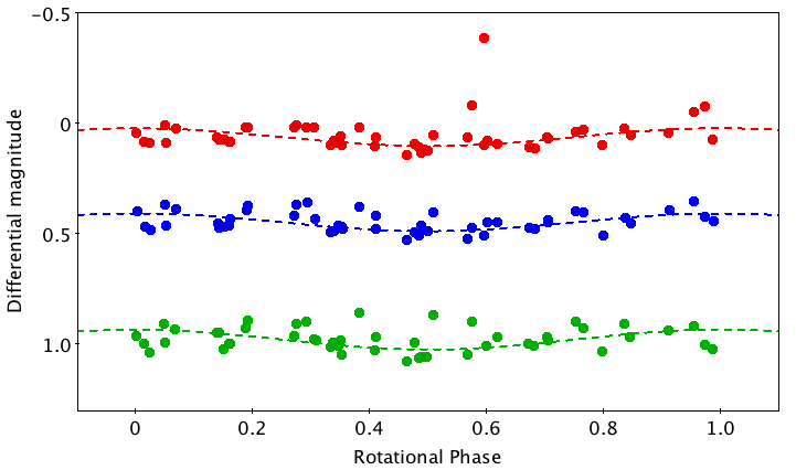
Figure 3: DoAr 44 photometric variations. The g’r’i’ light curves (green, blue, and red, respectively) are shown folded in phase with a period of 2.960 days derived from periodogram analysis (see text). A sine curve was eye fit to the light curves and is shown for illustration with a peak-to-peak amplitude of 0.08 mag in the g’r’i’ bands.

The LCOGT observations yielded 20 day-long differential light curves for DoAr 44 in the u’g’r’i’ filters. We searched for a periodicity in the photometric variations, excluding about five measurements per filter taken when the bright moon was under 15 degrees away from the target. We used both the CLEAN periodogram analysis (Roberts et al., 1987) and the string-length method (Dworetsky, 1983). The former yields a period of 3.09 d in the r’ filter only, while the latter returns a most probable period in all filters in the range from 2.97 d to 3.07 d. In order to confirm the period, we downloaded ASAS-SN photometry (Shappee et al., 2014), which contains 288 single filter measurements over a single season extending from MJD 57780 to MJD 58030 (February-September 2017). Using the same period-search algorithms, we found a clear periodicity of 2.960 +/- 0.018 d in this much richer dataset, with a peak-to-peak amplitude of about 0.1 mag. The LCOGT g’r’i’ light curves folded in phase with this period are shown in Fig. 3 and suggest a low-level modulation by surface spots, of the order of a 0.08 mag peak to peak in the g’r’i’ filters. While a period is found in the u’-band light curve as well, the phased light curve exhibits a scatter of the same order as the photometric amplitude. We therefore adopted the more accurate 2.960 d period derived from the ASAS-SN dataset and ascribed it to the rotational period of the star. We thus define an ephemeris such that the origin of phase corresponds to the epoch of maximum brightness at the time of our observations, so

$$HJD(d)=2,458,556.7+2.960\times E.$$ (1)

Finally, we note that the uncertainty on the derived period, $\delta$P=0.018d, could induce a phase shift between the March and June ESPaDOnS runs up to $\delta\Phi$=0.16 rms.

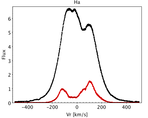
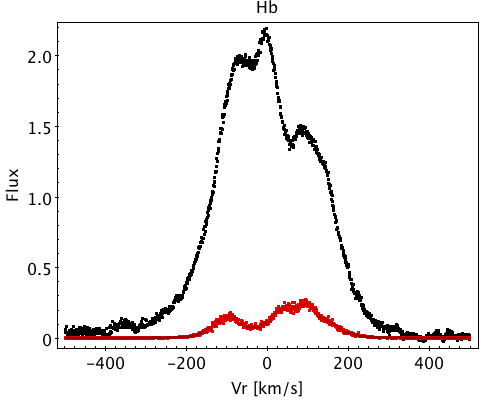
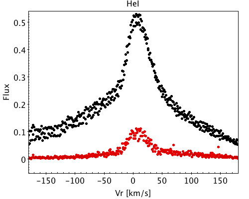
Figure 4: From left to right: mean (black) and variance (red) residual profiles for ${\rm H}\alpha$, ${\rm H}\beta$, and ${\rm HeI}$ 587.6 nm. ${\rm H}\alpha$ and ${\rm H}\beta$ appear on overlapping spectral orders, which are both shown here. For ${\rm HeI}$, the variance has been multiplied by 10. The increased scatter over the blue wing of the ${\rm HeI}$ line profile is due to spectral order overlap.

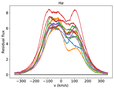
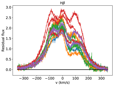
Figure 5: Superimposed residual line profiles: H$\alpha$ (left) and H$\beta$ (right). The color code corresponds to different rotational cycles. Each line is covered by two spectral orders and both are shown.

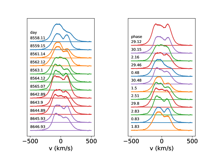
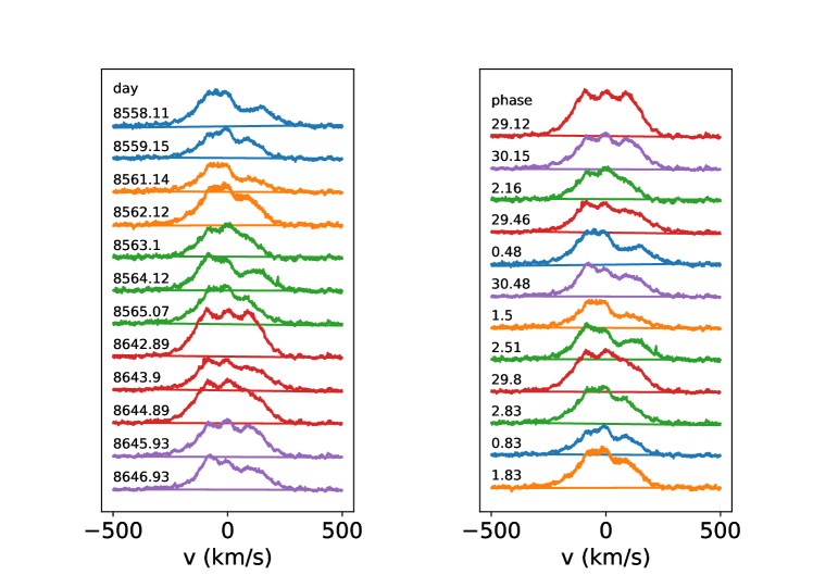
Figure 6: H$\alpha$ (top) and H$\beta$ (bottom) residual line profile variability as a function of date and phase. The color code corresponds to different rotational cycles. We note that both profiles appear less asymmetric in June than in March 2019, with a more depressed red wing at the earlier epoch.

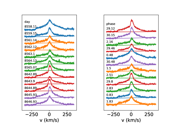
Figure 7: Same as Fig. 6 for HeI 587.6 nm residual line profile. We note the presence of a narrow component superimposed on a broad pedestal. Similar line profiles are observed in March and June 2019.

Table 5: Photospheric radial velocity, ${\rm V}_{r}$, and equivalent width, W, of ${\rm H}\alpha$, ${\rm H}\beta$, and ${\rm HeI}$ emission lines from ESPaDOnS spectra.

HJD	${\rm V}_{r}$†	W(${\rm H}\alpha$)	W(${\rm H}\beta$)	W(${\rm HeI}$)
(-2,450,000)	km s-1	(Å)	(Å)	(Å)
8558.10852	-5.59	41.6	8.2	1.13
8559.15082	-5.78	38.2	5.8	0.62
8561.13665	-5.60	31.8	4.3	0.60
8562.12015	-5.80	48.1	7.7	0.85
8563.09667	-6.00	41.0	5.8	0.46
8564.12225	-5.63	44.1	6.8	0.76
8565.06818	-5.76	45.5	7.2	0.80
8642.89230	-6.10	60.5	12.5	1.06
8643.89558	-5.55	44.8	6.6	0.66
8644.89415	-5.66	53.3	10.0	1.04
8645.93308	-6.02	43.9	7.7	0.99
8646.92779	-5.58	39.6	6.1	0.77

^† The rms uncertainty on ${\rm V}_{r}$ amounts to 0.05 km/s.

3.3 Optical line profiles

Deciphering the shape and variability of the emission line profiles seen in the spectra of cTTSs offers a window to the physical processes occurring close to the star, particularly the structure and dynamics of accretion and outflows (e.g., Alencar & Basri, 2000; Edwards et al., 2006; Lima et al., 2010; Esau et al., 2014). In the optical range, DoAr 44’s spectrum shows line emission primarily the HI Balmer and Paschen series, in the CaII H&K doublet and near-IR triplet, as well as in the ${\rm HeI}$ 587.6 nm, 667.8 nm, and 706.6 nm, [OI] 630.0 nm, and OI 777.3 nm lines. Residual emission line profiles were computed by subtracting the broadened photospheric spectrum of the Hyades cluster member Melotte 25-151, a K2-type star with ${\rm V}_{r}$= 37.98 km s^-1, $v\sin i$= 4.83 km s^-1, and $T_{\rm eff}$= 4920 K (Folsom et al., 2018), also observed with ESPaDOnS.

3.3.1 Line profile variability

The spectral series we obtained on DoAr 44 with CFHT/ESPaDOnS allows us to investigate the spectral variability of the source on timescales ranging from days to months. Figure 4 shows the mean and variance profile for the main emission lines. The Balmer line profiles are double peaked with a slightly depressed red peak, corresponding to the Type II(R) profiles in the classification of Reipurth et al. (1996). This profile shape is qualitatively accounted for by dipolar magnetospheric accretion models considering moderate to low inclinations, $i\simeq 30-45\degr$ (Muzerolle et al., 1998, 2001). Both the ${\rm H}\alpha$ and ${\rm H}\beta$ profiles exhibit significant variance in the blue and red wings up to velocities of a few hundred km s^-1, and comparatively less variability in the line center. As is often observed in T Tauri stars (Beristain et al., 2001), the ${\rm HeI}$ line profile is composite, consisting of a centrally peaked broad component, extending up to velocities of $\pm$200 km s^-1, and a narrow component located close to the line center with a FWHM of about 40 km s^-1. The profile’s variability seems to be predominantly associated with the narrow component. According to Beristain et al. (2001), the properties of this type of ${\rm HeI}$ profile suggest the narrow component arises in the post-shock region close to the stellar surface, while the broad component is formed in the main accretion column above the accretion shock.

Figure 5 shows the superimposed H$\alpha$ and H$\beta$ line profiles recorded for DoAr 44 during the CFHT/ESPaDOnS runs of March and June 2019. Figure 6 is another representation of the same dataset, ordered by Julian date and by rotational phase. Similar plots are shown for the HeI 587.6 nm line in Fig. 7. We note that the Balmer line profiles appear more symmetric in June than in March, while the ${\rm HeI}$ line profile has remained the same, and it exhibits a broad component and a narrow component at both epochs. Remarkably, the ${\rm H}\alpha$ and ${\rm H}\beta$ profiles do no exhibit high-velocity redshifted absorptions below the continuum at any rotational phase, contrary to what is often seen in other accreting sources as the funnel flow intercepts the LoS (e.g., Bouvier et al., 2007a; Alencar et al., 2012, 2018). The lack of inverse P Cygni profile signatures provides further support for a low inclination of the system (Muzerolle et al., 2001), as independently derived for the stellar rotational axis and for the outer disk that both suggest $i\simeq$20-35°(see above and Paper I).

Equivalent width measurements for ${\rm H}\alpha$, ${\rm H}\beta$, and ${\rm HeI}$ emission lines are reported in Table 5. As the continuum is well defined around these lines, the equivalent width measurement is accurate to within a few percent. The median equivalent widths over the two epochs amount to 44, 6.8, and 0.8 Å, for ${\rm H}\alpha$, ${\rm H}\beta$, and ${\rm HeI}$ lines, respectively. The lines have slightly larger median equivalent widths in June than in March. Their variation as a function of rotational phase is shown in Fig. 8. There is a hint of rotational modulation in the equivalent width variations of the three line profiles during the June run, with minimum values close to a rotational phase of 0.5, while no such modulation is seen in the March run. We estimate the mass accretion rate onto the star from the flux measured in the ${\rm H}\alpha$ and ${\rm H}\beta$ lines, using relationships between accretion and line luminosity from Alcalá et al. (2014). From the ${\rm H}\alpha$ line we thus derive $L_{\rm acc}$/${\rm L}_{\odot}$=0.06-0.13, taking into account $EW({\rm H}\alpha$) variations, which yields $\dot{M}_{\rm acc}$=4.0-8.5 10^-9 ${\rm M}_{\odot}{\rm yr}^{-1}$ assuming a magnetospheric truncation radius of 5 ${\rm R}_{\star}$. Similarly, from the ${\rm H}\beta$ line, we obtain $L_{\rm acc}$/${\rm L}_{\odot}$=0.05-0.17 and $\dot{M}_{\rm acc}$=3-10 10^-9 ${\rm M}_{\odot}{\rm yr}^{-1}$. These estimates are consistent with those reported by Manara et al. (2014), who obtained $\dot{M}_{\rm acc}$=6.3 10^-9 ${\rm M}_{\odot}{\rm yr}^{-1}$  from slab models applied to XSHOOTER spectra.

A periodogram analysis of the line profiles is detailed in Appendix A. The analysis does not reveal any significant periodicity in the intensity variations of the velocity channels across the ${\rm H}\alpha$, ${\rm H}\beta$, and ${\rm HeI}$ line profiles when the full dataset is analyzed. This presumably results from the large temporal gap between the March and June ESPaDOnS runs. As described in Appendix A, when each run is analyzed independently, we do find some evidence for the rotational modulation of the ${\rm H}\alpha$ and ${\rm H}\beta$ line profiles at the stellar rotation period. More specifically, the intensity of the red wing (from about +50 to +150 km s^-1) of the ${\rm H}\alpha$ and ${\rm H}\beta$ profiles appears to be modulated at the stellar rotation period during the March run. Since the veiling is nearly constant at these dates, we ascribe these variations to changes in the intrinsic line flux, as opposed to continuum variations. This result is of limited significance, due to the poor rotational phase sampling and the low number of spectra obtained during each run. Nevertheless, the examination of the shape of the line profiles plotted as a function of rotational phase in Fig. 20 tends to support rotational modulation at both epochs, with a systematically depressed line flux in the red part of the profile around phase 0.5 for Balmer lines, as expected from accretion funnel flows as they cross the LoS (e.g., Symington et al., 2005).

3.3.2 Line profile decomposition

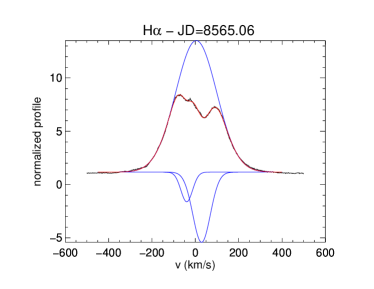
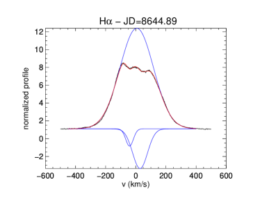
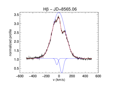
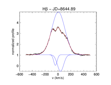
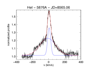
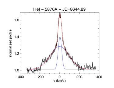
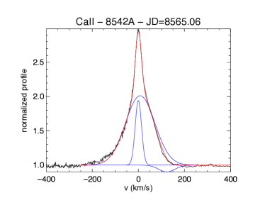
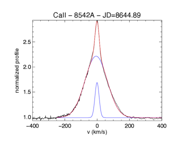
Figure 23: Line profile decomposition in Gaussian components. The Gaussian components are shown as blue curves, and the resulting modeled profile in red, while the observed profile is in black. From top to bottom: ${\rm H}\alpha$, ${\rm H}\beta$, ${\rm HeI}$, and Ca II 854.2 nm.

We further analyzed the line profiles attempting to reproduce their shape as a combination of Gaussian components. Details on the line profile decomposition are given in Appendix B, and a few examples are illustrated in Fig. 23. The Balmer line profiles are well fit with three Gaussian components, consisting of a broad central emission peak and two absorption components, one blueshifted, and the other redshifted, relative to the line center. The ${\rm HeI}$ line profile can be reproduced using only two emission components, a broad and a narrow one. The results are given in Table 8, which lists the equivalent width, peak intensity, radial velocity, and FWHM of each component.

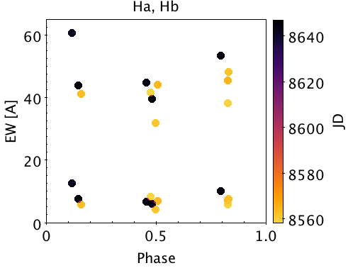
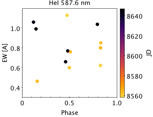
Figure 8: Equivalent width (Å) as a function of rotational phase. Left panel: ${\rm H}\alpha$ (top) and ${\rm H}\beta$ (bottom); right panel: ${\rm HeI}$. The color code corresponds to Julian date, mostly March (bright) and June (dark) 2019.

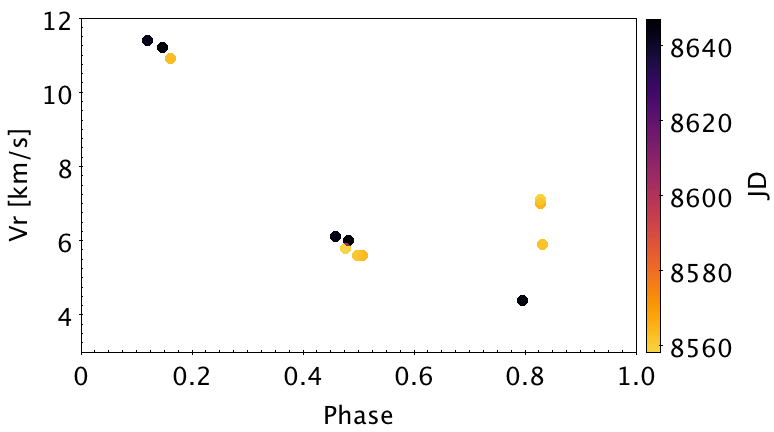
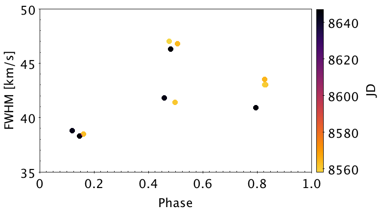
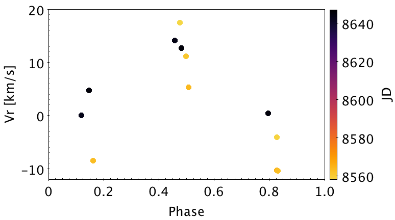
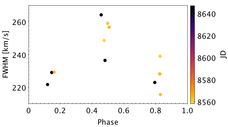
Figure 9: Radial velocity (left) and FWHM (right) variations of the narrow (top) and broad (bottom) components of the ${\rm HeI}$ line profile in the stellar rest frame as a function of rotational phase. The color code reflects the Julian date for the March (bright) and June (dark) ESPaDOnS runs.

The narrow component of the ${\rm HeI}$ line profile shows significant radial velocity variations between +4.4 and +11.4 km s^-1 in the stellar rest frame, while its FWHM varies over the range 38-47 km s^-1. We find these variations to be modulated by stellar rotation with a strong phase coherence between the March and June ESPaDOnS runs (see Figure 9). Assuming that the ${\rm HeI}$ line narrow component arises from the accretion post-shock (Beristain et al. 2001), as suggested by its slightly redshifted velocity, and covers a small area on the stellar surface, one can relate the radial velocity amplitude $\delta$${\rm V}_{r}$ to the hot spot latitude $\theta$, with $\delta V_{r}=2\cdot$$v\sin i$$\cdot\cos\theta$ (Bouvier et al., 2007a). We deduce a latitude of 78$\pm$2^∘ for the accretion shock at the stellar surface, assuming an uncertainty of 0.5 km s^-1 on $\delta$${\rm V}_{r}$.

Interestingly, the radial velocity of the wide component of the ${\rm HeI}$ line profile seems to be rotationally modulated as well, albeit with increased scatter. If this component arises from a hot wind close to the star, the modulation may result from the geometric projection of the wind velocity pattern onto the LoS. However, its slightly redshifted velocity relative to the star instead suggests it arises from the accretion funnel flow, located above the post-shock region probed by the narrow component (Beristain et al., 2001). The FWHM of the narrow and wide components appears to be rotationally modulated as well. They reach a maximum at phase 0.5 of 259 km s^-1 for the broad component and 47 km s^-1 for the narrow one, and both vary by about 15% along the rotational cycle. This variation could conceivably be related to the projection on the LoS of the velocity gradients of the emitting regions responsible for the narrow and broad ${\rm HeI}$ components. The vastly different FWHM of the narrow and broad components, and the fact that the radial velocities of both components appear to be modulated but reach a maximum value at different rotational phases (see Fig. 9), suggest the two components probe different regions along the funnel flow.

Considering the two absorption components in the ${\rm H}\alpha$ profile, one being blueshifted, the other redshifted, we find that their FWHMs are rotationally modulated and strongly anti-correlated (see Table 8). The equivalent width and peak absorption intensity of the blueshifted component are the largest around phase 0, while the equivalent width of the redshifted absorption component is the largest around phase 0.5. As the former is probably related to an outflow, while the latter probes accretion, this suggests that both flows are physically related and occur at opposite rotational phases. We also notice a hint of a correlation between the radial velocity variations of these two absorption components in the ${\rm H}\alpha$ line profile, as reported earlier for AA Tau (Bouvier et al., 2003) and LkCa 15 (Alencar et al., 2018).

As illustrated in Fig. 23, the decomposition of the CaII 854.2 nm emission line reveals the presence of a highly redshifted absorption component during the March run, around ${\rm V}_{r}$$\simeq$+120 km s^-1. It is observed at phases 0.83 (JD 8559.15) and 2.83 (JD 8565.07), but, surprisingly enough, not at phase 1.83 (JD 8562.12). Similar high-velocity redshifted absorptions are also seen in the NaI D line profiles at the same phases. This suggests transient accretion episodes onto the stellar surface or, at least, mass accretion rate variations occur within the funnel flow. No redshifted absorption components are seen in this line profile during the June run.

3.3.3 Correlation matrices

The observed emission lines of DoAr 44 are highly variable, with emission and absorption components superposed, as can be seen in Fig 5. The different components may come from various circumstellar regions, like the chromosphere, the accretion funnel, and the wind, which can vary over different timescales. To investigate how the variations across a line or between different lines are related, we calculated correlation matrices consisting of 2D plots of the linear correlation coefficients of the line profile intensity variations at different velocity bins. A good correlation between two components indicates a common origin of the components, for example.

The H$\alpha$ and H$\beta$ lines are similar, and their correlation matrices also show the same characteristics (Fig. 10). There is little correlation between the blue and red part of the profile, which suggests different physical processes at the origin of their variability. The red wing of the profile varies coherently beyond +200 km s^-1 and is strongly anti-correlated with the red emission peak around 100 km s^-1. This red emission peak is strongly variable, as can be clearly seen in Figs. 5 and 6. As the velocity channels corresponding to the peak appear to be modulated at the stellar rotation period, we interpret its anti-correlation with the profile’s far red wing as the signature of periodic redshifted absorptions due to the funnel flow crossing the LoS.

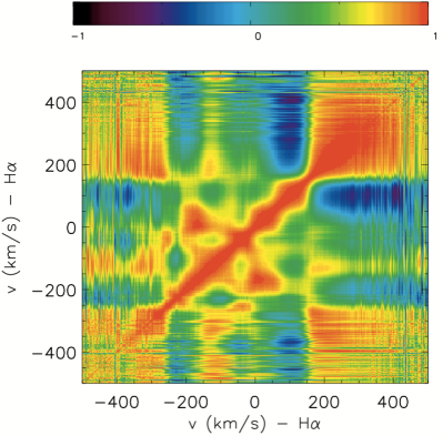
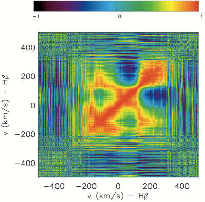
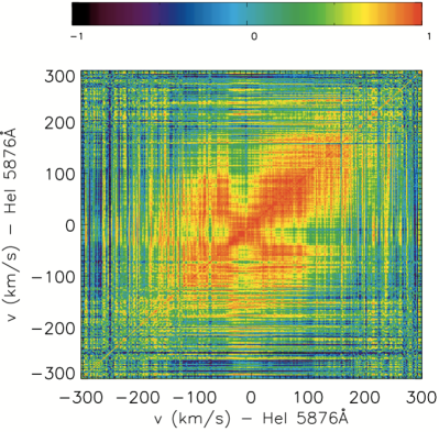
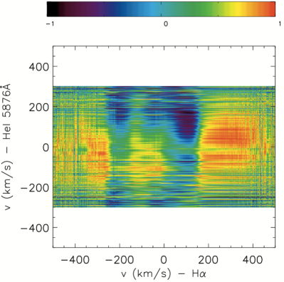
Figure 10: Top: auto-correlation matrices of ${\rm H}\alpha$ (left) and ${\rm H}\beta$ (right) line profile variation for ESPaDOnS March run. Bottom: auto-correlation matrices of ${\rm HeI}$ (left) and cross-correlation matrices of ${\rm HeI}$ vs. ${\rm H}\alpha$ (right).

The ${\rm HeI}$ line is composed of a broad and a narrow component. The correlation matrix is shown in Fig. 10. It indicates that the BC varies coherently and independently of the NC component. The ${\rm H}\alpha$ vs. ${\rm HeI}$ cross correlation matrix reveals that the ${\rm HeI}$ BC component is correlated with the high velocity wings of the Balmer profile beyond 200 km s^-1. The red wing of the ${\rm HeI}$ BC is, however, strongly anti-correlated with the red emission peak seen in the ${\rm H}\alpha$ profile around 100 km s^-1. This suggests that redshifted absorption in the ${\rm H}\alpha$ profile occurs as the BC of the ${\rm HeI}$ line profile becomes stronger, which is consistent with both the redshifted ${\rm H}\alpha$ absorption and the ${\rm HeI}$ BC emission originating from an accretion funnel flow crossing the LoS.

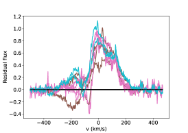
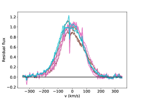
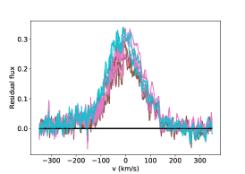
Figure 11: HeI 1083.3 nm (left), ${\rm Pa}\beta$ (middle), and ${\rm Br}\gamma$  (right) residual line profiles. The narrow, slightly blueshifted absorption component close the center of the ${\rm Pa}\beta$ line profile is due to imperfect telluric line correction. The color code corresponds to successive rotational cycles.

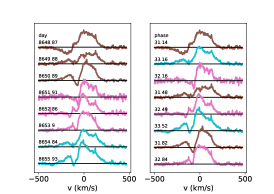
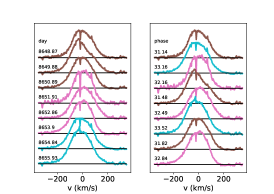
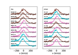
Figure 12: HeI 1083.3 nm (left), ${\rm Pa}\beta$ (middle), and ${\rm Br}\gamma$  (right) residual line profile variability as a function of date and phase. The narrow, slightly blueshifted absorption component close to the center of the ${\rm Pa}\beta$ line profile is due to imperfect telluric line correction. The color code corresponds to different rotational cycles.

3.4 Infrared line profiles

Table 6: Equivalent width (EW) of ${\rm HeI}$ 1083.3 nm, ${\rm Br}\gamma$, and ${\rm Pa}\beta$ emission lines from SPIRou spectra. The uncertainty on EW is of the order of 0.1-0.2 Å depending on the SNR.

HJD	EW(${\rm HeI}$)	EW(${\rm Br}\gamma$)	EW(${\rm Pa}\beta$)
(-2,450,000)	(Å)	(Å)	(Å)
8648.86809	4.0	2.7	6.9
8649.87590	4.7	3.0	8.6
8650.89169	5.5	3.2	8.4
8651.90703	4.0	3.4	8.1
8652.85790	5.1	2.8	8.6
8653.89859	6.8	3.3	8.5
8654.84281	6.7	3.8	8.9
8655.93314	8.3	4.0	9.3

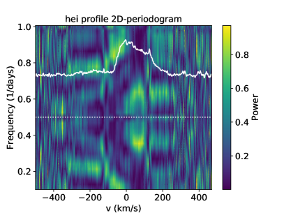
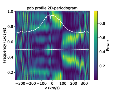
Figure 13: 2D periodogram of the ${\rm HeI}$ 1083.3 nm (left) and ${\rm Pa}\beta$ (right) line profiles computed from the eight SPIRou spectra obtained on consecutive nights. The color code represents the periodogram power, and the superimposed white curve is the average line profile. We note the symmetry of the periodogram around the frequency 0.5 d^-1 due to the one-day alias resulting from the night-to- night sampling.

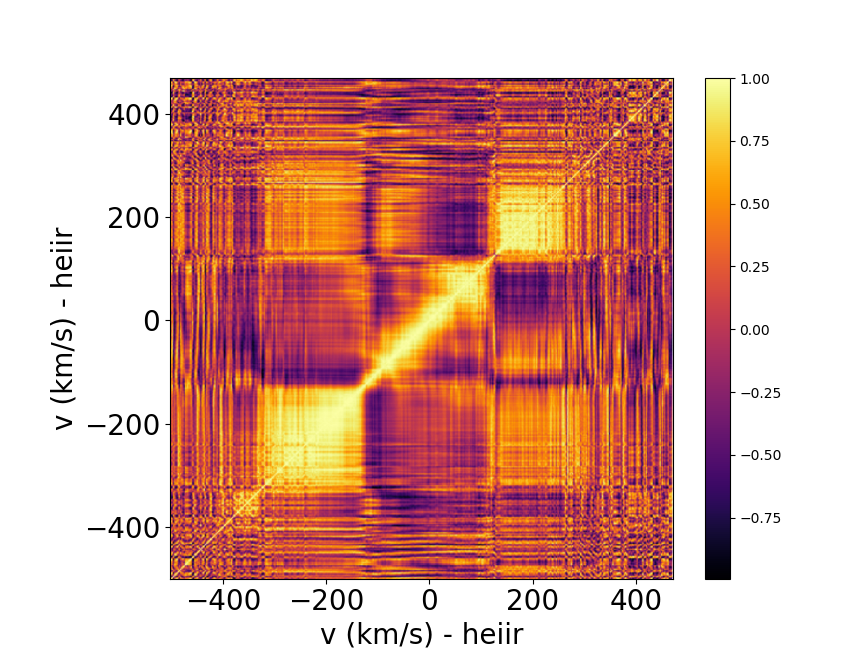
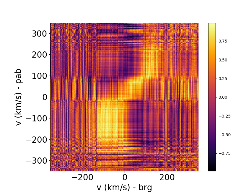
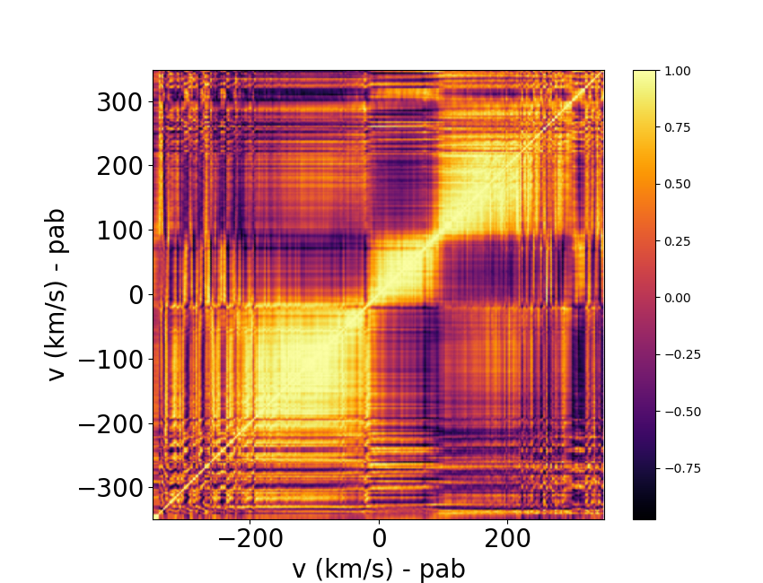
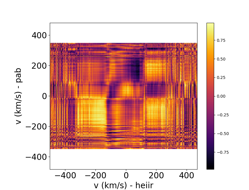
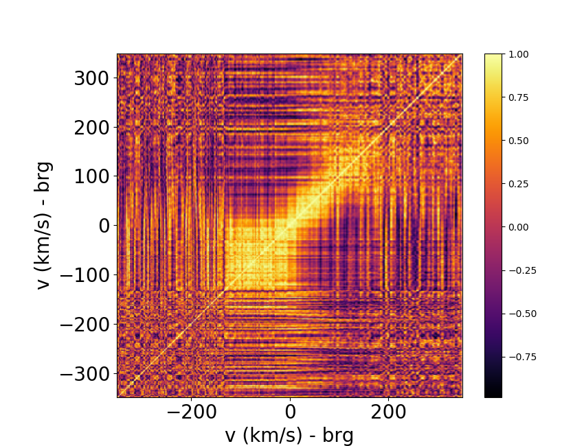
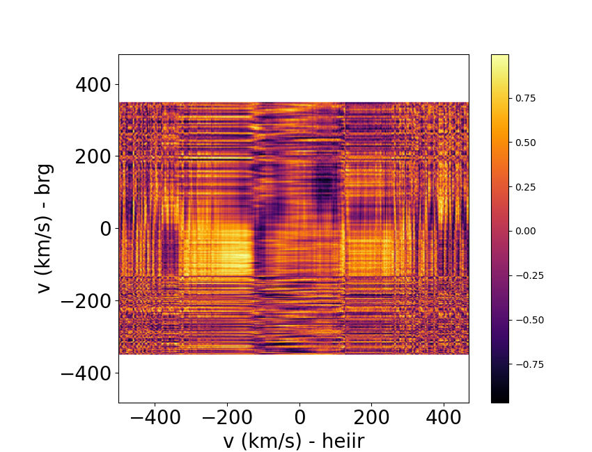
Figure 14: Auto-correlation matrices for the ${\rm HeI}$, ${\rm Pa}\beta$, and ${\rm Br}\gamma$  line profiles (left), and cross-correlation matrices for the three line profiles (right).

The wide spectral range covered by SPIRou includes a number of circumstellar diagnostics, such as ${\rm HeI}$ 1083.3 nm, ${\rm Pa}\beta$ 1282.2 nm, and ${\rm Br}\gamma$ 2166.1 nm. These lines are seen in emission in all the spectra acquired during the SPIRou observing run, and their equivalent widths are listed in Table 6. From the equivalent widths of the ${\rm Pa}\beta$ and ${\rm Br}\gamma$ line profiles measured on the mean spectrum, EW(${\rm Pa}\beta$) = 8.75 $\pm$ 0.15 Å and EW(${\rm Br}\gamma$) = 3.5 $\pm$ 0.2 Å, and using Alcalá et al. (2014) relationship between line and accretion luminosities, we derived a mass accretion rate $\dot{M}_{\rm acc}$= 6.5 $\pm$ 0.5 10^-9 ${\rm M}_{\odot}{\rm yr}^{-1}$, which is consistent with the estimate obtained above from the luminosity of the optical emission lines.

Residual line profiles were computed following the same procedure as described above for optical spectra, using the weak-line T Tauri star V819 Tau (SpT K4) as a template, also observed with SPIRou. Line profiles are shown in Figure 11. The ${\rm HeI}$ profile exhibits a strongly asymmetric shape, with significant blueshifted absorption components reaching down to velocities of -350 km s^-1  with a depth that varies on a timescale of days, while the red wing appears in emission and also exhibits significant variability. In contrast, the ${\rm Pa}\beta$ and ${\rm Br}\gamma$ profiles are much more symmetric, with only low-level variability in intensity over the course of the observations. The profiles are plotted as a function of date and rotational phase in Fig. 12.

We performed a 2D periodogram analysis across the line profiles. The 2D periodogram of the ${\rm Pa}\beta$ line profile is shown in Fig. 13. A strong signal appears at the star’s rotational period in the redshifted wing of the profile over a velocity range extending from +100 to +200 km s^-1. Radiative transfer models of magnetospheric accretion onto an inclined dipole (e.g., Kurosawa et al., 2008) predict such a rotationally modulated intensity of the high velocity redshifted wing of the ${\rm Pa}\beta$ profile, as funnel flows periodically cross the LoS. A strong signal is also seen in the 2D periodogram from the line center up to +100 km s^-1 at frequencies around 0.9 d^-1, with its alias at 0.1 d^-1. The former frequency is close to the sampling rate, and the latter is beyond the observation time span. The signal at these frequencies is therefore probably spurious, being induced by the observing window. Nevertheless, the variability seen in this part of the ${\rm Pa}\beta$ profile is real, and is also seen in the ${\rm Br}\gamma$ line profile over the same velocity channels, where the line intensity seems to first increase then decrease smoothly over the time span of the observations (see Fig. 11).

The 2D periodogram of the ${\rm HeI}$ line profile displays the strongest signal at a frequency corresponding to the stellar rotation period, extending over redshifted velocity channels from +30 to +100 km s^-1  (see Fig. 13). This periodic variability of the red part of the line profile is most likely induced by the rotational modulation of accretion funnel flow as the star rotates (e.g., Fischer et al., 2008). The other parts of the ${\rm HeI}$ profile are extremely variable, especially around the line center and throughout the blueshifted wing down to velocities of -350 km s^-1. The blue wing exhibits a rapidly changing blueshifted absorption component sometimes reaching below the continuum. Yet, this outflow component shows no sign of modulation. Instead, we observe significant change in ${\rm HeI}$ line profiles taken at the same rotational phase over successive cycles, for example, at $\phi$=31.14, 32.16, 33.16, and at $\phi$=31.48, 32.49 (see Fig. 12), which suggests intrinsic variations of the outflow component over a timescale of days. The velocity of the peak of the blueshifted absorption component appears to be the most extreme at the beginning of the observations (v${}_{blue}\simeq$ -200 km s^-1), shifting toward the line center up to v${}_{blue}\simeq$ -60 km s^-1  within three days, then returning to much bluer channels ($v_{blue}\simeq$ -130 km s^-1) over the same timescale. Its width changes as well, the most blueshifted absorption having the largest FWHM.

Radiative transfer models assign the presence of moderately blueshifted, narrow absorption components in the profile of the ${\rm HeI}$ 1083.3 nm line to a disk wind (e.g., Kurosawa et al., 2011), while broader absorptions extending to large blueshifted velocities are usually considered as the signature of accretion powered, hot inner winds originating close to the star (e.g., Edwards et al., 2003, 2006). We are apparently witnessing here a mix of disk and “stellar” winds, with a predominance of the former except for the first spectrum of the series, whose relative strength varies on a timescale of days.

Indeed, the gallery of emission line profiles gathered from the quasi-simultaneous optical and near-IR high-resolution spectra obtained for DoAr 44 during this campaign, including ${\rm HeI}$ 587.6 nm, ${\rm HeI}$ 1083.3 nm, ${\rm H}\alpha$, ${\rm H}\beta$, ${\rm Pa}\beta$, and ${\rm Br}\gamma$, bears strong resemblance with synthetic line profiles derived from the combined magnetospheric accretion and disk wind, low-inclination (i=20$\degr$) model presented in Fig.7 of Kurosawa et al. (2011). It is therefore likely that most of the emission seen in these profiles comes from magnetospheric funnel flows controlled by a misaligned dipole, with additional wind components best seen in the ${\rm HeI}$ near-IR line profile. The qualitative agreement between observations and models supports this interpretation. The low inclination of the system is further supported by the maximum edge velocity at which the blueshifted ${\rm HeI}$ absorption component meets the continuum, which amounts to -350 km s^-1. According to the edge velocity versus the system’s inclination relationship reported for this component by Appenzeller & Bertout (2013), here the system’s inclination should lie in the range 20-35$\degr$.

The auto-correlation matrices of the three profiles are shown in Fig. 14 and share the same behavior: different parts of the line profile vary independently of each other. In the ${\rm Pa}\beta$ line for instance, the blue wing varies independently of both the low-velocity and high-velocity redshifted channels, and the latter also varies independently. The cross-correlation matrix between ${\rm Pa}\beta$ and ${\rm Br}\gamma$ reveals the same three components: the blue wing, the low-velocity red channels, and the high-velocity red channels. While each of these components varies independently of the other, they are well correlated between the ${\rm Pa}\beta$ and ${\rm Br}\gamma$ line profiles.

A more complex behavior is seen in the cross-correlation matrices of ${\rm HeI}$ with ${\rm Pa}\beta$ and ${\rm Br}\gamma$. The high-velocity blue wing of the ${\rm HeI}$ line is clearly correlated with that of the hydrogen lines. More surprisingly perhaps, there is a hint of a correlation, albeit relatively weak, between the high-velocity redshifted wing of ${\rm HeI}$ and the blueshifted wing of the ${\rm Pa}\beta$ profile. Another feature is the apparent anti-correlation between the low-velocity redshifted ${\rm HeI}$ channels and the high-velocity redshifted hydrogen wings. This occurs over the interval of velocities where both profiles are rotationally modulated, namely around 30-100 km s^-1 for ${\rm HeI}$ and beyond 100 km s^-1 for ${\rm Pa}\beta$. If real, this anti-correlation is somewhat surprising as the redshifted absorptions in both profiles, though appearing at different velocities, are expected to occur simultaneously at the time the funnel flow crosses the LoS. This feature is also present in the autocorrelation matrices of ${\rm HeI}$ and ${\rm Pa}\beta$. In fact, the ${\rm HeI}$ vs. ${\rm Pa}\beta$ matrix closely mimics the structures seen in the ${\rm HeI}$ auto-correlation matrix. While these features are intriguing, the value of the correlation coefficient remains of the order of 0.5 or less, and would therefore have to be confirmed from a longer time series.

3.5 Zeeman-Doppler analysis

Table 7: Longitudinal magnetic field strength (B_l) expressed in Gauss and computed from photospheric Stokes LSD profiles, from each line of the CaII IR triplet (CaII_1,2,3), and from the ${\rm HeI}$ 587.6 nm line appearing on two successive spectral orders (HeI_1,2).

Longitudinal magnetic field strength Bl (G)
HJD	LSD	$\sigma$	CaII1	$\sigma$	CaII2	$\sigma$	CaII3	$\sigma$	HeI1	$\sigma$	HeI2	$\sigma$
8558.10852	-119	14	270	80	290	70	310	90	890	640	280	620
8559.15082	–	–	540	60	650	70	750	80	3020	470	4070	450
8561.13665	-122	14	310	60	300	70	370	90	2340	720	1210	630
8562.12015	-14	15	460	70	690	90	390	110	1780	880	420	910
8563.09667	-85	14	310	70	490	90	410	100	920	860	2700	770
8564.12225	-136	15	170	80	300	90	330	110	1380	640	2720	620
8565.06818	-50	14	480	60	550	60	520	70	2450	390	2480	370
8642.8923	-58	15	350	70	550	80	690	90	2110	380	1830	340
8643.89558	-123	14	60	70	140	90	140	110	400	520	2190	580
8644.89415	-43	14	490	70	790	80	730	90	2150	360	1860	350
8645.93308	-62	14	510	70	440	70	630	80	2280	470	1430	420
8646.92779	-116	14	340	80	310	80	320	120	1510	570	2500	610

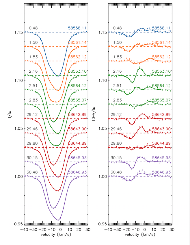
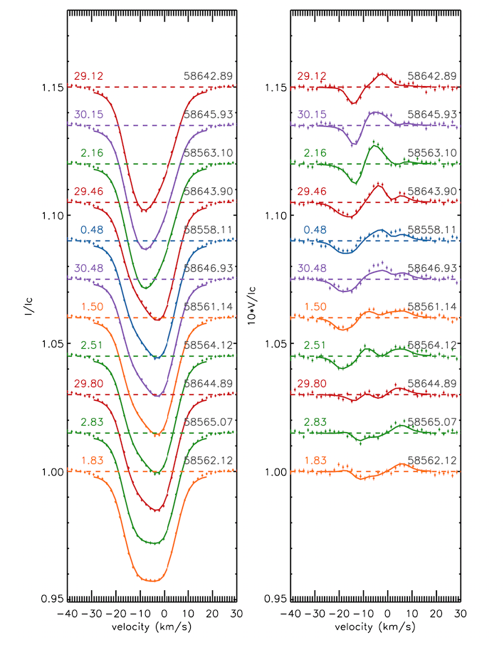
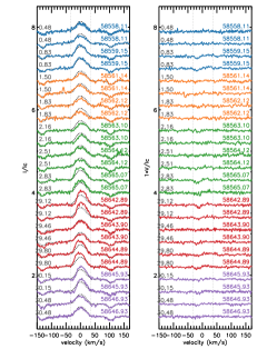
Figure 15: Left: Stokes I and Stokes V LSD profiles ordered as a function of Julian date. Middle: Stokes I and Stokes V LSD profiles ordered as a function of rotational phase. Right: Stokes I and Stokes V profiles of the ${\rm HeI}$ 587.6 nm line’s narrow component ordered as a function of rotational phase. The broad component of the ${\rm HeI}$ line profile has been fitted by a Gaussian and subtracted. The color code corresponds to successive rotational cycles.

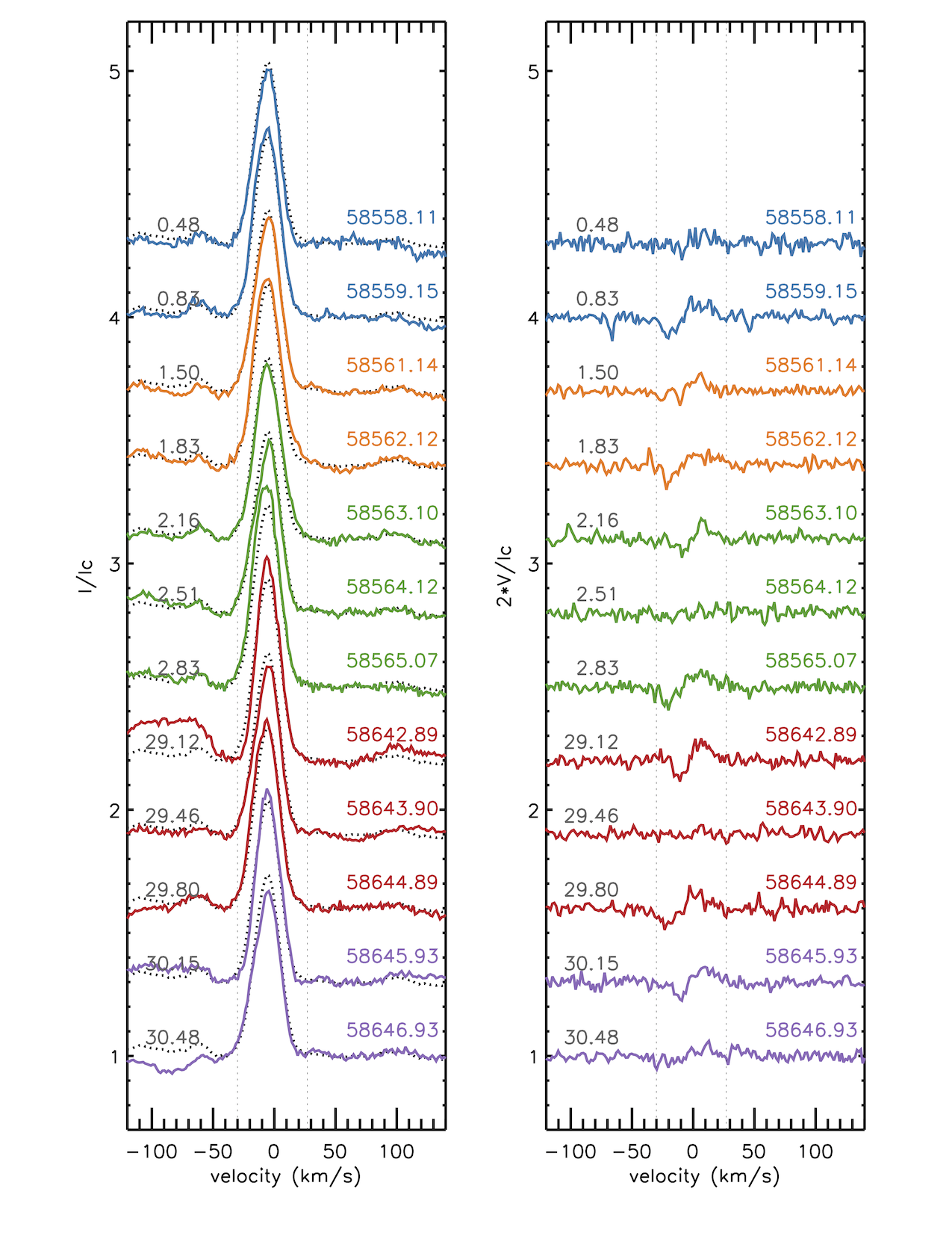
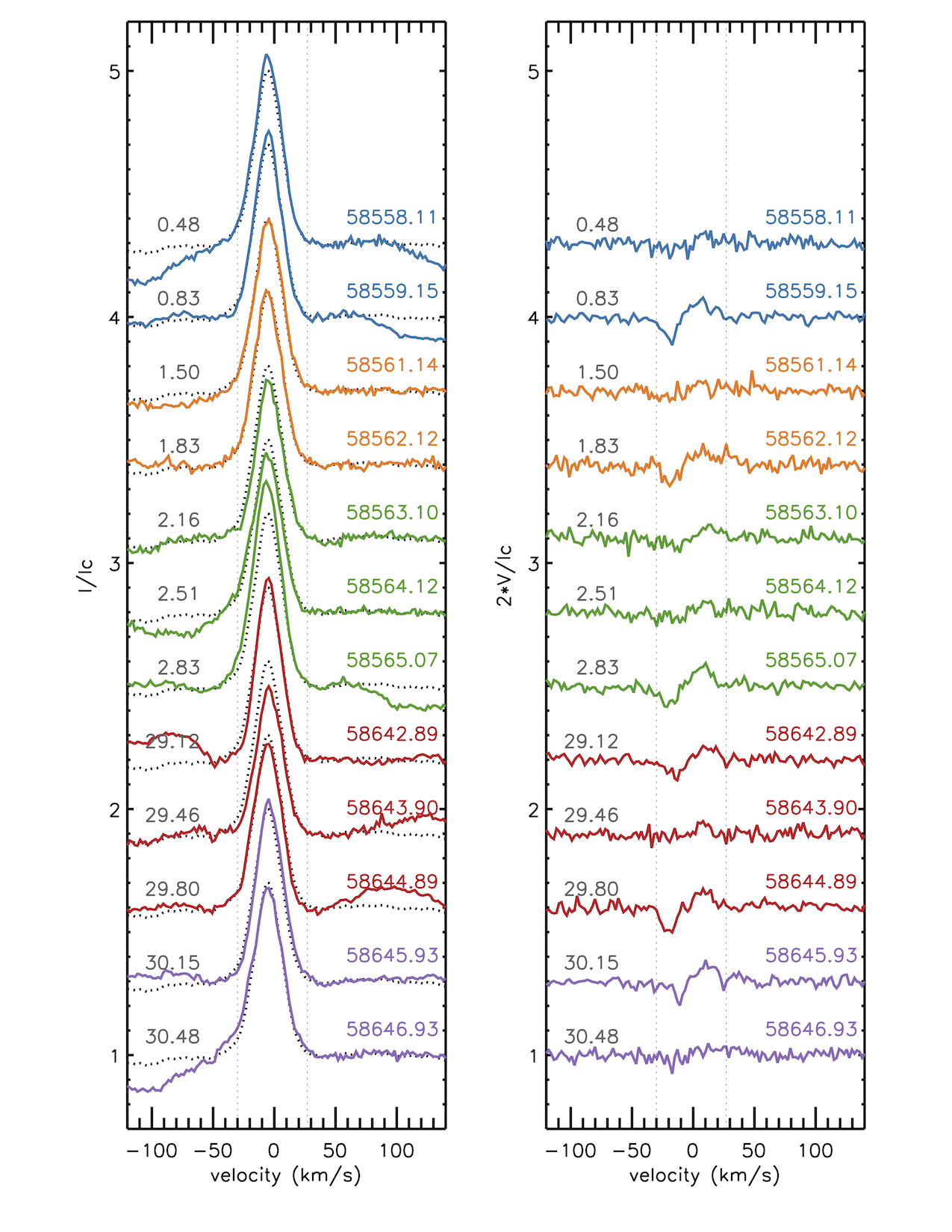
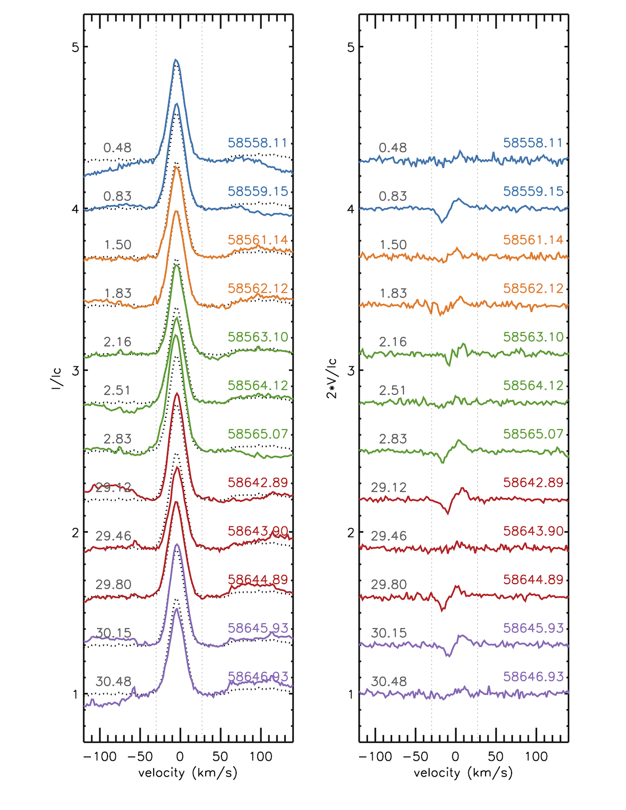
Figure 16: Stokes I (left panels) and V (right panels) profiles ordered as a function of Julian date for the three emission components of the CaII IR triplet: 849 nm (left), 854 nm (middle), 866 nm (right). The phase of the corresponding rotational cycles is indicated on the left of the profiles. The color code corresponds to successive rotational cycles.

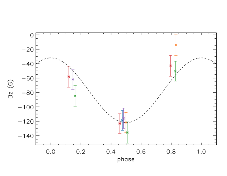
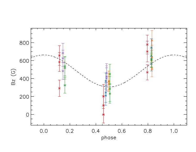
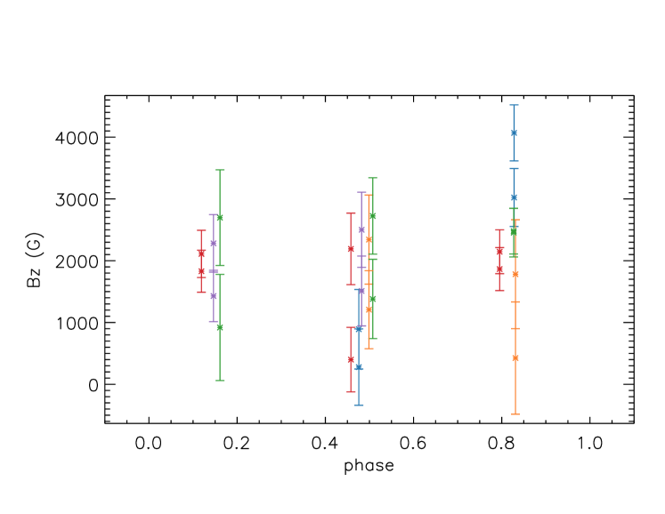
Figure 17: Rotational modulation of the longitudinal component of the large-scale magnetic field, derived from the LSD profiles (top), from the CaII IR triplet (middle), and from the narrow component of the ${\rm HeI}$  587.6 nm lines profile (bottom). The color code corresponds to successive rotational cycles. We emphasize the phase consistency between the March and June datasets, as well as the apparently constant amplitude of the field between the two epochs. In the top panel, the sine curve has been fit with the period and origin of phase of the photometric ephemeris. It shows that the maximum intensity of the photospheric field occurs at phase 0.5, that is, at the time of minimum brightness (see Fig. 3). In the middle panel, the three measurements at each phase are obtained for each line of the CaII IR triplet. In the lower panel, there are two measurements per spectrum, as the ${\rm HeI}$ line appears on successive spectral orders. The three plots are not on the same scale.

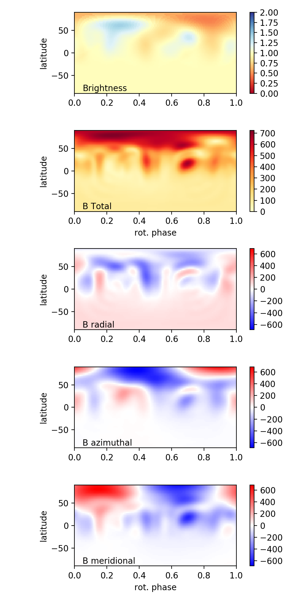
Figure 18: Top: brightness map derived from the variation of the LSD Stokes I profiles. The color code is 1 for the photospheric temperature, increases for hot spots, and decreases for cold ones. Bottom: the large-scale total, radial, longitudinal, and latitudinal surface magnetic field components, as derived from the variations of the LSD Stokes V profiles. The color code indicates the strength of the surface magnetic field in Gauss.

The polarimetric capabilities of CFHT/ESPaDOnS allow us to investigate the large-scale structure of the magnetic field at the surface of the star. Figure 15 shows the least-square deconvolution ((LSD) Donati et al., 1997) Stokes I and Stokes V profiles over the two ESPaDOnS runs, computed using a mean Landé factor of 1.2 and a central wavelength of 500 nm. We did not use the spectrum obtained on JD 8559.15 ($\phi$=0.83) for the ZDI analysis as the LSD profiles show contamination by the morning twilight. A clear and relatively stable magnetic signature is present in all Stokes V profiles. The variation of the longitudinal component of the large scale magnetic field, B_l, derived from the Stokes I and V signatures (Donati et al., 1997; Wade et al., 2000), are shown in Fig. 17. It varies between -14 and -136 Gauss (see Table 5) and appears to be modulated by stellar rotation. Remarkably, the magnetic field intensity does not exhibit significant change between the March and June runs, nor does the phase of its modulation. This suggests a fairly stable magnetic configuration between the two epochs.

A similar analysis has been performed in the CaII near-IR triplet. The three lines of the CaII triplet exhibit consistent magnetic signatures in their Stokes V profiles as shown in Fig. 16. The longitudinal component of the magnetic field projected onto the LoS is still modulated at the stellar rotation period (see Fig. 17) and now reaches a maximum value of 800 G, which is about four times larger than the intensity deduced from the LSD profiles, as is often the case for young accreting stars (e.g., Donati et al., 2019). It is worth mentioning here that the intensity of B_l, as well as its sign, are widely different when using LSD (photospheric) profiles and the CaII IRT (chromospheric) lines. Indeed, these spectral features probe different regions at the stellar surface. The Stokes V signal in the optical ${\rm HeI}$ line was also analyzed, as it provides the most direct estimate of the magnetic field strength at the base of the funnel flow, close to the accretion shock. Unfortunately, the Stokes V profile in the narrow component of the line is weak (see Fig. 15), which translates into large uncertainties in the derivation of the longitudinal field strength. Figure 17 shows the absence of modulation within error bars, with an average field strength of 2$\pm$0.8 kG. The lack of significant modulation may result from the low inclination of the system, where the high latitude accretion shock remains in view during the whole rotational cycle.

We used the Doppler imaging (DI) and Zeeman-Doppler imaging (ZDI) implementation of Folsom et al. (2018) to respectively map the surface brightness and magnetic field of DoAr 44. A full description of the code can be found in Folsom et al. (2018). Briefly, the code uses a time series of Stokes I and V LSD profiles to construct a surface brightness map and the large-scale vector magnetic field. The local line models are calculated using a Voigt profile, with a Gaussian width of 1.2 km s^-1and a Lorentzian width of 1.9 km s^-1. The local line models for Stokes V are calculated from the local I line profile, using the weak-field approximation (Landi Degl’Innocenti & Landolfi, 2004), and the LSD mean Landé factor and central wavelength. The magnetic field is expressed as a combination of spherical harmonics as in Donati et al. (2006). The integration over the surface of the star is done using a linear limb-darkening coefficient of 0.8 (Claret & Bloemen, 2011), adapted to the temperature and gravity of DoAr 44. The fit to the data is performed by both minimizing $\chi^{2}$ and maximizing the entropy, using the maximum entropy fitting routine of Skilling & Bryan (1984). We have adopted the photometric ephemeris defined above, and fixed the inclination of the rotation axis at 35^∘, which is consistent with the inclination of the inner disk seen in interferometry on a scale of 0.14 au (see Paper I).

The resulting brightness and magnetic maps are shown in Fig. 18. One large cool spot is observed on the brightness map, located close to the rotational axis and facing the observer around phase 0.83. Two bright spots are present at lower latitudes, facing the observer around phases 0.30 and 0.70. Due to the low inclination of the system, little is known of the southern hemisphere of the star. We used this brightness map to perform ZDI and reconstruct the magnetic map. We fixed the maximum value of the Legendre polynomial degree $l$ to 15 in the spherical harmonics decomposition. The resulting distribution of the magnetic vectors over the stellar surface is shown in Fig. 18. It indicates a dominant dipolar component, encompassing 75% of the total flux, while only 8% and 4% of the flux is contained in the quadrupolar and octupolar components, respectively. The negative pole of the dipole is facing us at the phase 0.5, which is consistent with the maximum absolute value of the longitudinal field. It is located at the latitude of 70^∘, and thus inclined by 20^∘ onto the rotational axis.

4 Discussion

The variability analysis of the DoAr 44 system is complicated by its nearly integer rotational period of 2.96 d. While we observed the system over several rotational periods, the resulting phase coverage remains limited, with essentially the same three phases being sampled over the observations, at every third of the rotational cycle. This prevents us from having a complete picture of the circumstellar environment of this young stellar object, and also severely limits the longitudinal resolution we have on the stellar surface for image reconstruction. With the data at hand we are nevertheless able to derive the main physical and geometrical properties of the system in the region where the stellar magnetic field interacts with the inner disk.

The combination of the rotational period derived above and the $v\sin i$ we measure suggests that the star is seen at a low inclination of 30$\pm$5$\degr$. In Paper I, we derived a similar inclination of 34$\pm$2$\degr$ for the inner edge of the circumstellar disk from long baseline near-IR interferometry. That the inner system seen at low inclination is further supported by the lack of strong photometric modulation. While we do recover a photometric period of 2.96 d, assigned to the stellar rotational period, the photometric amplitude of $\leq$0.1 mag in the V-band is significantly lower than that of most accreting T Tauri stars (e.g., Grankin et al., 2007). The photospheric radial velocity is modulated over the same 2.96 d period (see Fig. 19), which confirms the presence of a long-lived, large, dark spot at the stellar surface. According to the Doppler image, the high-latitude spot faces the observer at phase 0.83, which yields symmetric LSD profiles (see Fig. 15). Indeed, the photospheric radial velocity lies midway from the extrema of the ${\rm V}_{r}$ curve at this phase, as expected when the spot is on the LoS (see Fig. 19). These concordant results confirm that the 2.96 d period is the rotational period of the star whose surface, seen at a low inclination, is covered by a high-latitude, large, cold spot. In contrast, the photometric minimum appears to occur at phase 0.5, which suggests a more complex distribution of bright and dark spots at the stellar surface drives the photometric modulation.

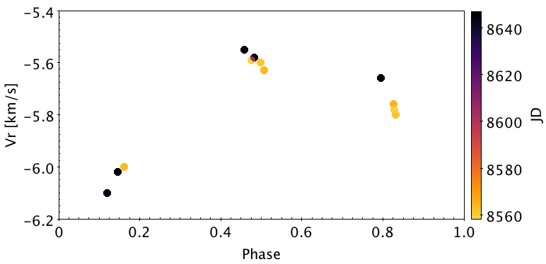
Figure 19: Photospheric radial velocity variations are plotted as a function of rotational phase. The color code reflects the Julian date for the March (bright) and June (dark) ESPaDOnS runs.

In spite of the low inclination, clear modulation signals are also detected in several accretion diagnostics. This is the case of the redshifted wings of emission lines formed in the funnel flow (e.g., ${\rm H}\beta$, ${\rm H}\alpha$, ${\rm Pa}\beta$, ${\rm HeI}$ 1083.3 nm) that smoothly vary along the rotational cycle, even though they do not exhibit inverse P Cygni components, that is, absorptions reaching below the continuum, which are the hallmark of accretion funnel flow passing onto the LoS in high-inclination systems. The radial velocity and the intensity of the narrow component of the ${\rm HeI}$ 587.6 nm line profile are also modulated at the stellar rotational period and indicate a high-latitude hot spot at the stellar surface, presumably the location of the accretion shock close to the magnetic pole. Indeed, the magnetic surface map reconstructed from the ZDI analysis features a dominant dipolar field whose axis is moderately inclined onto the rotational axis, thus producing an accretion shock at high latitudes. These results suggest that the inner disk is truncated at some distance above the stellar surface and that the accretion onto the star proceeds along magnetospheric funnel flows.

If we assume that the disk’s truncation radius lies close to the disk’s corotation radius, we get

$$r_{tr}\simeq r_{co}=(GM_{\star})^{1/3}(P_{rot}/2\pi)^{2/3}=0.043\leavevmode\nobreak\ \rm{au}=9.2\leavevmode\nobreak\ R_{\odot}=4.6\leavevmode\nobreak\ R_{\star},$$

and according to Bessolaz et al. (2008), the truncation radius occurs at

$$r_{tr}/R_{\star}=2\cdot B_{\star}^{4/7}\dot{M}_{acc}^{-2/7}M_{\star}^{-1/7}R_{\star}^{5/7},$$

where the stellar field at the equator B_⋆ is normalized to 140 G, the mass accretion rate $\dot{M}_{\rm acc}$ to 10^-8 ${\rm M}_{\odot}{\rm yr}^{-1}$, the stellar mass ${\rm M}_{\star}$ to 0.8 ${\rm M}_{\odot}$, and the stellar radius ${\rm R}_{\star}$ to 2 ${\rm R}_{\odot}$.

Thus, the condition $r_{tr}\simeq r_{co}$ requires a dipolar magnetic field of the order of 537 G at the equator, which translates into 1.1 kG at the pole. The average value of the longitudinal component of the magnetic field we measure in the narrow component of the ${\rm HeI}$ 587.6 nm line amounts to 2$\pm$0.8 kG. Assuming this is the large scale component that interacts with the disk, we would derive a truncation radius that is about twice the corotation radius. However, the large error bars associated with the field strength and derived from the ${\rm HeI}$ NC component are not inconsistent with the disk being truncated close to the corotation radius. In Paper I, we measured the size of the ${\rm Br}\gamma$ line emitting region, thought to reflect the extent of the magnetospheric cavity, from long baseline near-IR interferometry, and we found it to be less than 0.047 au, that is, 5 ${\rm R}_{\star}$.

All the results summarized above suggest that DoAr 44 was observed during a phase of stable magnetospheric accretion with a magnetic topology that shares some similarities with other young accreting systems that we previously studied, such as V2129~Oph (Alencar et al., 2012). Some of these systems exhibit dipper light curves at times, with deep periodic eclipses of the central object being produced by circumstellar dust: for example, AA~Tau (Bouvier et al., 2003, 2007a) and LkCa~15 (Alencar et al., 2018), as well as periodic redshifted absorptions reaching below the continuum appearing in the wings of emission lines formed in the funnel flow. These specific properties are not shared by DoAr 44 in spite of a qualitatively similar magnetospheric structure. We estimate that the dust sublimation radius lies at a distance of R_sub = 4.7 ${\rm R}_{\star}$= 0.044 au, as derived from Eq.1 of Monnier & Millan-Gabet (2002) for T_sub = 1500 K and Qr=1. Dust might thus to be present at the disk truncation radius, even though the half-flux radius of the inner dusty disk we report in Paper I is of the order of 0.14 au. While a photometric modulation is observed, the light curve is spot dominated, with no evidence for significant dips. Similarly, while the red wing of Balmer line profiles appear modulated at the stellar rotation period, there is no sign of high-velocity redshifted absorptions reaching below the continuum, even at phases where the magnetic pole is facing the observer.

Indeed, dipper characteristics and conspicuous inverse P Cygni profiles are expected to occur primarily in systems seen at a moderate to high inclination (e.g., McGinnis et al., 2015; Sousa et al., 2016; Fonseca et al., 2014). This is clearly not the case in DoAr 44, and the low inclination of this system accounts for the low-amplitude, smooth light curve; the mildly varying red wings of the emission line profiles; and more generally, the global shape of the emission line profiles as suggested by radiative transfer models of magnetospheric accretion onto a misaligned dipole. This clearly highlights the importance of taking into account inclination when investigating the variability of young stellar systems. Systems with otherwise similar properties, notably regarding the magnetospheric accretion process, might exhibit quite different characteristics depending on the viewing angle under which they are seen.

DoAr 44 is a pre-transitional disk system. On the large scale, from mm observations, Andrews et al. (2009, 2011) and van der Marel et al. (2016) reported the existence of a large cavity extending from the central star up to 25-30 au in the circumstellar disk. They showed that cold dust emission arises from an outer, relatively narrow ring (25 to 35 au wide), inclined by 20 to 35° on the LoS. On much smaller scales, the existence of a compact, inner disk close to the star is supported by the near-infrared excess flux measured in the spectral energy distribution of the system (Espaillat et al., 2010) and significant CO emission arising from the inner disk edge (Salyk et al., 2009, 2011). Furthermore, a misalignment between the inner and outer disk was assumed to be responsible for shadows seen in the outer dusty ring (Casassus et al., 2018). In Paper I, we reported the direct detection of the inner disk from long baseline near-IR interferometry. The half-flux radius is 0.14 au, and the compact disk is indeed found to be inclined relative to the outer ring, as predicted by the Casassus et al. (2018) model to account for the outer shadows. The pre-transitional status of DoAr 44’s disk was a strong motivation to include this specific target in our long-term monitoring program of T Tauri stars. The goal here was to investigate whether the highly structured disk, including a large cavity and inner-outer disk misalignment, both possibly betraying ongoing planetary formation, may impact the accretion process on the central star. All the results obtained here suggest that, at the star-disk interaction scale of less than 0.1 au, this pre-transitional disk system is not qualitatively different from other young stellar objects surrounded by smoother protoplanetary disks.

5 Conclusion

We monitored the variability of the young stellar object, DoAr 44, over several rotational periods using several complementary observational techniques to investigate the physics of accretion onto the star in a pre-transitional disk system. The specific geometry of pre-transitional disks, including large cavities and possible inner- or outer-disk misalignment, raises issues regarding the accretion process in these systems. How does accretion proceed from the outer disk to the inner scales through the gap? Is the star-disk interaction process fed in the same way or differently from what is observed in classical T Tauri stars with continuous circumstellar disks? If the pre-transitional nature of disks is the signature of ongoing planet formation in the disk, does this process affect accretion on any scale?

In an attempt to link the outer scales, best studied with mid-IR and radio interferometry, to the inner scales, we focused here on the characterization of the DoAr 44 system at the star-disk interaction level, meaning on a scale extending from the stellar surface up to a few 0.1 au, combining photometric and spectropolarimetric monitoring with long baseline interferometry. The accretion diagnostics studied here and the direct interferometric measurements we reported in Paper I (Bouvier et al., 2020) suggest the existence of an inner magnetospheric cavity extending from a distance of about 4.6 stellar radii (0.043 au) down to the stellar surface. A large-scale, mainly dipolar stellar magnetic field of a few hundred Gauss over the photosphere, but reaching up to 2$\pm$0.8 kG close to the accretion shock, is sufficient to disrupt the inner-disk region at the corotation radius or beyond in this moderately accreting system. The reported line profile variability is consistent with the expected behavior of funnel flows rotating at the stellar period. Yet, due to the low inclination of the inner system, of the order of 30$\degr$, the modulation signatures are not as pronounced as in other, more inclined systems. Importantly, the combination of contemporaneous optical and near-IR high-resolution spectroscopic monitoring provides us with a unique means to investigate diagnostics that simultaneously probe accretion funnel flows and stellar or disk winds.

Overall, over our three-week observation period, DoAr 44 appeared to be in a state of stable magnetospheric accretion, simultaneously driving outflows, in most aspects similar to what we had previously witnessed in other systems we monitored in the same way. This suggests that the physics of accretion from the inner disk to the stellar surface is not significantly altered by the complex large-scale structure of the circumstellar disk specific to pre-transitional systems.

Appendix A Line profile variability

Since the shape of the emisson line profiles has varied between the ESPaDOnS March and June 2019, runs, we present in Fig. 20 their variability over timescales of days, independently for each run.

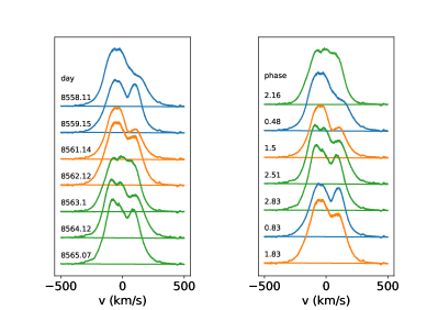
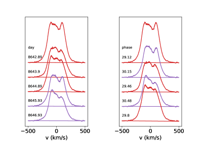
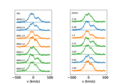
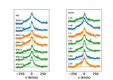
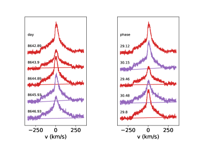
Figure 20: ${\rm H}\alpha$, ${\rm H}\beta$, and ${\rm HeI}$ line profiles from the seven spectra obtained during the ESPaDOnS March run (left panels) and the five spectra obtained during the June run (right panels). In each panel, the profiles are plotted in order of increasing date (left) and phase (right). Each color corresponds to a specific rotational cycle.

The periodogram analysis of line profiles over the two ESPaDOnS runs is inconclusive. We therefore proceed to analyzing the March and June 2019 runs independently. Figures 21 and 22 show the periodogram analysis of the ${\rm H}\alpha$, ${\rm H}\beta$, and ${\rm HeI}$ line profiles for the two epochs, respectively. During the March run, seven spectra were obtained over eight nights, while during the June run, five spectra were obtained over five nights. Moreover, since the stellar period of 2.96 d is close to an integer, the same rotational phase repeats every third night. The short duration of each run combined with the poor phase sampling makes the periodogram analysis fragile. Nevertheless, we find marginal evidence for the rotational frequency of 0.34 d^-1 in the red wing of the ${\rm H}\alpha$ and ${\rm H}\beta$ line profiles around +100 km s^-1 during the March run, and in the narrow central component of the ${\rm HeI}$ line during the June run. While of limited significance, the similar shapes exhibited by the various line profiles at specific rotational phases (see Fig. 20) lends credit to this result. For instance, the Balmer line profiles appear much more symmetric around phases 0.12-0.16 and 0.83-0.93 than around phases 0.46-0.51, where the red wing is consistently depressed. This suggests additional redshifted absorption occurs at phases around 0.5.

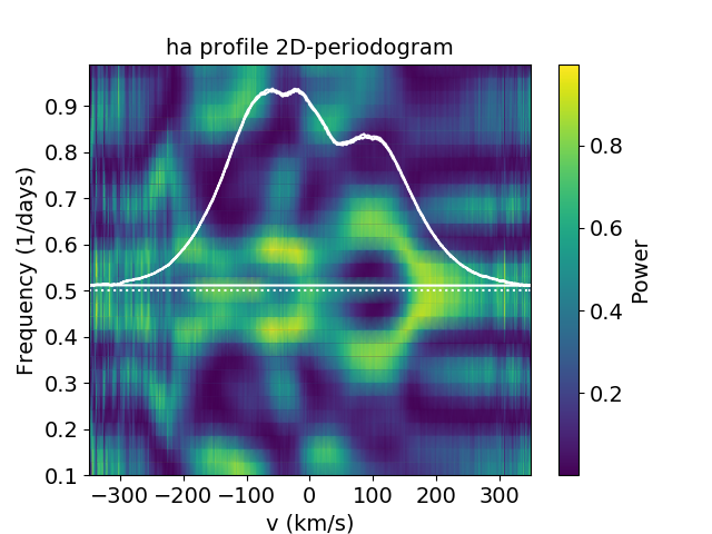
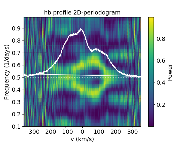
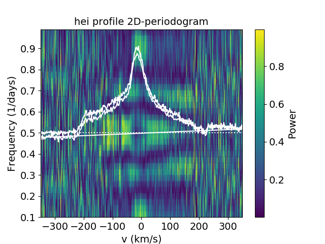
Figure 21: 2D periodogram of ${\rm H}\alpha$, ${\rm H}\beta$, and ${\rm HeI}$ line profiles from the seven spectra obtained during the ESPaDOnS March run. The color code represents the periodogram power, and the superimposed white curve is the average line profile. We note the symmetry of the periodogram around the frequency 0.5 d^-1 due to the 1 d alias resulting from the night-to-night sampling.

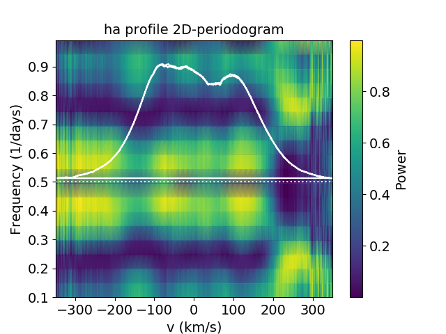
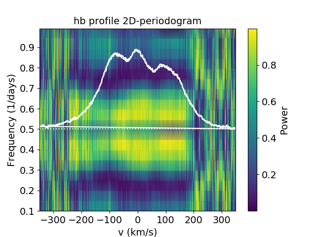
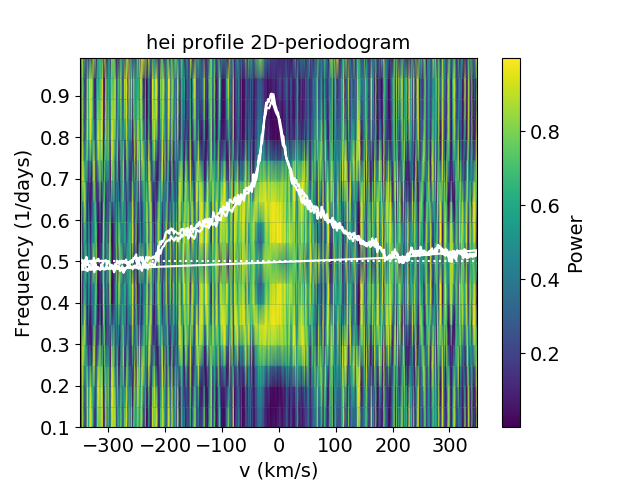
Figure 22: 2D periodogram of ${\rm H}\alpha$, ${\rm H}\beta$, and ${\rm HeI}$ line profiles from the five spectra obtained during the ESPaDOnS June run. The color code represents the periodogram power, and the superimposed white curve is the average line profile. We note the symmetry of the periodogram around the frequency 0.5 d^-1 due to the 1 d alias resulting from the night-to-night sampling.

Appendix B Line profile decomposition

Here, we illustrate examples of line profile decomposition by multiple Gaussian fits for the ${\rm H}\alpha$, ${\rm H}\beta$, ${\rm HeI}$, and CaII emission line profiles observed on JD 8565.07 and JD8644.89. The ${\rm H}\alpha$ and ${\rm H}\beta$ line profiles are well reproduced with a central Gaussian emission peak onto which a blueshifted and a redshifted absorption components are superimposed. The ${\rm HeI}$ line is well fit by the combination of two Gaussian components in emission: a broad one and a narrow one, respectively. This is also the case for the CaII line profile except for two occurrences, on JD 8559.15 and JD 8565.07, where an additional redshifted absorption component is required to reproduce the observed line profile.

Table 8: Gaussian components of optical emission line profiles. The table lists the Julian date, the equivalent width, the peak intensity, radial velocity, and FWHM of the Gaussian fit for each component.

HJD	EW1	EW2	EW3	Int1	${\rm V}_{r}$1	FWHM1	Int2	${\rm V}_{r}$2	FWHM2	Int3	${\rm V}_{r}$3	FWHM3
(-2,450,000)	(Å)	(Å)	(Å)		km s-1	Å		km s-1	Å		km s-1	Å
${\rm H}\alpha$
8558.10852	59.7	-1	-16.4	10	13.1	255.7	-0.8	-39.7	53.1	-4.9	50.3	142.4
8559.15082	50.3	-5.8	-5.5	9	11.9	239.2	-2.7	-7.6	92.8	-3.4	47	67.7
8561.13665	46	-1.1	-12.2	8.7	6.9	226.3	-0.9	-42.8	51.7	-4.8	41.1	107.6
8562.12015	60.9	-8.7	-5.4	10.7	5	242.3	-3.1	-4.2	119.1	-2.7	50.4	84.1
8563.09667	52.2	-5.9	-3.8	9.5	-0.6	235.5	-2.9	-25.1	87.7	-2.3	41.3	69.3
8564.12225	61.2	-2.6	-14	10.5	8.5	249.8	-2	-41.9	55.9	-5.2	39.1	114.9
8565.06818	64	-4.1	-14.5	12.3	4.3	222.1	-2.7	-39.5	63.5	-6.5	29	94.7
8642.8923	86.3	-10.7	-13.8	15	4.9	246.5	-5.4	-34.5	85.1	-6.9	40.2	85.3
8643.89558	60.7	-1.4	-14.6	10.5	14.1	247.9	-1.1	-49.3	54.3	-5	30.6	125.3
8644.89415	69	-2.6	-12.1	11.3	6.5	261.6	-1.9	-41.2	59.2	-4.4	28.4	116.1
8645.93308	60.6	-7.1	-9.9	11.2	16.6	230.3	-3.5	-18.1	86.0	-5.1	49.8	83.4
8646.92779	58.2	-2.1	-16.7	11	12.7	226.5	-1.5	-33.7	57.3	-5.9	33.2	120.8
${\rm H}\beta$
8558.10852	13.9	-0.48	-4.4	3.3	18.9	241.3	-0.5	-41.8	55.2	-2.1	56.4	119.1
8559.15082	7.9	-0.27	-0.9	2	3.6	225.8	-0.31	-41	49.8	-0.8	45	58.3
8561.13665	7.9	-0.13	-1.6	2	1.5	223.3	-0.24	-37.5	31.0	-1.1	48.9	88.1
8562.12015	11.4	-0.33	-1.3	2.9	3.5	227.2	-0.41	-32.9	45.6	-1	41.2	69.6
8563.09667	8.9	-0.55	-0.6	2.4	-5	214.8	-0.59	-34.7	53.8	-0.5	42.5	66.3
8564.12225	15	-0.77	-5.5	3.9	15.5	222.3	-0.78	-39.4	57.3	-2.6	45.8	117.7
8565.06818	10.2	-0.26	-0.8	2.5	-3.9	229.4	-0.34	-32.8	43.5	-0.8	41.7	60.6
8642.8923	18.6	-1.94	-2.3	4.5	4.8	239.0	-1.68	-33.5	67.0	-1.8	39.9	74.0
8643.89558	13.4	-0.45	-4.2	3.3	19.1	231.9	-0.57	-43.7	45.4	-1.8	41.1	128.5
8644.89415	16.3	-1.06	-3	3.9	5.6	238.8	-0.98	-39.6	62.5	-1.5	39.9	113.7
8645.93308	12.9	-0.92	-2.1	3.2	14.5	232.2	-0.9	-34.7	58.8	-1.5	44.2	79.9
8646.92779	13.9	-0.5	-5.2	3.8	18.2	212.4	-0.62	-33.7	47.2	-2.4	39.5	122.2
${\rm HeI}$ 587.6 nm
8558.10852	1.63	0.21		0.31	17.5	248.6	0.22	5.8	47.0
8559.15082	0.81	0.28		0.16	-4.1	238.8	0.31	7.1	43.0
8561.13665	0.99	0.17		0.18	11.1	259.0	0.2	5.6	41.4
8562.12015	1.12	0.19		0.25	-10.4	215.5	0.21	5.9	43.0
8563.09667	0.76	0.17		0.16	-8.5	229.1	0.21	10.9	38.5
8564.12225	1.15	0.23		0.21	5.3	256.6	0.24	5.6	46.8
8565.06818	1.02	0.31		0.21	-10.3	228.0	0.34	7	43.5
8642.8923	1.3	0.32		0.28	-0	221.6	0.4	11.4	38.8
8643.89558	1.1	0.20		0.2	14.1	264.1	0.23	6.1	41.8
8644.89415	1.27	0.33		0.27	0.4	222.8	0.38	4.4	40.9
8645.93308	1.3	0.28		0.27	4.7	228.9	0.35	11.2	38.3
8646.92779	1.12	0.24		0.22	12.7	236.4	0.25	6	46.3
CaII 854.2 nm
8558.10852	6.9	0.62		1.26	19.7	180.5	0.74	0.2	27.3
8559.15082	4.0	0.75	-0.25	0.87	16.7	149.9	0.83	2.1	29.6	-0.1	122.4	84.4
8561.13665	3.3	0.68		0.73	11.7	147.1	0.72	1	31.0
8562.12015	5.1	0.81		1.21	10.3	138.9	0.8	1.4	33.4
8563.09667	4.2	0.62		1	6.6	136.8	0.68	1.8	29.6
8564.12225	5.8	0.69		1.21	14.1	157.0	0.68	-0.2	33.6
8565.06818	4.6	0.92	-0.25	1.01	7.7	149.7	0.94	-0	32.2	-0.1	123.3	83.4
8642.8923	7.4	0.69		1.5	1.6	162.2	0.79	1.7	28.7
8643.89558	4.6	0.60		0.99	13.4	152.0	0.64	1.9	30.8
8644.89415	6.0	0.64		1.22	-6.3	161.2	0.69	-0.5	30.1
8645.93308	5.3	0.77		1.1	13.7	157.5	0.8	2.7	31.3
8646.92779	6.0	0.65		1.28	12.7	151.8	0.65	-0.7	32.9