On the use of Traveling Waves for Pest/Vector elimination using the Sterile Insect Technique

Abstract

The development of sustainable vector/pest control methods is of utmost importance to reduce the risk of vector-borne diseases and pest damages on crops. Among them, the Sterile Insect Technique (SIT) is a very promising one. In this paper, using diffusion operators, we extend a temporal SIT model, developed in a recent paper, into a partially degenerate reaction-diffusion SIT model. Adapting some theoretical results on traveling wave solutions for partially degenerate reaction-diffusion equations, we show the existence of mono-stable and bi-stable traveling-wave solutions for our SIT system. The dynamics of our system is driven by a SIT-threshold number above which the SIT control becomes effective and drives the system to elimination, using massive releases. When the amount of sterile males is lower than the SIT-threshold, the SIT model experiences a strong Allee effect such that a bi-stable traveling wave solution can exist and can also be used to derive an effective long term strategy, mixing massive and small releases. We illustrate some of our theoretical results with numerical simulations, and, also explore numerically spatial-localized SIT control strategies, using massive and small releases. We show that this ”corridor” strategy can be efficient to block an invasion and eventually can be used to push back the front of a vector/pest invasion.

keywords: Sterile insect technique; Vector control; Pest control; Partially degenerate reaction-diffusion system; Allee effect; Traveling wave; Corridor strategy

1 Introduction

Food security and Health security have become of utmost importance around the world because pests and diseases vectors can travel, invade, and settle in new areas causing crop losses and diseases epidemics or pandemics. For instance, according to WHO, 3.9 billons of people are at risk of infection with dengue viruses [7] and modeling estimate indicates that between 284–528 millions of people are infected per year. Dengue is considered as a tropical disease, but as its vectors, like Aedes albopictus [13], are now established in the South of Europe (continuing to spread northward), and also in North-America, the risk of epidemics is real. Similarly, fruit flies, once established, may cause $25$ to $50$ percent losses in food-crop harvests on a very wide range of crops. Among them, the oriental fruit fly, B. dorsalis, is the most damaging one (see [29] for an overview) . Native from Asia, it invaded Africa from 2004, and La Réunion island in 2017. Few individuals have been recorded in Italy in May 2018. Again, being highly invasive, the risk for southern Europa is high.

That is why pest/vector control is absolutely necessary. In the past, most of the control strategies relied on chemical control. Now, we know that this is not sustainable, as chemicals have negative environmental effects, with also the risk of vector/pest resistance appearance in addition to toxic effects on human health, such that most of the chemical cannot be used and are not efficient anymore. Therefore, environmental-friendly vector control and pest management strategies have received widespread attention and have become challenging issues in order to reduce or prevent devastating impact on health, economy, food security, and biodiversity.

One sustainable, environmental-friendly and promising alternative for vector/pest control is the Sterile Insect Technique (SIT). This is an old control technique, proposed in the 30s and 40s by three key researchers in the USSR, Tanzania and the USA and, first, applied in the field in the 50’s [9]. SIT consists to sterilize male pupae using ionizing irradiation and to release a large number of these irradiated males such that they will mate wild females, that will have no viable offspring. Hence, it will result in a progressive decay of the targeted population [3, 9, 14, 15]. For mosquitoes, other sterilization techniques have been developed using either genetics (the Release of Insects carrying a Dominant Lethal, in short RIDL) (see [15, 22] and reference therein), or Cytoplasmic Incompatibility using a bacteria (Wolbachia) [23, 27]. For fruit flies, ionizing radiation has been used so far [9]. However a genetically engineered Medfly (C. capitata) has been developed and tested [5]. Even if, conceptually, the Sterile Insect Technique appears to be very simple, in reality it is not and the process to reach field applications is long and complex [9]. That is why, even if SIT is now used routinely in some places around the world (in Spain or Mexico against the mediterranean fruit flies, for instance), they are still many SIT feasibility projects around the World, including three in France, against Aedes albopictus, vector of Dengue, Chikungunya and Zika in La Réunion, against the fruit fly Ceratitis capitata in Corsica, and the fruit fly Bactrocera dorsalis in La Réunion [4].

We firmly believe that mathematical modeling and computer simulations can be additional and efficient tools within these ongoing programs in order to prevent SIT failures, improve field protocols, and test assumptions before any field investigations, etc.

This work is an extension of [3] where only a mean-field temporal SIT mathematical model was developed and studied aiming to assess the SIT potential as a long term control tool for vector/pest population reduction or elimination, combining massive and small releases. In the present contribution, we take into account vector/pest adult’s dispersal, keeping a certain genericity which allows to apply our spatio-temporal model for several vectors or pests, like mosquitoes or fruit flies.

Very few works exist on SIT taking into account explicitly the spatial component. First because, from the ecological point of view, knowledge are scarce and incomplete. This last point might be strange, but in general it is much more difficult to study the behavior of pest or vector in the field, and, very often, many studies only rely on laboratory or semi-field studies. Also, from the modeling point of view, spatio-temporal models are more difficult to develop and they require more sophisticated tools to be studied. However, some attempts have been made in order to have some insights in SIT systems. In [19], the authors were the first to consider a reaction-diffusion equation to take into account the spreading of a pest in a SIT model. This work was completed in [16], where the release of sterile females was also considered. Tyson et al. [28] used an advection-reaction-diffusion model to study SIT against codling moth in pome fruit orchards. In [20], the authors consider diffusion like in [19], with a time discrete SIT model, to study a barrier strategy. Similarly, Serin Lee et al. [15, 22] studied SIT control with barrier effect using a system of two reaction-diffusion equations for the wild and the sterile populations. In [12], the authors consider discrete cellular automata and show that SIT can fail when oviposition containers distribution is too heterogeneous. A recent work [10] includes impulsive SIT releases. A more complex 2D spatial mosquito model, using a system of coupled ordinary differential equations and advection-reaction-diffusion equations, with applications on SIT, was studied by Dufourd and Dumont [8] highlighting the importance of environmental parameters, like wind, in SIT release strategies. However, no theoretical results were obtained and the results mainly rely on numerical simulations.

The rest of the paper is organized as follows. Section 2 is devoted to recall preliminaries, including theoretical results obtained in [3], that are helpful for our current study. Section 3 deals with the formulation and the study of the spatio-temporal SIT model. We also extend results previously obtained by Fang and Zhao [11] to show existence of monostable and bistable traveling wave solutions for partially degenerate reaction-diffusion equations. In both cases, the wave solution involves the elimination equilibrium or the zero equilibrium and a positive equilibrium. Section 4 deals with numerical simulations in order to support the theoretical results and also go further. In particular, we consider a strategy developed and studied in [3] where massive and small releases were considered to drive a wild population to elimination. Here we extend this strategy using spatially-localized massive releases, within a given (spatial) corridor, coupled with small releases in the pest/vector free area. Finally, in section 5, we summarize the main results and provide future ways to improve or extend this work.

2 Preliminaries

Let us first recall some notations that will be used in this work. Let $\mathcal{C}$ be the set of all bounded and continuous functions from $\mathbb{R}$ to $\mathbb{R}^{n}$. For $u=(u_{1},...,u_{n})^{\prime}$, $v=(v_{1},...,v_{n})^{\prime}\in\mathcal{C}$, we define $u\geq v$ (resp. $u\gg v$) to mean that $u_{i}(x)\geq v_{i}(x)$ (resp. $u_{i}(x)>v_{i}(x)$), $1\leq i\leq n$, $\forall x\in\mathbb{R}$, and $u>v$ to mean that $u\geq v$ but $u\neq v$. Any vector of $\mathbb{R}^{n}$ can be identified as an element in $\mathcal{C}$. For any $r\in\mathbb{R}$, we use boldface r to denote the vector with each component being $r$, i.e., r = $(r,...,r)^{\prime}$. Moreover, for a square matrix $A$, its stability modulus is defined by

$$s(A):=\max\{Re\lambda:\det(\lambda I-A)=0\}.$$

Definition 1.

(Irreducible matrix, [25, page 56])
An $n\times n$ matrix $A=(a_{ij})_{1\leq i,j\leq n}$ is irreducible if for every nonempty, proper subset $I$ of the set $N=\{1,2,...,n\}$, there is an $i\in I$ and $j\in J=N\setminus I$ such that $a_{ij}\neq 0$.

Let $M_{T}(t)$ be the number of sterile insects at time $t$, $1/\mu_{T}$ the average lifespan of sterile insects and $\Lambda$ the number of sterile insects released per unit of time. The dynamics of $M_{T}$ is described by

$$\frac{dM_{T}}{dt}=\Lambda-\mu_{T}M_{T}.$$

Assuming $t$ large enough, we may assume that $M_{T}(t)$ is at its equilibrium value $M_{T}=\Lambda/\mu_{T}$. Following [3], the minimalistic SIT model is defined as follows

$$\left\{\begin{array}[]{lcl}\displaystyle\frac{dA}{dt}&=&\phi F-(\gamma+\mu_{A,1}+\mu_{A,2}A)A,\\ \displaystyle\frac{dM}{dt}&=&(1-r)\gamma A-\mu_{M}M,\\ \displaystyle\frac{dF}{dt}&=&\displaystyle\frac{M}{M+M_{T}}r\gamma A-\mu_{F}F,\\ \end{array}\right.$$ (1)

where parameters and state variables are described in Table 1, page 1. Note also that system (1) is monotone cooperative [25].

Symbol	Description
$A$	Immature stage (gathering eggs, larvae, nymph or pupae stages)
$F$	Fertilized and eggs-laying females
$M$	Males
$\phi$	Number of eggs at each deposit per capita (per day)
$\gamma$	Maturation rate from larvae to adult (per day)
$\mu_{A,1}$	Density independent mortality rate of the aquatic stage (per day)
$\mu_{A,2}$	Density dependent mortality rate of the aquatic stage (per day$\times$ number)
$r$	Sex ratio
$1/\mu_{F}$	Average lifespan of female (in days)
$1/\mu_{M}$	Average lifespan of male (in days)

Table 1: Description of state variables and parameters of model (1)

The basic offspring number related to system (1) is defined as follows

$$\mathcal{R}=\displaystyle\frac{r\gamma\phi}{\mu_{F}(\gamma+\mu_{A,1})}.$$

When $\mathcal{R}>1$, we set

$$Q=\displaystyle\frac{\mu_{A,2}\mu_{M}}{(\gamma+\mu_{A,1})(1-r)\gamma}\quad\mbox{and}\quad M_{T_{1}}=\displaystyle\frac{(\sqrt{\mathcal{R}}-1)^{2}}{Q},$$ (2)

where $M_{T_{1}}$ is the SIT-threshold above which the wild population is driven to elimination. In [3], when $M_{T}=0$, we proved that model (1) admits only the elimination equilibrium, $\bf{0}$ when $\mathcal{R}\leq 1$, and a unique positive equilibrium $E^{*}=(A^{*},M^{*},F^{*})^{\prime}$, the wild equilibrium, in addition to the elimination equilibrium, whenever $\mathcal{R}>1$. Then, assuming $\mathcal{R}>1$, we showed that when $M_{T}\in(0,M_{T_{1}})$ then model (1) has two positive equilibria $E_{1,2}=(A_{1,2},M_{1,2},F_{1,2})^{\prime}$ with $E_{1}<E_{2}$, namely

$$\begin{array}[]{ccl}A_{1,2}&=&\displaystyle\frac{\mu_{M}}{(1-r)\gamma}M_{1,2},\\ F_{1,2}&=&\displaystyle\frac{(\gamma+\mu_{A,1}+\mu_{A,2}A_{1,2})A_{1,2}}{\phi},\\ M_{1}&=&\displaystyle\frac{M_{T}^{*}}{\alpha_{+}},\\ M_{2}&=&\displaystyle\frac{M_{T}^{*}}{\alpha_{-}}.\end{array}$$ (3)

with

$$\begin{array}[]{l}\Delta(M_{T}^{*})=((\sqrt{\mathcal{R}}-1)^{2}-M_{T}^{*}Q)((\sqrt{\mathcal{R}}+1)^{2}-M_{T}^{*}Q),\\ \alpha_{\pm}=\displaystyle\frac{(\mathcal{R}-1-QM_{T}^{*})\pm\sqrt{\Delta(M^{*}_{T})}}{2}.\end{array}$$ (4)

When $M_{T}=M_{T_{1}}$ then the two positive equilibria $E_{1,2}$ collide into a single equilibrium $E_{\dagger}$. The asymptotic behavior of model (1) is summarized in the next theorem.

Theorem 1.

[3]
Assume $\mathcal{R}>1$. System (1) defines a dynamical system on $D=\mathbb{R}^{3}_{+}$ for any $M_{T}\in[0,+\infty)$. Moreover,

1. When $M_{T}>M_{T_{1}}$ then equilibrium 0 is globally asymptotically stable for system (1).

2. When $M_{T}=M_{T_{1}}$ then system (1) has two equilibria 0 and $E_{\dagger}$ with $\textbf{\emph{0}}<E_{\dagger}$. The set $\{x\in\mathbb{R}^{3}:\textbf{\emph{0}}\leq x<E_{\dagger}\}$ is in the basin of attraction of 0 while the set $\{x\in\mathbb{R}^{3}:x\geq E_{\dagger}\}$ is in the basin of attraction of $E_{\dagger}$.

3. When $0<M_{T}<M_{T_{1}}$ then system (1) has three equilibria 0, $E_{1}$ and $E_{2}$ with $\textbf{0}<E_{1}<E_{2}$. The set $\{x\in\mathbb{R}^{3}:\textbf{\emph{0}}\leq x<E_{1}\}$ is in the basin of attraction of 0 while the set $\{x\in\mathbb{R}^{3}:x>E_{1}\}$ is in the basin of attraction of $E_{2}$.

Based on the previous theorem, it is clear that SIT always needs to be maintained. In [3], using the strong Allee effect induced by SIT, we have developed a long term sustainable strategy using, first, massive releases, and then, small releases. Indeed, using massive releases, i.e. $M_{T}>M_{T_{1}}$, we drive the population into the set $\{x\in\mathbb{R}^{3}:\textbf{0}\leq x<E_{1}(M_{T})\}$ for a given (small) value for $M_{T}<<M_{T_{1}}$, in a finite time (see Theorem 4 in [3]). Then, the control goes on with only small releases (see Theorem 5 in [3]). This strategy allows to use a limited number of sterile insects and also to treat large area, step by step.

Now, we take into account the spatial dynamics of the insects. The main objective is to show how a bi-stable traveling wave, generated by the releases of sterile males, can be helpful to control a wild mosquito/pest invasion.

3 A spatio-temporal SIT model

Taking into account adult vectors or pests dispersal through Laplace operators, model (1) becomes the following partially degenerate reaction-diffusion system:

$$\left\{\begin{array}[]{lcl}\displaystyle\frac{\partial A}{\partial t}&=&\phi F-(\gamma+\mu_{A,1}+\mu_{A,2}A)A,\quad(t,x)\in\mathbb{R}_{+}\times\mathbb{R}\\ \displaystyle\frac{\partial M}{\partial t}&=&d_{M}\displaystyle\frac{\partial^{2}M}{\partial x^{2}}+(1-r)\gamma A-\mu_{M}M,\\ \displaystyle\frac{\partial F}{\partial t}&=&d_{F}\displaystyle\frac{\partial^{2}F}{\partial x^{2}}+\displaystyle\frac{M}{M+M_{T}}r\gamma A-\mu_{F}F,\\ \end{array}\right.$$ (5)

where $d_{F}$ and $d_{M}$ denote fertilized females and males diffusion rate, respectively. In addition, system (5) is considered with non-negative and sufficiently smooth initial data. We will now address the question of existence of mono-stable and bistable traveling wave solutions in system (5). Unfortunately, in our case, we cannot apply directly the results from Fang and Zhao [11].

We also need to assume that

$$\mu_{F}<\min\{\mu_{M},\gamma+\mu_{A,1}\}.$$ (6)

Assumption (6) is also consistent with parameter values considered for Aedes spp. in [1, 3, 6, 27].

3.1 Existence and uniqueness of solutions for model (5)

Here, we first address the question of existence and uniqueness of solutions of the reaction-diffusion (RD) system (5) in unbounded domains. For this purpose we will use materials recalled in A.

Let $C_{ub}(\mathbb{R})$ be the Banach space of bounded, uniformly continuous function on $\mathbb{R}$ and,

$$C^{2}_{b}(\mathbb{R})=\{f\in C_{ub}(\mathbb{R}):f^{\prime}\in C_{ub}(\mathbb{R}),\quad f^{\prime\prime}\in C_{ub}(\mathbb{R})\}.$$

$C_{ub}(\mathbb{R})$ and $C^{2}_{b}(\mathbb{R})$ are endowed wit the following (sup) norms

$$\|f\|_{C_{ub}(\mathbb{R})}=\|f\|_{\infty}=\sup\limits_{x\in\mathbb{R}}|f(x)|$$ (7)

and

$$\|g\|_{C_{b}^{2}(\mathbb{R})}=\|g\|_{C_{ub}(\mathbb{R})}+\|g^{\prime}\|_{C_{ub}(\mathbb{R})}+\|g^{\prime\prime}\|_{C_{ub}(\mathbb{R})}.$$ (8)

$C_{b}^{2}(\mathbb{R})$ endowed with the norm $\|\cdot\|_{C_{b}^{2}(\mathbb{R})}$ is a Banach space.

We set $w=(A,M,F)^{\prime}$. System (5) can be written as the abstract Cauchy problem

$$\left\{\begin{array}[]{l}\displaystyle\frac{dw}{dt}+Aw=H(w),\\ w(0)=w_{0}\end{array}\right.$$ (9)

where in the Banach space $B=C_{ub}(\mathbb{R})\times C_{ub}(\mathbb{R})\times C_{ub}(\mathbb{R})$ we have,

$$\left\{\begin{array}[]{l}\eta=diag(0,d_{M},d_{F}),\\ D(A)=C^{2}_{b}(\mathbb{R})\times C^{2}_{b}(\mathbb{R})\times C^{2}_{b}(\mathbb{R}),\\ Aw=-\eta w^{\prime\prime},\\ H:D(A)\rightarrow D(A),\\ H(w)=\left(\phi F-(\gamma+\mu_{A,1}+\mu_{A,2}A)A,(1-r)\gamma A-\mu_{M}M,\displaystyle\frac{M}{M+M_{T}}r\gamma A-\mu_{F}F\right)^{\prime}.\end{array}\right.$$ (10)

For $E\in\{C_{ub}(\mathbb{R}),C^{2}_{b}(\mathbb{R})\}$ and $(a,b,c)\in E\times E\times E$, we define the norm

$$\|(a,b,c)\|_{E\times E\times E}=\|a\|_{E}+\|b\|_{E}+\|c\|_{E}.$$

From [21, Theorem 2.1], we deduce the following Proposition 1.

Proposition 1.

For any $w_{0}\in B$ there is a positive constant $T>0$ depending only on $H$ and $\|w_{0}\|_{B}$, such that system (9) in $[0,T]$, admits a unique local solution $w\in C([0,T],B)$ and

$$w(t)=S(t)w_{0}+\displaystyle\int_{0}^{t}S(t-\tau)H(w(\tau))d\tau,\quad\forall t\in[0,T]$$ (11)

where $\{S(t)\}_{t\geq 0}$ is the Gauss-Weierstrass $C_{0}-$semigroup of contractions defined on the Banach space $B$ (see also (29)-(30), page 29).

In order to prove global (in time) existence of solutions system (9), we use the notion of invariant regions, see e.g. [26, Chapter 14, pages 198-212] and [21].

Lemma 1.

(Invariant rectangles)
Let $k_{1}$ and $k_{2}$ be two real numbers such that $k_{1}>0$ and $k_{2}\geq 1$. The following results hold true.

1. Assume that $\mathcal{R}\leq 1$. The set

   $$\Gamma_{\mathcal{R}\leq 1}=\left\{(A,M,F):(0,0,0)^{\prime}\leq(A,M,F)^{\prime}\leq\left(k_{1},\dfrac{(1-r)\gamma}{\mu_{M}}k_{1},\dfrac{r\gamma}{\mu_{F}}k_{1}\right)^{\prime}\right\}$$

   is positively invariant for system (9).

2. Assume that $\mathcal{R}>1$. The set

   $$\Gamma_{\mathcal{R}>1}=\left\{(A,M,F)^{\prime}:(0,0,0)^{\prime}\leq(A,M,F)^{\prime}\leq\left(k_{2}A^{*},k_{2}M^{*},k_{2}F^{*}\right)^{\prime}\right\}$$

   is positively invariant for system (9).

Proof.

See B. ∎

From the local existence result and the existence of invariant rectangles, we deduce the following global existence result (see e.g. [18, page 307], [21]).

Proposition 2.

For any $w_{0}\in B$, system (9) admits a unique global solution $w\in C([0,+\infty),B)$.

3.2 Existence of traveling waves for model (5)

In compact form, model (5) can be rewritten as follows

$$\frac{\partial U}{\partial t}=D\displaystyle\frac{\partial^{2}U}{\partial x^{2}}+H_{M_{T}}(U),\quad(t,x)\in\mathbb{R}_{+}\times\mathbb{R},$$ (12)

where

$$\begin{array}[]{rcl}U&=&(A,M,F)^{\prime},\\ D&=&diag(0,d_{M},d_{F}),\\ H_{M_{T}}(U)&=&\left(\begin{array}[]{c}\phi F-(\gamma+\mu_{A,1}+\mu_{A,2}A)A\\ (1-r)\gamma A-\mu_{M}M\\ \displaystyle\frac{M}{M+M_{T}}r\gamma A-\mu_{F}F\\ \end{array}\right).\end{array}$$ (13)

To study the traveling wave problem, we consider solution of (19) of the form

$$\begin{array}[]{rcl}A(t,x)&=&A(z),\quad\mbox{ with }z=x+ct\\ M(t,x)&=&M(z),\\ F(t,x)&=&F(z),\end{array}$$ (14)

where $c$ is the wave speed. Therefore, a traveling wave solution of (12) satisfies

$$DU^{\prime\prime}-cU^{\prime}+H_{M_{T}}(U)=0,$$ (15)

where ${}^{\prime}:=\frac{d}{dz}$. We will further assume that

$$U(-\infty)=E_{-\infty},\qquad U(+\infty)=E_{+\infty}$$

where $E_{-\infty}$ and $E_{+\infty}\in\{E^{*};E_{1};E_{2}\}$ are two distinct homogeneous equilibria of (12) with $E_{-\infty}<E_{+\infty}$.

3.2.1 Existence of monostable traveling waves for system (5)

In this section, we first recall some useful results [11]. Consider the $n$-dimensional ($n\geq 2$) reaction-diffusion system

$$\frac{\partial u_{i}}{\partial t}=d_{i}\displaystyle\frac{\partial^{2}u_{i}}{\partial x^{2}}+f_{i}(u_{1},...,u_{n}),\quad(t,x)\in\mathbb{R}_{+}\times\mathbb{R},\quad 1\leq i\leq n,$$ (16)

where, some, but not all, diffusion coefficients $d_{i}$ are zero, and the others are positive. Let us set $D:=diag(d_{1},...,d_{n})$.

Recall that for a square matrix $Y$, the stability modulus is defined as follows:

$$s(Y)=\max\{\text{Re}\sigma/\det(\sigma I-Y)=0\}.$$

To prove the existence of monostable traveling wave solutions for system (16), Fang and Zhao [11] consider the following assumptions:

(H) Assume that $f=(f_{1},...,f_{n})^{\prime}:\mathbb{R}^{n}\rightarrow\mathbb{R}^{n}$ satisfies the following assumptions:

1. $f$ is continuous with $f(\textbf{0})=f(\textbf{1})=\textbf{0}$ and there is no $\nu$ other than 0 and 1 such that $f(\nu)=$ 0 with 0 $\leq\nu\leq$ 1.

2. System (16) is cooperative.

3. $f(u)$ is piecewise continuously differentiable in $u$ for 0 $\leq\nu\leq$ 1 and differentiable at 0, and the matrix $f^{\prime}(\textbf{0})$ is irreducible, with $s(f^{\prime}(\textbf{0}))>0$.

For practical applications, $f^{\prime}(\bf{0})$ irreducible, in item (H)₃, is quite restrictive. However in the proof of their results, Fang and Zhao [11] needed only a consequence of this irreducibility property, deduced also from the Perron-Frobenius Theorem (see [25, chapter 4, section 3]). So we can weaken this irreducibility assumption and consider its consequence, such that (H) now becomes:

(H’) Assume that $f=(f_{1},...,f_{n})^{\prime}:\mathbb{R}^{n}\rightarrow\mathbb{R}^{n}$ satisfies assumptions (H)₁, (H)₂, and

1. $f(u)$ is piecewise continuously differentiable in $u$ for 0 $\leq\nu\leq$ 1 and differentiable at 0, and for $\mu>0$ the matrix $A(\mu):=\mu^{2}D+f^{\prime}(\emph{{0}})$ is such that $\lambda(\mu)=s(A(\mu))>0$ is a simple eigenvalue of $A(\mu)$ with a strongly positive eigenvector $v(\mu)=(v_{1}(\mu),...,v_{n}(\mu))$ with $\|v(\mu)\|=1$.

For $\mu>0$, we define the function $\Phi(\mu):=\lambda(\mu)/\mu>0$ and $\overline{c}:=\inf\limits_{\mu>0}\Phi(\mu)>0.$ Suppose also that $\overline{\mu}\in(0,+\infty)$ is the value of $\mu$ at which $\Phi(\mu)$ attains its infimum. The following result is valid

Lemma 2.

Assume that (H’) holds. Let $\phi\in\{u\in\mathcal{C}:\textbf{0}\leq u\leq\textbf{1}\}$ and $u(t,x;\phi)$ be the unique solution of (the integral form of) (16) through $\phi$. Then there exists a real number $c^{*}\geq\overline{c}>0$ such that the following statements are valid:

• If $\phi$ has compact support, then $\lim\limits_{t\rightarrow+\infty,|x|\geq ct}u(t,x;\phi)=\textbf{0}$, $\forall c>c^{*}$.

• For any $c\in(0,c^{*})$ and $r>0$, there is a positive number $R_{r}$ such that for any $\phi\in\{u\in\mathcal{C}:\textbf{0}\leq u\leq\textbf{1}\}$ with $\phi\geq\textbf{r}$ on an interval of length $2R_{r}$ , there holds $\lim\limits_{t\rightarrow+\infty,|x|\leq ct}u(t,x;\phi)=\textbf{1}$.

• If, in addition, $f(\min\{\rho v(\overline{\mu}),\textbf{\emph{1}}\})\leq\rho f^{\prime}(\textbf{\emph{0}})v(\overline{\mu})$, $\forall\rho>0$, then $c^{*}=\overline{c}$.

Proof.

The results follow from [11, Lemma 2.3] by considering assumption (H’) instead of (H). ∎

We observe that in Lemma 2, assumption stated in item $(iii)$ implies that $f(u)$ is dominated by its linearization at 0 in the direction of $v(\overline{\mu})$ and this ensures the so-called linear determinacy property ([30], [17] and references therein).

Fang and Zhao [11] further consider the following assumption.
(K) Assume that $f=(f_{1},...,f_{n})^{\prime}:\mathbb{R}^{n}\rightarrow\mathbb{R}^{n}$ is such that:

1. $f$ is continuous with $f(\textbf{0})=f(\textbf{1})=\textbf{0}$ and there is no $\nu$ other than 0 and 1 such that $f(\nu)=$ 0 with 0 $\leq\nu\leq$ 1.

2. System (16) is cooperative.

3. $f(u)$ is piecewise continuously differentiable in $u$ for 0 $\leq\nu\leq$ 1 and differentiable at 0, and the matrix $f^{\prime}(\textbf{0})$ is irreducible with $s(f^{\prime}(\textbf{0}))>0$.

4. There exist $a>0$, $\sigma>1$ and $r>0$ such that $f(u)\geq f^{\prime}(\textbf{0})u-a\|u\|^{\sigma}$1 for all 0$\leq u\leq\textbf{\emph{r}}$.

5. For any $\rho>0$, $f(\min\{\rho v(\mu),\textbf{1}\})\leq\rho f^{\prime}(\textbf{0})v(\mu)$, $\forall\mu\in(0,\overline{\mu}]$, where $\overline{\mu}$ is the value of $\mu$ at which $\Phi(\mu)$ attains its infimum.

As previously, we weaken the third statement of (K) and it now reads as:

(K’) Assume that $f=(f_{1},...,f_{n}):\mathbb{R}^{n}\rightarrow\mathbb{R}^{n}$ satisfies assumptions (K)₁, (K)₂, (K)₄, (K)₅, and

1. $f(u)$ is piecewise continuously differentiable in $u$ for 0 $\leq\nu\leq$ 1 and differentiable at 0, and for $\mu>0$ the matrix $A(\mu):=\mu^{2}D+f^{\prime}(\textbf{0})$ is such that $\lambda(\mu)=s(A(\mu))>0$ is a simple eigenvalue of $A(\mu)$ with a strongly positive eigenvector $v(\mu)=(v_{1}(\mu),...,v_{n}(\mu))$ with $\|v(\mu)\|=1$.

Then, the following results hold

Theorem 2.

Assume that (K’) holds and let $c^{*}$ be defined as in Lemma 2. Then for each $c\geq c^{*}$, system (16) has a nondecreasing wavefront $U(x+ct)$ connecting 0 and 1; while for any $c\in(0,c^{*})$, there is no wavefront $U(x+ct)$ connecting 0 and 1.

Proof.

The results follow from [11, Theorem 3.1] by considering (K’) instead of (K). ∎

Now we are in position to study the existence of monostable traveling wave solutions for model (12) when no SIT control occurs, i.e. $M_{T}=0$. System (12) becomes

$$H_{M_{T}}(U)=H_{0}(U)=\left(\begin{array}[]{c}\phi F-(\gamma+\mu_{A,1}+\mu_{A,2}A)A\\ (1-r)\gamma A-\mu_{M}M\\ r\gamma A-\mu_{F}F\\ \end{array}\right).$$ (17)

From section 2, we deduce that $H_{0}(U)=\textbf{0}$ has two solutions $E_{0}=\textbf{0}$ and $E^{*}=(A^{*},M^{*},F^{*})^{T}$, with $s(H^{\prime}_{0}(E_{0}))>0$ and $s(H^{\prime}_{0}(E^{*}))<0$ where $H^{\prime}_{0}(U)$ denotes the Jacobian matrix of $H_{0}$ at $U$. To follow the ideas developed by Fang and Zhao [11] and for sake of clarity, we first normalize system (12) -(17). For this purpose, we set

$$a=A/A^{*},\quad m=M/M^{*},\quad f=F/F^{*}.$$

Thus, system (12) -(17) becomes

$$\frac{\partial u}{\partial t}=D\displaystyle\frac{\partial^{2}u}{\partial x^{2}}+h_{0}(u),\quad(t,x)\in\mathbb{R}_{+}\times\mathbb{R},$$ (18)

where

$$\begin{array}[]{lcl}u&=&(a,m,f)^{T},\\ D&=&diag(0,d_{M},d_{F}),\\ h_{0}(u)&=&\left(\begin{array}[]{c}(\gamma+\mu_{A,1})(\mathcal{R}f-a-(\mathcal{R}-1)a^{2})\\ \mu_{M}(a-m)\\ \mu_{F}(a-f)\\ \end{array}\right).\end{array}$$ (19)

Thus, obviously, system (18) is cooperative and admits only two homogeneous equilibria, $e_{0}=\bf{0}$ and $e^{*}=\bf{1}$, such that (H’)₁ and (H’)₂ are verified. Similarly, since the right hand-side is a two-order polynomial, it is easy to show that (K’)₄ holds too, i.e. $h_{0}(u)\geq h^{\prime}_{0}(\textbf{0})u-(\mathcal{R}-1)(\mu_{A,1}+\gamma)\|u\|^{2}\textbf{1}$, for all $\textbf{0}\leq u\leq\textbf{1}$.

Now, we need to check (K’)₃ and (K’)₅. For $\mu>0$ let us define

$$\omega(\mu)=\mu^{2}D+h_{0}^{\prime}(\textbf{0})=\left(\begin{array}[]{ccc}-(\mu_{A,1}+\gamma)&0&\mathcal{R}(\mu_{A,1}+\gamma)\\ \mu_{M}&-\mu_{M}+\mu^{2}d_{M}&0\\ \mu_{F}&0&-\mu_{F}+\mu^{2}d_{F}\\ \end{array}\right).$$ (20)

The eigenvalues of $\omega(\mu)$ are $\sigma_{3}=-\mu_{M}+\mu^{2}d_{M}$ and the solutions of the second order equation

$$\sigma^{2}+\sigma(-\mu^{2}d_{F}+\mu_{F}+\mu_{A,1}+\gamma)+\mu_{F}(\mu_{A,1}+\gamma)(1-\mathcal{R})-(\mu_{A,1}+\gamma)\mu^{2}d_{F}=0.$$ (21)

Since $\Delta=(-\mu^{2}d_{F}+\mu_{F}+\mu_{A,1}+\gamma)^{2}+4\mu_{F}(\mu_{A,1}+\gamma)(\mathcal{R}-1)+4(\mu_{A,1}+\gamma)\mu^{2}d_{F}>0$, we deduce that

$$\sigma_{1}=\displaystyle\frac{-(-\mu^{2}d_{F}+\mu_{F}+\mu_{A,1}+\gamma)-\sqrt{\Delta}}{2}<0,$$

$$\sigma_{2}=\displaystyle\frac{-(-\mu^{2}d_{F}+\mu_{F}+\mu_{A,1}+\gamma)+\sqrt{\Delta}}{2}>0.$$

Obviously, we have $\sigma_{2}>\sigma_{1}$. Since $\mu_{F}<\mu_{M}$ and $d_{F}\geq d_{M}$, we have

$$\sigma_{2}-\sigma_{3}=\frac{\sqrt{\Delta}-(\mu_{A,1}+\gamma+\mu_{F}-\mu^{2}d_{F})}{2}+\left(\mu_{M}-\mu^{2}d_{M}\right)\geq\frac{\sqrt{\Delta}-(\mu_{A,1}+\gamma-(\mu_{F}-\mu^{2}d_{F}))}{2},$$

that is

$$\begin{array}[]{lcl}\sigma_{2}-\sigma_{3}\geq\dfrac{\Delta-(\mu_{A,1}+\gamma-(\mu_{F}-\mu^{2}d_{F}))^{2}}{2(\sqrt{\Delta}+(\mu_{A,1}+\gamma+\mu_{F}-\mu^{2}d_{F})}&=&\dfrac{4\mu_{F}(\mu_{A,1}+\gamma)\mathcal{R}}{2(\sqrt{\Delta}+(\mu_{A,1}+\gamma+\mu_{F}-\mu^{2}d_{F})}\\ &=&{\color[rgb]{0,0,0}\dfrac{\mu_{F}(\mu_{A,1}+\gamma)\mathcal{R}}{-\sigma_{1}}}>0,\end{array}$$

such that $\sigma_{2}>\max(\sigma_{1},\sigma_{3})$.

Now we compute an eigenvector $v_{0}=(x,y,z)^{\prime}$ of $\omega(\mu)$ associated to $\sigma_{2}$. We need to solve the algebraic equations

$$\left\{\begin{array}[]{rcc}-(\mu_{A,1}+\gamma)x+R(\mu_{A,1}+\gamma)z&=&\sigma_{2}x,\\ \mu_{M}x-\mu_{M}y+\mu^{2}d_{M}y&=&\sigma_{2}y,\\ \mu_{F}x+(\mu^{2}d_{F}-\mu_{F})z&=&\sigma_{2}z.\end{array}\right.$$

From the last two equations, since $\sigma_{2}>\mu^{2}d_{F}-\mu_{F}$ and $\sigma_{2}>\sigma_{3}$, we obtain

$$\left\{\begin{array}[]{ccl}y&=&\dfrac{\mu_{M}}{\sigma_{2}+\mu_{M}-\mu^{2}d_{M}}x=\dfrac{\mu_{M}}{\sigma_{2}-\sigma_{3}}x,\\ z&=&\displaystyle\frac{\mu_{F}}{\sigma_{2}+\mu_{F}-\mu^{2}d_{F}}x.\end{array}\right.$$

Substituting into the first equation leads to

$$\begin{array}[]{cl}&-(\mu_{A,1}+\gamma)x+\mathcal{R}(\gamma+\mu)\displaystyle\frac{\mu_{F}}{\sigma_{2}+\mu_{F}-\mu^{2}d_{F}}x=\sigma_{2}x,\\ \Leftrightarrow&(-(\mu_{A,1}+\gamma)(\sigma_{2}+\mu_{F}-\mu^{2}d_{F}+\mathcal{R}(\mu_{A,1}+\gamma)\mu_{F}))x=(\sigma_{2}+\mu_{F}-\mu^{2}d_{F})\sigma_{2}x\\ \Leftrightarrow&(\sigma_{2}^{2}+\sigma_{2}(-\mu^{2}d_{F}+\mu_{F}+\mu_{A,1}+\gamma)+\mu_{F}(\mu_{A,1}+\gamma)(1-\mathcal{R})-(\mu_{A,1}+\gamma)\mu^{2}d_{F})x=0.\end{array}$$

Since $\sigma_{2}$ is a positive root of (21), we deduce that $x\in\mathbb{R}^{*}$. Therefore, setting $x=1$, we deduce

$$v_{0}=\left(1,\displaystyle\frac{\mu_{M}}{\sigma_{2}+\mu_{M}-\mu^{2}d_{M}},\displaystyle\frac{\mu_{F}}{\sigma_{2}+\mu_{F}-\mu^{2}d_{F}}\right)^{\prime}>\textbf{0}.$$

Then, we set

$$v(\mu)=\displaystyle\frac{1}{\|v_{0}\|}v_{0}$$ (22)

such that $\|v(\mu)\|=1$. Thus (K’)₃ holds.

Let us consider, for $\mu>0$,

$$\Phi(\mu)=\sigma_{2}(\mu)/\mu>0.$$

Since $\Phi(\mu)>\mu d_{F}-\displaystyle\frac{\mu_{F}}{\mu}$, it implies that $\lim\limits_{\mu\rightarrow+\infty}\Phi(\mu)=+\infty$. Similarly, since $\lim\limits_{\mu\rightarrow 0}\sigma_{2}(\mu)>0$, we also deduce that $\lim\limits_{\mu\rightarrow 0^{+}}\Phi(\mu)=+\infty$. In addition,

$$\Phi^{\prime}(\mu)=0\Leftrightarrow\psi(\mu):=\mu\sigma^{\prime}_{2}(\mu)-\sigma_{2}(\mu)=0.$$

Direct computations lead that

$$\psi(\mu)=\displaystyle\frac{\mu^{2}d_{F}+\mu_{F}+\mu_{A,1}+\gamma}{2}+\displaystyle\frac{\mu^{2}d_{F}(\mu^{2}d_{F}-\mu_{F}+\mu_{A,1}+\gamma)}{\sqrt{\Delta}}-\displaystyle\frac{\Delta}{2\sqrt{\Delta}}.$$

Thus, $\psi(\mu)=0$ is equivalent to

$$(\mu^{2}d_{F}+\mu_{F}+\mu_{A,1}+\gamma)^{2}\Delta-(2\mu^{2}d_{F}(\mu^{2}d_{F}-\mu_{F}+\mu_{A,1}+\gamma)-\Delta)^{2}=0.$$

Let us set:

$$\begin{array}[]{cl}x&=\mu^{2}d_{F},\\ a_{1}&=\mu_{A,1}+\gamma,\\ a_{2}&=\mu_{F}+a_{1},\\ a_{3}&=\mu_{F}(\mathcal{R}-1),\end{array}$$

such that $\Delta=(a_{2}-x)^{2}+4a_{1}(a_{3}+x)$. Then, solving $\psi(\mu)=0$ is equivalent to

$$(x+a_{2})^{2}((a_{2}-x)^{2}+4a_{1}(x+a_{3}))-(2x(x-a_{2}+2a_{1})-((a_{2}-x)^{2}+4a_{1}(x+a_{3})))^{2}=0,$$

$$((x+a_{2})(a_{2}-x))^{2}-(2x(x+2a_{1})-a_{2}^{2}-x^{2}+4a_{1}(x+a_{3})))^{2}+4a_{1}(x+a_{2})^{2}(x+a_{3})=0,$$

$$((x+a_{2})(a_{2}-x))^{2}-(x^{2}-a_{2}^{2}-4a_{1}a_{3}))^{2}+4a_{1}(x+a_{2})^{2}(x+a_{3})=0,$$

$$(a_{2}^{2}-x^{2})^{2}-(x^{2}-a_{2}^{2}-4a_{1}a_{3}))^{2}+4a_{1}(x+a_{2})^{2}(x+a_{3})=0,$$

$$-4a_{1}a_{3}(2a_{2}^{2}-2x^{2}+4a_{1}a_{3})+4a_{1}(x+a_{2})^{2}(x+a_{3})=0.$$

Simplifying by $4a_{1}$ and expanding the previous terms lead to

$$x^{3}+(3a_{3}+2a_{2})x^{2}+(2a_{2}a_{3}+a_{2}^{2})x-(a_{3}a_{2}^{2}+4a_{1}a_{3}^{2})=0.$$ (23)

All coefficients are positive except the last one, such that $\psi(\mu)=0$ has a unique positive root which ensures that $\Phi^{\prime}$ changes sign once on $(0,+\infty)$. Thus, taking into account the computations on the limits of $\Phi$ and the continuity of $\Phi$, we deduce that there exists a unique $\overline{\mu}>0$ such that $\Phi(\overline{\mu})=\inf\limits_{\mu>0}\Phi(\mu)>0$, the so-called minimal speed

$$\overline{c}:=\dfrac{\sigma_{2}(\overline{\mu})}{\overline{\mu}}.$$ (24)

Let $\mu\in(0,\bar{\mu}]$ and $\rho>0$.

$$\begin{array}[]{cll}h_{0}(\rho v(\mu))&=&\left(\begin{array}[]{c}(\mu_{A,1}+\gamma)(\mathcal{R}\rho v_{3}-\rho v_{1}-(\mathcal{R}-1)(\rho v_{1})^{2})\\ \rho\mu_{M}(v_{1}-v_{2})\\ \rho\mu_{F}(v_{1}-v_{3})\\ \end{array}\right)\\ &\leq&\rho\left(\begin{array}[]{c}(\mu_{A,1}+\gamma)(\mathcal{R}v_{3}-v_{1})\\ \mu_{M}(v_{1}-v_{2})\\ \mu_{F}(v_{1}-v_{3})\\ \end{array}\right)\\ &=&\rho h_{0}^{\prime}(\textbf{0})v(\mu)\end{array}$$ (25)

where $v(\mu)=(v_{1}(\mu),v_{2}(\mu),v_{3}(\mu))^{\prime}$ is defined in (22). Therefore, since (H’) and (K’) hold true, we can apply Lemma 2, page 2, and Theorem 2, page 2 to system (18), to deduce that the spreading speed $c^{*}$ coincides with the minimal wave speed, $\overline{c}$, defined in (24), and the following result for system (5)

Theorem 3.

For each $c\geq c^{*}=\overline{c}$, system (5) has a nondecreasing wavefront $U(x+ct)$ connecting $E_{0}$ and $E^{*}$; while for any $c\in(0,c^{*})$, there is no wavefront $U(x+ct)$ connecting $E_{0}$ and $E^{*}$.

3.2.2 Existence of bistable traveling waves for system (5)

To show existence of bistable traveling wave solutions of system (16), Fang and Zhao [11] considered the following assumptions:
(L) Assume that $f=(f_{1},...,f_{n})^{\prime}\in\mathcal{C}^{1}(\mathbb{R}^{n},\mathbb{R}^{n})$ satisfies the following assumptions:

1. $f(\textbf{0})=f(\textbf{1})=f(\alpha)=\textbf{0}$ with 0$\ll\alpha\ll$1. There is no $\nu$ other than 0, 1 and $\alpha$ such that $f(\nu)=$ 0 with 0 $\leq\nu\leq$ 1.

2. System (16) is cooperative.

3. $u\equiv\textbf{0}$ and $u\equiv\textbf{1}$ are stable, and $u\equiv\alpha$ is unstable, that is,

   $$\lambda_{0}:=s(f^{\prime}(\textbf{0}))<0,\quad\lambda_{1}:=s(f^{\prime}(\textbf{1}))<0,\quad\lambda_{\alpha}:=s(f^{\prime}(\alpha))>0.$$

4. $f^{\prime}(\textbf{0})$, $f^{\prime}(\textbf{1})$ and $f^{\prime}(\alpha)$ are irreducible.

Then, they showed the following result

Theorem 4.

( [11, Theorem 4.1] - bistable TW)
Assume that (L) holds. Then system (16) admits a monotone wavefront $(U,c)$ with $U(-\infty)=\textbf{0}$ and $U(+\infty)=\textbf{1}.$

Practically, in assumption (L), the last item concerning the irreducibility of matrices $f^{\prime}(\textbf{0})$, $f^{\prime}(\textbf{1})$ and $f^{\prime}(\alpha)$, is quite restrictive for application. We found that we can weaker this assumption as follows:

(L’): assume that $f\in\mathcal{C}^{1}(\mathbb{R}^{n},\mathbb{R}^{n})$ satisfies assumptions (L)₁, (L)₂, (L)₃ and

1. There exists an eigenvector $e_{0}\gg\textbf{0}$ with $||e_{0}||_{\mathbb{R}^{n}}=1$ corresponding to $\lambda_{0}$, $f^{\prime}(\textbf{1})$ and $f^{\prime}(\alpha)$ are irreducible.

or

(L”): assume that $f\in\mathcal{C}^{1}(\mathbb{R}^{n},\mathbb{R}^{n})$ satisfies assumptions (L)₁, (L)₂, (L)₃ and

1. There exist eigenvectors $e_{0}\gg\textbf{0}$ and $e_{1}\gg\textbf{0}$ with $||e_{0}||_{\mathbb{R}^{n}}=||e_{1}||_{\mathbb{R}^{n}}=1$ corresponding to $\lambda_{0}$ and $\lambda_{1}$ respectively, and $f^{\prime}(\alpha)$ is irreducible.

We obtain the following result

Theorem 5.

Assume (L’) or (L”) holds. Then system (16) admits a monotone wavefront $(U,c)$ with $U(-\infty)=\textbf{0}$ and $U(+\infty)=\textbf{1}.$

Proof.

The proof is exactly the same as the proof of Theorem 4.1 in Fang and Zhao [11]. ∎

Coming back to the SIT PDE model (12), with $0<M_{T}<M_{T_{1}}$, the Jacobian matrix at the extinction equilibrium $E_{0}=\textbf{0}$ is

$$H^{\prime}(E_{0})=\left(\begin{array}[]{ccc}-(\gamma+\mu_{A,1})&0&\phi\\ (1-r)\gamma&-\mu_{M}&0\\ 0&0&-\mu_{F}\\ \end{array}\right).$$

From (6), we infer

$$\lambda_{0}=s(H^{\prime}(E_{0}))=\max\{-(\gamma+\mu_{A,1}),-\mu_{M},-\mu_{F}\}=-\mu_{F}.$$

Let $u=(x,y,z)^{\prime}$ be an eigenvector of $H^{\prime}(E_{0})$ that correspond to $\lambda_{0}$, that is

$$\left\{\begin{array}[]{rcl}-(\gamma+\mu_{A,1})x+\phi z&=&\lambda_{0}x,\\ (1-r)\gamma x-\mu_{M}y&=&\lambda_{0}y,\\ z&\in&\mathbb{R}.\end{array}\right.$$

From assumption (6), that $x=\displaystyle\frac{\phi}{\gamma+\mu_{A,1}-\mu_{F}}z$ and $y=\displaystyle\frac{\phi(1-r)\gamma}{(\gamma+\mu_{A,1}-\mu_{F})(\mu_{M}-\mu_{F})}z$. Therefore one can choose

$$u=(x,y,z)^{\prime}=\left(\displaystyle\frac{\phi}{\gamma+\mu_{A,1}-\mu_{F}},\displaystyle\frac{\phi(1-r)\gamma}{(\gamma+\mu_{A,1}-\mu_{F})(\mu_{M}-\mu_{F})},1\right)^{\prime}\gg\textbf{0}.$$

To be in line with the last point of assumption (L’), we set $e_{0}=\displaystyle\frac{1}{||u||_{\mathbb{R}^{3}}}u\gg\textbf{0}$ so that $||e_{0}||_{\mathbb{R}^{3}}=1$.
In addition, let $(A,M,F)^{\prime}$ be an homogeneous equilibrium of (12); that is, $H(A,M,F)=0_{\mathbb{R}^{3}}$. The Jacobian matrix at $(A,M,F)^{\prime}$ is

$$H^{\prime}(A,M,F)=\left(\begin{array}[]{ccc}-(\gamma+\mu_{A,1})-2\mu_{A,2}A&0&\phi\\ (1-r)\gamma&-\mu_{M}&0\\ \gamma r\displaystyle\frac{M}{M+M_{T}}&r\gamma A\displaystyle\frac{M_{T}}{(M+M_{T})^{2}}&-\mu_{F}\\ \end{array}\right).$$

Since $A>0$, $F>0$ and $M>0$ one deduces that $H^{\prime}(A,M,F)$ is an irreducible matrix. Thus, (L’)₄ holds true.

In addition, since $0<M_{T}<M_{T_{1}}$, from Theorem 1, page 1, one deduces that the first and third requirement of assumption (L’) are fulfilled with $\alpha\equiv E_{1}$ and 1$\equiv E_{2}$. Finally, system (12) is clearly monotone cooperative [25]. Consequently, the whole assumptions in (L’) are verified and the following result is derived from Theorem 4, page 4:

Theorem 6.

Assuming that assumptions (L’) holds for system (12) with $E_{0}=$0, $\alpha\equiv E_{1}$, and 1$\equiv E_{2}$, then system (12) admits a monotone wavefront $(U,c)$ with $U(-\infty)=$0 and $U(+\infty)=E_{2}.$

Theorem 6 holds true for system (5).

In the numerical simulation section, we will also discuss the case where we take into account diffusion of sterile male mosquitoes. That is, instead of model (5), page 5, we will consider system (26) with constant and non-constant continuous releases, that is

$$\left\{\begin{array}[]{lcl}\displaystyle\frac{\partial A}{\partial t}&=&\phi F-(\gamma+\mu_{A,1}+\mu_{A,2}A)A,\quad(t,x)\in\mathbb{R}_{+}\times\mathbb{R}\\ \displaystyle\frac{\partial M}{\partial t}&=&d_{M}\displaystyle\frac{\partial^{2}M}{\partial x^{2}}+(1-r)\gamma A-\mu_{M}M,\\ \displaystyle\frac{\partial F}{\partial t}&=&d_{F}\displaystyle\frac{\partial^{2}F}{\partial x^{2}}+\displaystyle\frac{M}{M+M_{T}}r\gamma A-\mu_{F}F,\\ \displaystyle\frac{\partial M_{T}}{\partial t}&=&d_{T}\displaystyle\frac{\partial^{2}M_{T}}{\partial x^{2}}+\Lambda(x,t)-\mu_{T}M_{T},\\ \end{array}\right.$$ (26)

where $\Lambda(x,t)$ is the number of sterile males released per unit of time, $1/\mu_{T}$ is the average lifespan of sterile males. System (26) is considered with nonnegative initial data.

4 Numerical simulations

In this section we present some numerical simulations of system (12)-(17) to illustrate our analytical findings. Since we consider a one-dimensional model, the full discretization is simply obtained using a second-order finite difference method for the space discretization, and a first-order non-standard finite difference method for the temporal discretization, with the time-step following a CFL-condition, to preserve the positivity of the solution [2, 8].

Following [3], we consider parameter values for Aedes albopictus, summarized in Table 2, page 2.

Symbol	$\phi$	$\mu_{A,1}$	$\mu_{A,2}$	$r$	$\gamma$	$\mu_{F}$	$\mu_{M}$	$\mu_{T}$	$d_{F}$	$d_{M}$
Value	10	0.05	2$\times 10^{-4}$	0.49	0.08	0.1	0.14	0.14	0.1	0.05

Table 2: Entomological parameter values [3, 8] for Aedes albopictus

However, whatever the biological example, the next simulations are mainly for discussions and illustrations, even if we try to highlight some results for potential application in the field. In addition, using the numerical schemes, we will go further by extending to a spatial domain, a corridor for instance, the small-massive releases strategy developed and studied in [3].

For sake of clarity, in this section when we speak about constant release $M_{T}$ reader should understand that the effective amount of the sterile insect released is $\Lambda=M_{T}\times\mu_{T}$. Here, thanks to the parameters values given in Table 2, we have $\mathcal{R}\approx 30>1$. Based on (2), we can estimate $M_{T_{1}}\approx 3745$.

First, we provide some simulations without SIT control. Then, we present some simulations with SIT control, exploring different strategies that can be used to eliminate, slow down, block, or even reverse a pest/vector invasion.

4.1 Without SIT control - $M_{T}=0$

Here, we assume that there is no SIT control, i.e. $M_{T}=0$. In Fig. 1(a), page 1, we show the variations of the minimal wave speed $\overline{c}$, estimated using (24), page 24, according to the maturation rate from larvae to adult, $\gamma$, and the female mosquitoes diffusion rate, $d_{F}$. According to the parameter values given in Table 2, page 2, we consider $\gamma>\dfrac{\mu_{A,1}\mu_{F}}{r\phi-\mu_{F}}$, such that we always have $\mathcal{R}>1$. No surprise in this figure: the larger $\gamma$, the larger the velocity; this comes from the fact that larvae emerge faster as adults such that the TW velocity speed-up: this case occurs when the environmental conditions are optimal for the larvae development; in contrary, when the temperature is low, the maturation rate slow down and thus $\gamma$

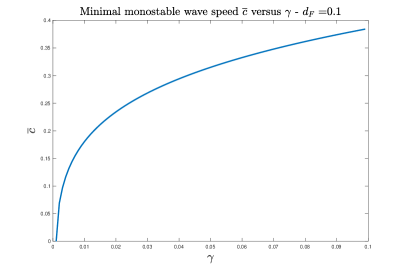
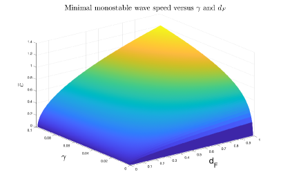
Figure 1: Variations of the minimal wave speed $\overline{c}$ of the monostable traveling wave solution of system (12)-(17) connecting the elimination equilibrium 0 and the positive equilibrium $E^{*}$ when no SIT occurs, i.e. $M_{T}=0$. (a): the evolution of $\overline{c}$ versus $\gamma$ for a given value of $d_{F}$, namely $d_{F}=0.1$; (b): the evolution of $\overline{c}$ versus $\gamma$ and $d_{F}$.

In Fig. 2, page 2, we represent the invasive monostable wave solution of system (12)-(17) when there is no SIT control. Only the immature stage (Fig. 2-(a)) and fertilized and eggs-laying female (Fig. 2-(b)) mosquito components are displayed. The wave connects the unstable elimination equilibrium 0 and the stable wild equilibrium, ${\bf{E}}^{*}\approx(18950,5412,7429)^{\prime}$. Starting with a local distribution of wild mosquitoes, transient states first take place (e.g. at times 25, 50, 75 and 100 days in figure 2). After these transient states, the invasive monostable wave occurs (e.g. at times 125, 150, 175 and 200 days in Fig. 2, page 2). Thanks to the previous estimate, the speed of the monostable traveling wave is $\overline{c}\approx 0.362$ km/day. In the long term dynamic, we have a complete invasion of the spatial domain (e.g. between times 375 and 400 days in figure 2).

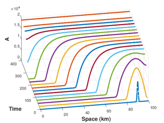
(a)

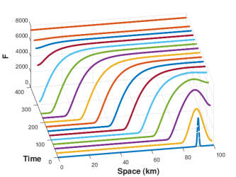
(b)

Figure 2: Invasive monostable wave solution when there is no SIT release. The wave connects the unstable elimination equilibrium, 0, to the stable wild equilibrium, ${\bf{E}}^{*}$.

In the next section, we assume that SIT releases are considered. We further assume two initial configurations: a partial invasion of the spatial domain and a full invasion of the spatial domain.

4.2 With SIT control - $M_{T}>0$

We now consider the monostable wave solution (e.g. $t=170$ days in Fig. 2, page 2) as the initial setting. Therefore, there exists a vector/pest-free subdomain and a vector/pest-persistent subdomain. We introduce sterile males, $0<M_{T}<M_{T_{1}}$, such that $\bf{0}$ becomes LAS, introducing a strong Allee effect. We know that Allee effects can slow or even reverse traveling wave solutions: this is exactly what we observe in the following simulations.

In Figs. 3(a-b-c), page 3, we observe that the introduction of sterile males, i.e. $M_{T}=1000,2000,3000$ respectively, slows down the traveling wave speed and thus the invasion: see also Fig. 4, page 4, where numerical estimates of the traveling wave speed are provided. This shows that even if the SIT-threshold is not reached but the amount of sterile males to be released is sufficient, it can help to delay a pest/vector invasion.

However, there exists a critical value $M_{T}^{c}$, close to $M_{T}$, such that the traveling wave stops or reverses leading to elimination in the (very) long term (see Fig. 3(d) and Fig. 4). However, since $M_{T}^{c}$ is close to $M_{T_{1}}$, it is more interesting to release above $M_{T_{1}}$ since we know that $\bf{0}$ is GAS, such that the system will reach elimination more or less quickly depending on whether $M_{T}$ is larger or much larger than $M_{T_{1}}$, like $M_{T}=k\times M_{T_{1}}$ with $k>1$.

To avoid the permanent use of massive releases, we can also use the massive and small releases strategy developed in [3]. Indeed, when $M_{T}>0$, the SIT problem has three equilibria, $\bf{0}$, $\bf{E}_{1}$, and $\bf{E}_{2}$, where $\bf{E}_{1}$ is unstable while $\bf{0}$ and $\bf{E}_{2}$ are LAS, and such that $[\bf{0},\bf{E}_{1})$ belongs to the basin of attraction of $\bf{0}$ and $\bf{E}_{1}$ is defined for a given value of $M_{T}$, say $100$ [3]. Thus, the massive-small strategy consists of releasing first sterile males massively, i.e. $M_{T}=k\times M_{T_{1}}$, with $k>1$, in order to reach the parallelepiped $[\bf{0},\bf{E}_{1})$. Then, once $[\bf{0},\bf{E}_{1})$ is reached, we can switch from massive releases to small releases, $M_{T}=100$, and use the AS of $\bf{0}$ within $[\bf{0},\bf{E}_{1})$ to drive the wild population to elimination. This is feasible but it requires to release the sterile males homogeneously over the treated area.

However, the previous strategies are unrealistic in the field: it is impossible to treat large areas using (permanent) massive releases. Also, some areas may be difficult to reach in order to release sterile males homogeneously. In general a barrier or a corridor strategy is recommended, but the difficulty is to define the width of this corridor and also the right strategy to avoid the risk of pest/mosquito emergence within the untreated area that has to be protected.

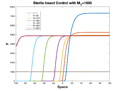
(a)

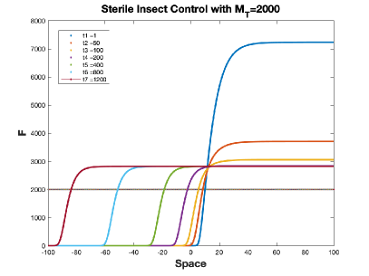
(b)

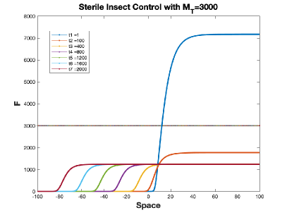
(c)

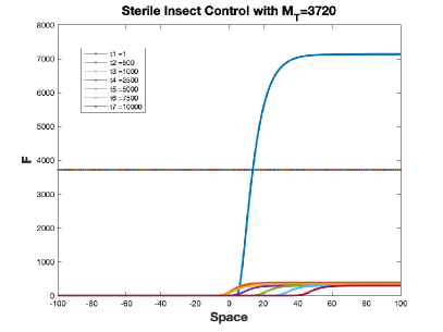
(d)

Figure 3: Long term dynamics for several values of SIT releases when $0<M_{T}<M_{T_{1}}$

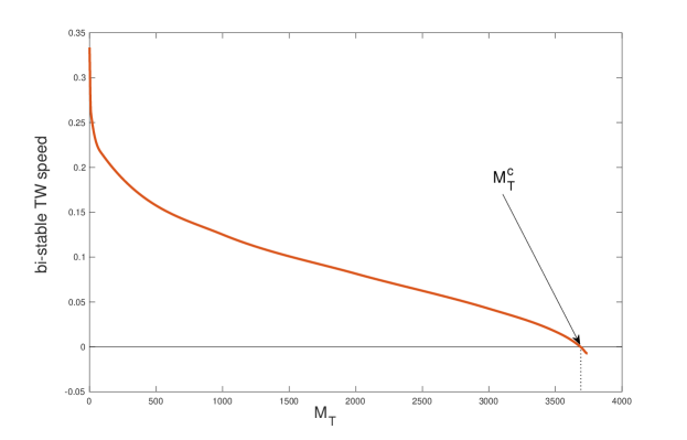
Figure 4: Numerical estimates of the bistable traveling wave speed when $0<M_{T}<M_{T_{1}}$

4.3 The “corridor/barrier strategy” - blocking wave

Following [16, 22], we want to apply the control strategy developed and studied in [3], combining massive releases (locally) and small releases to stop the invasion of mosquitoes or pest and eventually to push them back. In fact we use the location of the front linking $\bf{0}$ and $\bf{E}_{2}$, to define a sufficiently large corridor, where massive releases, $M_{T}>M_{T_{1}}$, will be used, while the free area will be treated with small releases only.

Here, consider that we want to protect an area delimited by $0$ and $x_{\min}$ from an invasion of pest/mosquitoes using SIT releases. To do that we release a massive number of sterile males within corridor $[x_{\min},x_{\max}]$ in order to block the invasive front. Within $[x_{\min},x_{\max}]$, we release $1.1\times M_{T_{1}}$ sterile males, while in $[0,x_{\min})$, we release only $M_{T_{1}}/100$ sterile males, which leads to define the unstable equilibrium. When $d_{F}=0.05$ or $d_{F}=0.1$, we choose $x_{\min}$ and $x_{\max}$ such that $x_{\max}-x_{\min}=20$ km: see Figs. 5 and 6, page 5. Thus clearly, for the same amount for massive releases, for different, but close, values of $d_{F}$, the starting dates of the corridor control is crucial: $300$ for $d_{F}=0.05$, and $200$ for $d_{F}=0.1$. As seen, the strategy we have developed in [3] is still very suitable when considering the spatial component.

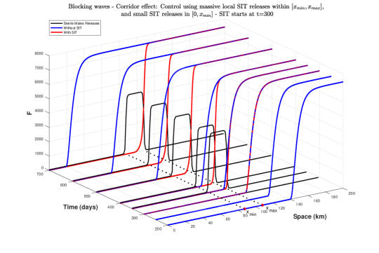
Figure 5: Control strategy using a 20 km corridor to block mosquito/pest invasion using massive releases within the corridor, and small releases on the left side of the corridor. SIT starting date: $t=300$. We consider $\gamma=0.08$, $d_{F}=0.05$, $d_{M}=0.05$, $M_{T}=1.1\times M_{T_{1}}$. The rest of the parameters are given in Table 2.

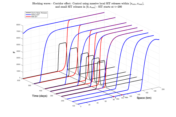
Figure 6: Control strategy using a 20 km corridor to block mosquito/pest invasion using massive releases within the corridor, and small releases on the left side of the corridor. SIT starting date: $t=200$. We consider $\gamma=0.08$, $d_{F}=0.1$, $d_{M}=0.05$, $M_{T}=1.1\times M_{T_{1}}$. The rest of the parameters are given in Table 2.

The same strategy can be used to stop and push back the wild pest/mosquito wave. Indeed, once the wave is blocked, it might be possible to move to the right the corridor, like a “traveling carpet”. Using the same parameters and also the same corridor width, but releasing $1.8\times M_{T_{1}}$ sterile males inside $[x_{\min}(t),x_{\max}(t)]$ we obtain the simulations in Fig. 7, page 7. The dotted lines indicate the original location of the control to block the wave. Then, the corridor is moved once, at the left-end, $x_{\min}(t)$ of the corridor, we have $(E,M,F)^{\prime}<(E_{1},M_{1},F_{1})^{\prime}$.

It is possible to push back faster the mosquito/pest traveling wave by expanding the corridor width from $20$ km to $40$ km (see Fig. 8 page 8), for instance. The counterpart is, of course, to release a larger number of sterile males within the corridor. This shows that a relationship might exists between the size of the massive releases, the corridor depth and the duration of the massive releases. These parameters can also be constrained by the sterile males production constraint.

Last but not least, the same strategy could be used to treat a whole domain still invaded by a pest or mosquito and to get ride of them after longtime treatment. Of course, in order to avoid a re-invasion, it will be necessary to continue the SIT treatment, with small releases, in order to maintain the wild population under a given threshold, $\bf{E}_{1}$, for instance.

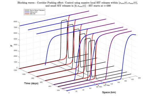
Figure 7: Dynamic Control strategy using a 27 km corridor to block and push back mosquito/pest invasion using massive releases within the corridor, and small releases on the left side of the corridor. We consider $\gamma=0.08$, $d_{F}=0.1$, $d_{M}=0.05$, and $M_{T}=1.8\times M_{T_{1}}$. The rest of the parameters are given in Table 2.

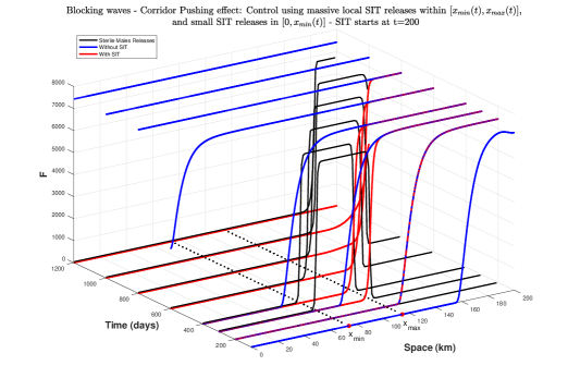
Figure 8: Dynamic Control strategy using a 40 km corridor to block and push back the invasion of mosquitoes using massive releases within the corridor, and small releases on the left side of the corridor. We consider $\gamma=0.08$, $d_{F}=0.1$, $d_{M}=0.05$, $M_{T}=1.8\times M_{T_{1}}$. The rest of the parameters are given in Table 2.

The previous “corridor” and “barrier” strategies could also be used against other pest, like Ceratitis capitata (“medfly”) or Bactrocera dorsalis (“oriental fruit fly”). Indeed, C. capitata was removed from invaded areas in southern Mexico, and for thirty years a sterile fly barrier across Guatemala has maintained Mexico and the USA medfly-free. The barrier strategy is still used successfully against screwworms, Cochliomyia hominivorax (Coquerel), at the border of Panama and Colombia, protecting North-America from this damaging pest [24]. However, the objectives are now to use SIT more locally to protect or free (from pest) specific places instead of treating large area.

5 Conclusion

In this work, we have extend the temporal model studied in [3] to a spatio-temporal one. In order to show the existence of traveling wave solutions we have also extended results from [11]. This allows us to show that when $0\leq M_{T}<M_{T_{1}}$, on the whole area, a monotone wavefront may exist, connecting $\bf{0}$ with a positive equilibrium. When SIT control is such that $M_{T}^{c}<M_{T}<M_{T_{1}}$, on the whole area, then we showed, numerically, that the population can be driven to elimination. However, for realistic use, we have considered the strategy of massive-small releases studied in [3], using massive releases in a spatial corridor of sufficient depth to block the front of the traveling wave, and using small releases within the targeted area, i.e. the pest/vector free area. We show that this strategy can be successful to block the invasion and eventually can also be used, using a “dynamic corridor”, to push back the pest or the vector and thus free invaded area.

Theoretically, the corridor case is still an open problem. In particular, in future studies, it would be useful to derive a relationship between the width of the corridor, the size of the massive releases, the sterile insects manufacturing capacity, etc. Such a result would be useful in order to implement appropriate sterile male release strategies.

Last but not least, our work takes place within several SIT projects in la Réunion (a French tropical island, located in the Indian Ocean, east from Madagascar and southwest from Mauritius island) and Corsica (a French island in the Mediterranean Sea, southeast of France and west of Italy), for which field experiments, and in particular field releases, are expected. We hope that our results will help to improve the release strategies and thus the impact of SIT, in combination with other biocontrol strategies, using mechanical control, prophylaxis, etc.

Appendix A Some results on reaction-diffusion (RD) systems

Let us consider the abstract Cauchy problem:

$$\left\{\begin{array}[]{l}\displaystyle\frac{du}{dt}+Au=F(u),\\ u(0)=u_{0}\end{array}\right.$$ (27)

where for $B=C_{ub}(\mathbb{R})$,

$$\left\{\begin{array}[]{l}D(A)=\{f\in B:f^{\prime\prime}\quad\mbox{exists},\quad f^{\prime}\in B,\quad f^{\prime\prime}\in B\},\\ Au=-du^{\prime\prime}.\end{array}\right.$$ (28)

Systems of reaction-diffusion equations assume also the form (27) where $u=(u_{1},u_{2},...,u_{n})$, $F=(F_{1},F_{2},...,F_{n})$, $d=diag(d_{1},d_{2},...,d_{n})$ with $d_{i}>0$, for $i=1,2,...,n$ and
$\displaystyle\frac{\partial^{2}u}{\partial x^{2}}:=\left(\displaystyle\frac{\partial^{2}u_{1}}{\partial x^{2}},\displaystyle\frac{\partial^{2}u_{2}}{\partial x^{2}},...,\displaystyle\frac{\partial^{2}u_{n}}{\partial x^{2}}\right)$. The corresponding Gauss-Weierstrass $C_{0}-$semigroup
$S(t)=(S_{1}(t),S_{2}(t),...,S_{n}(t))$ is defined on a Banach space $B=B_{1}\times...\times B_{n}$ by $S_{i}(0)=I$ and for $t>0$

$$\begin{array}[]{ccl}(S_{i}(t)f)(x)&=&\displaystyle\frac{1}{\sqrt{4\pi d_{i}t}}\displaystyle\int_{\mathbb{R}}\exp\left(-\displaystyle\frac{(x-y)^{2}}{4d_{i}t}\right)f(y)dy\qquad(x\in\mathbb{R},f\in B_{i})\\ &=&(G_{t,i}\star f)(x)\end{array}$$ (29)

where

$$G_{t,i}(x)=\displaystyle\frac{1}{\sqrt{4\pi d_{i}t}}\exp\left(-\displaystyle\frac{x^{2}}{4d_{i}t}\right),\quad i=1,2,...,n.$$

In the case where some (but not all) diffusion coefficient $d_{i_{0}}=0$, the corresponding operator in the Gauss-Weierstrass $C_{0}-$semigroup is taken as (Rauch and Smoller (1978) [21]) $S_{i_{0}}(0)=I$ and for $t>0$

$$\begin{array}[]{ccl}(S_{i_{0}}(t)f)(x)&=&(G_{t,i_{0}}\star f)(x)=f(x)\end{array}$$ (30)

with $G_{t,i_{0}}(x)=\delta(x)$. $\delta$ is the Dirac distribution and is defined by

$$\delta(x)=\left\{\begin{array}[]{cl}0,&x\neq 0\\ +\infty,&x=0\end{array}\right.$$

with

$$\int_{\mathbb{R}}\delta(y)dy=1.$$

Appendix B Proof of Lemma 1

Recall that $w=(A,M,F)^{\prime}$ and

$$H(w)=\left(\phi F-(\gamma+\mu_{A,1}+\mu_{A,2}A)A,(1-r)\gamma A-\mu_{M}M,\displaystyle\frac{M}{M+M_{T}}r\gamma A-\mu_{F}F\right)^{\prime}.$$

Following [26, pages 210-211], one has

$$\begin{array}[]{l}G=-A,\quad\left.\nabla G\cdot H\right|_{A=0}=-\phi F\leq 0\quad\mbox{in}\quad\Gamma_{\mathcal{R}\leq 1}\cup\Gamma_{\mathcal{R}>1},\quad\mbox{so}\quad A\geq 0.\\ G=-M,\quad\left.\nabla G\cdot H\right|_{M=0}=-(1-r)\gamma A\leq 0\quad\mbox{in}\quad\Gamma_{\mathcal{R}\leq 1}\cup\Gamma_{\mathcal{R}>1},\quad\mbox{so}\quad M\geq 0.\\ G=-F,\quad\left.\nabla G\cdot H\right|_{F=0}=-\dfrac{M}{M+M_{T}}r\gamma A\leq 0\quad\mbox{in}\quad\Gamma_{\mathcal{R}\leq 1}\cup\Gamma_{\mathcal{R}>1},\quad\mbox{so}\quad M\geq 0.\\ \end{array}$$

1. Assume that $\mathcal{R}\leq 1$ or equivalently $\dfrac{r\gamma}{\mu_{F}}\leq\dfrac{\gamma+\mu_{{A,1}}}{\phi}$.

   $$\begin{array}[]{l}G=M-\dfrac{(1-r)\gamma}{\mu_{M}}k_{1},\quad\left.\nabla G\cdot H\right|_{M=\dfrac{(1-r)\gamma}{\mu_{M}}k_{1}}=(1-r)\gamma(A-k_{1})\leq 0\quad\mbox{in}\quad\Gamma_{\mathcal{R}\leq 1},\\ \quad\mbox{so}\quad M\leq\dfrac{(1-r)\gamma}{\mu_{M}}k_{1}.\\ G=F-\dfrac{r\gamma}{\mu_{F}}k_{1},\quad\left.\nabla G\cdot H\right|_{F=\dfrac{r\gamma}{\mu_{F}}k_{1}}\leq r\gamma(A-k_{1})\leq 0\quad\mbox{in}\quad\Gamma_{\mathcal{R}\leq 1},\quad\mbox{so}\quad F\leq\dfrac{r\gamma}{\mu_{F}}k_{1}.\\ G=A-k_{1},\quad\left.\nabla G\cdot H\right|_{A=k_{1}}\leq\phi\left(F-\dfrac{\gamma+\mu_{{A,1}}}{\phi}k_{1}\right)\leq\phi\left(F-\dfrac{r\gamma}{\mu_{F}}k_{1}\right)\leq 0\quad\mbox{in}\quad\Gamma_{\mathcal{R}\leq 1},\\ \quad\mbox{so}\quad A\leq k_{1}.\\ \end{array}$$

2. Assume that $\mathcal{R}>1$. Hence the positive wild equilibrium $E^{*}=(A^{*},M^{*},F^{*})^{\prime}$ is defined. Note that $M^{*}=\dfrac{(1-r)\gamma}{\mu_{M}}A^{*}$ and $F^{*}=\dfrac{r\gamma}{\mu_{F}}A^{*}$. One has

   $$\begin{array}[]{l}G=M-k_{2}M^{*},\quad\left.\nabla G\cdot H\right|_{M=k_{2}M^{*}}=(1-r)\gamma(A-k_{2}A^{*})\leq 0~{}\mbox{in}~{}\Gamma_{\mathcal{R}>1},~{}\mbox{so}~{}M\leq k_{2}M^{*}.\\ G=F-k_{2}F^{*},\quad\left.\nabla G\cdot H\right|_{F=k_{2}F^{*}}\leq r\gamma(A-k_{2}A^{*})\leq 0\quad\mbox{in}\quad\Gamma_{\mathcal{R}>1},\quad\mbox{so}\quad F\leq k_{2}F^{*}.\\ G=A-k_{2}A^{*},\quad\left.\nabla G\cdot H\right|_{A=k_{2}A^{*}}=\phi\left(F-(\gamma+\mu_{{A,1}}+\mu_{A,2}A^{*})A^{*}\right)\\ \hskip 170.71652pt=\phi\left(F-k_{2}F^{*}\right)+\mu_{A,2}k_{2}A^{*}(1-k_{2})\\ \hskip 170.71652pt\leq 0\quad\mbox{in}\quad\Gamma_{\mathcal{R}>1},~{}\mbox{so}~{}A\leq k_{2}A^{*}.\\ \end{array}$$

This ends the proof of the Lemma.

References

- [1] R. Anguelov, Y. Dumont, and J. Lubuma. Mathematical modeling of sterile insect technology for control of anopheles mosquito. Comput. Math. Appl., 64:374–389, 2012.
- [2] R. Anguelov, Y. Dumont, and J. Lubuma. On nonstandard finite difference schemes in biosciences. AIP Conf. Proc., 1487:212–223, 2012.
- [3] R. Anguelov, Y. Dumont, and I.V. Yatat Djeumen. Sustainable vector/pest control using the permanent sterile insect technique. Mathematical Methods in the Applied Sciences, pages 1–22, 2020.
- [4] M. Soledad Aronna and Yves Dumont. On nonlinear pest/vector control via the sterile insect technique: Impact of residual fertility. Bulletin of Mathematical Biology, 82(8):110, Aug 2020.
- [5] R. Asadi, R. Elaini, R. Lacroix, T. Ant, A. Collado, L. Finnegan, P. Siciliano, A. Mazih, and M. Koukidou. Preventative releases of self-limiting ceratitis capitata provide pest suppression and protect fruit quality in outdoor netted cages. International Journal of Pest Management, 66(2):182–193, 2020.
- [6] P.-A. Bliman, D. Cardona-Salgado, Y. Dumont, and O. Vasilieva. Implementation of control strategies for sterile insect techniques. Mathematical Biosciences, 314:43 – 60, 2019.
- [7] Anne Tuiskunen Bäck and Åke Lundkvist. Dengue viruses – an overview. Infection Ecology & Epidemiology, 3(1):19839, 2013. PMID: 24003364.
- [8] C. Dufourd and Y. Dumont. Impact of environmental factors on mosquito dispersal in the prospect of sterile insect technique control. Computers & Mathematics with Applications, 66(9):1695 – 1715, 2013. BioMath 2012.
- [9] V. A. Dyck, J. Hendrichs, and A. S. Robinson. The Sterile Insect Technique, Principles and Practice in Area-Wide Integrated Pest Management. Springer, Dordrecht, 2006.
- [10] T. Oleron Evans and S.R. Bishop. A spatial model with pulsed releases to compare strategies for the sterile insect technique applied to the mosquito aedes aegypti. Mathematical Biosciences, 254:6 – 27, 2014.
- [11] J. Fang and X. Zhao. Monotone wavefronts for partially degenerate reaction-diffusion systems. J. Dyn. Diff. Equat., 21:663–680, 2009.
- [12] C.P. Ferreira, H.M. Yang, and L. Esteva. Assessing the suitability of sterile insect technique applied to aedes aegypti. Journal of Biological Systems, 16(04):565–577, 2008.
- [13] N. G. Gratz. Critical review of the vector status of aedes albopictus. Medical and Veterinary Entomology, 18(3):215–227, 2004.
- [14] E. F. Knipling. Possibilities of insect control or eradication through the use of sexually sterile males. Journal of Economic Entomology, 48(4):459 – 462, 1955.
- [15] S. Seirin Lee, R.E. Baker, E.A. Gaffney, and S.M. White. Modelling aedes aegypti mosquito control via transgenic and sterile insect techniques: Endemics and emerging outbreaks. Journal of Theoretical Biology, 331:78 – 90, 2013.
- [16] M.A. Lewis and P. Van Den Driessche. Waves of extinction from sterile insect release. Mathematical Biosciences, 116(2):221 – 247, 1993.
- [17] B. Li, F.H. Weinberger, and M. Lewis. Spreading speeds as slowest wave speeds for cooperative systems. Math. Biosci., 196(1):82 – 98, 2005.
- [18] J.D. Logan. An introduction to nonlinear partial differential equations, second edition. John Wiley and Sons, Inc., 2008.
- [19] V.S. Manoranjan and P. Van Den Driessche. On a diffusion model for sterile insect release. Mathematical Biosciences, 79(2):199 – 208, 1986.
- [20] R. Marsula and C. Wissel. Insect pest control by a spatial barrier. Ecological Modelling, 75-76:203 – 211, 1994. State-of-the-Art in Ecological Modelling proceedings of ISEM’s 8th International Conference.
- [21] J. Rauch and J. Smoller. Qualitative theory of the fitzhugh-nagumo equations. Advances in Mathematics, 27(1):12 – 44, 1978.
- [22] S. Seirin Lee, R. E. Baker, E.A. Gaffney, and S.M. White. Optimal barrier zones for stopping the invasion of aedes aegypti mosquitoes via transgenic or sterile insect techniques. Theoretical Ecology, 6(4):427–442, Nov 2013.
- [23] S.P. Sinkins. Wolbachia and cytoplasmic incompatibility in mosquitoes. Insect Biochemistry and Molecular Biology, 34(7):723 – 729, 2004. Molecular and population biology of mosquitoes.
- [24] S.R. Skoda, P.L. Phillips, A. Sagel, and M.F. Chaudhury. Distribution and Persistence of Sterile Screwworms (Diptera: Calliphoridae) Released at the Panama–Colombia Border. Journal of Economic Entomology, 110(2):783–789, 02 2017.
- [25] H. Smith. Monotone Dynamical Systems. AMS, 1995.
- [26] J. Smoller. Shock Waves and reaction-diffusion systems. Springer, 1983.
- [27] M. Strugarek, H. Bossin, and Y. Dumont. On the use of the sterile insect technique or the incompatible insect technique to reduce or eliminate mosquito populations. Applied Mathematical Modelling, 68:443 – 470, 2019.
- [28] R. Tyson, H. Thistlewood, and G.J.R. Judd. Modelling dispersal of sterile male codling moths, cydia pomonella, across orchard boundaries. Ecological Modelling, 205(1):1 – 12, 2007.
- [29] Roger Vargas, Jaime Piñero, and Luc Leblanc. An overview of pest species of bactrocera fruit flies (diptera: Tephritidae) and the integration of biopesticides with other biological approaches for their management with a focus on the pacific region. Insects, 6(2):297–318, Apr 2015.
- [30] F.H. Weinberger, A.M. Lewis, and B. Li. Analysis of linear determinacy for spread in cooperative models. J. Math. Biol., 45(3):183–218, 2002.