Bridging the Gaps in Statistical Models of Protein Alignment

Abstract

This work demonstrates how a complete statistical model quantifying the evolution of pairs of aligned proteins can be constructed from a time-parameterised substitution matrix and a time-parameterised 3-state alignment machine. All parameters of such a model can be inferred from any benchmark data-set of aligned protein sequences. This allows us to examine nine well-known substitution matrices on six benchmarks curated using various structural alignment methods; any matrix that does not explicitly model a “time”-dependent Markov process is converted to a corresponding base-matrix that does. In addition, a new optimal matrix is inferred for each of the six benchmarks. Using Minimum Message Length (MML) inference, all 15 matrices are compared in terms of measuring the Shannon information content of each benchmark. This has resulted in a new and clear overall best performed time-dependent Markov matrix, MMLSUM, and its associated 3-state machine, whose properties we have analysed in this work. For standard use, the MMLSUM series of (log-odds) scoring matrices derived from the above Markov matrix, are available at https://lcb.infotech.monash.edu.au/mmlsum.
 

1 Introduction

Extant proteins diverge from their ancestors while tolerating considerable variation to their amino acid sequences [11]. Inferring and comparing trustworthy relationships between their sequences is a challenging task and, when done properly, provides a powerful way to reason about the macromolecular consequences of evolution [26].

Many biological studies rely on identifying homologous relationships between proteins. The details of those relationships are represented as correspondences (alignment) between subsets of their amino acids. Each such correspondence suggests the divergence of the observed amino acids arising from a common locus within the ancestral genome.

Although sequence comparison is a mature field, the fidelity of the relationships evinced by modern homology detection and alignment programs remains a function of the underlying models they employ to evaluate hypothesised relationships. Most programs utilise a substitution matrix to quantify amino acid interchanges. These matrices are parameterised on a numeric value that accounts for the extent of divergence/similarity between protein sequences (e.g. PAM-250 [16], BLOSUM-62 [19]).

Separately, the unaligned regions (gaps) of an alignment relationship are taken as insertions and deletions (indels), accumulated during sequence evolution. Separate gap-open and gap-extension penalties are widely felt to give plausible and sufficiently flexible models to quantify indels. However, mathematically reconciling the quantification of substitutions with that of indels remains contentious. Often the issue is simply avoided: previous studies have shown that the choices of which substitution matrix to use, at what threshold of divergence/similarity, and with what values for gap penalties, remain anecdotal, sometimes empirical, if not fully arbitrary [45, 17, 40]. Evaluation of the performance of popularly-used substitution matrices is hampered by the fact that different sequence comparison programs yield conflicting results [17, 7, 45, 9, 27]. Thus, as the field stands, it lacks an objective framework to assess how well the commonly-used substitution matrices perform for the task of comparison, without being impeded by ad hoc parameter choices.

To address these lacunae, we describe an unsupervised probabilistic and information-theoretic framework that uniquely allows us to:

1. compare the performance of existing amino acid substitution matrices, in terms of Shannon information content, without any need for parameter-fiddling,

2. infer improved stochastic (Markov) models of amino acid substitutions that demonstrably outperform existing substitution matrices, and

3. infer Dirichlet distributions accompanying the above Markov models, which provide a unified way to address amino acid insertions and deletions in probabilistic terms.

Specifically, for any given collection of benchmark alignments, our framework uses the Bayesian Minimum Message Length (MML) criterion [46, 2] to estimate the Shannon information content [37] of that collection, measured in bits. It is computed as the shortest encoding length required to compress losslessly all sequence pairs in the collection using their stated alignment relationships. This measure of Shannon information is based on rigorous probabilistic models that capture protein evolution (substitutions and indels). Parameters are inferred unsupervised (i.e. automatically) by maximising the lossless compression that can be gained from the collection. In general, Shannon information is a fundamental and measurable property of data, and has had effective use in studies involving biological macromolecules [3, 39, 1].

Central to our information-theoretic framework is a stochastic matrix describing a Markov chain, which models the probabilities of interchanges between amino acids as a function of time (of divergence). It works in concert with corresponding time-specific Dirichlet probability distributions that are learnt from the collection to model the parameters of the alignment finite-state machine, which is used to quantify the (information-measure of) complexity of alignments. This handling of alignment complexity over time-dependent 3-state ($\texttt{match},\texttt{insert},$ and delete) machine models overcomes any ad hoc decisions about gap penalty functions and costs. Crucially, all probabilistic parameters in this framework are automatically inferred by optimising the underlying MML criterion. Using this framework we are also able to infer new, and demonstrably improved models of amino acid evolution.

Furthermore, our framework enables the conversion of existing substitution matrices to corresponding stochastic matrices with high-fidelity, even those that do not explicitly model amino acid interchanges as a Markov process. This provides a way to directly and objectively compare the performance of substitution matrices without any parameter-tuning, and measure their respective lossless encoding lengths required to compress the same collection of benchmark alignments. To the best of our knowledge, all the above features are unique to the work presented here.

In the section below, we compare and contrast an extensive range of widely used substitution matrices introduced over the past four decades. We demonstrate the improvement of a new substitution matrix (MMLSUM) inferred by our MML framework and analyse the properties of MMLSUM. Section 3 gives a mathematical overview of our framework, with details explained in supplementary Section S1.

2 Results and Discussion

We consider nine well-known substitution matrices and new matrices inferred in this work. In order of publication, the former are: PAM [16], JTT [22], BLOSUM [19], JO [21], WAG [49], VTML [30], LG [24], MIQS [50], and PFASUM [23]. The matrices are compared on six different alignment benchmarks (Section 3.3) which are curated using diverse structural alignment programs. Further, for each benchmark, our MML framework is able to infer a stochastic matrix that best explains the benchmark. We compare the MML-inferred matrices against the existing matrices across the 6 benchmark collections.

The organization of this section is as follows: Section 2.1 describes the composition of the benchmarks. Section 2.2 presents the performance of all the matrices across each benchmark using the objective measure of Shannon information content when losslessly compressing the same benchmark alignment collection. From this we identify the most-generalisable matrix among the set of MML-inferred substitution matrices on various benchmarks, that outperforms the other matrices – we term this matrix MMLSUM. Section 2.3 analyses in detail MMLSUM, the best substitution model inferred here, for its characteristics including aspects of physicochemical and functional properties that the matrix captures, its relationship with expected change in amino acids as a function of divergence time, and the properties of gaps that can be derived from the companion probabilistic models that work with MMLSUM, amongst others.

2.1 Composition of alignment benchmarks

Table 1: Composition of alignment benchmarks used in this work.

Benchmark		Num. of seq.pairs	Num. of matches	Num. of inserts	Num. of deletes	Avg. seq. ID
Name (Abbrv.)	Curated with structural aligner
HOMSTRAD	MNYFIT, STAMP, COMPARER	8323	1,311,478	96,911	98,810	35.1%
MATTBENCH	MATT	5286	826,506	177,401	177,789	19.4%
SABMARK-Sup	SOFI, CE	19,092	1,750,440	848,859	861,344	15.2%
SABMARK-Twi	SOFI, CE	10,667	694,954	515,318	527,188	8.4%
SCOP1	DALI	56,292	8,663,652	1,407,988	1,373,882	25.5%
SCOP2	MMLIGNER	59,092	8,145,678	1,673,687	1,653,531	24.8%

Table 1 summarises the six alignment benchmarks in terms of the total number of sequence-pairs (and their corresponding alignments) that each collection contains, the number of observed $\{\texttt{match}$, insert, $\texttt{delete}\}$ states in their alignments, and their observed average sequence identity.

The distributions of sequence identity observed in each benchmark are shown in supplementary Fig. SF2. HOMSTRAD covers a wide range of sequence relationships. In comparison, SABMARK-Sup and MATTBENCH contain alignments of distant sequence-pairs. SABMARK-Twi contains alignments of sequences that have diverged into the ‘midnight zone’ where the detectable sequence signal is extremely feeble. Finally, the largest benchmark we use contains 59,092 unique sequence-pairs sampled from the superfamily and family levels of SCOP [31]. These pairs were aligned separately using DALI [20] and MMLigner [12] structural alignment programs to obtain SCOP1 and SCOP2 benchmarks, respectively (Section 3.3).

Collectively, all six benchmarks cover varying distributions of sequence relationships, whose alignments were curated using diverse structural alignment programs (second column of Table 1). This diversity of chosen benchmarks minimises the possibility of introducing any systematic bias to the evaluation of models of amino acid substitution.

2.2 Shannon information content of benchmarks

The lossless encoding length is estimated for each benchmark using the MML framework described in Section 3. The framework quantifies the Shannon information content of the benchmark, measured in bits, under varying models of amino acid substitution. That is, for each benchmark, the encoding scheme has a choice of either employing an existing substitution matrix (in its stochastic matrix form – see section Section 3.7), or automatically inferring a new stochastic matrix optimal to that collection.

Further, using the notations described in Section 3.2, for a stochastic matrix $\mathbf{M}$ chosen to losslessly compress all the sequence-pairs in a specific alignment benchmark $\mathbf{D}{}$, all the other models involved in this MML information-theoretic framework, i.e. $\{\mathbf{P},\boldsymbol{\alpha},\mathbf{\Theta},\tau\}$ (Section 3.2), are automatically-inferred (optimised) for $\mathbf{M}$ on each benchmark $\mathbf{D}{}$ under the MML criterion.

Table 2 presents the lengths of the shortest encoding (i.e. Shannon information) using each of the 15 matrices (9 existing; 6 inferred) to explain each of the six benchmarks.

Table 2: Shannon information content (in bits) to losslessly encode each benchmark by varying the substitution matrices. The rank order of their performance is reported in each column within parentheses (smaller lossless encoding length = better rank). Best encoding length for each benchmark is highlighted in bold blue font. All other parameters are inferred (optimised) by the MML framework for the matrix chosen to losslessly compress each benchmark.

Benchmark $\rightarrow$ (D)	HOMSTRAD	MATTBENCH	SABMARK-Sup	SABMARK-Twi	SCOP1	SCOP2
Matrix ($M$) $\downarrow$	Shannon information content using existing substitution matrices (and its rank across all matrices)
PAM (1978)	11531556.4 (15)	9143136.9 (15)	23574085.5 (15)	11310226.0 (15)	84925406.9 (15)	82757945.5 (15)
JTT (1992)	11481203.2 (14)	9072068.6 (13)	23450831.6 (13)	11251914.3 (13)	84353986.5 (13)	82218532.0 (13)
BLOSUM (1992)	11437552.8 (10)	9037049.8 (08)	23373908.1 (07)	11228043.6 (06)	84174710.8 (11)	81995179.3 (10)
JO (1993)	11476518.5 (13)	9118266.0 (14)	23501361.5 (14)	11290056.3 (14)	84567477.8 (14)	82405562.0 (14)
WAG (2001)	11419186.0 (05)	9052722.9 (12)	23400017.0 (11)	11243242.0 (12)	84141633.8 (09)	81996154.3 (11)
VTML (2002)	11423498.2 (07)	9035903.4 (07)	23377505.0 (08)	11230624.1 (08)	84075908.5 (07)	81925302.7 (07)
LG (2008)	11464263.6 (12)	9049040.6 (11)	23411713.3 (12)	11235389.2 (09)	84255656.9 (08)	82090289.0 (12)
MIQS (2013)	11422215.4 (06)	9040480.8 (10)	23385242.8 (10)	11236323.3 (10)	84076742.8 (12)	81927707.6 (08)
PFASUM (2017)	11412888.2 (02)	9039799.4 (09)	23379074.4 (09)	11236572.3 (11)	84040519.3 (04)	81902713.6 (06)
Matrix ($M$) $\downarrow$	Shannon information using MML-inferred matrices (and its rank across all matrices)
MML${}_{\text{{HOMSTRAD}}}$	11405604.7 (01)	9035317.6 (05)	23365151.2 (06)	11230184.9 (07)	84026302.3 (03)	81873575.9 (03)
MML${}_{\text{{MATTBENCH}}}$	11426344.1 (09)	9025882.4 (01)	23355215.8 (03)	11217219.1 (03)	84050927.4 (05)	81886796.3 (04)
MML${}_{\text{{SABMARK-Sup}}}$	11424135.9 (08)	9031315.9 (04)	23346025.4 (01)	11212252.7 (02)	84067892.9 (06)	81889152.3 (05)
MML${}_{\text{{SABMARK-Twi}}}$	11442781.7 (11)	9035720.5 (06)	23356054.5 (05)	11211360.9 (01)	84155701.5 (10)	81962307.9 (09)
MML${}_{\text{{SCOP1}}}$	11413295.6 (03)	9029682.8 (03)	23355235.9 (04)	11221295.6 (05)	83996796.0 (01)	81848381.0 (02)
MML${}_{\text{{SCOP2}}}$	11413725.3 (04)	9028667.52 (02)	23349826.8 (02)	11218205.6 (04)	83999536.4 (02)	81840654.6 (01)

Previously published matrices are arranged in chronological order of publication (rows). The last five rows show results for the stochastic matrices inferred from each benchmark.

To get an overall view of the performance of each matrix as a consensus over all benchmarks generated from individual ranks (shown within parentheses in each column of Table 2), we use a simple-yet-effective statistic: the (row-wise) sum of ranks of each matrix over all benchmarks, ranksum in short. Since this evaluation involves ranking 15 matrices over 6 benchmarks, the ranksum of any matrix is an integer between $6\times 1=6$ (best possible performance) and $6\times 15=90$ (worst possible performance).

Among the set of existing matrices, PAM ($\text{{ranksum}}={90}$) consistently gave the worst (i.e. longest) lossless encoding lengths across all benchmarks. This is anticipated, as PAM was derived in 1978 using the then available set of alignments. This is followed by the performance of JO ($\text{{ranksum}}={83}$), JTT ($\text{{ranksum}}={79}$), LG ($\text{{ranksum}}={64}$), WAG ($\text{{ranksum}}={60}$), MIQS ($\text{{ranksum}}={56}$), BLOSUM ($\text{{ranksum}}={52}$), VTML ($\text{{ranksum}}={44}$) and PFASUM ($\text{{ranksum}}={41}$). From these numbers it can be seen that, by and large, the previously published models of amino acid substitutions have improved over time. BLOSUM is among the earliest matrices (published in 1992) that outperforms several matrices that were proposed much later, and is only superseded in performance by VTML (published in 2002) and PFASUM (published recently in 2017), among the later matrices.

In comparison, the (stochastic) matrices inferred by our framework, specific to each benchmark, perform consistently better than previously-published substitution matrices. Indeed it is to be expected that the encoding length of any MML-inferred matrix that was optimised on a specific benchmark will outperform all other matrices on that benchmark – and this is precisely what is observed in Table 2 (see highlighted terms). However, the utility of any matrix lies in its ability to generalise to other benchmarks and perform well on those. The table above clearly demonstrates the ability of MML-inferred matrices to generalise and explain other benchmarks, far outperforming all existing ones. From the point of view of their ranksums: MML${}_{\texttt{SABMARK-Sup}}$ (i.e., the stochastic matrix inferred on SABMARK-Sup benchmark) gives $\text{{ranksum}}={26}$ across all benchmarks, while MML${}_{\texttt{MATTBENCH}}$ and MML${}_{\texttt{HOMSTRAD}}$ give $\text{{ranksum}}={25}$. The top two performers overall come from the matrices inferred on the two SCOP benchmarks, MML${}_{\texttt{SCOP1}}$ ($\text{{ranksum}}={18}$) and MML${}_{\text{SCOP2}}$ ($\text{{ranksum}}={15}$).

The sole outlier among the MML-inferred matrices was MML${}_{\text{SABMARK-Twi}}$ with $\text{{ranksum}}={42}$. As already stated (Section 2.1), SABMARK-Twi benchmark contains alignments of highly-diverged sequence-pairs (avg. seq. identity of 8.4%). Thus, the benchmark itself provides an extremely weak sequence signal to infer a stochastic matrix that can be generalised effectively to explain a wider range of sequence relationships that other benchmarks embody. But a noteworthy observation is that MML${}_{\texttt{SABMARK-Twi}}$ ($\text{{ranksum}}={42}$) is nearly in par with PFASUM ($\text{{ranksum}}={41}$) which was the best performer among the set of existing matrices. See supplementary Sections S2–S3 for an extended analysis and additional information.

Overall, the MML-inferred matrix from the SCOP2 benchmark (MML${}_{\text{{SCOP2}}}$) with a $\text{{ranksum}}={15}$ outperforms all other matrices. The is because SCOP2 benchmark is three times larger than SABMARK-Sup (seven times that of HOMSTRAD) and contains a wider range of sequence relationships than other benchmarks. Thus, all of our subsequent analyses will involve MML${}_{\text{{SCOP2}}}$ matrix – we will refer to it as MMLSUM (for MML subtitution matrix).

2.3 Analysis of MML substitution matrix (MMLSUM)

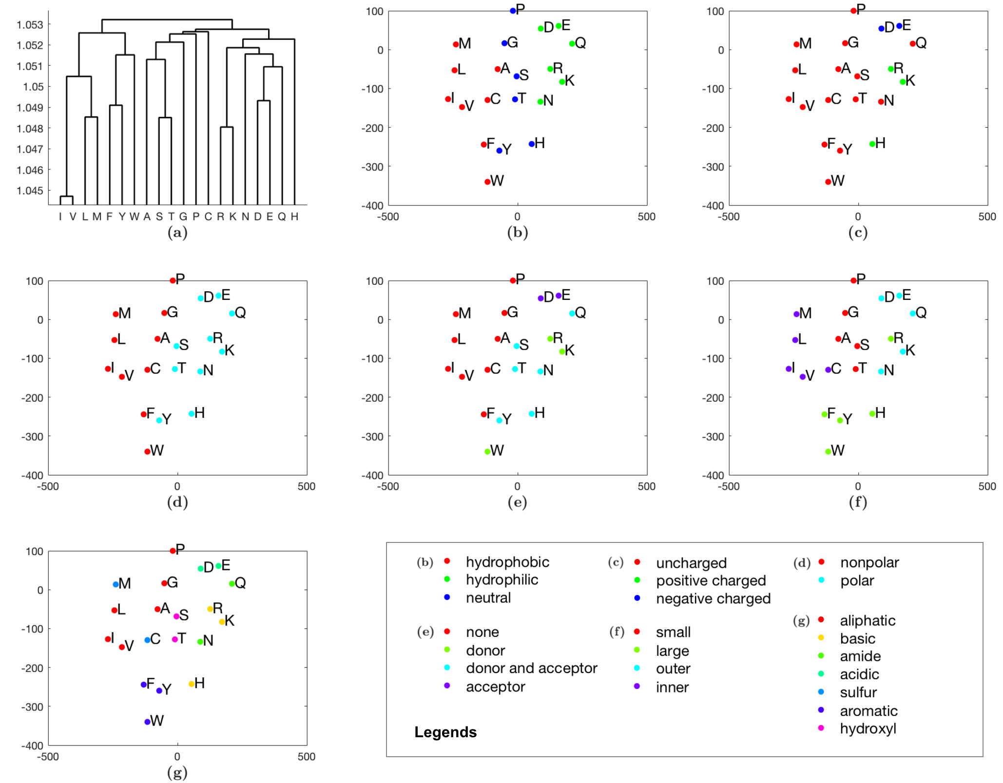
Figure 1: (a) Average-linkage clustering of amino acids generated from MMLSUM. (b)-(g) tSNE clustering of amino acids generated from MMLSUM. All plots have the same clustering, but coloured under different amino acid classification schemes based on: (b) hydropathy, (c) charge, (d) polarity, (e) Hydrogen donor or acceptor, (f) Swanson classification of amino acids [42] and (g) chemical properties (based on IMGT classification [25]). Refer to the legend for the colouring scheme in various subplots.

Amino acid clustering

Here we analyse groupings of amino acids implicit in MMLSUM. Fig. 1(a) gives a dendrogram generated using the average-linkage method on the MMLSUM base stochastic matrix (at $t=1$). We notice several important clusters that have been previously flagged as necessary for any reliable matrix quantifying amino acid substitutions [16]. The following groups can be identified:

• Hydrophobic amino acids Valine (V), Isoleucine (I), Leucine (L), and Methionine (M) cluster into a distinct clade.

• Aromatic amino acids Tryptophan (W), Tyrosine (Y), and Phenylalanine (F) group into another clade.

• Neutral amino acids Alanine (A), Serine (S), Threonine (T), Glycine (G) and Proline (P) group together.

• Large amino acids Arginine (R), Lysine (K), Asparagine (N), Aspartic acid (D), Glutamic acid (E), and Glutamine (Q) form a clade.

• The remaining two amino acids Histadine (H) and Cysteine (C) cluster apart from the rest.

To study the groupings observed more systematically and from a different point of view, we apply the technique of t-distributed stochastic neighbor embedding (tSNE) [43] to MMLSUM. tSNE performs a non-linear dimensionality reduction of high-dimensional feature space and gives visualizations that aid detection of clustering in lower dimensions [33]. Fig. 1(b)-(g) all show the same two-dimensional tSNE-visualisation of amino acids from MMLSUM, but each subplot colours the amino acids differently, based on widely-used amino acid classification schemes. These different schemes encompass the hydropathic character of amino acids, their charge, their polarity, their donor/acceptor roles in forming hydrogen bonds, their size and propensity for being buried/exposed, and their chemical constitution.

In Fig. 1(b)-(f), the visualization yields clearly separable amino acid groups on tSNE’s 2D embedding of MMLSUM. In Fig. 1(g) which deals with the classification based on the chemical characteristics of amino acids (as per IMGT [25]) the classes are mostly well-differentiated, barring a few outliers that include Histadine (H), Cysteine (C) and Asparagine (N) – we note that H and C were also outliers in the hierarchical clustering (cf. Fig. 1(a)).

Expected amino acid change and properties of gap lengths as a function of time of divergence

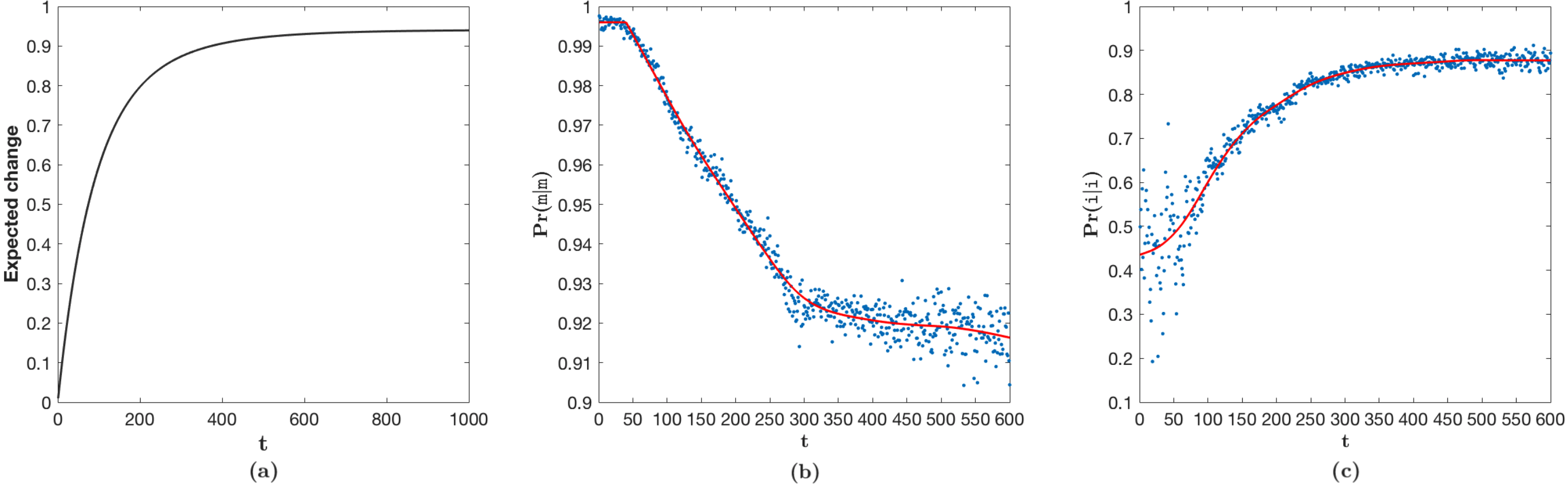
Figure 2: (a) Expected change of amino acids under the MMLSUM’s model as a function of divergence-time parameter $t$ (b) The variation of Pr($\text{{m}}|\text{{m}}$) when derived from the mean of the inferred time-dependent Dirichlet distributions accompanying MMLSUM. (c) Similarly, the variation of Pr($\text{{i}}|\text{{i}}$) estimate with $t$. The divergence time parameter $t$ is plotted in the range $[1,600]$, beyond which the amino acids have near-converged to the stationary distribution of MMLSUM (See supplementary Fig. SF6)

Fig. 2(a) shows the growth of expected change of amino acids implicit in MMLSUM as a function of time $t$. Previous studies [34] have shown that protein sequence relationships are most reliable when their sequence identity is $>40\%$ (or expected amino acid change $<60\%$). This corresponds approximately to the range $t\in[1,100]$ in Fig. 2(a). The ‘twilight zone’ of sequence relationships has been characterised by relationships sharing $[20-35]\%$ sequence identity (or $[65-80]\%$ change). This corresponds approximately to the range $t\in[125-200]$. Expected change of $90\%$ is reached at $t=400$ and increases very slowly thereafter ($94\%$ change at $t=1000$). (An extended analysis from the point of view of Kullback-Leibler divergence of individual amino acids with respect to the stationary distribution of MMLSUM is presented in supplementary Section S3.3.)

Further, unique to this framework is the optimal inference of “time” ($t$) dependent Dirichlet distributions that work in concert with the inferred stochastic matrix, MMLSUM. These distributions model time-specific state transition probabilities of the alignment 3-state machine over match (m), insert (i), and delete (d) states (see Fig. 4). Section 3.6 introduces the 9 transition probabilities involved in the alignment 3-state machine, of which three are free (Pr($\text{{m}}|\text{{m}}$), Pr($\text{{m}}|\text{{i}}$), and Pr($\text{{i}}|\text{{i}}$)), and the remaining dependent.

In the 3-state machine, the probability of moving from a match state to another match state (Pr($\text{{m}}|\text{{m}}$)) controls the run length of any block of matches in an alignment. The expected value of this run length, a geometrically distributed variable, is given by $\frac{1}{1-\text{Pr($\text{{m}}|\text{{m}}$)}}$. Also, the value $1-\text{Pr($\text{{m}}|\text{{m}}$)}$ gives the probability of a gap (i.e, a block of insertions or deletions of any length) starting at a given position in an alignment.

Fig. 2(b) plots the values of Pr($\text{{m}}|\text{{m}}$) derived from the mean values of the inferred Dirichlets for the match state. We observe that it remains nearly a constant ($\text{Pr($\text{{m}}|\text{{m}}$)}\approx 0.9958$) in the range of $t\in[1,40]$. This value corresponds to an expected run length of $\sim 238$ amino acids per block of matches. Sequence-pairs whose time parameter is in that range are closely-related, with $>67\%$ amino acids expected to be conserved (cf. Fig. 2(a)). The probability of opening a gap ($1-\text{Pr($\text{{m}}|\text{{m}}$)}=0.0042$) for sequence-pairs in this range is extremely small. Next, in the range $t\in[40,300]$ Pr($\text{{m}}|\text{{m}}$) decreases linearly with $t$. Comparing this range in Fig. 2(a), the expected change of amino acids drastically increases from $\sim 32\%$ to $\sim 87\%$. This correlates with the expected length of match-blocks dropping from $233$ amino acid residues to about $13$. Further, for $t\geq 300$, Pr($\text{{m}}|\text{{m}}$) decreases only gradually.

Similarly, the free parameter Pr($\text{{i}}|\text{{i}}$) (equalling Pr($\text{{d}}|\text{{d}}$) in the symmetric alignment state machine) controls the run lengths of indels. Fig. 2(c) gives values of Pr($\text{{i}}|\text{{i}}$) derived from the mean values of the inferred Dirichlets for the insert state. In the range $t\in[1,50]$ values of Pr($\text{{i}}|\text{{i}}$) are noisy because the probability of observing a gap is small. Hence, there are only few observations of gaps from which to estimate this parameter. However, in the range of $t\in[50,400]$ Pr($\text{{i}}|\text{{i}}$) grows from $0.5248$ to about $0.8431$, beyond which the probability flattens out at about $0.8759$ on average (expected gap length $\frac{1}{1-\text{Pr($\text{{i}}|\text{{i}}$)}}=\sim 8$ amino acid residues). The change of Pr($\text{{m}}|\text{{i}}$) with $t$ mirrors the behaviour of Pr($\text{{i}}|\text{{i}}$). This is because $\text{Pr($\text{{i}}|\text{{i}}$)}+\text{Pr($\text{{m}}|\text{{i}}$)}+\text{Pr($\text{{d}}|\text{{i}}$)}=1$, and Pr($\text{{d}}|\text{{i}}$) remains very small.

Function similarity and evolutionary distance

We analyse how functional similarity between the protein domain-pairs in the SCOP2 benchmark correlates with the automatically-estimated time (of divergence) parameter, under the MMLSUM model, for each of its $59,092$ sequence-pairs. (Refer supplementary Fig. SF5 for the distribution of the inferred set of time parameters.) For this, we employ the Gene Ontology (GO) [13] that provides function annotations for protein domains in three categories: (1) the ‘Biological Process’ (BP) they come from, (2) the ‘Molecular Function’ (MF) they exhibit, and (3) the ‘Cellular Component’ (CC) they belong to. Due to missing tags in the GO database, not all pairs could be considered for the analysis presented below: we considered only those domain-pairs where both their domains have one or more of the above categories tagged in the GO database. This resulted in 37,201 pairs for exploration of functional similarity at the level of BP, 48,215 pairs at the level of MF, and 31,594 at the level of CC.

The function-similarity between a domain pair is evaluated on a similarity measure involving the list of terms within each category as follows. Each domain is represented as a boolean vector corresponding to the observed set of distinct terms in the GO database. For each domain-pair, two such vectors $\vec{x}$ and $\vec{y}$) are constructed and their cosine similarity, $\frac{\vec{x}\cdot\vec{y}}{||\vec{x}||||\vec{y}||}$, is computed. Fig. 3 plots the average changes of this measure as a function of $t$.

Overall, the observed trend seen in Fig. 3 correlates with the plot showing the convergence of amino acids to stationary distribution of MMLSUM (cf. supplementary Fig. SF6) As expected, the function-similarity measure decreases as the domains diverge from each other, and thereby pick up new functions. The similarity measure flattens out (and becomes noisy) for $t>400$.

Interestingly, studying the ‘phylum’ (taxonomic rank) of each domain reveals the divergence of function from another point of view. We analysed the proportion of SCOP2 domain-pairs that both belong to the same phylum by binning their inferred time parameters using MMLSUM. We find that 92.3% of the domain-pairs whose inferred time parameters are in the range $t\in[1,50]$ belong to the same phylum. Between $t\in(50,100]$ this proportion falls to 53.5%. We observe roughly similar proportion, 50.4%, for values of $t\in(100,200]$. Between $t\in(200,300]$ and $t\in(300,600]$ the number drops more drastically to 34.1% and 32%, respectively.

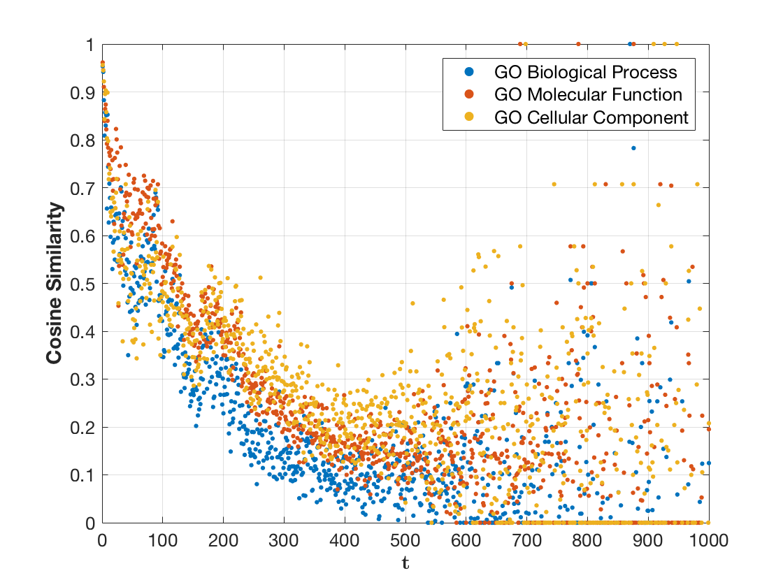
Figure 3: How the similarity of the Gene Ontology annotation vectors between two sequences of a structurally aligned pair in the SCOP2 benchmark varies as a function of the optimal evolutionary distance $n$, under the MMLSUM substitution model.

2.4 Conclusion

A time-dependent substitution matrix and an associated 3-state alignment machine were combined to give a unified statistical model of aligned protein sequences (Section 3 and supplementary Section S1). This model uniquely provides many advantages including the inference of evolutionary distance between two aligned protein sequences (supplementary Section S1.3.3), the estimation of Shannon information content of any benchmark data-set containing a collection of alignments (Section 3.2), and using this to compare between previously published substitution matrices (Section 2.2).

Existing substitution matrices that do not explicitly depend on time were each converted to a corresponding base matrix that can benefit from our information-theoretic framework. Optimal matrices were also inferred using MML for each of six benchmark data-sets of aligned proteins. This allowed us to compare nine existing substitution matrices with the six MML-inferred matrices, on six benchmarks. All MML-inferred matrices perform very well and, in particular, the MMLSUM matrix outperforms all of the other matrices and generalises best of all, across all six benchmarks. The MMLSUM matrix implies sensible groupings of the 20 amino acids (Section 2.3). Increasing evolutionary distance correlates with decreasing similarity of function in aligned proteins, becoming noisy after $t=400$. The complete statistical model yields an interesting relationship between evolutionary distance and the frequency and length of gaps (indels). We have made available the MMLSUM series of log-odds scoring matrices for standard use at https://lcb.infotech.monash.edu.au/mmlsum.

3 Materials and methods

3.1 Introduction to Minimum Message Length framework

The Minimum Message Length (MML) principle [47, 46, 2] is a powerful technique to infer reliable hypotheses (models, theories) from observed data. MML is an information-theoretic criterion that, in its mechanics, combines Bayesian inference [8] with lossless data compression. Formally, the joint probability of any hypothesis $H$ and data $D$ is given by

$$\text{Pr($H,D$)}=\text{Pr($H$)}\text{Pr($D|H$)}=\text{Pr($D$)}\text{Pr($H|D$)}$$

Commonly, model inference depends on identifying suitable hypotheses based on posterior probability (i.e., Pr($H|D$) – the probability of any hypothesis given the data). Separately, Shannon’s Mathematical Theory of Communication [37] quantifies the amount of information in any event $E$ that occurs with a probability of Pr($E$) as:

$$\text{$I(E)$}=-\log_{2}{\text{Pr($E$)}}\quad\text{bits}$$

$I(E)$ can be understood as the minimum lossless encoding length required to communicate the event E. Using this, the joint probability Pr($H,D$) can in turn be expressed in terms of Shannon information content as:

$$\text{$I(H,D)$}=\text{$I(H)$}+\text{$I(D|H)$}=\text{$I(D)$}+\text{$I(H|D)$}$$ (1)

This relationship can be rationalised as the length of a two-part message required to communicate the hypothesis $H$ and the data $D$ given $H$, ($D|H$), as a notional communication between a transmitter and receiver. In this formulation, the transmitter losslessly encodes an hypothesis $H$ which takes $I(H)$ bits to state, followed by the data D given the stated hypothesis H, taking another $I(D|H)$ bits to state. Note, for any $H$ and $D$, $I(H)$ and $I(D|H)$ have to be accurately estimated, and we carry out this estimation using the well-established technique from the statistical-learning literature, due to Wallace and Freeman [48]. Note, one of the important aspects of MML is stating (i.e., lossless encoding) parameter estimates to optimum precision.

Many attractive properties emerge from the MML formulation, but most useful here is the observation that the difference in message lengths between any pair of competing hypotheses (say $H_{1}$ and $H_{2}$) gives the posterior log-odds ratio:

$$\text{$I(H_{1},D)$}-\text{$I(H_{2},D)$} =-\log_{2}{\text{Pr($D$)}\text{Pr($H_{1}|D$)}}+\log_{2}{\text{Pr($D$)}\text{Pr($H_{2}|D$)}}$$

$$=\log_{2}{\left(\frac{\text{Pr($H_{2}|D$)}}{\text{Pr($H_{1}|D$)}}\right)}$$

This allows competing hypotheses to be objectively compared and the best one reliably chosen.

3.2 Formulating the problem in the MML framework

In this work, the observed data $\mathbf{D}$ denotes any data-set of aligned protein sequences. Formally, it is composed of pairs of amino acid sequences and their given alignments:

$$\mathbf{D}=\{\left<\mathcal{A}_{1},S_{1},T_{1}\right>,\left<\mathcal{A}_{2},S_{2},T_{2}\right>,...,\left<\mathcal{A}_{|\mathbf{D}|},S_{|\mathbf{D}|},T_{|\mathbf{D}|}\right>\}$$

where each $S_{i}$ and each $T_{i}$ is a sequence over the alphabet of 20 amino acids, and $\mathcal{A}_{i}$ represents their given alignment relationship specified as a 3-state string over $\{$match, insert, delete$\}$ states. Note that each alignment, $\mathcal{A}_{i}$, is a part of the observed data, coming from structural alignments or from some set of benchmark alignments – see Section 3.3 for details.

A hypothesis $H$ that losslessly explains the above data $\mathbf{D}$ is composed of the following statistical models (and we emphasize all the models shown below are automatically inferred from any given $\mathbf{D}$, as those that are optimal under the MML criterion):

1. A stochastic Markov matrix $\mathbf{M}$ (see Section 3.4) which is used to losslessly encode the corresponding pairs of amino acids in $\left<S_{i},T_{i}\right>$ that are under ‘match’ states in $\mathcal{A}_{i}$. Note, this stochastic matrix can either be optimally inferred under the MML criterion from the collection $\mathbf{D}$ (see Section 3.8), or, for comparison purposes, be any existing substitution matrix (see Section 3.7).

2. A multinomial model, $\mathbf{P}$, of the 20 amino acids, used to losslessly encode the amino acids in the unaligned regions of $\left<S_{i},T_{i}\right>$, i.e., those that are under insert or delete (indel) states in $\mathcal{A}_{i}$. Estimates of $\mathbf{P}$ are optimally inferred using MML from the indel regions observed in alignments in the collection $\mathbf{D}$. (Note, for a comparison, we also explore two other choices for $\mathbf{P}$: one derived from the stationary distribution of $\mathbf{M}$, and the other derived from a source independent of $\mathbf{D}$ (refer supplementary Section S2.2)).

3. A set of automatically inferred Dirichlet parameters $\boldsymbol{\alpha}$ (see Section 3.6), each one specifying a Dirichlet distribution for a specific value of “time”, $t$, to be used in conjunction with $\mathbf{M}(t)$; the alignment 3-state machine’s transition probabilities $\mathbf{\Theta}_{i}$ that is inferred optimally for any alignment $\mathcal{A}_{i}$ are encoded using one of the time-dependent Dirichlet distributions. These transition probabilities in turn are used to losslessly encode a 3-state alignment string $\mathcal{A}_{i}$.

4. Finally, the set of automatically inferred time parameters $\boldsymbol{\tau}=\{t_{1},t_{2},...,t_{N}\}$, one for each sequence-pair in D, using the above models. Each $t_{i}$ captures the divergence of corresponding sequence-pairs $\left<S_{i},T_{i}\right>$, where $t_{i}$ can be interpreted as the length of the Markov chain by which their amino acids are related using the above models.

Using Eq. 1 (see Section 3.1), this framework allows the estimation of the Shannon information content in the hypothesis $H$ and data $\mathbf{D}$ as a summation of individual Shannon information terms:

$$\text{$I(H,\mathbf{D})$}=\text{$I(\mathbf{M})$}+\text{$I(\mathbf{P})$}+\text{$I(\boldsymbol{\alpha})$}+\sum_{i=1}^{|\mathbf{D}|}\text{$I(t_{i})$}+\text{$I(\mathbf{\Theta}_{i}|\boldsymbol{\alpha},t_{i})$}+\text{$I(\mathcal{A}_{i}|\mathbf{\Theta}_{i},t_{i})$}+\text{$I(\left<S_{i},T_{i}\right>|\mathcal{A}_{i},\mathbf{M},\mathbf{P},t_{i})$}$$ (2)

where,
$I(\mathbf{M})$ is the lossless encoding (i.e., statement) length of Matrix $\mathbf{M}$ that models matched parts of $\mathbf{D}$;
$I(\mathbf{P})$ is the statement length of probability estimates $\mathbf{P}$ to model indel parts of $\mathbf{D}$;
$I(\boldsymbol{\alpha})$ is the statement length of inferred time-dependent Dirichlet parameters;
$I(t_{i})$ is the statement length of inferred time $t_{i}$ of a sequence-pair $\left<S_{i},T_{i}\right>$ given its alignment $\mathcal{A}_{i}$;
$I(\mathbf{\Theta}_{i}|\boldsymbol{\alpha},t_{i})$ is the statement length of alignment state machine parameters inferred on each $\mathcal{A}_{i}$;
$I(\mathcal{A}_{i}|\mathbf{\Theta}_{i},t_{i})$ is the statement length of each $\mathcal{A}_{i}$; and
$I(\left<S_{i},T_{i}\right>|\mathcal{A}_{i},\mathbf{M},\mathbf{P},t_{i})$ is the statement length of explaining all amino acids in the sequence-pair.

The models stated above and their MML estimation are briefly described in Sections 3.3–3.9, whereas the full details of their inference are presented in the supplementary Section S1.

3.3 Alignment benchmarks and materials

This work utilises the following benchmarks to validate the framework introduced above. Each benchmark individually provides a source collection $\mathbf{D}$ of pairs of sequences and their given alignment relationships. $\mathbf{D}$ is losslessly compressed under the minimum message length (MML) criterion, Eq. 2.

1. HOMSTRAD [29] (https://mizuguchilab.org/homstrad) is a database of structural alignments for homologous protein families. It contains multiple alignments of proteins covering 1032 families with known structures. Their alignments are semi-manually curated using the structural alignment programs: MNYFIT, STAMP and COMPARER [41, 35, 36].

2. Mattbench [15] (https://bcb.cs.tufts.edu/mattbench/Mattbench.html) curated using the structural alignment program MATT [28]. This work combines into one benchmark, its two sets of alignments classified as superfamily and twilight zone. The superfamily set contains alignments of 225 groups of homologous protein domains, where all pairs of domains in any group have a sequence identity $<50\%$. The twilight zone set is a much smaller and distinct set containing alignments covering 34 distantly related groups, where the sequence identity threshold is $<20\%$ [15].

3. SABMARK [44] (http://bioinformatics.vub.ac.be/databases/databases.html) is a more extensive set of alignments covering superfamily and twilight zone protein domain sets, whose alignments are curated using SOFI and CE [10, 38]. Superfamily set (SABMARK-sup) contains 425 groups of multiple alignments, while the twilight zone set (SABMARK-twi) contains 209 groups.

4. SCOP [5] (https://scop.berkeley.edu) database (v2.07) was used to derive a set of 59,092 unique protein domain pairs, randomly sampled from the superfamily (36,372) and family (22,720) levels of its hierarchy. These 59,092 pairs were aligned separately using DALI [20] and MMLigner [12] to provide SCOP1 and SCOP2 benchmark alignments.

New stochastic models of amino acid exchanges are automatically inferred on the above benchmarks and performance compared to popularly used substitution matrices in Shannon information terms, without the necessity of hand-tuning parameters (as demonstrated in Section 2.2).

3.4 Stochastic matrix $\mathbf{M}$ to model amino acids in the matched regions

Amino acid interchanges are modelled here by a Markov chain [32] defined over the state space of 20 amino acids. The probabilities of transitions between any pairs of amino acid states is represented here as a stochastic matrix $\mathbf{M}$. For any discrete time interval $t>0$, if an amino acid $a_{0}$ (at time $t=0$) undergoes the following chain of interchanges ($a_{0}\rightarrow a_{1}\rightarrow...\rightarrow a_{t-1}\rightarrow a_{t}$), the Markov process ensures that the state of the amino acid $a_{t}$ (at time $t$) depends only on the previous state of the amino acid $a_{t-1}$ (at time $t-1$):

$$\text{Pr($a_{t}|a_{0},a_{1},...,a_{t-1}$)}=\text{Pr($a_{t}|a_{t-1}$)}.$$

Thus, the conditional probability Pr($a_{t}|a_{t-1}$) corresponds to a single step transition between the two states as observed after one discrete unit of time from the time $t-1$.

In this work, $\mathbf{M}$ is represented by a $20\times 20$ matrix containing conditional probabilities, where each cell $\mathbf{M}_{ij}$ gives to the probability of an amino acid indexed by $j$ changing to an amino acid indexed by $i$, in one time-unit (note, $0\leq\mathbf{M}_{ij}\leq 1$ ). Although this time-unit can be arbitrarily defined, it should be small and we use the convention introduced by Dayhoff et al. (1978) [16], and define one time-unit as the time taken for observing a 1% (= 0.01) expected change in amino acids under the model defined by the matrix.

We term the probability matrix $\mathbf{M}$ at time $t=1$, i.e. $\mathbf{M}=\mathbf{M}(1)$, the base matrix. In our formulation, each column vector of $\mathbf{M}$ is an $\mathbb{L}_{1}$ normalised vector (i.e. $\sum_{i=1}^{20}\mathbf{M}_{ij}=1$ for all $1\leq j\leq 20$). Further, as the Markov property holds, $\mathbf{M}(t)$ can be computed from $\mathbf{M}(1)$ as $\mathbf{M}^{t}$, denoting the stochastic matrix after t time-steps. Implicit in $\mathbf{M}$ is its stationary distribution $\pi$ [32] such that $\lim_{t\rightarrow\infty}\mathbf{M}^{t}$ gives a matrix whose columns all tend to $\pi$. This stationary distribution $\pi$ is derived from the eigenvector corresponding to the eigenvalue of $1$ (the largest eigenvalue) of $\mathbf{M}$.

3.5 Multinomial probabilities $\mathbf{P}$ to model the amino acids in the indel region

In general, the multinomial probabilities can be estimated over observations from any finite alphabet $\mathbf{\aleph}=\{x_{1},...,x_{|\mathbf{\aleph}|}\}$ with $|\mathbf{\aleph}|$ symbols/states. The Wallace and Freeman [48] MML-estimate for multinomial probabilities has been derived as (refer [2]):

$$\text{Pr($x_{i}$)}=\frac{n_{i}+\frac{1}{2}}{\sum_{j=1}^{|\mathbf{\aleph}|}n_{j}+\frac{|\mathbf{\aleph}|}{2}}$$

where $n_{i}$ is the number of observations of each state $x_{i}$. Using the above, we derive the optimal MML probability estimates $\mathbf{P}$ of each amino acid by accounting for the number of observations of each amino acid in the indel regions of all alignments in any specified collection $\mathbf{D}$.

To provide an alternate estimate for $\mathbf{P}$, we compare the above optimal choice with those derived from the stationary distribution $\pi$ of the stochastic matrix $\mathbf{M}$. We note that $\pi$ is the eigenvector corresponding to $\mathbf{M}$’s largest eigenvalue whose value is one. Further, both the above candidates for estimates of $\mathbf{P}$ are dependent on the observed data $\mathbf{D}$. To compare these against an estimate independent of $\mathbf{D}$, $\mathbf{P}$ can be estimated on the UniProt database [6] (see supplementary Section S2.2).

3.6 Alignment 3-state machine and Dirichlet distributions as a function of time

In the collection $\mathbf{D}$, any alignment relationship $\mathcal{A}_{i}$ over its corresponding sequences $\left<S_{i},T_{i}\right>$ is described as a 3-state string over the alphabet of {match (m), insert (i), delete (d)} states, as previously considered by Gotoh [18] and Allison et al. [4]. This 3-state machine defines nine possible one-step state transitions, with corresponding transition probabilities (denoted as $\mathbf{\Theta}$) (see Fig. 4), where the sum of probabilities out of any state equals 1. Further, as is common when dealing with alignments of biomolecules, the insert and delete states are treated symmetrically, thus reducing the number of free parameters to three. Notionally these free parameters are represented by $\{\text{Pr($\text{{m}}|\text{{m}}$)},\text{Pr($\text{{i}}|\text{{i}}$)},\text{Pr($\text{{m}}|\text{{i}}$)}\}$. The remaining six (dependent) parameters can be can be derived from these as: $\text{Pr($\text{{i}}|\text{{m}}$)}=\text{Pr($\text{{d}}|\text{{m}}$)}=\frac{1-\text{Pr($\text{{m}}|\text{{m}}$)}}{2}$; $\text{Pr($\text{{d}}|\text{{i}}$)}=\text{Pr($\text{{i}}|\text{{d}}$)}=1-\text{Pr($\text{{i}}|\text{{i}}$)}-\text{Pr($\text{{m}}|\text{{i}}$)}$; $\text{Pr($\text{{d}}|\text{{d}}$)}=\text{Pr($\text{{i}}|\text{{i}}$)}$; $\text{Pr($\text{{m}}|\text{{d}}$)}=\text{Pr($\text{{m}}|\text{{i}}$)}$.

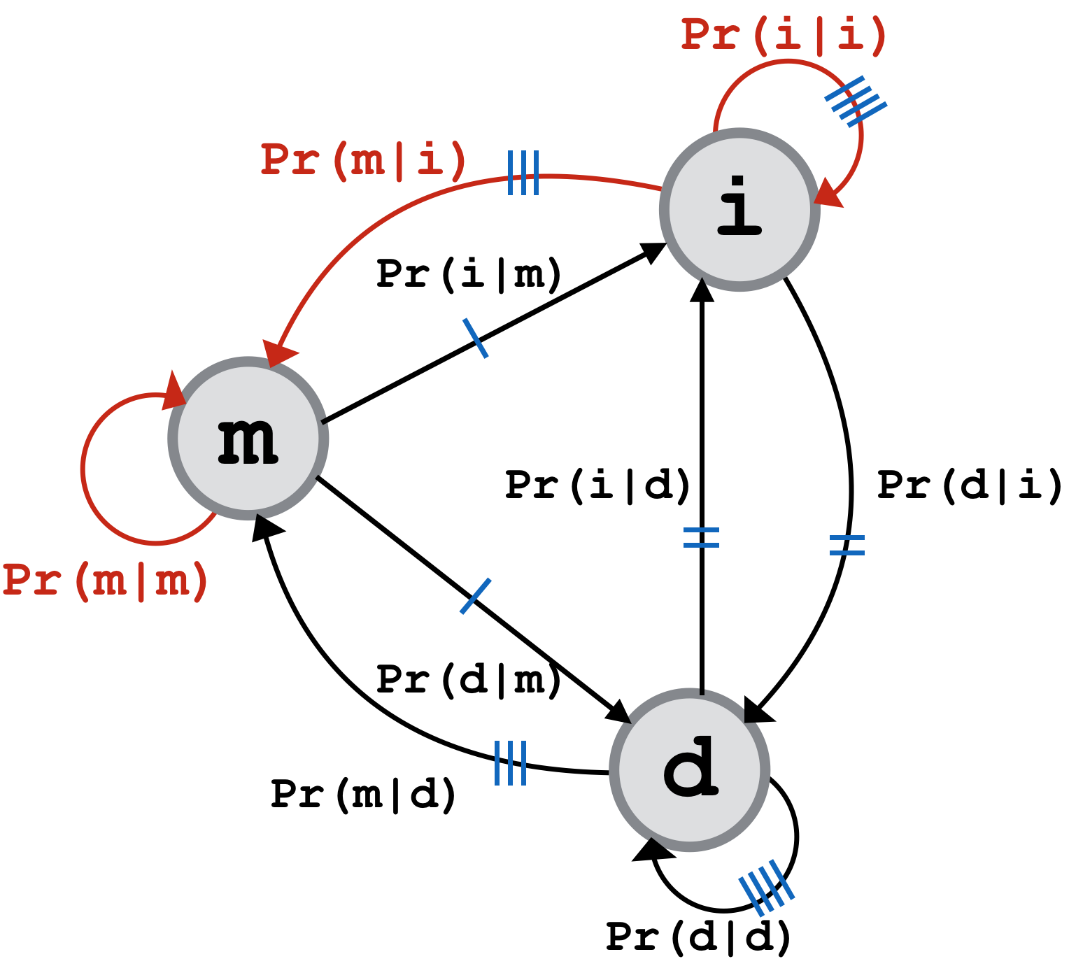
Figure 4: The symmetric 3-state machine for modelling an alignment string (Note: the red colour highlighted transitions refer to the three free parameters. Equivalent transitions are indicated in blue signs)

These 3-state machine parameters are modelled using inferred Dirichlet distributions for different values of time $t$. In general, a Dirichlet distribution is a natural choice to model the parameters of multistate (categorical) and multinomial distributions as the Dirichlet is a conjugate prior of the latter. The time-dependent Dirichlet parameters inferred from $\mathbf{D}$ are denoted as $\boldsymbol{\alpha}(t)$. See supplementary Section S1.3.4 for the methodological details of the inference of time-dependent Dirichlet parameters $\boldsymbol{\alpha}(t)$, and $\mathbf{\Theta}$ given $\boldsymbol{\alpha}(t)$, from any collection of alignments $\mathbf{D}$.

3.7 Converting a substitution scoring matrix to a stochastic matrix $\mathbf{M}$

Any existing substitution matrix can be converted into its corresponding stochastic matrix M and thus benefit from the MML’s unsupervised parameter estimation. This lends the ability to objectively compare the performance of commonly-used scoring matrices over amino acid substitutions. These scoring matrices are normally published in their linearly-scaled log-odds form. These log-odds matrices are converted back to their conditional probability form, by using their reported multiplier and amino acid frequencies. Let $\mathbf{C}$ denote the conditional probability matrix derived from a substitution scoring matrix. Then, $\mathbf{M}$ is derived from $\mathbf{C}$ by numerically identifying the $k$-th root of the matrix $\mathbf{C}$, i.e. $\mathbf{M}(1)=\mathbf{C}^{\frac{1}{k}}$, such that the resulting $\mathbf{M}$ is nearest to 1% (=0.01) expected amino-acid change (refer supplementary Section S1.5.2).

Once the stochastic matrix is derived from an existing substitution scoring matrix, all the other corresponding parameters ($\mathbf{P}$, $\mathbf{\Theta}$, $\boldsymbol{\alpha}$, $\boldsymbol{\tau}$) are automatically inferred, using MML, to be optimal to $\mathbf{M}$ for the given collection $\mathbf{D}$.

3.8 Inference of the best stochastic matrix $\mathbf{M}^{*}$ for any benchmark $\mathbf{D}$

This MML framework also allows the inference of the stochastic matrix from $\mathbf{D}$, the best matrix being the one that minimises the MML objective function given in Eq. 2. To search for the best stochastic matrix over any $\mathbf{D}$, we implement a Monte Carlo search method (see supplementary Section S1.4). Broadly, beginning from an initial state of $\mathbf{M}$, randomly chosen columns of the evolving matrix are perturbed in the near-neighborhood. Using the Metropolis criteria each perturbation is either accepted/rejected over an iterative Monte Carlo process until convergence (refer supplementary Section S1.4).

3.9 Estimation of terms in Eq. 2

The ‘MML87’ method [48] of parameter estimation is used to compute the Shannon information terms in Eq. 2. In general, for a model with continuous parameters $\eta$, and prior $h(\eta)$, Wallace and Freeman (1987) derive the following message length required to explain any observed data-set $d$:

$$\text{$I(\eta,d)$}=\text{$I(\eta)$}+\text{$I(d|\eta)$}$$

where

$$\text{$I(\eta)$}=-\log{[h(\eta)]}+\frac{1}{2}\log{\{det[Fisher(\eta)]\}}+\frac{|\eta|}{2}\log{(\kappa_{|\eta|})}+\frac{|\eta|}{2}$$

($|\eta|$ is the number of free parameters, and $\kappa_{|\eta|}$ is the associated lattice constant [14]).

$$\text{$I(d|\eta)$}=\mathcal{L}(d)$$

$det(Fisher(\eta))$ is the determinant of the Fisher information matrix (the second derivative of the negative log likelihood function) that informs the optimal precision required to state $\eta$. Individual statement lengths of terms in Eq. 2 are described in the supplementary Section S2.

References

- Adami [2004] C. Adami. Information theory in molecular biology. Physics of Life Reviews, 1(1):3–22, 2004.
- Allison [2018] L. Allison. Coding Ockham’s Razor. Springer, 2018. URL https://doi.org/10.1007/978-3-319-76433-7.
- Allison and Yee [1990] L. Allison and C. Yee. Minimum message length encoding and the comparison of macromolecules. Bulletin of Mathematical Biology, 52(3):431–453, 1990.
- Allison et al. [1992] L. Allison, C. Wallace, and C. Yee. Finite-state models in the alignment of macromolecules. Journal of Molecular Evolution, 35(1):77–89, 1992.
- Andreeva et al. [2020] A. Andreeva, E. Kulesha, J. Gough, and A. G. Murzin. The SCOP database in 2020: expanded classification of representative family and superfamily domains of known protein structures. Nucleic Acids Research, 48(D1):D376–D382, 2020.
- Apweiler et al. [2004] R. Apweiler, A. Bairoch, C. H. Wu, W. C. Barker, B. Boeckmann, S. Ferro, E. Gasteiger, H. Huang, R. Lopez, M. Magrane, et al. Uniprot: the universal protein knowledgebase. Nucleic Acids Research, 32(suppl_1):D115–D119, 2004.
- Barton and Sternberg [1987] G. J. Barton and M. J. Sternberg. Evaluation and improvements in the automatic alignment of protein sequences. Protein Engineering, Design and Selection, 1(2):89–94, 1987.
- Bayes [1763] T. Bayes. LII. An essay towards solving a problem in the doctrine of chances. By the late Rev. Mr. Bayes, FRS communicated by Mr. Price, in a letter to John Canton, AMFR S. Philosophical Transactions of the Royal Society of London, 53:370–418, 1763. URL http://www.jstor.org/stable/105741.
- Blake and Cohen [2001] J. D. Blake and F. E. Cohen. Pairwise sequence alignment below the twilight zone. Journal of Molecular Biology, 307(2):721–735, 2001.
- Boutonnet et al. [1995] N. S. Boutonnet, M. J. Rooman, M.-E. Ochagavia, J. Richelle, and S. J. Wodak. Optimal protein structure alignments by multiple linkage clustering: application to distantly related proteins. Protein Engineering, Design and Selection, 8(7):647–662, 1995.
- Chothia and Lesk [1986] C. Chothia and A. M. Lesk. The relation between the divergence of sequence and structure in proteins. The EMBO Journal, 5(4):823, 1986. URL http://www.ncbi.nlm.nih.gov/pmc/articles/PMC1166865/.
- Collier et al. [2017] J. H. Collier, L. Allison, A. M. Lesk, P. J. Stuckey, M. Garcia de la Banda, and A. S. Konagurthu. Statistical inference of protein structural alignments using information and compression. Bioinformatics, 33(7):1005–1013, 2017. URL https://doi.org/10.1093/bioinformatics/btw757.
- Consortium [2004] G. O. Consortium. The Gene Ontology (GO) database and informatics resource. Nucleic Acids Research, 32(suppl_1):D258–D261, 2004.
- Conway and Sloane [1984] J. H. Conway and N. J. Sloane. On the Voronoi regions of certain lattices. SIAM Journal on Algebraic Discrete Methods, 5(3):294–305, 1984.
- Daniels et al. [2011] N. Daniels, A. Kumar, L. Cowen, and M. Menke. Touring protein space with Matt. IEEE/ACM Transactions on Computational Biology and Bioinformatics, 9(1):286–293, 2011.
- Dayhoff et al. [1978] M. Dayhoff, R. Schwartz, and B. Orcutt. 22 a model of evolutionary change in proteins. In Atlas of protein sequence and structure, volume 5, pages 345–352. National Biomedical Research Foundation Silver Spring MD, 1978.
- Do et al. [2005] C. B. Do, M. S. Mahabhashyam, M. Brudno, and S. Batzoglou. Probcons: Probabilistic consistency-based multiple sequence alignment. Genome Research, 15(2):330–340, 2005.
- Gotoh [1982] O. Gotoh. An improved algorithm for matching biological sequences. Journal of Molecular Biology, 162(3):705–708, 1982.
- Henikoff and Henikoff [1992] S. Henikoff and J. G. Henikoff. Amino acid substitution matrices from protein blocks. Proceedings of the National Academy of Sciences, 89(22):10915–10919, 1992.
- Holm and Sander [1993] L. Holm and C. Sander. Protein structure comparison by alignment of distance matrices. Journal of Molecular Biology, 233(1):123–138, 1993.
- Johnson and Overington [1993] M. S. Johnson and J. P. Overington. A structural basis for sequence comparisons: an evaluation of scoring methodologies. Journal of Molecular Biology, 233(4):716–738, 1993.
- Jones et al. [1992] D. T. Jones, W. R. Taylor, and J. M. Thornton. The rapid generation of mutation data matrices from protein sequences. Bioinformatics, 8(3):275–282, 1992.
- Keul et al. [2017] F. Keul, M. Hess, M. Goesele, and K. Hamacher. Pfasum: a substitution matrix from PFAM structural alignments. BMC Bioinformatics, 18(1):293, 2017.
- Le and Gascuel [2008] S. Q. Le and O. Gascuel. An improved general amino acid replacement matrix. Molecular Biology and Evolution, 25(7):1307–1320, 2008.
- Lefranc et al. [2015] M.-P. Lefranc, V. Giudicelli, P. Duroux, J. Jabado-Michaloud, G. Folch, S. Aouinti, E. Carillon, H. Duvergey, A. Houles, T. Paysan-Lafosse, et al. IMGT, the international ImMunoGeneTics information system 25 years on. Nucleic Acids Research, 43(D1):D413–D422, 2015.
- Lesk [2016] A. M. Lesk. Introduction to Protein Science: Architecture, Function, and Genomics. Oxford University Press, 2016.
- Löytynoja and Goldman [2008] A. Löytynoja and N. Goldman. Phylogeny-aware gap placement prevents errors in sequence alignment and evolutionary analysis. Science, 320(5883):1632–1635, 2008.
- Menke et al. [2008] M. Menke, B. Berger, and L. Cowen. Matt: local flexibility aids protein multiple structure alignment. PLoS Computational Biology, 4(1):e10, 2008.
- Mizuguchi et al. [1998] K. Mizuguchi, C. Deane, T. Blundell, and J. Overington. HOMSTRAD: a database of protein structure alignments for homologous families. Protein Science, 7(11):2469–2471, 1998.
- Müller et al. [2002] T. Müller, R. Spang, and M. Vingron. Estimating amino acid substitution models: a comparison of Dayhoff’s estimator, the resolvent approach and a maximum likelihood method. Molecular Biology and Evolution, 19(1):8–13, 2002.
- Murzin et al. [1995] A. G. Murzin, S. E. Brenner, T. Hubbard, and C. Chothia. SCOP: a structural classification of proteins database for the investigation of sequences and structures. Journal of Molecular Biology, 247(4):536–540, 1995.
- Norris and Norris [1998] J. R. Norris and J. R. Norris. Markov chains, volume 2. Cambridge university press, 1998.
- Platzer [2013] A. Platzer. Visualization of SNPs with t-SNE. PloS One, 8(2):e56883, 2013.
- Rost [1999] B. Rost. Twilight zone of protein sequence alignments. Protein Engineering, 12(2):85–94, 1999.
- Russell and Barton [1992] R. B. Russell and G. J. Barton. Multiple protein sequence alignment from tertiary structure comparison: assignment of global and residue confidence levels. Proteins: Structure, Function, and Bioinformatics, 14(2):309–323, 1992.
- Sali and Blundell [1990] A. Sali and T. Blundell. The definition of topological equivalence in homologous and analogous structures: A procedure involving comparison of local properties and structural relationships through dynamic programming and simulated annealing. Journal of Molecular Biology, 212:403–428, 1990.
- Shannon [1948] C. E. Shannon. A mathematical theory of communication. Bell System Technical Journal, 27:379–423, 1948.
- Shindyalov and Bourne [1998] I. N. Shindyalov and P. E. Bourne. Protein structure alignment by incremental combinatorial extension (CE) of the optimal path. Protein Engineering, 11(9):739–747, 1998.
- Strait and Dewey [1996] B. J. Strait and T. G. Dewey. The Shannon information entropy of protein sequences. Biophysical Journal, 71(1):148–155, 1996.
- Sumanaweera et al. [2019] D. Sumanaweera, L. Allison, and A. S. Konagurthu. Statistical compression of protein sequences and inference of marginal probability landscapes over competing alignments using finite state models and dirichlet priors. Bioinformatics, 35(14):i360–i369, 2019.
- Sutcliffe et al. [1987] M. J. Sutcliffe, I. Haneef, D. Carney, and T. Blundell. Knowledge based modelling of homologous proteins, Part I: Three-dimensional frameworks derived from the simultaneous superposition of multiple structures. Protein Engineering, Design and Selection, 1(5):377–384, 1987.
- Swanson [1984] R. Swanson. A unifying concept for the amino acid code. Bulletin of Mathematical Biology, 46(2):187–203, 1984.
- van der Maaten and Hinton [2008] L. van der Maaten and G. Hinton. Visualizing data using t-SNE. Journal of Machine Learning Research, 9(Nov):2579–2605, 2008.
- Van Walle et al. [2005] I. Van Walle, I. Lasters, and L. Wyns. SABmark—a benchmark for sequence alignment that covers the entire known fold space. Bioinformatics, 21(7):1267–1268, 2005.
- Vingron and Waterman [1994] M. Vingron and M. S. Waterman. Sequence alignment and penalty choice: Review of concepts, case studies and implications. Journal of Molecular Biology, 235(1):1–12, 1994.
- Wallace [2005] C. S. Wallace. Statistical and inductive inference by minimum message length. Science & Business Media. Springer, 2005. URL https://doi.org/10.1007/0-387-27656-4.
- Wallace and Boulton [1968] C. S. Wallace and D. M. Boulton. An information measure for classification. The Computer Journal, 11(2):185–194, 1968.
- Wallace and Freeman [1987] C. S. Wallace and P. R. Freeman. Estimation and inference by compact coding. Journal of the Royal Statistical Society. Series B (Methodological), pages 240–265, 1987. URL http://www.jstor.org/stable/2985992.
- Whelan and Goldman [2001] S. Whelan and N. Goldman. A general empirical model of protein evolution derived from multiple protein families using a maximum-likelihood approach. Molecular Biology and Evolution, 18(5):691–699, 2001.
- Yamada and Tomii [2013] K. Yamada and K. Tomii. Revisiting amino acid substitution matrices for identifying distantly related proteins. Bioinformatics, 30(3):317–325, 2013.