Multivariate Estimations of Equilibrium Climate Sensitivity from Short Transient Warming Simulations

Abstract

One of the most used metrics to gauge the effects of climate change is the equilibrium climate sensitivity, defined as the long-term (equilibrium) temperature increase resulting from instantaneous doubling of atmospheric CO₂. Since global climate models cannot be fully equilibrated in practice, extrapolation techniques are used to estimate the equilibrium state from transient warming simulations. Because of the abundance of climate feedbacks – spanning a wide range of temporal scales – it is hard to extract long-term behaviour from short-time series; predominantly used techniques are only capable of detecting the single most dominant eigenmode, thus hampering their ability to give accurate long-term estimates. Here, we present an extension to those methods by incorporating data from multiple observables in a multi-component linear regression model. This way, not only the dominant but also the next-dominant eigenmodes of the climate system are captured, leading to better long-term estimates from short, non-equilibrated time series.

1 Introduction

The use of (equilibrium) climate sensitivity to assess the impact of changes in atmospheric CO₂ dates back at least a century Arrhenius (1896); Lapenis (1998). First, estimations of its value were made with rudimentary computations Arrhenius (1896); Charney . (1979); nowadays, improved knowledge of the climate system is used to infer climate sensitivity from observational data, proxy data, and global climate models Knutti  Hegerl (2008); Von der Heydt . (2016); Rohling . (2018); Lunt . (2010); Knutti . (2017). However, the reported values (still) vary much between studies IPCC (2013) and the current consensus is that climate sensitivity is between $2.3K$ and $4.7K$ <5%-95% ranges,¿Sherwood2020. On top of that, recent results of the new generation of global climate models show even higher sensitivities, possibly due to better representation of cloud formation when using finer spatial grids Bacmeister . (2020); Zelinka . (2020); Andrews . (2019); Bony . (2015); Duffy . (2003); Govindasamy . (2003); Haarsma . (2016). Still, even these state-of-the-art climate models report significantly different climate sensitivities Flynn  Mauritsen (2020); Zelinka . (2020); Forster . (2020); moreover, estimates for a single model tend to have large uncertainties further hampering accurate pinpointing of the climate sensitivity Rugenstein . (2020); Dai . (2020).

For conceptual models and earth system models of intermediate complexity, it is possible to let a simulation run until the system is fully equilibrated Holden . (2014). However, for more refined models, including contemporary and future state-of-the-art global climate models, this is not viable Rugenstein . (2019); equilibrating those models simply takes too much computing power. With the current trend – and need – to build models with higher temporal and spatial resolutions Eyring . (2016); Duffy . (2003); Govindasamy . (2003); Haarsma . (2016), this is not expected to resolve itself in the near future. Hence, the equilibrium climate sensitivity of these models is instead estimated by extrapolating transient warming simulations – way before these models have reached equilibrium Knutti  Hegerl (2008); Rugenstein . (2020); Dai . (2020); Knutti . (2017). There are several techniques to perform such extrapolation that use different physical and mathematical properties of the system to give sensible estimates for the true equilibrium climate sensitivity of a model Knutti  Hegerl (2008); Dai . (2020); Gregory . (2004); Geoffroy, Saint-Martin, Bellon . (2013); Proistosescu  Huybers (2017).

The main problem with equilibrium estimations lies with the abundance of feedbacks present in the climate system Von der Heydt . (2016, 2020). These feedbacks are quite diverse and span a wide range of spatial and temporal scales; these include, for example, the very fast Planck feedback, the slower ice-albedo feedback and the even slower ocean circulation feedbacks. Estimation techniques deal differently with this problem, for instance by incorporating multiple time scales directly in the estimation method Proistosescu  Huybers (2017), by explicit modelling of long-term (ocean) heat uptake Geoffroy, Saint-Martin, Bellon . (2013) or more indirectly by ignoring initial fast warming behaviour Rugenstein . (2020); Dai . (2020).

The most predominantly used estimation technique is the one developed by gregory2004new. In this technique, the top-of-atmosphere radiative imbalance ($\Delta R$) is fitted using a linear regression against the temperature increase ($\Delta T$). However, recently, it has become clear that $\Delta R$ and $\Delta T$ do not always adhere to such linear relationship Andrews . (2012); Armour (2017); Knutti  Rugenstein (2015). Typically, there is an initial fast warming which is followed by one or several slower additional (less substantial) warming processes. Hence, estimates made by this method depend heavily on the time period used in the regression and typically underestimate the equilibrium warming. Most of the times, this problem is largely circumvented by ignoring the first part of a simulation that contains the initial fast processes; the regression is then applied only on the last part of the simulation.

The thus ignored data does however still contain information about the dynamics of the system – even beyond the initial fast warming. The issue here is that this information cannot be extracted using a one-dimensional linear regression; that kind of fit will only ever recover the one process (i.e. one eigenmode of decay to equilibrium) that is most dominantly present on the time scale of the regression data. In this paper, we present an extension to this technique that is capable of capturing multiple eigenmodes by incorporating additional observables into a multi-component linear regression (abbreviated as MC-LR) model. Subsequently, we show the potential efficiency of this technique using both low dimensional conceptual models and modern global climate models.

2 Method: a Multi-Component Linear Regression Model

In the linear regime of the decay to equilibrium, the evolution of any observable $O$ (e.g. global mean temperature increase or top-of-atmosphere radiative imbalance) is given by the sum of exponentials (i.e. the eigenvalue decomposition), capturing the behaviour on different time scales based on the different eigenmodes of the system. Specifically, denoting the equilibrium value of an observable by $O_{*}$, this evolution follows

$$O(t)-O_{*}=\sum_{j}\beta^{[O]}_{j}e^{\lambda_{j}t},\hskip 56.9055pt\left(\sum_{j}\beta^{[O]}_{j}=O(0)-O_{*}\right)$$ (1)

where $\lambda_{j}$ denote the eigenvalues and $\beta^{[O]}_{j}$ the contributions of each eigenmode to the evolution of the observable $O$.

If only one eigenmode would be present (or relevant, as other eigenmodes are exponentially small on the time scale of the data), the evolution of the global mean surface temperature increase $\Delta T$ and the top-of-atmosphere radiative imbalance $\Delta R$ can be combined into the linear relation

$$\Delta R-\Delta R_{*}=\frac{\beta^{[\Delta R]}_{1}}{\beta^{[\Delta T]}_{1}}\left(\Delta T-\Delta T_{*}\right).$$ (2)

Since $\Delta R_{*}=0$, this readily gives rise to the commonly used regression model by gregory2004new,

$$\Delta R=a\Delta T+f$$ (3)

where $a:=\frac{\beta_{1}^{[\Delta R]}}{\beta_{1}^{[\Delta T]}}$ and $f:=-a\Delta T_{*}$ are to be determined from the used regression data. In this case, the equilibrium warming is estimated by $\Delta T_{*}^{\mathrm{est}}:=-\frac{1}{a}f$.

If multiple eigenmodes are relevant, there no longer is such linear relationship between $\Delta R$ and $\Delta T$ (as time $t$ cannot be eliminated from the equations anymore) and this technique breaks down. It is, however, possible to extend the technique by taking additional observables into account: if $N$ eigenmodes are relevant, one must use two sets of $N$ observables, denoted here by $\vec{X}$ and $\vec{Y}$; using a similar procedure, the equations for their evolutions can be combined together (e.g. using basic matrix computations) to obtain the linear relation

$$\vec{Y}-\vec{Y}_{*}=A\left(\vec{X}-\vec{X}_{*}\right),$$ (4)

where $A$ is a $N\times N$ matrix. If the set of observables in $\vec{Y}$ only contains observables that tend to zero in equilibrium (i.e. $Y_{*}=0$), this gives rise to a new multi-component linear regression model

$$\vec{Y}=A\vec{X}+\vec{F},$$ (5)

with $A$ and $\vec{F}:=-A\vec{X}_{*}$ to be determined by the regression data. Here, equilibrium estimates are given by the vector $\vec{X}_{*}^{\mathrm{est}}:=-A^{-1}\vec{F}$ and contain equilibrium estimates for all observables in $\vec{X}$.

The method by gregory2004new is a special example of this regression model, where $N=1$, $\vec{X}=\Delta T$ and $\vec{Y}=\Delta R$. Here, this model is extended by adding one or two observables to the data vectors $\vec{X}$ and $\vec{Y}$ (i.e. $N=2$ or $N=3$, lining up with previous studies by caldeira2013projections, tsutsui2017quantification, proistosescu2017slow). Specifically, the mean global effective top-of-atmosphere short-wave albedo $\alpha$ and long-wave emissivity $\varepsilon$ are considered as additional observables. Their values are added to the data vector $\vec{X}$ and the values of their (numerical) time-derivatives – that tend to zero in equilibrium – to $\vec{Y}$. The fits in this study are all made using standard least squares regression.

A different and much more extensive take on the rationale behind the technique can be found in Supporting Information Text S1.

3 Results: Conceptual Models

First, we present the results on a variant of the conceptual Budyko-Sellers energy balance model for global mean surface temperature Budyko (1969); Sellers (1969). This model has been extended such that albedo and emissivity are no longer instantaneous processes, but will settle slowly over time. Moreover, white noise has been added to simulate climate variability. Thus, a three-component stochastic ordinary differential equation is created, which has been simulated in MATLAB with an Euler-Maruyama scheme. A more extensive description of the model can be found in Supporting Information Text S2.

Output of this model has been analyzed using the previously described MC-LR technique with the use of some or all of the observables. The resulting estimates for the equilibrium climate increase $\Delta T^{\mathrm{est}}_{*}(t)$ are given in Figure 1 for simulation runs with moderate noise (figures for other noise levels can be found in Supporting Information Figures S3 and S4). These estimates are given as functions of model time: the value for time $t$ indicates the estimate is made with model output up to time $t$ only. To evaluate the various estimation techniques and track their accuracy depending on the amount of data used, the remaining relative error is computed: the maximum in relative error of the estimates occurring after the current time (i.e. when more data points are used). This gives a better impression of the kind of error to expect when using data up to time $t$. Mathematically, the remaining error is defined as

$$e_{\mathrm{rem}}^{\mathrm{rel}}(t):=\max_{s\geq t}\left|\frac{\Delta T_{*}^{\mathrm{est}}(s)-\Delta T_{*}}{\Delta T_{*}^{\mathrm{est}}(s)}\right|,$$ (6)

where $\Delta T_{*}$ is the true equilibrium warming (determined numerically via Newton’s method).

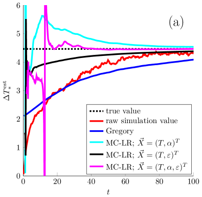
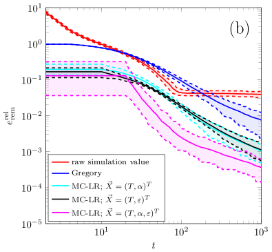
Figure 1: Results from various estimation techniques on a conceptual ($3$-component) global energy budget model with moderate noise (noise strength $\nu=0.5$ – see Supporting Information Text S2 for details). (a) Estimates $\Delta T_{*}^{\mathrm{est}}(t)$ for a single model realisation; the value at time $t$ gives the estimation when only data up to time $t$ is used. (b) Evolution of expected remaining error $e_{\mathrm{rem}}^{\mathrm{rel}}(t)$ over time based on an ensemble of one hundred runs; solid lines indicate mean values and dashed lines the $5$ and $95$ percentile values. Results on models with different noise levels can be found in Supporting Information Figures S3 and S4.

For this kind of low-dimensional models, it is clear that the multi-component linear regression leads to better estimations of the real equilibrium warming than conventional techniques (Figure 1). Although the estimations for very short time series are not very accurate, estimations for slightly longer time series quickly pick up and are much better compared to the linear ‘Gregory’ fit (Figure 1a), because also the longer time dynamics are taken into account (and are accurately fitted; see Supporting Information Text S2 and Figure S5). It takes some tens of (arbitrary) time units for the new estimates to get within $0.1K$ of the actual equilibrium value, whereas hundreds of time units are needed for the conventional technique (Figure 1b). Moreover, it also seems that the MC-LR technique still works reliable in case of noise.

4 Results: LongRunMIP Models

The MC-LR technique has also been tested on more detailed global climate models. Specifically, data is taken from abrupt $4\times\mathrm{CO}_{2}$ forcing experiments of models participating in LongRunMIP, a model intercomparison project that focuses on millennia-long simulation runs Rugenstein . (2019). Because of these long time series, a relative accurate value for the true equilibrium temperature can be determined, which is needed to adequately assess the performance of the estimation techniques.

For these climate models, global data on near-surface atmospheric temperature ($T$ = ‘tas’) and top-of-atmosphere radiative fluxes (incoming short-wave, ‘rsdt’, outgoing short-wave, ‘rsut’ and outgoing long-wave, ‘rlut’) has been downloaded from the LongRunMIP data server Rugenstein . (2019). These datasets have been used to compute top-of-atmosphere radiative imbalance ($R$ = ‘rsdt’ - ‘rsut’ - ‘rlut’), effective short-wave albedo ($\alpha$ = ‘rsut’ / ‘rsdt’) and effective long-wave emissivity ($\varepsilon\sigma$ = ‘rlut’ / (‘tas’)⁴; where $\sigma$ is the Stefan–Boltzmann constant). Initial, non-forced values were defined as means of piControl runs and changes $\Delta T$, $\Delta R$, $\Delta\alpha$ and $\Delta\varepsilon\sigma$ were computed from the abrupt $4\times$CO₂ forcing runs. The real equilibrium warming $\Delta T_{*}$ for these models was estimated from the last warming of the forcing experiments, following the approach taken in Rugenstein2020. A more detailed description of these procedures, including minor practical variants, can be found in Supporting Information Text S3.

With the use of the model output, various techniques have been used to estimate equilibrium warming for all models. In Figure 2, a Gregory $(\Delta T,\Delta R)$-plot is given along with results of commonly used estimation techniques for one of the models (CESM 1.0.4) when applied on data up to model year $300$. This illustrates the capabilities of the various techniques in capturing the behaviour of the model system over different time scales. Clearly, the classical Gregory method mainly captures initial fast warming from the data. Hence, it is common practice to ignore an arbitrary number of years from the start of the simulation run – that show the initial fast warming – in a Gregory fit Rugenstein . (2020); Dai . (2020). That technique has also been tested here, where the initial $20$ years have been excluded. In contrast, the multi-component linear regression technique does not rely on such arbitrary choices for data selection and outperforms both of these classical methods. Certainly, there also exist other alternative estimation techniques that aim to extract long-term behaviour from short simulation runs (of which two have been added to Figure 2). However, these often amount to fitting an explicit low-dimensional model to transient simulations <e.g.¿geoffroy2013transient and/or a non-linear regression <e.g.¿proistosescu2017slow. The proposed MC-LR method does neither – and furthermore seems to perform similar or better than the mentioned other methods.

The results for other time frames are shown in Figure 3. Here, as before, estimates $\Delta T_{*}^{\mathrm{est}}(t)$ are functions of time, which only use data up to a given time $t$ for the estimation, and remaining relative errors have been computed as well. These results show that the MC-LR method also performs better on other time frames; in particular, when data for more than 150 years is being used, a multi-component linear regression that utilises both albedo and emissivity leads to better estimates compared to the classical Gregory methods. Especially on a century time scale this leads to significant improvements. Detailed results for all models can be found in Supporting Informaiton Figures S8-S18.

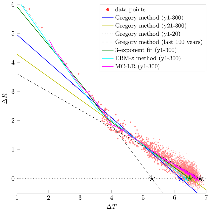
Figure 2: Gregory plot of $\Delta R$ as function of $\Delta T$ for a $5,900$ year abrupt CO₂ quadrupling experiment in the CESM 1.0.4 model along with results of various common equilibrium estimation methods and the here introduced multi-component linear regression (MC-LR) method when used on data up to model year $300$. In the plot, red dots denote all data points (the later in the run, the smaller in size). The blue line shows the linear ‘Gregory’ fit when all data from years $1$ to $300$ is used and the yellow line the Gregory fit when the first $20$ years are ignored. The green line shows the $3$ exponent fit Proistosescu  Huybers (2017). The cyan line indicates a fit to the EBM-$\varepsilon$ model that includes ocean heat uptake Geoffroy, Saint-Martin, Bellon . (2013). The magenta line visualises the newly introduced multi-component linear regression that, in this case, utilises both albedo and emissivity (for this visualisation only – and not for any of the fits in this paper – averaged data from the experiment are used). The stars ($\star$) are the estimated equilibrium warming values from the different methods. Finally, dotted and dashed black lines indicate linear Gregory fits for the first and last part of the simulation that can be used for comparison – and that show how the various estimation methods capture dynamics on multiple time scales.

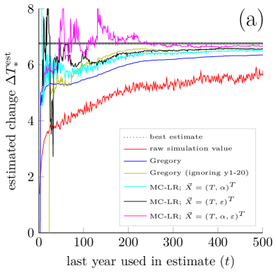
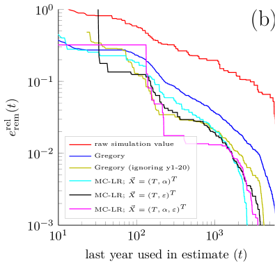
Figure 3: Performance of equilibrium warming estimation techniques on the model CESM 1.0.4. (a) Estimated equilibrium temperature increase $\Delta T_{*}^{\mathrm{est}}(t)$ for various estimators as function of time $t$, where only model output data up to time $t$ has been used. The shaded region indicates the range of likely values for the system’s true equilibrium warming $\Delta T_{*}$, along with the best estimate for this (dashed line), based on end-of-simulation data (see the Supporting Information Text S3.4). Only the first 500 years of the 5900 year simulation are shown. (b) Plot of the remaining relative error for estimation methods based on the whole simulation run. This shows the kind of error to expect when using a certain estimation technique on a given time scale. Full set of results for this and the other models can be found in Supporting Information Figures S8-S18.

To further disseminate the results and to assess the effectiveness over the range of models, in Figure 4 the remaining errors are given for all considered models at given times $t=150$ years (CMIP protocol, eyring2016overview), $t=300$ years and $t=500$ years. These results indicate that the MC-LR method can lead to more accurate equilibrium warming estimates. This new approach also better captures the long-term dynamics than the classical Gregory method when used on all data (with the HadGEM2 model for $t=150$ years being the exception, where performance is similar). Moreover, the MC-LR method also tends to outperform the Gregory method that ignores the first $20$ years of data when $t>150$ years. For $t=150$ years, results vary much per model. This is closely related to the difference in model behaviour: if dynamics happen on two dominant time scales, and the Gregory plot has an inflection point around (the arbitrarily chosen) year $20$, this Gregory method works well (see for example the model MPI-ESM 1.1); otherwise, the MC-LR method will (eventually) outperform it. A more in-depth discussion per model is included in Supporting Information Text S3.5.

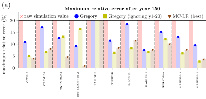
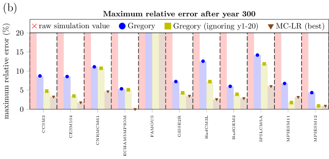
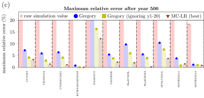
Figure 4: Remaining relative error for various estimation techniques when used on model output up to (a) $t=150y$, (b) $t=300y$ and (c) $t=500y$. Here, only the best MC-LR method is depicted for each model (because of differences in model dynamics, which observables yield the best estimates differs per model). A complete list for all variants of the estimation techniques can be found in Supporting Information Figure S6, and a scatter plot of the results in this figure can be found in Supporting Information Figure S5.

5 Discussion

In this paper, we have introduced a new equilibrium climate sensitivity estimation technique – the multi-component linear regression (MC-LR) – that better captures the long-term behaviour compared to conventional techniques. This MC-LR method has one prime rationale: a perturbed climate system evolves according to a linear system (given that the radiative perturbation is small). This linear evolution is recovered through the multi-component linear regression (i.e. regression to $\vec{Y}=A\vec{X}+\vec{F}$). Although, here, only data from one transient simulation is used in the fits, data from multiple runs (with the same radiative forcing) can also be put together – possibly leading to even better estimates. As the goal of the method is to recover the eigenmodes in the linear regime of the system, such combination of runs seems extremely beneficial if runs follow the evolution of different eigenmodes. Indeed, it seems plausible – and an interesting direction for further research – that a small ensemble of short runs, each with a different perturbation of the initial system state, will better estimate the coefficients of the fitted linear system (i.e. $A$ and $\vec{F}$) without compromising in terms of total computing power.

The most difficult – and the most important – aspect of the MC-LR method is the choice of the observables used in the regression data. It is key that this data well-represents the different eigenmodes of the system. If too few are used, not all eigenmodes are found; if too many (or redundant ones) are used, estimates become unusable (as data becomes linearly dependent, which causes the fitted matrix $A$ to become near singular). In this study, we have focused on the use of (effective top-of-atmosphere) albedo and/or emissivity – observables that can be computed from datasets that are already normally used for climate sensitivity Gregory . (2004); Geoffroy, Saint-Martin, Bellon . (2013); Proistosescu  Huybers (2017). However, the use of other, more curated observables might – and probably will – work better. For instance, the very long-term ocean dynamics might be better represented in data on ocean heat uptake Geoffroy, Saint-Martin, Bellon . (2013); Geoffroy, Saint-Martin, Olivié . (2013); Raper . (2002); Li . (2013). It also seems natural to capture the known climate feedbacks, e.g. surface albedo, water vapour and lapse rate Von der Heydt . (2020). One should beware though that all these (feedback) processes together combine to the system’s eigenmodes in non-straightforward ways. For example, summing feedbacks – like is commonly done in climate literature – only makes sense in systems that only have one component; in systems with multiple components, processes and eigenmodes are not linked directly like this. Nevertheless, a careful inclusion of these feedbacks might lead to even better estimates and may further shorten the needed length of simulation runs.

The method described in this study does not only lead to better estimates for the equilibrium climate sensitivity, but can also be used to develop extensions of climate sensitivity, by incorporating other observables. Regression of the multi-component model $\vec{Y}=A\vec{X}+\vec{F}$ leads to equilibrium estimates for all the observables in $\vec{X}$ as $\vec{X}_{*}^{\mathrm{est}}=-A^{-1}\vec{F}$. This estimate can be seen as a multi-variate metric for climate sensitivity, in contrast to classical uni-variate metrics that focus only on changes in global temperature. Such multivariate metrics can better describe and quantify the changes that occur to the climate system due to changes in radiative forcing. In fact, many – if not all – climate subsystems and ecosystems do not depend critically on the global mean surface temperature, but on other observables such as the amount of precipitation or ocean heat transport Lenton . (2008); Scheffer . (2009); Rockström . (2009). Estimating those directly – rather than considering them enslaved to the global mean surface temperature – will possibly lead to better projections for those (sub)systems.

Accurate estimations of equilibrium climate sensitivity are hard to come by, mostly due to the lengthy computation times needed to fully equilibrate modern global climate models. Going forward, it seems the more and more realistic state-of-the-art models will only take longer and longer to equilibrate (even considering developments in computer hardware). In particular, for high-resolution simulations with ultra fine numerical grids such equilibration runs are just not a practical option. For these kind of simulations it is vital to have extrapolation techniques that only need relatively short transient simulations to estimate the system’s long-term behaviour. Once fully developed, such methods – the one introduced in this study being a first step towards them – can help to design the kind, amount and length of the experiments performed with these high-resolution models, indicating an optimum between accurate (multi-variate) climate sensitivity estimation and computing time.

References

- Andrews \BOthers. (\APACyear2019) \APACinsertmetastarAndrews2019{APACrefauthors}Andrews, T., Andrews, M\BPBIB., Bodas-Salcedo, A., Jones, G\BPBIS., Kuhlbrodt, T., Manners, J.\BDBLTang, Y. \APACrefYearMonthDay2019. \BBOQ\APACrefatitleForcings, feedbacks, and climate sensitivity in HadGEM3-GC3.1 and UKESM1 Forcings, feedbacks, and climate sensitivity in HadGEM3-GC3.1 and UKESM1.\BBCQ \APACjournalVolNumPagesJournal of Advances in Modeling Earth Systems11124377–4394. {APACrefDOI} \doi10.1029/2019MS001866 \PrintBackRefs\CurrentBib
- Andrews \BOthers. (\APACyear2012) \APACinsertmetastarAndrews2012{APACrefauthors}Andrews, T., Gregory, J\BPBIM., Webb, M\BPBIJ.\BCBL \BBA Taylor, K\BPBIE. \APACrefYearMonthDay2012. \BBOQ\APACrefatitleForcing, feedbacks and climate sensitivity in CMIP5 coupled atmosphere-ocean climate models Forcing, feedbacks and climate sensitivity in CMIP5 coupled atmosphere-ocean climate models.\BBCQ \APACjournalVolNumPagesGeophysical Research Letters3991–7. {APACrefDOI} \doi10.1029/2012GL051607 \PrintBackRefs\CurrentBib
- Armour (\APACyear2017) \APACinsertmetastararmour2017energy{APACrefauthors}Armour, K\BPBIC. \APACrefYearMonthDay2017. \BBOQ\APACrefatitleEnergy budget constraints on climate sensitivity in light of inconstant climate feedbacks Energy budget constraints on climate sensitivity in light of inconstant climate feedbacks.\BBCQ \APACjournalVolNumPagesNature Climate Change75331–335. {APACrefDOI} \doi10.1038/nclimate3278 \PrintBackRefs\CurrentBib
- Arrhenius (\APACyear1896) \APACinsertmetastarArrhenius1896{APACrefauthors}Arrhenius, S. \APACrefYearMonthDay1896. \BBOQ\APACrefatitleOn the influence of carbonic acid in the air upon the temperature of the ground On the influence of carbonic acid in the air upon the temperature of the ground.\BBCQ \APACjournalVolNumPagesThe London, Edinburgh, and Dublin Philosophical Magazine and Journal of Science41251237–276. {APACrefDOI} \doi10.1086/121158 \PrintBackRefs\CurrentBib
- Bacmeister \BOthers. (\APACyear2020) \APACinsertmetastarBacmeister2020{APACrefauthors}Bacmeister, J\BPBIT., Hannay, C., Medeiros, B., Gettelman, A., Neale, R., Fredriksen, H\BHBIB.\BDBLOtto-Bliesner, B\BPBIL. \APACrefYearMonthDay2020. \BBOQ\APACrefatitleCO2 increase experiments using the Community Earth System Model (CESM): Relationship to climate sensitivity and comparison of CESM1 to CESM2 CO2 increase experiments using the community earth system model (CESM): Relationship to climate sensitivity and comparison of CESM1 to CESM2.\BBCQ \APACjournalVolNumPagesEarth and Space Science Open Archive47. {APACrefDOI} \doi10.1002/essoar.10502611.1 \PrintBackRefs\CurrentBib
- Bony \BOthers. (\APACyear2015) \APACinsertmetastarbony2015clouds{APACrefauthors}Bony, S., Stevens, B., Frierson, D\BPBIM., Jakob, C., Kageyama, M., Pincus, R.\BDBLWebb, M\BPBIJ. \APACrefYearMonthDay2015. \BBOQ\APACrefatitleClouds, circulation and climate sensitivity Clouds, circulation and climate sensitivity.\BBCQ \APACjournalVolNumPagesNature Geoscience84261–268. {APACrefDOI} \doi10.1038/ngeo2398 \PrintBackRefs\CurrentBib
- Budyko (\APACyear1969) \APACinsertmetastarbudyko1969effect{APACrefauthors}Budyko, M\BPBII. \APACrefYearMonthDay1969. \BBOQ\APACrefatitleThe effect of solar radiation variations on the climate of the Earth The effect of solar radiation variations on the climate of the earth.\BBCQ \APACjournalVolNumPagesTellus215611–619. {APACrefDOI} \doi10.3402/tellusa.v21i5.10109 \PrintBackRefs\CurrentBib
- Caldeira \BBA Myhrvold (\APACyear2013) \APACinsertmetastarcaldeira2013projections{APACrefauthors}Caldeira, K.\BCBT \BBA Myhrvold, N. \APACrefYearMonthDay2013. \BBOQ\APACrefatitleProjections of the pace of warming following an abrupt increase in atmospheric carbon dioxide concentration Projections of the pace of warming following an abrupt increase in atmospheric carbon dioxide concentration.\BBCQ \APACjournalVolNumPagesEnvironmental Research Letters83034039. {APACrefDOI} \doi10.1088/1748-9326/8/3/034039 \PrintBackRefs\CurrentBib
- Charney \BOthers. (\APACyear1979) \APACinsertmetastarCharney1979{APACrefauthors}Charney, J\BPBIG., Arakawa, A., Baker, D\BPBIJ., Bolin, B., Dickinson, R\BPBIE., Goody, R\BPBIM.\BDBLWunsch, C\BPBII. \APACrefYear1979. \APACrefbtitleCarbon dioxide and climate: A scientific assessment Carbon dioxide and climate: A scientific assessment. \APACaddressPublisherWashington, DCThe National Academies Press. {APACrefDOI} \doi10.17226/12181 \PrintBackRefs\CurrentBib
- Dai \BOthers. (\APACyear2020) \APACinsertmetastarDai2020{APACrefauthors}Dai, A., Huang, D., Rose, B\BPBIE., Zhu, J.\BCBL \BBA Tian, X. \APACrefYearMonthDay2020. \BBOQ\APACrefatitleImproved methods for estimating equilibrium climate sensitivity from transient warming simulations Improved methods for estimating equilibrium climate sensitivity from transient warming simulations.\BBCQ \APACjournalVolNumPagesClimate Dynamics0123456789. {APACrefDOI} \doi10.1007/s00382-020-05242-1 \PrintBackRefs\CurrentBib
- Duffy \BOthers. (\APACyear2003) \APACinsertmetastarduffy2003high{APACrefauthors}Duffy, P., Govindasamy, B., Iorio, J., Milovich, J., Sperber, K., Taylor, K.\BDBLThompson, S. \APACrefYearMonthDay2003. \BBOQ\APACrefatitleHigh-resolution simulations of global climate, part 1: present climate High-resolution simulations of global climate, part 1: present climate.\BBCQ \APACjournalVolNumPagesClimate Dynamics215-6371–390. {APACrefDOI} \doi10.1007/s00382-003-0339-z \PrintBackRefs\CurrentBib
- Eyring \BOthers. (\APACyear2016) \APACinsertmetastareyring2016overview{APACrefauthors}Eyring, V., Bony, S., Meehl, G\BPBIA., Senior, C\BPBIA., Stevens, B., Stouffer, R\BPBIJ.\BCBL \BBA Taylor, K\BPBIE. \APACrefYearMonthDay2016. \BBOQ\APACrefatitleOverview of the Coupled Model Intercomparison Project Phase 6 (CMIP6) experimental design and organization Overview of the coupled model intercomparison project phase 6 (CMIP6) experimental design and organization.\BBCQ \APACjournalVolNumPagesGeoscientific Model Development951937–1958. {APACrefDOI} \doi10.5194/gmd-9-1937-2016 \PrintBackRefs\CurrentBib
- Flynn \BBA Mauritsen (\APACyear2020) \APACinsertmetastarflynn2020climate{APACrefauthors}Flynn, C\BPBIM.\BCBT \BBA Mauritsen, T. \APACrefYearMonthDay2020. \BBOQ\APACrefatitleOn the climate sensitivity and historical warming evolution in recent coupled model ensembles On the climate sensitivity and historical warming evolution in recent coupled model ensembles.\BBCQ \APACjournalVolNumPagesAtmospheric Chemistry & Physics20137829–7842. {APACrefDOI} \doi10.5194/acp-20-7829-2020 \PrintBackRefs\CurrentBib
- Forster \BOthers. (\APACyear2020) \APACinsertmetastarForster2020{APACrefauthors}Forster, P\BPBIM., Maycock, A\BPBIC., McKenna, C\BPBIM.\BCBL \BBA Smith, C\BPBIJ. \APACrefYearMonthDay2020. \BBOQ\APACrefatitleLatest climate models confirm need for urgent mitigation Latest climate models confirm need for urgent mitigation.\BBCQ \APACjournalVolNumPagesNature Climate Change1017–10. {APACrefDOI} \doi10.1038/s41558-019-0660-0 \PrintBackRefs\CurrentBib
- Geoffroy, Saint-Martin, Bellon\BCBL \BOthers. (\APACyear2013) \APACinsertmetastargeoffroy2013transient{APACrefauthors}Geoffroy, O., Saint-Martin, D., Bellon, G., Voldoire, A., Olivié, D.\BCBL \BBA Tytéca, S. \APACrefYearMonthDay2013. \BBOQ\APACrefatitleTransient climate response in a two-layer energy-balance model. Part II: Representation of the efficacy of deep-ocean heat uptake and validation for CMIP5 AOGCMs Transient climate response in a two-layer energy-balance model. part II: Representation of the efficacy of deep-ocean heat uptake and validation for CMIP5 AOGCMs.\BBCQ \APACjournalVolNumPagesJournal of Climate2661859–1876. {APACrefDOI} \doi10.1175/JCLI-D-12-00196.1 \PrintBackRefs\CurrentBib
- Geoffroy, Saint-Martin, Olivié\BCBL \BOthers. (\APACyear2013) \APACinsertmetastargeoffroy2013transientP1{APACrefauthors}Geoffroy, O., Saint-Martin, D., Olivié, D\BPBIJ., Voldoire, A., Bellon, G.\BCBL \BBA Tytéca, S. \APACrefYearMonthDay2013. \BBOQ\APACrefatitleTransient climate response in a two-layer energy-balance model. Part I: Analytical solution and parameter calibration using CMIP5 AOGCM experiments Transient climate response in a two-layer energy-balance model. part I: Analytical solution and parameter calibration using CMIP5 AOGCM experiments.\BBCQ \APACjournalVolNumPagesJournal of Climate2661841–1857. {APACrefDOI} \doi10.1175/JCLI-D-12-00195.1 \PrintBackRefs\CurrentBib
- Govindasamy \BOthers. (\APACyear2003) \APACinsertmetastargovindasamy2003high{APACrefauthors}Govindasamy, B., Duffy, P\BPBIB.\BCBL \BBA Coquard, J. \APACrefYearMonthDay2003. \BBOQ\APACrefatitleHigh-resolution simulations of global climate, part 2: effects of increased greenhouse cases High-resolution simulations of global climate, part 2: effects of increased greenhouse cases.\BBCQ \APACjournalVolNumPagesClimate dynamics215-6391–404. {APACrefDOI} \doi10.1007/s00382-003-0340-6 \PrintBackRefs\CurrentBib
- Gregory \BOthers. (\APACyear2004) \APACinsertmetastargregory2004new{APACrefauthors}Gregory, J., Ingram, W., Palmer, M., Jones, G., Stott, P., Thorpe, R.\BDBLWilliams, K. \APACrefYearMonthDay2004. \BBOQ\APACrefatitleA new method for diagnosing radiative forcing and climate sensitivity A new method for diagnosing radiative forcing and climate sensitivity.\BBCQ \APACjournalVolNumPagesGeophysical research letters313. {APACrefDOI} \doi10.1029/2003GL018747 \PrintBackRefs\CurrentBib
- Haarsma \BOthers. (\APACyear2016) \APACinsertmetastarhaarsma2016high{APACrefauthors}Haarsma, R\BPBIJ., Roberts, M\BPBIJ., Vidale, P\BPBIL., Senior, C\BPBIA., Bellucci, A., Bao, Q.\BDBLVon Storch, J\BHBIS. \APACrefYearMonthDay2016. \BBOQ\APACrefatitleHigh resolution model intercomparison project (HighResMIP v1.0) for CMIP6 High resolution model intercomparison project (HighResMIP v1.0) for CMIP6.\BBCQ \APACjournalVolNumPagesGeoscientific Model Development9114185–4208. {APACrefDOI} \doi10.5194/gmd-9-4185-2016 \PrintBackRefs\CurrentBib
- Holden \BOthers. (\APACyear2014) \APACinsertmetastarholden2014plasim{APACrefauthors}Holden, P\BPBIB., Edwards, N\BPBIR., Garthwaite, P., Fraedrich, K., Lunkeit, F., Kirk, E.\BDBLBabonneau, F. \APACrefYearMonthDay2014. \BBOQ\APACrefatitlePLASIM-ENTSem v1.0: a spatio-temporal emulator of future climate change for impacts assessment PLASIM-ENTSem v1.0: a spatio-temporal emulator of future climate change for impacts assessment.\BBCQ \APACjournalVolNumPagesGeoscientific Model Development7433–451. {APACrefDOI} \doi10.5194/gmd-7-433-2014 \PrintBackRefs\CurrentBib
- IPCC (\APACyear2013) \APACinsertmetastarIPCCreport{APACrefauthors}IPCC. \APACrefYear2013. \APACrefbtitleClimate change 2013: The Physical Science Basis. Contribution of Working Group I to the Fifth Assessment Report of the Intergovernmental Panel on Climate Change Climate change 2013: The physical science basis. contribution of working group I to the fifth assessment report of the intergovernmental panel on climate change. \APACaddressPublisherCambridge university press Cambridge, United Kingdom and New York, NY, USA. \PrintBackRefs\CurrentBib
- Knutti \BBA Hegerl (\APACyear2008) \APACinsertmetastarknutti2008equilibrium{APACrefauthors}Knutti, R.\BCBT \BBA Hegerl, G\BPBIC. \APACrefYearMonthDay2008. \BBOQ\APACrefatitleThe equilibrium sensitivity of the Earth’s temperature to radiation changes The equilibrium sensitivity of the earth’s temperature to radiation changes.\BBCQ \APACjournalVolNumPagesNature Geoscience111735–743. {APACrefDOI} \doi10.1038/ngeo337 \PrintBackRefs\CurrentBib
- Knutti \BBA Rugenstein (\APACyear2015) \APACinsertmetastarknutti2015feedbacks{APACrefauthors}Knutti, R.\BCBT \BBA Rugenstein, M\BPBIA. \APACrefYearMonthDay2015. \BBOQ\APACrefatitleFeedbacks, climate sensitivity and the limits of linear models Feedbacks, climate sensitivity and the limits of linear models.\BBCQ \APACjournalVolNumPagesPhilosophical Transactions of the Royal Society A: Mathematical, Physical and Engineering Sciences373205420150146. {APACrefDOI} \doi10.1098/rsta.2015.0146 \PrintBackRefs\CurrentBib
- Knutti \BOthers. (\APACyear2017) \APACinsertmetastarknutti2017beyond{APACrefauthors}Knutti, R., Rugenstein, M\BPBIA.\BCBL \BBA Hegerl, G\BPBIC. \APACrefYearMonthDay2017. \BBOQ\APACrefatitleBeyond equilibrium climate sensitivity Beyond equilibrium climate sensitivity.\BBCQ \APACjournalVolNumPagesNature Geoscience1010727–736. {APACrefDOI} \doi10.1038/ngeo3017 \PrintBackRefs\CurrentBib
- Lapenis (\APACyear1998) \APACinsertmetastaraboutArrhenius{APACrefauthors}Lapenis, A\BPBIG. \APACrefYearMonthDay1998. \BBOQ\APACrefatitleArrhenius and the Intergovernmental Panel on Climate Change Arrhenius and the intergovernmental panel on climate change.\BBCQ \APACjournalVolNumPagesEos, Transactions American Geophysical Union7923271-271. {APACrefDOI} \doi10.1029/98EO00206 \PrintBackRefs\CurrentBib
- Lenton \BOthers. (\APACyear2008) \APACinsertmetastarlenton2008tipping{APACrefauthors}Lenton, T\BPBIM., Held, H., Kriegler, E., Hall, J\BPBIW., Lucht, W., Rahmstorf, S.\BCBL \BBA Schellnhuber, H\BPBIJ. \APACrefYearMonthDay2008. \BBOQ\APACrefatitleTipping elements in the Earth’s climate system Tipping elements in the earth’s climate system.\BBCQ \APACjournalVolNumPagesProceedings of the national Academy of Sciences10561786–1793. {APACrefDOI} \doi10.1073/pnas.0705414105 \PrintBackRefs\CurrentBib
- Li \BOthers. (\APACyear2013) \APACinsertmetastarli2013deep{APACrefauthors}Li, C., von Storch, J\BHBIS.\BCBL \BBA Marotzke, J. \APACrefYearMonthDay2013. \BBOQ\APACrefatitleDeep-ocean heat uptake and equilibrium climate response Deep-ocean heat uptake and equilibrium climate response.\BBCQ \APACjournalVolNumPagesClimate Dynamics405-61071–1086. {APACrefDOI} \doi10.1007/s00382-012-1350-z \PrintBackRefs\CurrentBib
- Lunt \BOthers. (\APACyear2010) \APACinsertmetastarlunt2010earth{APACrefauthors}Lunt, D\BPBIJ., Haywood, A\BPBIM., Schmidt, G\BPBIA., Salzmann, U., Valdes, P\BPBIJ.\BCBL \BBA Dowsett, H\BPBIJ. \APACrefYearMonthDay2010. \BBOQ\APACrefatitleEarth system sensitivity inferred from Pliocene modelling and data Earth system sensitivity inferred from pliocene modelling and data.\BBCQ \APACjournalVolNumPagesNature Geoscience3160–64. {APACrefDOI} \doi10.1038/ngeo706 \PrintBackRefs\CurrentBib
- Proistosescu \BBA Huybers (\APACyear2017) \APACinsertmetastarproistosescu2017slow{APACrefauthors}Proistosescu, C.\BCBT \BBA Huybers, P\BPBIJ. \APACrefYearMonthDay2017. \BBOQ\APACrefatitleSlow climate mode reconciles historical and model-based estimates of climate sensitivity Slow climate mode reconciles historical and model-based estimates of climate sensitivity.\BBCQ \APACjournalVolNumPagesScience advances37e1602821. {APACrefDOI} \doi10.1126/sciadv.1602821 \PrintBackRefs\CurrentBib
- Raper \BOthers. (\APACyear2002) \APACinsertmetastarraper2002role{APACrefauthors}Raper, S\BPBIC., Gregory, J\BPBIM.\BCBL \BBA Stouffer, R\BPBIJ. \APACrefYearMonthDay2002. \BBOQ\APACrefatitleThe role of climate sensitivity and ocean heat uptake on AOGCM transient temperature response The role of climate sensitivity and ocean heat uptake on AOGCM transient temperature response.\BBCQ \APACjournalVolNumPagesJournal of Climate151124–130. {APACrefDOI} \doi10.1175/1520-0442(2002)015¡0124:TROCSA¿2.0.CO;2 \PrintBackRefs\CurrentBib
- Rockström \BOthers. (\APACyear2009) \APACinsertmetastarrockstrom2009safe{APACrefauthors}Rockström, J., Steffen, W., Noone, K., Persson, Å., Chapin, F\BPBIS., Lambin, E\BPBIF.\BDBLFoley, J\BPBIA. \APACrefYearMonthDay2009. \BBOQ\APACrefatitleA safe operating space for humanity A safe operating space for humanity.\BBCQ \APACjournalVolNumPagesNature4617263472–475. {APACrefDOI} \doi10.1038/461472a \PrintBackRefs\CurrentBib
- Rohling \BOthers. (\APACyear2018) \APACinsertmetastarrohling2018comparing{APACrefauthors}Rohling, E\BPBIJ., Marino, G., Foster, G\BPBIL., Goodwin, P\BPBIA., Anna, S.\BCBL \BBA Köhler, P. \APACrefYearMonthDay2018. \BBOQ\APACrefatitleComparing Climate Sensitivity, Past and Present Comparing climate sensitivity, past and present.\BBCQ \APACjournalVolNumPagesAnnual Review of Marine Science101261-288. {APACrefDOI} \doi10.1146/annurev-marine-121916-063242 \PrintBackRefs\CurrentBib
- Rugenstein \BOthers. (\APACyear2019) \APACinsertmetastarRugenstein2019{APACrefauthors}Rugenstein, M., Bloch-Johnson, J., Abe-Ouchi, A., Andrews, T., Beyerle, U., Cao, L.\BDBLYang, S. \APACrefYearMonthDay2019. \BBOQ\APACrefatitleLongrunmip motivation and design for a large collection of millennial-length AOGCM simulations Longrunmip motivation and design for a large collection of millennial-length AOGCM simulations.\BBCQ \APACjournalVolNumPagesBulletin of the American Meteorological Society100122551–2569. {APACrefDOI} \doi10.1175/BAMS-D-19-0068.1 \PrintBackRefs\CurrentBib
- Rugenstein \BOthers. (\APACyear2020) \APACinsertmetastarRugenstein2020{APACrefauthors}Rugenstein, M., Bloch-Johnson, J., Gregory, J., Andrews, T., Mauritsen, T., Li, C.\BDBLKnutti, R. \APACrefYearMonthDay2020. \BBOQ\APACrefatitleEquilibrium climate sensitivity estimated by equilibrating climate models Equilibrium climate sensitivity estimated by equilibrating climate models.\BBCQ \APACjournalVolNumPagesGeophysical Research Letters474e2019GL083898. {APACrefDOI} \doi10.1029/2019GL083898 \PrintBackRefs\CurrentBib
- Scheffer \BOthers. (\APACyear2009) \APACinsertmetastarscheffer2009early{APACrefauthors}Scheffer, M., Bascompte, J., Brock, W\BPBIA., Brovkin, V., Carpenter, S\BPBIR., Dakos, V.\BDBLSugihara, G. \APACrefYearMonthDay2009. \BBOQ\APACrefatitleEarly-warning signals for critical transitions Early-warning signals for critical transitions.\BBCQ \APACjournalVolNumPagesNature461726053–59. {APACrefDOI} \doi10.1038/nature08227 \PrintBackRefs\CurrentBib
- Sellers (\APACyear1969) \APACinsertmetastarsellers1969global{APACrefauthors}Sellers, W\BPBID. \APACrefYearMonthDay1969. \BBOQ\APACrefatitleA global climatic model based on the energy balance of the earth-atmosphere system A global climatic model based on the energy balance of the earth-atmosphere system.\BBCQ \APACjournalVolNumPagesJournal of Applied Meteorology83392–400. {APACrefDOI} \doi10.1175/1520-0450(1969)008¡0392:AGCMBO¿2.0.CO;2 \PrintBackRefs\CurrentBib
- Sherwood \BOthers. (\APACyear2020) \APACinsertmetastarSherwood2020{APACrefauthors}Sherwood, S., Webb, M\BPBIJ., Annan, J\BPBID., Armour, K\BPBIC., Forster, P\BPBIM., Hargreaves, J\BPBIC.\BDBLZelinka, M\BPBID. \APACrefYearMonthDay2020. \BBOQ\APACrefatitleAn assessment of Earth’s climate sensitivity using multiple lines of evidence An assessment of earth’s climate sensitivity using multiple lines of evidence.\BBCQ \APACjournalVolNumPagesReviews of Geophysics58e2019RG000678. {APACrefDOI} \doi10.1029/2019RG000678 \PrintBackRefs\CurrentBib
- Tsutsui (\APACyear2017) \APACinsertmetastartsutsui2017quantification{APACrefauthors}Tsutsui, J. \APACrefYearMonthDay2017. \BBOQ\APACrefatitleQuantification of temperature response to CO2 forcing in atmosphere–ocean general circulation models Quantification of temperature response to CO2 forcing in atmosphere–ocean general circulation models.\BBCQ \APACjournalVolNumPagesClimatic Change1402287–305. {APACrefDOI} \doi10.1007/s10584-016-1832-9 \PrintBackRefs\CurrentBib
- Von der Heydt \BOthers. (\APACyear2020) \APACinsertmetastarannaquantification{APACrefauthors}Von der Heydt, A., Ashwin, P., Camp, C\BPBID., Crucifix, M., Dijkstra, H., Peter, D.\BCBL \BBA Lenton, T\BPBIM. \APACrefYearMonthDay2020. \BBOQ\APACrefatitleQuantification and Interpretation of the Climate Variability Record Quantification and interpretation of the climate variability record.\BBCQ \APACjournalVolNumPagesEarthArXiv. {APACrefDOI} \doi10.31223/osf.io/gpb49 \PrintBackRefs\CurrentBib
- Von der Heydt \BOthers. (\APACyear2016) \APACinsertmetastaranna2016lessons{APACrefauthors}Von der Heydt, A., Dijkstra, H\BPBIA., van de Wal, R\BPBIS., Caballero, R., Crucifix, M., Foster, G\BPBIL.\BDBLZiegler, M. \APACrefYearMonthDay2016. \BBOQ\APACrefatitleLessons on climate sensitivity from past climate changes Lessons on climate sensitivity from past climate changes.\BBCQ \APACjournalVolNumPagesCurrent Climate Change Reports24148–158. {APACrefDOI} \doi10.1007/s40641-016-0049-3 \PrintBackRefs\CurrentBib
- Zelinka \BOthers. (\APACyear2020) \APACinsertmetastarZelinka2020{APACrefauthors}Zelinka, M\BPBID., Myers, T\BPBIA., McCoy, D\BPBIT., Po-Chedley, S., Caldwell, P\BPBIM., Ceppi, P.\BDBLTaylor, K\BPBIE. \APACrefYearMonthDay2020. \BBOQ\APACrefatitleCauses of Higher Climate Sensitivity in CMIP6 Models Causes of Higher Climate Sensitivity in CMIP6 Models.\BBCQ \APACjournalVolNumPagesGeophysical Research Letters471. {APACrefDOI} \doi10.1029/2019GL085782 \PrintBackRefs\CurrentBib