Empirical Low-Altitude Air-to-Ground Spatial Channel Characterization for Cellular Networks Connectivity

Abstract

Cellular-connected unmanned aerial vehicles (UAVs)have recently attracted a surge of interests in both academia and industry. Understanding the air-to-ground (A2G)propagation channels is essential to enable reliable and/or high-throughput communications for UAVs and protect the ground user equipments (UEs). In this contribution, a recently conducted measurement campaign for the A2G channels is introduced. A uniform circular array (UCA)with 16 antenna elements was employed to collect the downlink signals of two different Long Term Evolution (LTE)networks, at the heights of 0-40 m in three different, namely rural, urban and industrial scenarios. The channel impulse responses (CIRs)have been extracted from the received data, and the spatial, including angular, parameters of the multipath components in individual channels were estimated according to a high-resolution-parameter-estimation (HRPE)principle. Based on the HRPE results, clusters of multipath components were further identified. Finally, comprehensive spatial channel characteristics were investigated in the composite and cluster levels at different heights in the three scenarios.

Index terms— UAV, cellular networks, air-to-ground, spatial channels, angular characteristics, and clusters.

I Introduction

Recently, unmanned aerial vehicles (UAVs) have been shifting their use from purely military operations to a more general-purpose scope with rapidly increasing popularity, due to the continuous reduction of cost, size, weight and consumption. A huge market is foreseen with many new civilian and commercial applications such as forest monitoring, goods delivery or search and rescue in hostile environments [1, 2, 3].Temporary network access provided by UAVs as movable aerial base stations (BSs) in emergency situations or saturated communication environments has become a key scenario addressed for the fifth-generation (5G) and beyond communication systems [4]. Unlike terrestrial BSs, for which the power supply is in general not an issue, UAVs have limited power constraints for the signal transmission, processing and the UAV propulsion. This generated an increasing research interest, e.g., on the UAV flight trajectories design, that jointly optimizes the throughput, latency and energy consumption of the network [5, 6, 7]. Meanwhile, most of the civilian-used UAVs still rely on direct point-to-point communications with their ground pilots. This usually limits their usage to the visual line-of-sight (LoS) region. Further, the lack of coordination among UAVs cannot guarantee the network scaling with increasing number of UAVs. Moreover, other regulatory issues [8], e.g. forbidding unregistered UAVs or the flights near to the airports, have also been widely concerned. Therefore, the so-called cellular-connected UAVs [9, 10], i.e. using the existing cellular infrastructure to provide reliable command and control (C2) communications and high-throughput payload communications such as high-definition videos for UAV-user equipments (UEs), have attracted a surge of interest in both academia and industry [11, 12] in 5G and beyond communication systems. Although preliminary field investigations [13, 14, 15] have shown the potential of cellular networks in providing reliable C2 and high-throughput payload communications, there are still challenges that may lead to the system bottlenecks. For example, cellular BS antennas are usually targeted to serve ground users and hence down-tilted; UAV-UEs in the sky may cause severe interferences [16, 17] among them and to the ground UEs in both up- and downlinks, which limits the spectrum efficiency significantly. Several investigations dealing with the interferences through power control, network coordination, resource allocation, beam usage, etc. to increase the system capacity and protect the ground UEs have been conducted [18, 15, 19, 20, 21]. In order to properly design and optimize the proposed techniques, realistic channel models for the air-to-ground (A2G) propagation channels in different environments are essential.

Due to the regulatory limitations in the flight height of UAVs in most countries [22], low-altitude A2G propagation channels for small-sized UAVs have recently attracted considerable attention. Simulation-based approaches have been employed. For example, ray-tracing tools were utilized in [23, 24, 25] with path loss, channel dispersions, etc. analyzed. In [26, 27, 28, 29] and references therein, geometry-based stochastic models consisting of different stochastic properties were investigated by assuming that scatterers distribute with certain patterns. Nevertheless, measurement-based works may be preferred since some of the assumptions for simulation-based works are not proved to be realistic. For example, our previous works [30, 31] have shown that the two-ray assumption [23] may not be appropriate for low heights. Narrowband channel characteristics such as path loss obtained by means of actual measurements can be found in e.g. [32]. In this work, the authors characterize the A2G path loss as an excess factor with respect to a terrestrial user path loss. Shadowing was also considered in [33], which is also limited to narrowband case. Wideband channel characterization based on measurements was in turn considered in [34], although the flight height is limited to $16$ m. In our previous works [30, 31], we have proposed several stochastic channel models for different flight heights, scenarios and BS antennas configurations. These channel models include characterizations of the path loss, shadow fading, delay spread, Doppler frequency spread and K-factor. The obtained results, especially those in [30], which were also corroborated in [35], exhibited some non-intuitive effects. For example, it was shown that increasing the flight height could lead to a decrease of the K-factor due to strong reflections from tall buildings, which are blocked by objects close to the UAV when the flight height is lower. This indicates that simply assuming the A2G channel with a high flight height to be LoS dominant or follow a simple two-ray model, which is valid for traditional large aircrafts with very high flight altitudes, e.g. above 1 km, may be non-realistic for the low-altitude (below 120 m) small-sized UAVs. Many more measurement-based works can also be found in [36, 31] and references therein. However, most of the measurement-based investigations only focused on the single-input-single-output (SISO) and temporal channel characteristics. In [38, 39], very preliminary composite angular characteristics were reported. There seems, to the best of the authors’ knowledge, to be no comprehensive measurement-based investigation on the spatial characteristics of the low-altitude A2G channels. One probable reason is the difficulty in designing powerful multiple-input-multiple-output (MIMO) channel measurement systems with acceptably low weights that can be installed on a small-sized UAV with limited load capacity. However, the spatial characteristics of the low-altitude A2G channels are essential to evaluate or verify various solutions proposed, e.g. the massive multiple-input-multiple-output (mMIMO) or beamforming based techniques [15, 40, 41] with the potential to mitigate interferences and increase the network capacity.

In order to fill the research gap, in this paper we substantially extend our previous analysis [39] to properly characterize the low-altitude A2G spatial channels in multiple scenarios. A channel sounder based on a uniform circular array (UCA) featuring 16 elements was exploited to sound the A2G channels from 0 to 40 m in three typical scenarios, namely rural, industrial and urban, and a complete set of spatial characteristics of the channels on both the composite and cluster levels is proposed. Up to the authors’ knowledge, this is the first contribution of this kind for the low-altitude A2G communication channels. The empirically obtained results interestingly show e.g. that though in general the A2G channels become less complicated (e.g. with smaller spreads and less clusters) when the height is increased, it is possible that an increase of the height in a complex (urban or industrial) scenario can lead to more complicated channels consisting of several well-separated spatial clusters with similar powers that can be potentially exploited to increase the system capacity. This work not only confirms our previous findings in the temporal domain reported in e.g. [30, 35], but also characterizes the spatial characteristics comprehensively considering the angular domain as well as cluster level behaviours. The main contributions and novelties which lead to a much deeper understanding of the propagation mechanisms for low-altitude A2G communications in this paper are summarized as follows:

• A Software Defined Radio (SDR)-based channel sounder featuring a UCA with 16 elements was exploited for channel sounding, where the real-time downlink signals of the commercial Long Term Evolution (LTE) networks were captured at the heights from 0 to 40 m in the rural, industrial and urban scenarios. The measurement methodology makes it possible that the channel impulse responses (CIRs) extracted from the measured data are with high fidelity to those experienced by UAV-UEs in cellular networks.

• High-resolution channel parameters of multipath components are estimated using a proposed high-resolution-parameter-estimation (HRPE) principle with decent calibrations. This allows us to further identify clusters in individual channels.

• Based on the cluster identification results, spatial characteristics of the A2G channels on the composite and cluster levels are investigated thoroughly, which makes it realizable to reproduce the measured channels in stochastic sense as specified in the standard modelling structure [42].

The rest of the paper is organized as follows. Sect. II elaborates the measurement methodology including hardware design and scenarios. Sect. III discusses the CIR extraction and presents some typical averaged power delay profiles (APDPs) in different scenarios. In Sect. IV, the channel parameter estimation and cluster identification algorithms applied for the measured channels are elaborated. Based on Sect. IV, comprehensive characteristics of the spatial A2G channels in composite and cluster levels are investigated and summarized in Sect. V. Finally, conclusive remarks are included in Sect. VI.

II Measurement methodology

In this section, the measurement testbed is presented followed by the description of the measurement campaigns. Since both were already thoroughly described in [43], this section focuses only on the main aspects that are important to understand the performed studies.

II-A Measurement design

Spatial channel characteristics are one of the key factors influencing the performance of mMIMO systems. In order to best evaluate the potential of mMIMO in a context of UAV communication, these characteristics need to be described focusing on their height dependency. Measurements using live cellular networks, as proposed in this work, offer the possibility to study channel properties in the real environment that will be observed by the flying UAVs. They also offer a simple yet effective solution to collect, in the same measurement snapshot, the multiple signals coming from different serving cells that may potentially be decoded.

II-B Measurement hardware

The measurement setup was built based on nine Universal Software Radio Peripheral (USRP) boards. They are used as digital radio frequency (RF) chains to connect sixteen antennas forming a UCA. Further, USRPs are connected to the PCI eXtensions for Instrumentation (PXI) chassis, used to record and store raw recorded complex data samples, without any real time processing. Besides, two octoclocks are used to provide time and frequency synchronization among all USRP boards. Fig. 1 presents the schematic of the testbed, meanwhile in Fig. 2(a) the actual implementation inside the steel cage before installation of an antenna array is presented.

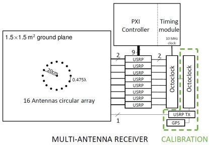
Figure 1: Measurement system schematic [43]. 16 antennas composed a UCA, and 1 antenna was located in the center of the UCA for calibration purpose. 9 USRPs were utilized to provide the 17 RF chains.

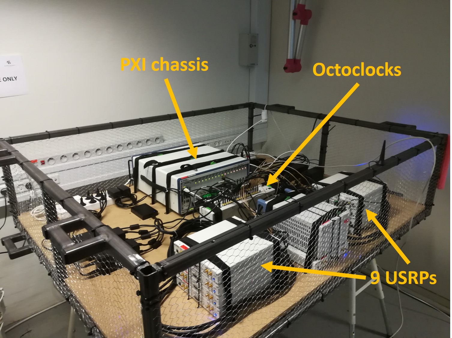
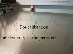
Figure 2: Measurement equipment. (a) SDR test-bed. (b) The UCA. The antenna in the center is for calibration of USRP boards.

1) Antenna array design: The sixteen-antennas UCA, as illustrated in Fig. 2(b), was designed to operate at LTE band 3 (1.8 GHz frequency band), where two LTE networks belonging to the different Danish telecom operators are located. Antenna elements, realized as simple monopoles are distributed with around 0.475 $\lambda$ spacing, corresponding to a circular radius of 20 cm and are manufactured on a large 1.5$\times$1.5 m² aluminum ground plane installed on top of the presented steel cage. The final antenna radiation pattern was simulated using computer simulation technology (CST) studio and can be well approximated by an omni-directional pattern with approximately 10^o up-tilt due to the finite size of the ground plane.

2) Calibration of USRP boards: Spatial channel characterization requires all RF chains to record the data with time, frequency and phase synchronization. Octoclocks are used to provide sufficient time and frequency alignment. However, testbeds containing multiple USRP boards suffer from the inherited lack of phase synchronization between them. Although boards are phase coherent, each of them starts with the random phase offset. Therefore, external, self-designed calibration to compensate this offset is required. The designed testbed, uses the additional antenna and a self-transmitted calibration signal for phase compensation. By transmitting a sine wave with a low power (-50 dBm) and a frequency near to the LTE band using the antenna located in the center of the array, each of the antennas forming the UCA are expected to receive the signal with the same time delay and the same phase. Assuming the received phase of one antenna as a reference, the phases of the remaining fifteen antennas can be compensated, allowing phase synchronization with less than 1^o error.

II-C Measurement campaign

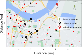
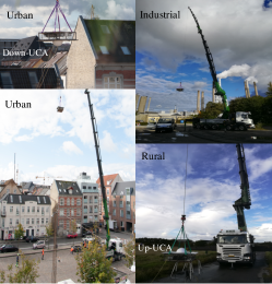
Figure 3: Measurement scenarios. (a) Measurement locations in the map. The red dots and black asterisks indicate the BS locations of two network operators, respectively. (b) Assembled setup lifted in different scenarios.

As illustrated in Fig. 3, the measurement campaign was conducted in seven different locations located in a vicinity of Aalborg, Denmark. It comprises three different measurement scenarios as described below:

• Scenario 1 - Rural: In this scenario, as illustrated in Fig. 3 and labelled as location 1, the measurement equipment was placed in a middle of the farm, where neither buildings nor trees were located in a close proximity. As the measurement location was still located close to the city, multiple cells were decodable. This scenario imitates the envisioned use cases of using UAVs for field inspection.

• Scenario 2 - Industrial: In this scenario, as illustrated in Fig. 3 and labelled as location 7, the measurement equipment was placed between many tall (up to 30 m), industrial buildings in the industrial part of the city. The measurement spot was surrounded by many elements made of concrete and represents the typical industrial environment, where UAVs are expected to be used for building inspection or for surveillance services. In addition, the average height and downtilt of the BS antennas near to the measurement locations in both industrial and rural scenarios were around 33 m and 6^∘, respectively.

• Scenario 3 - Urban: In this scenario, as illustrated in Fig. 3 and labelled as locations 2-6, the measurements were conducted in a couple of locations in a city center where the equipment was surrounded by buildings. Their average height was approximately 20 m. This scenario represents many of the envisioned use cases as for example last mile delivery services. The average height and downtilt of the BS antennas in this area were about 25 m and 6^∘, respectively.

Measurement procedure

In each of the measurement locations, the measurement procedure was as follows. The designed testbed was placed inside the steel cage and was lifted by a crane as shown in Fig. 3. The measurements were taken at nine different heights from 0 to 40 m with a 5 m step. At each measurement height, 100 ms-long measurement snapshot of the LTE network was taken five times where the reproducibility of the channel characteristics also serves as a verification of the system functionality. Considering the impact of the steel cage and its attenuation on the received signals, the same procedure was repeated twice. During the first time, the steel cage was mounted with the UCA on top of the cage, while during the second time, the UCA was located below the cage. Finally, to gather as much diverse data as possible, the same measurements were conducted twice, separately for the two network operators. Therefore, in total 2$\times$2$\times$9$\times$5$\times$7=1260 (corresponding to the number of operators, up/downwards UCA, number of measurement heights, number of repeated snapshots, number of measurement locations, respectively) measurement snapshots were recorded.

III CIR extraction and Channel APDPs

In this section, we will present the post processing procedure to extract the CIRs for the measured downlink UCA array data. Example APDPs observed at different heights in different scenarios are also illustrated. The preliminary channel characteristics observed from the APDPs are discussed.

III-A CIR extraction from raw data

The post processing procedure of extracting CIRs from the measured downlink raw data is similar to the procedure specified in [31, 44]. The main steps include i) low-pass filtering to remove possible out-of-band interferences, ii) primary synchronization exploiting the primary synchronization signals, iii) secondary synchronization utilizing the secondary synchronization signals and iv) CIR extraction by applying the inverse Fourier transform to the channel transfer functions (CTFs) obtained exploiting the cell specific signals. The improvement in this work is that before obtaining time synchronization and detecting physical cells, Bartlett beamforming was firstly conducted by combining the measured data at all the 16 antennas of the UCA. Through iteratively adapting the beamforming weights of the UCA targeting different/grid directions, the signal-to-interference-plus-noise ratio (SINR) of the received signals from cells covered by the current beam was increased due to the mitigation of inter-cell interferences, which led to a better cell detection compared to that of using a single antenna in [31]. The step iv) CIR extraction was then applied to the UCA for all the detected cells in individual measurement snapshots. Readers are referred to [31] for the detailed description of the steps of raw data processing. For each measurement snapshot lasting 0.1 second, 16$\times$200 CIRs, i.e. 200 consecutive CIRs for each of the 16 antennas of the UCA, can be extracted from the measured data for each detected cell. To avoid possible problems caused by, e.g. the warming-up stage of the USRPs, only the latter 16$\times$180 CIRs were considered for the following investigations. In addition, we denote the array CIRs extracted for a detected cell in one measurement snapshot as $h(m,t,\tau)$ where $m\in\{1,\cdots,M;M=16\}$, $t$ and $\tau$ indicates the antenna index, time and delay, respectively. The time difference between consecutive CIRs is 0.5 ms. The bandwidth of the CIR is 18 MHz with 200 delay sampling points, which corresponds to a maximum observable path delay difference of around 11 $\mu$s, i.e. 3.33 km.

III-B Example APDPs

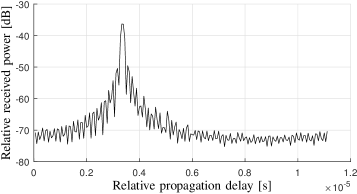
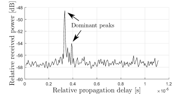
Figure 4: Example APDPs obtained in the rural scenario in location 1 as indicated in Fig. 3. (a) Height of 0 m. (b) Height of 35 m.

Multiple cells can be detected in one measurement snapshot at a certain height and location. In this section, we show some example APDPs for different heights at different scenarios. Note that the illustrated APDPs may not attributed to the same cell. Thus, in Figs. 4 to 6 the received power of an APDP at a higher height is not necessarily higher or lower than that of an APDP at a lower height. The APDPs are obtained by averaging the power delay profiles (PDPs) over time. That is, $s(m,\tau)=\frac{1}{N}\sum_{t_{1}}^{t_{N}}|h(m,t,\tau)|^{2}$ for one set of UCA array CIRs with $N=180$ in our case. For clarity, we only illustrate the APDP observed at one antenna of the UCA for a detected cell.

III-B1 Rural scenario

Fig. 4 illustrates two APDPs obtained in the rural area at location 1 as indicated in Fig. 3 at the heights of 0 and 35 m, respectively. Note that the propagation delays are relative due to the fact that the time synchronization is done offline in the CIR extraction. It can be inferred from Fig. 4 that the illustrated channel at the height of 0 m is dominant with one path (i.e., the LoS path), as the APDP has a close-to-perfectly symmetric sinc-alike shape. This is reasonable since the rural area is rather open with almost no scatterers such as tall buildings that can lead to significant path components. Moreover, the dynamic range of the APDP is high, which is mainly because the cellular BS antenna beam is always down tilted towards the ground to better serve the ground users. Fig. 4 illustrates another APDP at the height of 35 m with a smaller dynamic range, which is probably because i) the UCA was out of the main lobe of the BS, and ii) with less blockage at a higher height, interferences from other cells also increased the noise floor. However, it is obvious that at least two path components exist in the channel as indicated by the two peaks in Fig. 4. Moreover, the power difference of the two peaks is not large. This demonstrates the fact the at a higher height, the channel may not always become more LoS-alike as assumed in many other works, even in the rural area. Nevertheless, we show this APDP as a special case. Most of the channels in the rural scenario became LoS-dominant at higher heights, which we will discuss in details in Sect. V.

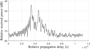
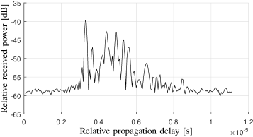
Figure 5: Example APDPs obtained in the industrial scenario in location 7 as indicated in Fig. 3. (a) Height of 0 m. (b) Height of 25 m.

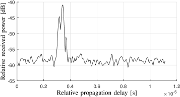
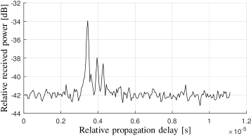
Figure 6: Example APDPs obtained in the urban scenario in location 3 as indicated in Fig. 3. (a) Height of 0 m. (b) Height of 40 m.

III-B2 Industrial scenario

Fig. 5 illustrates two APDPs measured in the industrial area at location 7 as indicated in Fig. 3 at the heights of 0 and 25 m, respectively. As illustrated in Fig. 5, multiple peaks (or path components) can already be observed in the APDP at the height of 0 m attributed to e.g. the factory buildings. At a higher height, e.g. 25 m as indicated in Fig. 5, the richness of the path components of the channel can be even higher. We postulate this is probably due to the reflections from the roofs or round walls of the factory buildings, as indicated in Fig. 3, which are visible to the UAV-UE at a properly higher height.

III-B3 Urban scenario

Fig. 6 illustrates two APDPs measured in the urban area at location 3 as indicated in Fig. 3 at the heights of 0 and 40 m, respectively. It can be observed from Fig. 6 that at the height of 0 m, multiple path components exist in the channel. Moreover, it can be inferred that the LoS path has probably been blocked as the path with the highest power is not with the minimum delay. The phenomena are understandable since there are multiple buildings in the dense urban area. Fig. 6 illustrates another example APDP at the height of 40 m, where multiple path components can still be observed. We postulate this is also attributed to the richness of scattering objects in the urban scenario.

To summarize, in this section we have shown some interesting channels measured in different scenarios at different heights. By observing the shape of the APDPs, some preliminary insights into the temporal characteristics of the channels can be appreciated. The channel at a higher height may not be always LoS dominant. Moreover, at a certain height in a specific scenario, e.g. 25 m at the industrial area, the channel may have higher richness of multipath components, due to certain physical mechanisms such as reflections from roofs and sidewalls. Note that the selected interesting/non-intuitive APDPs may not represent the general channels. To gain more detailed and general insights into the channels with high resolutions considering also the angular domain, in the sequel we implement a HRPE algorithm for all the measured downlink UCA array data, and cluster identification will be applied to the estimated channel parameters.

IV Channel parameter estimation and clustering

In this section, the high resolution estimation of channel parameters (including delays, powers and angles of multipath components) is firstly elaborated. The practical issues such as calibration and incomplete knowledge of radiation patterns are also considered carefully, which is important for the algorithm to work in practice for the measured data sets. Moreover, the reasonability of the results is not only guaranteed theoretically but also verified empirically. Based on the HRPE results obtained, a threshold-based algorithm is applied to group the channels into clusters each consisting of multipath components with similar delays and angles, to facilitate the model establishment.

IV-A High resolution channel parameter estimation

IV-A1 Signal model and physical impairments

The exploitation of the UCA makes it possible to extract the propagation channel parameters in the angular domain from the measured array CIRs. In this section, we utilize an approach which is derived based on the space-alternating generalized expectation-maximization (SAGE) principle [45] for this purpose. The SAGE algorithm has been widely used for channel parameter estimation due to its low complexity and ability to obtain HRPE results [45]. As a variant of the expectation-maximization (EM) algorithm, the SAGE algorithm includes E-steps and M-steps to achieve convergence. In the E-step, the conditional expectations of signals contributed by individual path components are calculated based on the prior information obtained in the M-step, where the channel parameters of a path are estimated using successive dimension-wise maximization-likelihood principle, and the estimated parameters are updated immediately for the following E-steps. Readers are referred to [45, 46] for the implementation details.

The underlying signal model assumed for the propagation channel is formulated as

$$h_{\text{ideal}}(t,\tau,\phi,\theta,\nu)$$ (1)

$$=\sum_{\ell=1}^{L(t)}\alpha_{\ell}(t)\delta(\tau-\tau_{\ell}(t))\delta(\phi-\phi_{\ell}(t))\delta(\theta-\theta_{\ell}(t))\delta(\nu-\nu_{\ell}(t))$$

where $L(t)$ is the total number of the propagation paths in the channel snapshot observed at time instant $t$; $\alpha_{\ell}(t)$, $\tau_{\ell}(t)$, $\phi_{\ell}(t)$, $\theta_{\ell}(t)$ and $\nu_{\ell}(t)$ represent the complex amplitude, delay, azimuth angle, elevation angle and Doppler frequency of the $\ell$th path component, respectively, and $\delta(\cdot)$ indicates the Dirac delta function. Note that in the measurement campaign, we assume the channel parameters are stationary in each measurement snapshot as the UCA was kept almost still when collecting the downlink data. In other words, we assume the path number and channel parameters, e.g. delays and angles, of the propagation channel between a BS and the UCA do not change during one measurement snapshot. For different measurement snapshots or detected cells $L$ can be different. The reasons for including Doppler frequencies in the signal model are two folds. One is that small movement of UCA caused by, e.g. the wind etc., was inevitable. The other reason is that there may exist frequency shifts in oscillators of BSs and the UCA measurement system, which could cause “fake” Doppler frequencies. Therefore, the empirically received UCA CIRs according to (1) with additive white Gaussian noise is formatted as

$$\begin{aligned} &h(m,t,\tau)\\ &=\sum_{\ell=1}^{L}\alpha_{\ell}\mathbf{a}(\phi_{\ell},\theta_{\ell})\odot\mathbf{r}_{\ell}(\phi_{\ell},\theta_{\ell})u(\tau-\tau_{\ell})e^{j2\pi\nu_{\ell}t}+n(m,t,\tau)\end{aligned}.$$ (2)

In (2), $\mathbf{a}(\phi_{\ell},\theta_{\ell})$ is the so-called steering vector, a complex vector of dimension $M\times 1$ that can be readily formatted according to the UCA geometry considering the path impinging with azimuth $\phi_{\ell}$ and elevation $\theta_{\ell}$. Due to the differences among the antenna radiation patterns and the different blockages for individual antennas caused by e.g. the assemble setup, another vector of dimension $M\times 1$, $\mathbf{r}_{\ell}(\phi_{\ell},\theta_{\ell})\triangleq[r_{\ell,1}(\phi_{\ell},\theta_{\ell}),\cdots,r_{\ell,M}(\phi_{\ell},\theta_{\ell})]^{T}$ has to be included to compensate the received power differences among antennas. $T$ and $\odot$ indicate the matrix transpose operation and Hadamard product (element-wise multiplication), respectively. Moreover, $u(\tau)$ is the shape function introduced by the measurement system. Ideally, $u(\tau)$ is a sinc function if there is only the effect of limited bandwidth (18 MHz in our case). However, the measurement system usually has other system imperfections, which compositely makes $u(\tau)$ very different from an ideal sinc function. As for $\mathbf{r}_{\ell}$, Fig. 7 illustrates the received powers of the dominant path at the 16 antennas, obtained from a rural (close to LoS) $h(m,t,\tau)$ as in (2). Ideally, the powers of the LoS path received at different antennas should be the same or with little difference. However, it can be observed from Fig. 7 that the received powers at different antennas can be very different, which we postulate is mainly due to the radiation pattern difference and blockage difference across the UCA elements. This imperfection problem has to be considered when performing the parameter estimation. One may think that this can be calibrated by measuring the patterns in a anechoic chamber. However, the difficulty is to make sure the UCA has the same status in the chamber to that in the measurement campaign. The rotation must refer to the phase center of the UCA (which is physically unknown), and the other 15 antennas should be kept active when one element is measured. The practical difficulties make it almost impossible to obtain good calibration results of $\mathbf{r}_{\ell}$ that can improve the estimation. The model mismatch will lead to failures both in the E-steps and M-steps, and results show that the original SAGE algorithm does not work as many more spurious (ghost) path-components has been estimated if $\mathbf{r}$ is omitted as $\mathbf{1}$-vector. This mean that we must carefully consider the physical impairments, i.e. $u(\tau)$ and $\mathbf{r}_{\ell}$, in the parameter estimation to obtain realistic results.

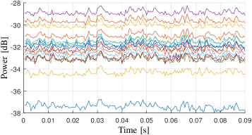
Figure 7: The received power at the 16 antennas for the same path component. This example is obtained from a rural data. The different lines represent the received power at the 16 antennas, respectively.

IV-A2 Calibrate $u(\tau)$

The following operations were conducted in order to obtain $u(\tau)$ as close as possible to that in the field measurements. The same version of the standard LTE frequency division duplex (FDD) signals transmitted by the BSs in the measurement campaign were generated. The generated signals were then fed to and transmitted by a USRP in the laboratory. The type of the USRP was the same to that used for the UCA, and the center frequencies and bandwidth were set identical to that of the commercial networks, respectively. Moreover, the Tx RF port of this USRP was directly connected to the Rx RF port of the primary USRP (which was connected to the first antenna of the UCA in the measurements). The cable used in the field measurements was still used for the direct connection with a necessary attenuator added. The transmitted “downlink LTE signals” were then collected by the primary USRP using the exactly same configuration to that for sounding the live LTE signals. Further, we exploited the same procedure as elaborated in Sect. III-A to extract the CIRs $h_{\text{d}}(t,\tau)$ from the received data. To remove the effect of thermal noise and oscillator inaccuracy in the USRP, we firstly estimated the Doppler frequency caused by the oscillator inaccuracy as

$$\hat{\nu}_{\text{d}}=\arg\max_{\nu}\left|\sum_{t=t_{1}}^{t_{N_{\text{d}}}}e^{-j2\pi\nu t}h_{\text{d}}(t,\hat{\tau}_{\text{d}})\right|^{2},$$ (3)

$$\hat{\tau}_{\text{d}}=\arg\max_{\tau}\sum_{t=t_{1}}^{t_{N_{\text{d}}}}\left|h_{\text{d}}(t,\tau)\right|^{2}$$ (4)

where $N_{\text{d}}$ is the number of CIRs utilized. Then $u(\tau)$ is estimated by coherently combining the CIRs as

$$\begin{aligned} \hat{u}(\tau)=\sum_{t=t_{1}}^{t_{N_{\text{d}}}}h_{\text{d}}(t,\tau)e^{-j2\pi\nu t}\end{aligned}.$$ (5)

Normalization of power and phase and shifting delay to 0 were also applied afterwards. Fig. 8 illustrates the estimated $\hat{u}(\tau)$ using $N_{\text{d}}=400$ CIRs. The “fake” Doppler frequency was estimated as around -12 Hz. A standard 18 MHz bandwidth-limited sinc function is also plotted. Their delays are shifted from 0 for a better presentation in Fig. 8. It can be observed that the system effects of the USRP utilized in the measurements is indeed non-negligible. The obtained close-to-noise-free $\hat{u}(\tau)$ makes it possible to remove/calibrate the system effects of $u(\tau)$.

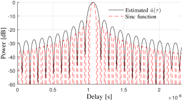
Figure 8: The shape of the estimated $u(\tau)$ of the USRP and the shape of standard bandwidth-limited sinc function.

IV-A3 Deal with unknown $\mathbf{r}_{\ell}$

: A novel strategy is proposed to deal with the unknown $\mathbf{r}_{\ell}$. The main idea is to firstly estimate only amplitudes, delays and Doppler frequencies of path components at individual antennas, and angular parameters are then estimated exploiting the complex amplitudes of 16 antennas. Specifically, in the E-step, the expectation of the hidden signals contributed by the $\ell$th path and received by the $m$th antenna is calculated as

$$\hat{h}_{m,\ell}(t,\tau)=h(m,t,\tau)-\sum_{q\in\mathcal{L},q\neq\ell}\alpha_{m,q}^{\prime}u(\tau-\tau_{q}^{\prime})e^{j2\pi\nu_{q}^{\prime}t}$$ (6)

where $\alpha_{m,q}^{\prime}$, $\tau_{q}^{\prime}$ and $\nu_{q}^{\prime}$ are the estimated complex amplitude, delay and Doppler frequency respectively in the previous M-step for the $q$th path received at the $m$th antenna, and $\mathcal{L}=\{1,\cdots,L\}$ is the set of all path indices. In the next M-step, the maximum-likelihood estimations are formatted as

$$\begin{aligned} (\tau_{\ell}^{\prime},\nu_{\ell}^{\prime})=\arg\max_{\tau_{0},\nu}\left\{\sum_{m=1}^{M}\left|\sum_{t_{1}}^{t_{N}}e^{-j2\pi\nu t}\int u^{*}(\tau-\tau_{0})h_{m,\ell}(t,\tau)d\tau\right|^{2}\right\}\end{aligned}$$ (7)

$$\alpha_{m,\ell}^{\prime}=\frac{1}{N\int|u(\tau)|^{2}d\tau}\sum_{t_{1}}^{t_{N}}e^{-j2\pi\nu_{\ell}^{\prime}t}\int u^{*}(\tau-\tau_{\ell}^{\prime})h_{m,\ell}(t,\tau)d\tau$$ (8)

where ^∗ indicates the conjugate of the argument. With convergence, the parameters $\boldsymbol{\hat{\alpha}}_{\ell}\triangleq[\hat{\alpha}_{m,1},\cdots,\hat{\alpha}_{m,\ell}]^{T}$, $\hat{\tau}_{\ell}$ and $\hat{\nu}_{\ell}$ are obtained. The azimuths, elevations and amplitudes of individual paths are estimated as

$$\begin{aligned} (\hat{\phi}_{\ell},\hat{\theta}_{\ell})=\frac{1}{M}\arg\max_{\phi,\theta}\boldsymbol{\hat{\alpha}}_{\ell}^{T}\mathbf{a}^{*}(\phi,\theta)\end{aligned},$$ (9)

$$\begin{aligned} \hat{\alpha}_{\ell}=\frac{1}{M}\boldsymbol{\hat{\alpha}}_{\ell}^{T}\mathbf{a}^{*}(\hat{\phi}_{\ell},\hat{\theta}_{\ell})\end{aligned}.$$ (10)

The final parameter set obtained for one measurement snapshot is denoted as $\hat{\boldsymbol{\Theta}}=[\hat{\alpha}_{\ell},\hat{\tau}_{\ell},\hat{\phi}_{\ell},\hat{\theta}_{\ell};\ell\in\mathcal{L}]$. Moreover, it is essential to determine an appropriate $L$ (that can change for different snapshots or cells) to avoid over-estimation. The Akaike information criterion (AIC) principle [47, 48] is exploited where the $L$ that leads to the minimum AIC is used, which is equivalently to find the number of estimated paths with signal-to-noise-ratio (SNR) above a certain threshold [48]. Therefore, in practice an adequately large number of paths are firstly estimated. $L$ is chosen as the number of paths with powers above the noise floor, and the estimation is reperformed with the determined $L$ to obtain final estimation results.

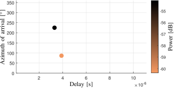
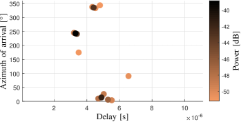
Figure 9: Example HRPE results for the measured channels. (a) The rural channel as indicated in Fig. 4. (b) The industrial channel as indicated in Fig. 5.

Fig. 9 illustrates two example HRPE estimation results for the UCA CIRs snapshots in Fig. 4 and Fig. 5, respectively. It can be observed that the number of paths estimated in the rural example is much lower than that of the industrial example. Moreover, in the rural example, the two paths have no surrounding paths in their near regions in terms of delay and angle. As a comparison, groups of paths with similar delays and angles can be found in Fig. 5 in the industrial example, although the well-separated single paths also exist. This is consistent with the intuition that richer number of scatters can result in a richer amount of paths, and sometimes a surface or open area can lead to a single path considering the finite intrinsic resolution ability achieved by the measurement system. To further empirically check the estimation results, as illustrated in Fig. 10, we compared the azimuth angles of the dominant paths estimated for individual cells detected at different heights and the corresponding geographical LoS azimuth angles (with north direction as 0^∘) calculated according to the physical locations of BSs and the UCA in the rural scenario. It can be observed from Fig. 10 that the offsets are rather stable inside each height. The change between different heights is due to the practically inevitable rotation of the UCA when it was lifted up to another height. Therefore, we do consider the HRPE results obtained in our work are realistic in both the theoretical and empirical senses.

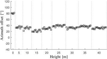
Figure 10: Offsets between the dominant azimuths estimated and the corresponding geographically LoS azimuths for individual cells detected in the rural scenario. The vertical dotted-lines separate the cells detected at different heights.

IV-B Cluster identification

The concept of channel clustering has been widely used to compromise between the model complexity and accuracy of spatial channels. A cluster is considered as a group of multipath components with similar delays and/or angles. It is essential to utilize an automatic algorithm to identify the clusters of a large amount of spatial channels available. Different approaches, e.g. K-Power-Means (KPM) [49, 50], image-processing-based methods [51, 52] and several others [53, 54] can be found in the literature. In this work, we utilize the multipath component distance (MCD)-threshold based principle [55]. The reasons are as follows: i) Based on the observation of the HRPE results obtained for the measured channels, it is found that different path-groups are quite well separated with paths confined in a certain delay-angle region as exemplified in Fig. 9. ii) In the threshold-based algorithm, no initializations or prior assumptions of cluster centroids, cluster number, paths distributions, etc. are required. The optimum threshold is physically linked to the cluster size or distribution. The investigations in [56, 54] have also shown the performance enhancement of the threshold-based algorithm compared to Gaussian-mixture-model (GMM) [54], KPM [49] and KMeans [53].

The MCD has been exploited to replace the Euclidean distances in cluster identification due to its significant performance improvement [57], which was firstly introduced and discussed in [58] to quantify the separations of multiple paths in multiple parameter domains. The MCDs in delay and angular domains are calculated differently. Specifically, the angular MCD between the $i$th and $j$th path components is calculated as

$$\text{MCD}_{\text{Tx/Rx},ij}=\frac{1}{2}\Biggl{|}\begin{pmatrix}\sin\theta_{i}\cos\phi_{i}\\ \sin\theta_{i}\sin\phi_{i}\\ \cos\theta_{i}\end{pmatrix}-\begin{pmatrix}\sin\theta_{j}\cos\phi_{j}\\ \sin\theta_{j}\sin\phi_{j}\\ \cos\theta_{j}\end{pmatrix}\Biggl{|}$$ (11)

for Tx and Rx sides, separately. The delay MCD is calculated as

$$\text{MCD}_{\tau,ij}=\frac{|\tau_{i}-\tau_{j}|}{\tau_{\zeta}}$$ (12)

with $\tau_{\zeta}$ as a scaling factor for delay. Note that the calculation in (12) is different from the original/widely-used definition of delay MCD, e.g. in [49, 56]. In the original definition, the scaling factor is subject to the maximum difference and standard deviation of path delays in a channel snapshot. This means that the scaling factor can change arbitrarily, e.g., if a cluster with a long delay exists or all the clusters (well separated in angular domain) have similar delays. However, in the same scenario clusters probably have similar physical sizes, thus it may lead to unrealistic identification results. In (12), $\tau_{\zeta}$ is selected to make the angular MCD and delay MCD of the maximum angle and delay separateness inside clusters of the same scenario be the similar/same magnitudes, which is consistent with the threshold principle. The overall MCD is then calculated as

$$\begin{aligned} \text{MCD}_{ij}=\sqrt{\text{MCD}_{\text{Tx},ij}^{2}+\text{MCD}_{\text{Rx},ij}^{2}+\text{MCD}^{2}_{\tau,ij}}\end{aligned}.$$ (13)

It is worth noting that due to the low elevation-sensitivity of UCA and the fact that the horizontal distances between the UCA and detected cells are gernerall large causing similar and small elevation angles of paths, we omit $\theta$ in the calculation of (11). Moreover, since the angular information at the BS side is unknown, we also omit $\text{MCD}_{\text{Tx},ij}$ in (13). In addition, the centroid $\mu_{c}\triangleq[\mu_{\tau},\mu_{\phi}]$ of a cluster is calculated as

$$\mu_{\tau}=\frac{\sum_{\ell\in\mathcal{L}_{c}}|\alpha_{\ell}|^{2}\tau_{\ell}}{\sum_{\ell\in\mathcal{L}_{c}}|\alpha_{\ell}|^{2}},\quad\mu_{\phi}=\text{ang}\{{\sum_{\ell\in\mathcal{L}_{c}}|\alpha_{\ell}|^{2}e^{j\phi_{\ell}}}\}$$ (14)

where $\mathcal{L}_{c}$ is the set containing the path indices belong to the concerned cluster, and $\text{ang}\{\cdot\}$ is the phase angle of the argument.

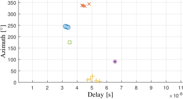
Figure 11: Identified clusters for the channel as illustrated in Fig. 9.

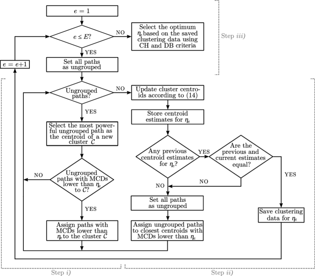
Figure 12: Cluster identification procedure applied.

The block diagram in Fig. 12 illustrates the threshold-based cluster identification for the estimated $\hat{\boldsymbol{\Theta}}$, which is similar to the procedure as proposed in [59]. Briefly , i) the path component with the highest power is chosen as the first cluster centroid, and the path components with MCDs less or equal to the pre-defined threshold $\eta_{e}$ are considered as belonging to this cluster. The same procedure continues for the residual paths until all the paths have been concerned. ii) Then the centroids of the grouped clusters are updated using (14), and the threshold-based path-assignment is re-performed referring to the updated cluster centroids. Note that i) is also required if there exist paths belonging to none of the updated centroids. The identified clusters are obtained for this $\eta_{e}$ after several iterations achieving convergence. iii) It is essential to determine $\eta_{e}$ for the cluster identification. We exploit the same approach as proposed in [49] to find the optimum $\eta_{e}$, i.e. the optimum cluster identification. That is, i) and ii) are performed for different candidate $\eta_{e}$, with $e=1,2,\dots,E$. The optimum $\eta_{e}$ is chosen as the one that leads to the optimum cluster identification, by evaluating the inter-cluster separateness and intra-cluster compactness using the Caliñski-Harabasz (CH) index and Davies-Bouldin (DB) criterion. Fig. 11 illustrates the identified clusters for the example channel as illustrated in Fig. 9. It can be observed that multiple clusters are well identified. Note that we still term the “cluster” with only one path as a “cluster” for convenience, although clusters are usually considered with multiple path components. Based on the cluster identification results, spatial channel models will be elaborated in the sequel.

V Spatial Channel Characteristics

Based on the cluster identification results, the spatial channel characteristics extracted in different scenarios are illustrated in this section. The composite parameters, e.g. the composite delay spread and azimuth spread, as well as cluster-level parameters, e.g. the number of clusters, intra-cluster delay spread, intra-cluster azimuth spread, cluster power ratio, etc. are thoroughly investigated. For each parameter, a “boxplot” figure, e.g. Fig. 13, is used to show the parameter variations at different heights in the three scenarios. The parameter set is consistent with the standard spatial channel modelling methodology as specified in [42]. For example, with composite spreads, cluster number, cluster power ratio and cluster offsets known, locations and relative powers of individual clusters can be generated. According to the intra-cluster spreads, the path distributions inside clusters can be further reproduced. Reader are referred to [42] for detailed procedures of channel reproduction stochastically.

V-A Composite delay spread $\sigma_{\tau}$ and azimuth spread $\sigma_{\phi}$

As commonly characterized [44], the root-mean-square (RMS) delay spread of a channel can be calculated according to the HRPE $\hat{\boldsymbol{\Theta}}$ as

$$\sigma_{\tau}=\sqrt{\overline{{\tau}^{2}}-\overline{\tau}^{2}}$$ (15)

with

$$\begin{aligned} \overline{{\tau}^{2}}=\frac{\sum_{\ell\in\mathcal{L}}\left|\alpha_{\ell}\right|^{2}\cdot\tau_{\ell}^{2}}{\sum_{\ell\in\mathcal{L}}\left|\alpha_{\ell}\right|^{2}},\quad\overline{\tau}=\frac{\sum_{\ell\in\{\mathcal{L}\}}\left|\alpha_{\ell}\right|^{2}\cdot\tau_{\ell}}{\sum_{\ell\in\{\mathcal{L}\}}\left|\alpha_{\ell}\right|^{2}}\end{aligned}.$$ (16)

The RMS azimuth spread is calculated differently as specified in [42]

$$\begin{aligned} \sigma_{\phi}=\sqrt{-2\mathrm{log}\left(\left|\frac{\sum_{\ell\in\mathcal{L}}\mathrm{exp}(j\phi_{\ell})\cdot\left|\alpha_{\ell}\right|^{2}}{\sum_{\ell\in\mathcal{L}}\left|\alpha_{\ell}\right|^{2}}\right|\right)}\end{aligned}.$$ (17)

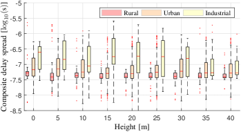
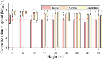
Figure 13: The composite delay spreads and composite azimuth spreads observed in the three scenarios. (a) Composite delay spreads $\sigma_{\tau}$. (b) Composite azimuth spreads $\sigma_{\phi}$.

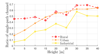
Figure 14: Ratios of single-path channels at different heights in the three scenarios.

Fig. 13 illustrates the observed composite delay and azimuth spreads, both indicated in logarithm scales, for the three scenarios. Note that a channel may be estimated with only one path whose spreads are 0, therefore such CIRs are excluded when plotting Fig. 13. The ratios of the single-path channels, defined as the ratio of the number of the channels with only one path to the number of all the channels, at different heights in the three scenarios are illustrated in Fig. 14. It can be observed that generally the composite spreads in the rural scenario are the smallest, and the ratios of single-path channels are the largest (with a ratio of 45% already at 0 m). This is consistent with the fact that the rural scenario is quite open. As a contrast, the industrial scenario basically has the largest spreads and smallest ratios of single-path channels, due to the many concrete elements existing. Moreover, it can be observed that the composite spreads in one scenario have the trends to be smaller at a higher height, although they can be larger at some higher heights, e.g. 25 m in the industrial scenario and 30 m in the urban scenario. Meanwhile, the ratio of single path channel becomes larger with increasing heights. The phenomena are reasonable since a higher height can in principle result in a less complicated channel, whereas the signals from the building roofs or sidewalls may cause larger spreads at a proper height in the urban and industrial scenarios.

V-B Cluster power ratio $K$ and number of clusters $C$

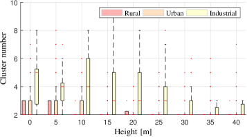
Figure 15: The numbers of clusters $C$ for multiple-clusters channels at different heights in the three scenarios.

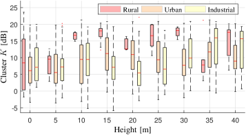
Figure 16: Cluster power ratios $K$ at different heights in the three scenarios.

For a channel $\hat{\boldsymbol{\Theta}}$, $C$ clusters are identified and sorted with power-descending order. The cluster power ratio $K$ is defined as

$$K=\frac{p_{1}}{\sum_{c=2}^{C}p_{c}},$$ (18)

$$\begin{aligned} p_{c}=\sum_{\ell\in\mathcal{L}_{c}}|\alpha_{\ell}|^{2}\end{aligned}.$$ (19)

$K$ demonstrates the importance of the dominant cluster in the channel. A very high $K$ means that the other clusters can be negligible for communications, whereas a small $K$ means that the other clusters can be potentially exploited for communications as they contain non-negligible power. Note that $C$ can be 1 for some channels. Thus, single-cluster channels are not considered when calculating $K$. Figs. 15 and 16 illustrate the number of clusters and the cluster power ratios $K$ for multiple-clusters channels at different heights in the three scenarios. The corresponding ratios of single-cluster channels, defined as the ratio of the number of the channels with only one cluster to the number of all the channels, are also illustrated in Fig. 17. It can be observed from Fig. 15 that the number of clusters becomes smaller with increasing heights for all the three scenarios. The number of clusters in the industrial scenario is the largest among the three scenarios, which is also consistent with its largest composite spreads as illustrated in Fig. 13. As for $K$, it can be observed from Fig. 16 that it is not large at lower heights, i.e. 0 and 5 m, for all the scenarios. In the rural scenario, $K$ basically increases with increasing heights. However, $K$ becomes much lower at 35 m as an exception. We have illustrated the type of APDPs in Fig. 4, which is probably because the power of the LoS cluster decreases due to the downtilt BS antenna pattern, and the reflected component(s) from a certain scatterer that can be detected by the UAV-UE at this height have non-negligible power(s). For the urban and industrial scenarios, $K$ has similar behaviours. That is, it increases, then decreases and increases again with increasing heights. We postulate this is mainly because at middle heights, e.g. around 20-25 m in the industrial scenario, building roofs or sidewalls in both scenarios can lead to clusters with relatively high powers. Specially, the median of $K$ can be lower as around 5 dB in the industrial scenario at the height of 20 m. Nevertheless, it can be observed from Fig. 17 that the ratio of single cluster channel tends to increase with increasing heights for all the three scenarios (where the rural scenario has the largest ratios). This indicates that most of the channels at a higher height in all the three scenarios are with smaller spreads.

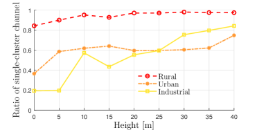
Figure 17: Ratios of single-cluster channels at different heights in the three scenarios.

V-C Intra-cluster delay spread $\sigma_{\tau_{c}}$ and azimuth spread $\sigma_{\phi_{c}}$

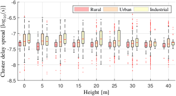
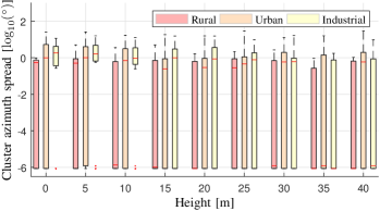
Figure 18: The intra-cluster delay spreads and azimuth spreads observed in the three scenarios. (a) Intra-cluster delay spreads $\sigma_{\tau_{c}}$. (b) Intra-cluster azimuth spreads $\sigma_{\phi_{c}}$.

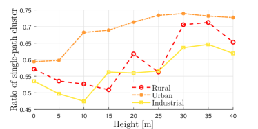
Figure 19: Ratios of single-path clusters at different heights in the three scenarios.

The intra-cluster delay spread and azimuth spread of an identified cluster are calculated using (15) and (17), respectively, with $\mathcal{L}$ replaced with $\mathcal{L}_{c}$. Similarly, clusters with a single path are excluded. Fig. 18 illustrates the observed intra-cluster delay and azimuth spreads, both indicated in logarithm scales, for the three scenarios. The ratios of single-path clusters, defined as the ratio of the number of the clusters with only one path to the number of all the clusters, are illustrated in Fig. 19. It can be observed from Fig. 18 that the intra-cluster spreads are the smallest in the rural scenario, and they have weak dependence with heights. We conjecture this is because the rural scenario is very open, and most of the clusters are attributed to the LoS links. In the urban scenario, the intra-cluster spreads basically decrease with increasing heights. However, in the industrial scenario, it can be observed that the intra-cluster delay spreads can become larger at a certain height, e.g. at 25 m, although the overall trend is to decrease with increasing heights. We postulate this is mainly because the urban scenario and the industrial scenario have different types of buildings. In the industrial scenarios, several tall building with round sidewalls can exist in a certain region together with some lower building roofs, which can result in a cluster of path components with a larger intra-cluster delay spread. However, in the urban scenario, there are no round and tall concrete-elements, and houses roofs are usually spire-alike with their slopes towards different directions. Thus, clusters, each caused by a single roof, with smaller spreads both in delay and azimuth are more possible to occur. This can also be inferred from Fig. 19 that the ratio of single-path clusters in the urban scenario is larger than that in the industrial scenario in most cases. Besides, the single-path-cluster ratios basically increase with increasing heights in all the three scenarios. It is also worth noting that the rural scenario do not have the highest ratios as those illustrated in Fig. 14 or Fig. 17. This is because a channel in the urban and industrial scenarios is more possible to have multiple clusters, among which several single-path clusters can exist.

V-D Inter-cluster delay offsets $\tau_{\text{o}}$, azimuth offsets $\phi_{\text{o}}$ and power offsets $p_{\text{o}}$

The inter-cluster delay/azimuth offsets are calculated as the differences between the mean delays/azimuths of the non-dominant clusters and the mean delay/azimuth of the dominant cluster of a channel. They indicate the separateness of the multiple clusters in terms of delay and azimuth. For example, a large azimuth offset means that the spatial diversity may be exploited using multiple horn antennas at the UAV-UE side.

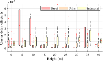
Figure 20: The inter-cluster delay offsets of multiple-clusters channels at different heights in the three scenarios.

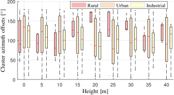
Figure 21: The inter-cluster azimuth offsets of multiple-clusters channels at different heights in the three scenarios.

Fig. 20 illustrates the delay offsets at different heights in the three scenarios. Note that they are only calculated for the channels with multiple clusters. It can be observed from Fig. 20 that in both the industrial scenarios and the urban scenarios, delay offsets become larger with increasing heights. This is reasonable since with a higher height, it is more possible that farther objects can also contribute to the received signals. However, it is obvious that in the urban scenario the delay offsets do not increase as fast as that observed in the industrial scenario. We postulate this is also due to the different types of buildings in the two scenarios. With very tall concrete elements in the industrial scenario, path components with much farther delays can be observed with higher heights. As for the rural scenario, delay offsets are quite small at most of the heights as there is no building in a close proximity in the open field, except that in some cases path components from very-far objects can lead to very large delay offsets. Fig. 21 illustrates the azimuth offsets at different heights in the three scenarios. It can be observed that there are no certain trends can be observed with respect to heights. Overall, the deviations of the azimuth offsets in the urban scenario are the largest due to its high density of buildings therein. Moreover, the azimuth offsets are usually large as above 60^∘, which indicates the multiple clusters are well separated in the azimuth domain.

We also inspected the power decay behaviours of clusters with respect to their delays and do not find certain dependences, e.g. exponential decay, between cluster powers and cluster delays. We postulate this is due to the fact that the powers of clusters not only related to the propagation distances but also the radiation patterns of the cellular BSs. It is probably random that a cluster may be caused by the main lobe or sidelobes of a BS. Nevertheless, we calculated the inter-cluster power offsets as the difference between the power in dB of the dominant cluster and the powers in dB of the other non-dominant clusters. Fig. 22 illustrates the power offsets at different heights in the three scenarios. The consistency between Fig. 22 and Fig. 16 can be well observed. For example, in the rural scenario, the power offsets are quite high at above 10 m (except 35 m), which results in high $K$’s at these heights in Fig. 16. In the industrial scenario, the power offsets at 20 m have the lowest values among all the heights, which corresponds to the lowest cluster $K$, as illustrated in Fig. 16, for the industrial scenario.

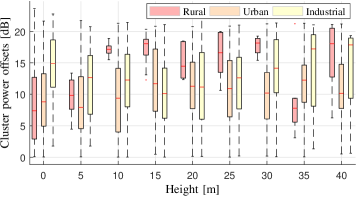
Figure 22: The inter-cluster power offsets of multiple-clusters channels at different heights in the three scenarios.

Table I: Statistics extracted for the spatial channels at different heights in the three scenarios. The three lines of parameter values from top to bottom in each cell correspond to the rural, urban and industrial scenarios, respectively. $r_{1}$, $r_{2}$ and $r_{3}$ represent the ratios of single-path channels, single-cluster channels and single-path clusters, respectively. Due to space limitation, we do not include the 25th-percentile, 75th-percentile, minimum and maximum of each parameter sample, which can be found in the “boxplot” figures, e.g., Fig. 16 for cluster K.

	Channel parameter values: (mean, std.)
Height $[\text{m}]$	Ratios ($r_{1}$; $r_{2}$; $r_{3}$)	Composite delay spreads [$\log_{10}(\text{s})$]	Composite azimuth spreads [$\log_{10}(^{\circ})$]	Cluster number	Cluster $K$ [dB]
0	(0.45; 0.84; 0.57) (0.17; 0.36; 0.59) (0.06; 0.19; 0.54)	(-7.24, 0.51) (-7.12, 0.36) (-6.74, 0.40)	(-1.0, 2.9) (1.1, 1.8) (0.6, 2.3)	(2.3, 0.5) (2.7, 1.1) (4.3, 1.9)	(9.0, 8.4) (6.5, 5.1) (8.6, 6.3)
5	(0.46; 0.90; 0.54) (0.26; 0.59; 0.60) (0.10; 0.20; 0.50)	(-7.23, 0.64) (-7.10, 0.43) (-6.75, 0.47)	(-1.6, 3.1) (0.6, 2.2) (0.9, 2.2)	(2.5, 0.5) (2.7, 1.2) (3.7, 1.3)	(8.4, 3.3) (6.8, 5.8) (7.0, 5.6)
10	(0.48; 0.95; 0.53) (0.38; 0.62; 0.68) (0.24; 0.57; 0.47)	(-7.33, 0.31) (-7.16, 0.44) (-7.08, 1.78)	(-2.9, 3.1) (0.1, 2.7) (0.1, 2.3)	(2.2, 0.4) (2.4, 0.8) (3.9, 1.9)	(16.5, 1.1) (8.6, 6.4) (8.4, 7.1)
15	(0.43; 0.93; 0.51) (0.48; 0.64; 0.69) (0.27; 0.43; 0.56)	(-7.43, 0.23) (-7.29, 0.37) (-7.22, 2.81)	(-2.6, 3.2) (-1.0, 3.1) (0.4, 2.5)	(2.0, 0.0) (2.2, 0.5) (3.7, 2.0)	(17.3, 2.6) (11.0, 5.5) (7.2, 6.4)
20	(0.58; 0.97; 0.62) (0.55; 0.60; 0.71) (0.37; 0.55; 0.56)	(-7.40, 0.18) (-7.24, 0.43) (-7.09, 2.44)	(-3.6, 3.0) (-1.1, 3.2) (-0.6, 3.2)	(2.2, 0.4) (2.2, 0.5) (3.7, 1.5)	(13.9, 1.9) (10.7, 5.3) (6.0, 6.0)
25	(0.52; 0.97; 0.56) (0.57; 0.60; 0.73) (0.30; 0.60; 0.57)	(-7.39, 0.21) (-7.20, 0.42) (-7.21, 2.61)	(-2.7, 3.1) (-1.1, 3.1) (-0.5, 3.0)	(2.0, 0.0) (2.4, 0.7) (3.5, 1.8)	(16.2, 4.0) (9.7, 6.1) (7.8, 6.1)
30	(0.68; 0.98; 0.71) (0.62; 0.60; 0.74) (0.58; 0.75; 0.64)	(-7.44, 0.23) (-7.18, 0.83) (-6.90, 0.50)	(-3.3, 3.0) (-1.2, 3.2) (-1.6, 3.5)	(2.0, 0.0) (2.3, 0.6) (2.8, 1.4)	(17.7, 1.7) (8.7, 5.2) (10.9, 6.4)
35	(0.69; 0.98; 0.71) (0.62; 0.62; 0.73) (0.51; 0.80; 0.65)	(-7.35, 0.26) (-7.20, 0.44) (-7.01, 0.47)	(-4.1, 2.9) (-1.6, 3.3) (-2.6, 3.5)	(2.0, 0.0) (2.3, 0.7) (2.3, 0.4)	(9.1, 6.4) (10.8, 4.8) (13.6, 6.8)
40	(0.64; 0.98; 0.65) (0.64; 0.75; 0.73) (0.50; 0.84; 0.62)	(-7.37, 0.15) (-7.21, 0.37) (-7.10, 0.36)	(-3.3, 3.1) (-1.7, 3.3) (-2.1, 3.3)	(2.1, 0.4) (2.3, 0.8) (2.3, 0.5)	(15.1, 5.4) (9.7, 5.0) (12.2, 6.6)
Height $[\text{m}]$	Cluster azimuth spreads [$\log_{10}(^{\circ})$]	Cluster delay spreads [$\log_{10}(\text{s})$]	Cluster delay offsets [$\log_{10}(\text{s})$]	Cluster azimuth offsets [∘]	Cluster power offsets [dB]
0	(-2.1, 2.7) (-1.6, 3.0) (-1.0, 2.7)	(-7.38, 0.24) (-7.20, 0.31) (-7.17, 0.22)	(-5.90, -5.73) (-6.60, -6.59) (-6.15, -6.35)	(103, 46) (119, 49) (113, 42)	(8.4, 7.1) (9.1, 5.3) (14.5, 5.4)
5	(-2.3, 3.0) (-1.3, 2.8) (-1.0, 2.7)	(-7.47, 0.23) (-7.18, 0.28) (-7.25, 0.30)	(-5.49, -5.60) (-6.49, -6.47) (-6.06, -6.11)	(91, 25) (112, 51) (106, 41)	(9.6, 2.8) (8.7, 5.3) (11.6, 5.4)
10	(-3.2, 2.9) (-2.1, 3.1) (-1.0, 2.5)	(-7.40, 0.18) (-7.24, 0.29) (-7.30, 1.36)	(-5.63, -5.67) (-6.41, -6.28) (-5.94, -6.04)	(91, 35) (114, 52) (104, 36)	(17.2, 1.1) (9.3, 5.8) (11.5, 5.7)
15	(-3.4, 3.0) (-2.9, 3.0) (-1.7, 3.1)	(-7.37, 0.10) (-7.33, 0.21) (-7.50, 2.20)	(-6.67, -6.61) (-6.43, -6.34) (-5.93, -5.92)	(132, 25) (110, 53) (105, 41)	(17.3, 2.6) (11.8, 5.5) (10.2, 5.2)
20	(-3.9, 2.9) (-2.8, 3.1) (-1.8, 3.1)	(-7.38, 0.14) (-7.32, 0.21) (-7.39, 1.86)	(-6.80, -6.68) (-6.33, -6.25) (-5.89, -5.87)	(154, 34) (100, 53) (86, 44)	(15.1, 3.0) (11.2, 5.0) (11.1, 5.9)
25	(-3.0, 3.0) (-2.7, 3.1) (-2.0, 3.0)	(-7.36, 0.15) (-7.32, 0.22) (-7.51, 2.24)	(-6.82, -6.69) (-6.27, -6.19) (-5.89, -6.05)	(121, 60) (96, 55) (103, 48)	(16.2, 4.0) (10.6, 5.8) (11.6, 5.3)
30	(-3.5, 2.9) (-2.6, 3.2) (-2.4, 3.1)	(-7.39, 0.17) (-7.36, 0.82) (-7.26, 0.33)	(-7.20, -8.33) (-6.23, -6.24) (-5.90, -6.20)	(139, 20) (104, 54) (108, 36)	(17.7, 1.7) (9.8, 5.0) (13.8, 5.6)
35	(-4.5, 2.6) (-2.9, 3.2) (-4.0, 2.9)	(-7.39, 0.13) (-7.35, 0.27) (-7.28, 0.17)	(-5.92, -5.81) (-6.23, -6.25) (-5.76, -5.99)	(103, 25) (103, 55) (91, 33)	(9.1, 6.4) (11.6, 4.3) (14.4, 6.8)
40	(-3.4, 2.9) (-2.6, 3.2) (-3.5, 3.1)	(-7.39, 0.09) (-7.28, 0.25) (-7.29, 0.18)	(-6.27, -6.96) (-6.28, -6.31) (-5.90, -6.21)	(125, 22) (99, 57) (97, 49)	(16.2, 5.7) (10.8, 4.9) (13.7, 6.5)

VI Conclusions

In this contribution, a measurement campaign was conducted using a 16-elements uniform circular array (UCA)to collect the downlink signals from the Long Term Evolution (LTE)networks at the heights from 0 to 40 m in the rural, urban and industrial scenarios. High-resolution channel parameters were estimated from the extracted channel impulse responses (CIRs), and comprehensive composite and cluster-level characteristics of the air-to-ground (A2G)spatial channels were investigated. Generally, the A2G channels become less complicated when the height is increased in all the three scenarios, i.e. with smaller composite spreads, cluster number and cluster spreads, larger cluster $K$, etc. observed. The rural scenario has the least-complicated channels due to its openness, most of which are with only one cluster. It can be considered that the rural channels become LoS dominant with increasing heights. Nevertheless, it is still possible that for a rural channel at a higher height, an additional cluster with a relatively high power, a long delay and a large angle offset can exist. In both the urban and the industrial scenarios, the channels at low heights, e.g. 0 and 5 m, are observed with more clusters than that observed in the rural scenario, caused by the higher building densities. Moreover, it is interesting to find that properly higher heights in both scenarios can result in more complicated channels though the height is increased. For example, at 20 m in the industrial scenario, around 40% channels have multiple clusters, and the cluster $K$ can be 5 dB and even lower. We postulate this is mainly because of contributions from the building roofs and/or sidewalls in both scenarios. The obtained results show that assuming the most of the channels are pure or close to line-of-sight (LoS)even at higher heights is non-realistic, at least in the complex scenarios such as urban and industrial scenarios with rich number of buildings, for technology verification and performance evaluation. Furthermore, clusters from farther-away scatterers emerge with increasing heights in all the scenarios, since the cluster delay offsets are observed to be larger. The large cluster azimuth offsets, with medians more than $60^{\circ}$, observed in all the three scenarios also demonstrates that multiple clusters are well separated in the angular domain. This means that multiple-antennas techniques are promising for cellular-connected UAVs. Table I summarizes all the extracted spatial channel characteristics at different heights in all the three scenarios, which readers can refer to for specific modeling-parameter values. The spatial characteristics investigated in this contribution are important for understanding the low-altitude A2G channels to enable the advanced communications for both cellular-connected unmanned aerial vehicles (UAVs)and ground user equipments (UEs)in 5G and beyond networks. Future work will exploit the established channel models to facilitate the proposal and evaluation of solutions for UAV connectivity in cellular networks. As a final note, further measurements and investigations are also needed to improve the modeling parameters set to involve the elevation characteristics and spatial consistency, i.e., how the channel evolves with the aerial vehicle moving.

References

- [1] S. Hayat, E. Yanmaz, and R. Muzaffar, “Survey on unmanned aerial vehicle networks for civil applications: A communications viewpoint,” IEEE Commun. Surveys Tuts., vol. 18, no. 4, pp. 2624–2661, 2016.
- [2] N. Kumar, D. Puthal, T. Theocharides, and S. P. Mohanty, “Unmanned aerial vehicles in consumer applications: New applications in current and future smart environments,” IEEE Consum. Electron. Mag., vol. 8, no. 3, pp. 66–67, 2019.
- [3] H. Menouar, I. Guvenc, K. Akkaya, A. S. Uluagac, A. Kadri, and A. Tuncer, “UAV-enabled intelligent transportation systems for the smart city: Applications and challenges,” IEEE Commun. Mag., vol. 55, no. 3, pp. 22–28, 2017.
- [4] Y. Zeng, R. Zhang, and T. J. Lim, “Wireless communications with unmanned aerial vehicles: opportunities and challenges,” IEEE Commun. Mag., vol. 54, no. 5, pp. 36–42, 2016.
- [5] Q. Wu, L. Liu, and R. Zhang, “Fundamental trade-offs in communication and trajectory design for uav-enabled wireless network,” IEEE Wireless Communications, vol. 26, no. 1, pp. 36–44, 2019.
- [6] Q. Wu, J. Xu, and R. Zhang, “UAV-enabled broadcast channel: Trajectory design and capacity characterization,” in IEEE International Conference on Communications Workshops (ICC Workshops), 2018, pp. 1–6.
- [7] Y. Zeng and R. Zhang, “Energy-efficient UAV communication with trajectory optimization,” IEEE Trans. Wireless Commun., vol. 16, no. 6, pp. 3747–3760, 2017.
- [8] C. Stöcker, R. Bennett, F. Nex, M. Gerke, and J. Zevenbergen, “Review of the current state of UAV regulations,” Remote Sensing, vol. 9, no. 5, 2017.
- [9] Y. Zeng, J. Lyu, and R. Zhang, “Cellular-connected UAV: Potential, challenges, and promising technologies,” IEEE Wireless Communications, vol. 26, no. 1, pp. 120–127, 2019.
- [10] Y. Zeng, Q. Wu, and R. Zhang, “Accessing from the sky: A tutorial on UAV communications for 5G and beyond,” Proceedings of the IEEE, vol. 107, no. 12, pp. 2327–2375, 2019.
- [11] 3GPP, “UAS-UAV,” 2020, https://www.3gpp.org/uas-uav.
- [12] J. Stanczak, D. Kozioł, I. Z. Kovács, J. Wigard, M. Wimmer, and R. Amorim, “Enhanced unmanned aerial vehicle communication support in LTE-advanced,” in IEEE Conf. on Standards for Comm. and Networking, 2018, pp. 1–6.
- [13] H. C. Nguyen, R. Amorim, J. Wigard, I. Z. KováCs, T. B. Sørensen, and P. E. Mogensen, “How to ensure reliable connectivity for aerial vehicles over cellular networks,” IEEE Access, vol. 6, pp. 12 304–12 317, 2018.
- [14] R. M. de Amorim, J. Wigard, I. Z. Kovacs, T. B. Sorensen, and P. E. Mogensen, “Enabling cellular communication for aerial vehicles: Providing reliability for future applications,” IEEE Veh. Technol. Mag., vol. 15, no. 2, pp. 129–135, 2020.
- [15] T. Izydorczyk, G. Berardinelli, P. Mogensen, M. M. Ginard, J. Wigard, and I. Z. Kovács, “Achieving high UAV uplink throughput by using beamforming on board,” IEEE Access, vol. 8, pp. 82 528–82 538, 2020.
- [16] X. Cai, C. Zhang, J. Rodríguez-Piñeiro, X. Yin, W. Fan, and G. F. Pedersen, “Interference modeling for low-height air-to-ground channels in live LTE networks,” IEEE Ant. Wireless Propag. Lett., vol. 18, no. 10, pp. 2011–2015, 2019.
- [17] R. Amorim, H. Nguyen, J. Wigard, I. Z. Kovács, T. B. Sørensen, D. Z. Biro, M. Sørensen, and P. Mogensen, “Measured uplink interference caused by aerial vehicles in LTE cellular networks,” IEEE Wireless Commun. Lett., vol. 7, no. 6, pp. 958–961, 2018.
- [18] X. Cai, I. Kovács, J. Wigard, and P. Mogensen, “A centralized and scalable uplink power control algorithm in low SINR: A case study for UAV communications,” arXiv: 2008.06369, 2020.
- [19] W. Mei and R. Zhang, “Uplink cooperative interference cancellation for cellular-connected UAV: A quantize-and-forward approach,” IEEE Wireless Communications Letters, vol. 9, no. 9, pp. 1567–1571, 2020.
- [20] L. Liu, S. Zhang, and R. Zhang, “Multi-beam UAV communication in cellular uplink: Cooperative interference cancellation and sum-rate maximization,” IEEE Trans. Wireless Commun., vol. 18, no. 10, pp. 4679–4691, 2019.
- [21] C. Fan, “Joint resource allocation for dynamic cellular-enabled UAVs communication,” IET Communications, March 2020.
- [22] E. R. S. Group et al., “Roadmap for the integration of civil remotely-piloted aircraft systems into the European aviation system,” European RPAS Steering Group, Tech. Rep, 2013.
- [23] W. Khawaja, O. Ozdemir, and I. Guvenc, “UAV air-to-ground channel characterization for mmWave systems,” in 2017 IEEE 86th Vehicular Technology Conference (VTC-Fall), 2017, pp. 1–5.
- [24] E. Greenberg and P. Levy, “Channel characteristics of UAV to ground links over multipath urban environments,” in 2017 IEEE International Conference on Microwaves, Antennas, Communications and Electronic Systems (COMCAS), 2017, pp. 1–4.
- [25] C. Calvo-Ramírez, Z. Cui, C. Briso, K. Guan, and D. W. Matolak, “UAV air-ground channel ray tracing simulation validation,” in 2018 IEEE/CIC International Conference on Communications in China (ICCC Workshops), 2018, pp. 122–125.
- [26] Z. Ma, B. Ai, R. He, G. Wang, Y. Niu, M. Yang, J. Wang, Y. Li, and Z. Zhong, “Impact of UAV rotation on MIMO channel characterization for air-to-ground communication systems,” IEEE Transactions on Vehicular Technology, vol. 69, no. 11, pp. 12 418–12 431, 2020.
- [27] Q. Zhu, K. Jiang, X. Chen, W. Zhong, and Y. Yang, “A novel 3D non-stationary UAV-MIMO channel model and its statistical properties,” China Communications, vol. 15, no. 12, pp. 147–158, 2018.
- [28] Z. Ma, B. Ai, R. He, G. Wang, Y. Niu, and Z. Zhong, “A wideband non-stationary air-to-air channel model for UAV communications,” IEEE Transactions on Vehicular Technology, vol. 69, no. 2, pp. 1214–1226, 2020.
- [29] H. Jiang, Z. Zhang, and G. Gui, “Three-dimensional non-stationary wideband geometry-based UAV channel model for A2G communication environments,” IEEE Access, vol. 7, pp. 26 116–26 122, 2019.
- [30] J. Rodríguez-Piñeiro, T. Domínguez-Bolaño, X. Cai, Z. Huang, and X. Yin, “Air-to-ground channel characterization for low-height UAVs in realistic network deployments,” IEEE Trans. Antennas Propag., vol. Early Access, 2020.
- [31] X. Cai, J. Rodríguez-Piñeiro, X. Yin, N. Wang, B. Ai, G. F. Pedersen, and A. P. Yuste, “An empirical air-to-ground channel model based on passive measurements in LTE,” IEEE Trans. Veh. Technol., vol. 68, no. 2, pp. 1140–1154, Feb 2019.
- [32] A. Al-Hourani and K. Gomez, “Modeling cellular-to-UAV path-loss for suburban environments,” IEEE Wireless Communications Letters, vol. 7, no. 1, pp. 82–85, 2018.
- [33] R. Amorim, H. Nguyen, P. Mogensen, I. Z. Kovács, J. Wigard, and T. B. Sorensen, “Radio channel modeling for UAV communication over cellular networks,” IEEE Wireless Communications Letters, vol. 6, no. 4, pp. 514–517, Aug 2017.
- [34] W. Khawaja, I. Guvenc, and D. Matolak, “UWB channel sounding and modeling for UAV air-to-ground propagation channels,” in IEEE Global Communications Conference (GLOBECOM), 2016, pp. 1–7.
- [35] J. Rodríguez-Piñeiro, Z. Huang, X. Cai, T. Domínguez-Bolaño, and X. Yin, “Geometry-based MPC tracking and modeling algorithm for time-varying UAV channels,” IEEE Trans. Wireless Commun., vol. Early Access, 2020.
- [36] C. Yan, L. Fu, J. Zhang, and J. Wang, “A comprehensive survey on UAV communication channel modeling,” IEEE Access, vol. 7, pp. 107 769–107 792, 2019.
- [37] D. W. Matolak and R. Sun, “Air-ground channels for UAS: Summary of measurements and models for L- and C-bands,” in 2016 Integrated Communications Navigation and Surveillance (ICNS), April 2016, pp. 8B2–1–8B2–11.
- [38] Y. Wang, R. Zhang, B. Li, X. Tang, and D. Wang, “Angular spread analysis and modeling of UAV air-to-ground channels at 3.5 GHz,” in International Conference on Wireless Communications and Signal Processing (WCSP), 2019, pp. 1–5.
- [39] T. Izydorczyk, F. M. L. Tavares, G. Berardinelli, M. C. Bucur, and P. E. Mogensen, “Angular distribution of cellular signals for UAVs in urban and rural scenarios,” in European Conference on Antenna and Propagation (EuCAP), 2019.
- [40] A. Garcia-Rodriguez, G. Geraci, D. Lopez-Perez, L. G. Giordano, M. Ding, and E. Bjornson, “The essential guide to realizing 5G-connected UAVs with massive MIMO,” IEEE Communications Magazine, vol. 57, no. 12, pp. 84–90, 2019.
- [41] G. Geraci, A. Garcia-Rodriguez, L. Galati Giordano, D. López-Pérez, and E. Björnson, “Understanding UAV cellular communications: From existing networks to massive MIMO,” IEEE Access, vol. 6, pp. 67 853–67 865, 2018.
- [42] “Study on channel model for frequencies from 0.5 to 100 GHz,” Tech. Rep., 3GPP TR 38.901 V16.1.0, Jan. 2020.
- [43] T. Izydorczyk, F. M. L. Tavares, G. Berardinelli, and P. Mogensen, “A USRP-based multi-antenna testbed for reception of multi-site cellular signals,” IEEE Access, vol. 7, pp. 162 723–162 734, 2019.
- [44] X. Cai, A. Gonzalez-Plaza, D. Alonso, L. Zhang, C. B. Rodríguez, A. P. Yuste, and X. Yin, “Low altitude UAV propagation channel modelling,” in 11th European Conference on Antennas and Propagation (EuCAP), 2017, pp. 1443–1447.
- [45] B. H. Fleury, M. Tschudin, R. Heddergott, D. Dahlhaus, and K. Ingeman Pedersen, “Channel parameter estimation in mobile radio environments using the SAGE algorithm,” IEEE Journal on Sel. Areas in Comm., vol. 17, no. 3, pp. 434–450, 1999.
- [46] X. Cai, W. Fan, X. Yin, and G. F. Pedersen, “Trajectory-aided maximum-likelihood algorithm for channel parameter estimation in ultra-wideband large-scale arrays,” IEEE Transactions on Antennas and Propagation, pp. 1–1, 2020.
- [47] H. Akaike, “A new look at the statistical model identification,” IEEE Trans. Autom. Control, vol. 19, no. 6, 1974.
- [48] Y. Ji, W. Fan, and G. F. Pedersen, “Channel characterization for wideband large-scale antenna systems based on a low-complexity maximum likelihood estimator,” IEEE Trans. Wireless Commun., vol. 17, no. 9, pp. 6018–6028, 2018.
- [49] N. Czink, P. Cera, J. Salo, E. Bonek, J. Nuutinen, and J. Ylitalo, “A framework for automatic clustering of parametric MIMO channel data including path powers,” in IEEE Vehicular Technology Conference, 2006, pp. 1–5.
- [50] N. Czink, R. Tian, S. Wyne, F. Tufvesson, J. Nuutinen, J. Ylitalo, E. Bonek, and A. F. Molisch, “Tracking time-variant cluster parameters in MIMO channel measurements,” in the second International Conference on Communications and Networking in China, Aug 2007, pp. 1147–1151.
- [51] C. Huang, R. He, Z. Zhong, B. Ai, Y. Geng, Z. Zhong, Q. Li, K. Haneda, and C. Oestges, “A power-angle-spectrum based clustering and tracking algorithm for time-varying radio channels,” IEEE Transactions on Vehicular Technology, vol. 68, no. 1, pp. 291–305, 2019.
- [52] X. Cai, B. Peng, X. Yin, and A. P. Yuste, “Hough-transform-based cluster identification and modeling for V2V channels based on measurements,” IEEE Transactions on Vehicular Technology, vol. 67, no. 5, pp. 3838–3852, May 2018.
- [53] J. F. Trevor Hastie, Robert Tibshirani, The Elements of Statistical Learning: Data Mining, Inference, and Prediction, Second Edition (Springer Series in Statistics), 2nd ed., ser. Springer Series in Statistics. Springer, 2009.
- [54] C. Ling, X. Yin, R. Möller, S. Häfner, D. Dupleich, C. Schneider, J. Luo, H. Yan, and R. Thomä, “Double-directional dual-polarimetric cluster-based characterization of 70-77 GHz indoor channels,” IEEE Trans. Antennas Propag., vol. 66, no. 2, pp. 857–870, Feb 2018.
- [55] C. Gustafson, K. Haneda, S. Wyne, and F. Tufvesson, “On mm-wave multipath clustering and channel modeling,” IEEE Transactions on Antennas and Propagation, vol. 62, no. 3, pp. 1445–1455, March 2014.
- [56] S. Cheng, M. Martinez-Ingles, D. P. Gaillot, J. Molina-Garcia-Pardo, M. Liénard, and P. Degauque, “Performance of a novel automatic identification algorithm for the clustering of radio channel parameters,” IEEE Access, vol. 3, pp. 2252–2259, 2015.
- [57] N. Czink, P. Cera, J. Salo, E. Bonek, J. . Nuutinen, and J. Ylitalo, “Improving clustering performance using multipath component distance,” Electronics Letters, vol. 42, no. 1, pp. 33–45, Jan 2006.
- [58] M. Steinbauer, H. Ozcelik, H. Hofstetter, C. F. Mecklenbrauker, and E. Bonek, “How to quantify multipath separation,” IEICE Transactions on Electronics, vol. E85-C, no. 3, pp. 552–557, Mar 2002.
- [59] X. Cai, G. Zhang, C. Zhang, W. Fan, J. Li, and G. F. Pedersen, “Dynamic channel modeling for indoor millimeter-wave propagation channels based on measurements,” IEEE Trans. Commun., vol. 68, no. 9, pp. 5878–5891, 2020.