An asymptotic representation formula for scattering by thin tubular structures and an application in inverse scattering

Abstract

We consider the scattering of time-harmonic electromagnetic waves by a penetrable thin tubular scattering object in three-dimensional free space. We establish an asymptotic representation formula for the scattered wave away from the thin tubular scatterer as the radius of its cross-section tends to zero. The shape, the relative electric permeability and the relative magnetic permittivity of the scattering object enter this asymptotic representation formula by means of the center curve of the thin tubular scatterer and two electric and magnetic polarization tensors. We give an explicit characterization of these two three-dimensional polarization tensors in terms of the center curve and of the two two-dimensional polarization tensor for the cross-section of the scattering object. As an application we demonstrate how this formula may be used to evaluate the residual and the shape derivative in an efficient iterative reconstruction algorithm for an inverse scattering problem with thin tubular scattering objects. We present numerical results to illustrate our theoretical findings.

Mathematics subject classifications (MSC2010): 35C20, (65N21, 78A46)
Keywords: Electromagnetic scattering, Maxwell’s equations, thin tubular object, asymptotic analysis, polarization tensor, inverse scattering
Short title: Scattering by thin tubular structures

1 Introduction

In this work we study time-harmonic electromagnetic waves in three dimensional free space that are being scattered by a thin tubular object. We assume that this object can be described as a thin tubular neighborhood of a smooth center curve with arbitrary, but fixed, cross-section, possibly twisting along the center curve. Assuming that the electric permittivity and the magnetic permeability of the medium inside this scatterer are real valued and positive, we discuss an asymptotic representation formula for the scattered field away from the thin tubular scattering object as the radius of its cross-section tends to zero. The goal is to describe the effective behaviour of the scattered field due to a thin tubular scattering object. Our primary motivation is the application of this result to inverse problems or shape optimization.

Various low volume expansions for electrostatic potentials, as well as elastic and electromagnetic fields are available in the literature, (see, e.g., [1, 5, 7, 8, 12, 14, 18, 22, 24, 25, 28]). The framework we use in this work was first introduced in [18, 19, 21] for electrostatic potentials. The very general low volume perturbation formula for time-harmonic Maxwell’s equations in bounded domains from [1, 28] can be extended to the electromagnetic scattering problem in unbounded free space as considered in this work using an integral equation technique developed in [4, 9]. Applying this result to the special case of thin tubular scattering objects, the first observation is that the scattered field away from the scatterer converges to zero as the diameter of its cross-section tends to zero. We consider the lowest order term in the corresponding asymptotic expansion of the scattered field, which can be written as an integral over the center curve of the thin tubular scattering object in terms of (i) the dyadic Green’s function of time-harmonic Maxwell’s equations in free space, (ii) the incident field, and (iii) two effective polarization tensors. The range of integration and the electric and magnetic polarization tensors are the signatures of the shape and of the material parameters of the thin tubular scattering object in this lowest order term.

The main contribution of this work is a pointwise characterization of the eigenvalues and eigenvectors of these polarization tensors for thin tubular scattering objects. We show that in each point on the center curve the polarization tensors have one eigenvector corresponding to the eigenvalue $1$ that is tangential to the center curve. Since polarization tensors are symmetric $3\times 3$-matrices, this implies that there are other two eigenvectors perpendicular to the center curve. We prove that in the plane spanned by these two eigenvectors the three-dimensional polarization tensors coincide with the corresponding two-dimensional polarization tensors for the cross-section of the thin tubular scattering object. This extends an earlier result from [13] for straight cylindrical scatterers with arbitrary cross-sections of small area. The asymptotic representation formula for the scattered field together with this pointwise description of the polarization tensors yields an efficient simplified model for scattering by thin tubular structures.

For the special case, when the cross-section of the thin tubular scattering object is an ellipse, explicit formulas for the two-dimensional polarization tensors of the cross-section are available, which then gives a completely explicit asymptotic representation formula for the scattered field. We will exemplify how to use this asymptotic representation formula in possible applications by discussing an inverse scattering problem with thin tubular scattering objects with circular cross-sections. The goal is to recover the center curve of such a scatterer from far field observations of a single scattered field. We make use the asymptotic representation formula to develop an inexpensive iterative reconstruction scheme that does not require to solve a single Maxwell system during the reconstruction process. A similar method for electrical impedance tomography has been considered in [29] (see also [13] for a related inverse problem with thin straight cylinders). Further applications of asymptotic representation formulas for electrostatic potentials as well as elastic and electromagnetic fields with thin objects in inverse problems, image processing, or shape optimization can, e.g., be found in [2, 3, 16, 23, 27, 38].

The outline of this paper is as follows. After providing the mathematical model for electromagnetic scattering by a thin tubular scattering object in the next section, we summarize the results on the general asymptotic analysis from [1, 28] for the special case of thin tubular scattering objects in Section 3. In Section 4 we state and prove our main theoretical result concerning the explicit characterization of the polarization tensor of a thin tubular scattering object. As an application of these theoretical results, we discuss an inverse scattering problem with thin tubular scattering objects in Section 5, and in Section 6 we provide numerical examples.

2 Scattering by thin tubular structures

We consider time-harmonic electromagnetic wave propagation in the unbounded domain ${{\mathbb{R}}^{3}}$ occupied by a homogenous background medium with constant electric permittivity $\varepsilon_{0}>0$ and constant magnetic permeability $\mu_{0}>0$. Accordingly, the wave number $k$ at frequency $\omega>0$ is given by $k=\omega\sqrt{\varepsilon_{0}\mu_{0}}$, and an incident field $({\bm{E}}^{i},{\bm{H}}^{i})$ is an entire solution to Maxwell’s equations

$${\mathbf{curl}}{\bm{E}}^{i}-\mathrm{i}\omega\mu_{0}{\bm{H}}^{i}\,=\,0\,,\quad{\mathbf{curl}}{\bm{H}}^{i}+\mathrm{i}\omega\varepsilon_{0}{\bm{E}}^{i}\,=\,0\qquad\text{in }{{\mathbb{R}}^{3}}\,.$$ (2.1)

We assume that the homogeneous background medium is perturbed by a thin tubular scattering object, which shall be given as follows. Let ${B_{R}(0)}\subseteq{{\mathbb{R}}^{3}}$ be a ball of radius $R>0$ centered at the origin, and let $\Gamma\Subset{B_{R}(0)}$ be a simple (i.e., non-self-intersecting but possibly closed) curve with $C^{3}$ parametrization by arc length ${\bm{p}}_{\Gamma}:(-L,L)\to{{\mathbb{R}}^{3}}$. Assuming that ${\bm{p}}_{\Gamma}^{\prime}(s)\times{\bm{p}}_{\Gamma}^{\prime\prime}(s)\not=0$ for all $s\in(-L,L)$, the Frenet-Serret frame $({\bm{t}}_{\Gamma},{\bm{n}}_{\Gamma},{\bm{b}}_{\Gamma})$ for $\Gamma$ is defined by

$${\bm{t}}_{\Gamma}(s)\,:=\,{\bm{p}}_{\Gamma}^{\prime}(s)\,,\quad{\bm{n}}_{\Gamma}(s)\,:=\,\frac{{\bm{p}}_{\Gamma}^{\prime\prime}(s)}{|{\bm{p}}_{\Gamma}^{\prime\prime}(s)|}\,,\quad{\bm{b}}_{\Gamma}(s)\,:=\,{\bm{t}}_{\Gamma}(s)\times{\bm{n}}_{\Gamma}(s)\,,\qquad s\in(-L,L)\,.$$ (2.2)

For any ${\theta}\in C^{1}([-L,L])$ let

$$R_{\theta}(s)\,:=\,\begin{bmatrix}\cos({\theta}(s))&-\sin({\theta}(s))\\ \sin({\theta}(s))&\cos({\theta}(s))\end{bmatrix}\in{\mathbb{R}}^{2}\,,\qquad s\in(-L,L)\,,$$ (2.3)

be a two-dimensional parameter-dependent rotation matrix, which will be used to twist the cross-section around the curve $\Gamma$ while extruding it along the curve in the geometric description of the thin tubular scattering object.

The tubular neighborhood theorem (see, e.g., [43, Thm. 20, p. 467]) shows that there exists a radius $r>0$ sufficiently small such that the map

$${\bm{r}}_{\Gamma}:(-L,L)\times B_{r}^{\prime}(0)\to{{\mathbb{R}}^{3}}\,,\quad{\bm{r}}_{\Gamma}(s,\eta,\zeta)\,:=\,{\bm{p}}_{\Gamma}(s)+\begin{bmatrix}{\bm{n}}_{\Gamma}(s)&{\bm{b}}_{\Gamma}(s)\end{bmatrix}R_{\theta}(s)\begin{bmatrix}\eta\\ \zeta\end{bmatrix}\,,$$ (2.4)

where $B_{r}^{\prime}(0)\subseteq{{\mathbb{R}}^{2}}$ is the disk of radius $r$ centered at the origin, defines a local coordinate system around $\Gamma$. We denote its range by

$${\Omega_{r}}\,:=\,\bigl{\{}{\bm{r}}_{\Gamma}(s,\eta,\zeta)\;\big{|}\;s\in(-L,L)\,,\;(\eta,\zeta)\in B_{r}^{\prime}(0)\bigr{\}}\,.$$ (2.5)

Given $0<\ell<L$ and $0<\rho<r/2$ we consider a cross-section $D_{\rho}^{\prime}\subseteq B_{\rho}^{\prime}(0)$ that is just supposed to be measurable, and accordingly we define a thin tubular scattering object by

$$D_{\rho}\,:=\,\bigl{\{}{\bm{r}}_{\Gamma}(s,\eta,\zeta)\;\big{|}\;s\in(-\ell,\ell)\,,\;(\eta,\zeta)\in D_{\rho}^{\prime}\bigr{\}}$$ (2.6)

(see Figure 2.1 for a sketch). In the following we call

$$K\,:=\,\bigl{\{}{\bm{p}}_{\Gamma}(s)\;\big{|}\;s\in(-\ell,\ell)\bigr{\}}$$

the center curve of $D_{\rho}$, and the parameter $\rho$ is called the radius of the cross-section $D_{\rho}^{\prime}$ of $D_{\rho}$, or sometimes just the radius of $D_{\rho}$.

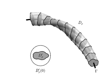
Figure 2.1: Sketch of a thin tubular scattering object $D_{\rho}$ with cross-section $D_{\rho}^{\prime}\subseteq B_{r}^{\prime}(0)$.

Remark 2.1.

The definition (2.6) does not cover thin tubular scattering objects $D_{\rho}$ with closed center curves $K$. However, the results established in the Theorems 3.1 and 4.1 below remain valid in this case, and the proofs can actually be simplified because one does not have to take into account the ends of the tube. $\lozenge$

We suppose that the medium inside the thin tubular scattering object has constant electric permittivity $\varepsilon_{1}>0$ and constant magnetic permeability $\mu_{1}>0$. Accordingly, the permittivity and permeability distributions in the entire domain are given by

$$\varepsilon_{\rho}({\bm{x}})\,:=\,\begin{cases}\varepsilon_{1}\,,&{\bm{x}}\in D_{\rho}\,,\\ \varepsilon_{0}\,,&{\bm{x}}\in{{\mathbb{R}}^{3}}\setminus\overline{D_{\rho}}\,,\end{cases}\qquad\text{and}\qquad\mu_{\rho}({\bm{x}})\,:=\,\begin{cases}\mu_{1}\,,&{\bm{x}}\in D_{\rho}\,,\\ \mu_{0}\,,&{\bm{x}}\in{{\mathbb{R}}^{3}}\setminus\overline{D_{\rho}}\,.\end{cases}$$ (2.7)

We also use the notation $\varepsilon_{r}:=\varepsilon_{1}/\varepsilon_{0}$ and $\mu_{r}:=\mu_{1}/\mu_{0}$ for the relative electric permittivity and the relative magnetic permeability, respectively. The electromagnetic field $({\bm{E}}_{\rho},{\bm{H}}_{\rho})$ in the perturbed medium satisfies

$${\mathbf{curl}}{\bm{E}}_{\rho}-\mathrm{i}\omega\mu_{\rho}{\bm{H}}_{\rho}\,=\,0\,,\quad{\mathbf{curl}}{\bm{H}}_{\rho}+\mathrm{i}\omega\varepsilon_{\rho}{\bm{E}}_{\rho}\,=\,0\qquad\text{in }{{\mathbb{R}}^{3}}\,.$$ (2.8)

Rewriting this total field as a superposition

$$({\bm{E}}_{\rho},{\bm{H}}_{\rho})\,=\,({\bm{E}}^{i},{\bm{H}}^{i})+({\bm{E}}^{s}_{\rho},{\bm{H}}^{s}_{\rho})$$

of the incident field $({\bm{E}}^{i},{\bm{H}}^{i})$ and a scattered field $({\bm{E}}^{s}_{\rho},{\bm{H}}^{s}_{\rho})$, we assume that the scattered field satisfies the Silver-Müller radiation condition

$$\lim_{|{\bm{x}}|\to\infty}(\sqrt{\mu_{0}}{\bm{H}}^{s}_{\rho}({\bm{x}})\times{\bm{x}}-|{\bm{x}}|\sqrt{\varepsilon_{0}}{\bm{E}}^{s}_{\rho}({\bm{x}}))\,=\,0$$ (2.9)

uniformly with respect to all directions $\widehat{{\bm{x}}}:={\bm{x}}/|{\bm{x}}|\in{S^{2}}$.

In the following we will work with the electric field only. Eliminating the magnetic field from the system (2.1) gives

$${\mathbf{curl}}{\mathbf{curl}}{\bm{E}}^{i}-k^{2}{\bm{E}}^{i}\,=\,0\qquad\text{in }{{\mathbb{R}}^{3}}\,,$$ (2.10a)

while (2.8) reduces to

$${\mathbf{curl}}\Bigl{(}\frac{1}{\mu_{\rho}}{\mathbf{curl}}{\bm{E}}_{\rho}\Bigr{)}-\omega^{2}\varepsilon_{\rho}{\bm{E}}_{\rho}\,=\,0\qquad\text{in }{{\mathbb{R}}^{3}}\,,$$ (2.10b)

and (2.9) turns into

$$\lim_{|{\bm{x}}|\to\infty}({\mathbf{curl}}{\bm{E}}^{s}_{\rho}({\bm{x}})\times{\bm{x}}-\mathrm{i}k|{\bm{x}}|{\bm{E}}^{s}_{\rho}({\bm{x}}))\,=\,0\,.$$ (2.10c)

Remark 2.2.

Throughout this work, Maxwell’s equations are always to be understood in weak sense. For instance, ${\bm{E}}_{\rho}\in H_{\mathrm{loc}}({\mathbf{curl}};{{\mathbb{R}}^{3}})$ is a solution to (2.10b) if and only if

$$\int_{{\mathbb{R}}^{3}}\Bigl{(}\frac{1}{\mu_{\rho}}{\mathbf{curl}}{\bm{E}}_{\rho}\cdot{\mathbf{curl}}{\bm{V}}-\omega^{2}\varepsilon_{\rho}{\bm{E}}_{\rho}\cdot{\bm{V}}\Bigr{)}\,\operatorname{d\!}{\bm{x}}\,=\,0\qquad\text{for all }{\bm{V}}\in H_{0}({\mathbf{curl}};{{\mathbb{R}}^{3}})\,.$$

Standard regularity results yield smoothness of ${\bm{E}}_{\rho}$ and ${\bm{E}}^{s}_{\rho}$ in ${{\mathbb{R}}^{3}}\setminus\overline{{B_{R}(0)}}$ for some $R>0$ sufficiently large, and the entire solution ${\bm{E}}^{i}$ is smooth throughout ${{\mathbb{R}}^{3}}$. In particular the Silver-Müller radiation condition (2.10c) is well defined.  $\lozenge$

Lemma 2.3.

Suppose that the incident field ${\bm{E}}^{i}\in H_{\mathrm{loc}}({\mathbf{curl}};{{\mathbb{R}}^{3}})$ satisfies (2.10a). Then there exists a constant $\rho_{0}>0$ depending only on $R$, $\omega$, $\varepsilon_{0}$ and $\mu_{0}$ such that for all $0<\rho<\rho_{0}$ the scattering problem (2.10b)–(2.10c) has a unique solution ${\bm{E}}_{\rho}\in H_{\mathrm{loc}}({\mathbf{curl}};{{\mathbb{R}}^{3}})$. Furthermore, the scattered field ${\bm{E}}^{s}_{\rho}$ has the asymptotic behaviour

$${\bm{E}}^{s}_{\rho}({\bm{x}})\,=\,\frac{e^{\mathrm{i}k|{\bm{x}}|}}{4\pi|{\bm{x}}|}\bigl{(}{\bm{E}}_{\rho}^{\infty}(\widehat{{\bm{x}}})+\mathcal{O}(|{\bm{x}}|^{-1})\bigr{)}\qquad\text{as }|\bf{\bm{x}}|\to\infty$$

uniformly in $\widehat{{\bm{x}}}={\bm{x}}/|{\bm{x}}|$. The vector function ${\bm{E}}^{\infty}_{\rho}$ is called the electric far field pattern.

Proof.

The unique solvability follows, e.g., by combining the arguments in [35, Sec. 10.3] with the uniqueness result [10, Thm. 3.1]. The far field expansion is, e.g., shown in [35, Cor. 9.5]. ∎

3 The asymptotic perturbation formula

We derive an asymptotic perturbation formula for the scattered electric field ${\bm{E}}^{s}_{\rho}$ and the electric far field pattern ${\bm{E}}^{\infty}_{\rho}$ as the radius $\rho$ of the cross-section $D_{\rho}^{\prime}$ of the scattering object $D_{\rho}$ in (2.6) tends to zero relative to the wave length $\lambda=2\pi/k$. Expansions of this type are available in the literature for time-harmonic electromagnetic fields (see, e.g., [1, 8, 9, 28]). However, the existing results for Maxwell’s equations are either formulated on bounded domains, or for scattering problems on unbounded domains but with different geometrical assumptions on the scattering objects than considered in this work. In the following we combine a result for boundary value problems with scatterers of very general geometries from [1, 28] and an integral equation technique developed in [4, 9] to arrive at an asymptotic perturbation formula that applies to our setup.

We consider a sequence of radii $({\rho_{n}})_{n}\subseteq(0,r/2)$ converging to zero, a sequence of measurable cross-sections $D_{\rho_{n}}^{\prime}\subseteq B_{\rho_{n}}^{\prime}(0)$, $n\in{\mathbb{N}}$, and a two-dimensional parameter dependent rotation matrix $R_{\theta}\in C^{1}([-L,L],{\mathbb{R}}^{2\times 2})$ as in (2.3).

Then, as $n\infty$,

$$|D_{\rho_{n}}^{\prime}|^{-1}\chi_{D_{\rho_{n}}^{\prime}}\text{ converges in the sense of measures to }\mu^{\prime}$$ (3.1)

where $\mu^{\prime}$ is the two-dimensional Dirac measure with support in $0$. Recalling (2.2) we denote by $\kappa(s):=|{\bm{p}}_{\Gamma}^{\prime\prime}(s)|$ the curvature of $\Gamma$ and by $\tau(s):=-\frac{\partial{\bm{b}}_{\Gamma}}{\partial s}(s)\cdot{\bm{n}}_{\Gamma}(s)$ the torsion of $\Gamma$ at ${\bm{p}}_{\Gamma}(s)$. A short calculation (see Appendix A) shows that the Jacobian determinant of the local coordinates ${\bm{r}}_{\Gamma}$ from (2.4) is given by

$$J_{\Gamma}(s,\eta,\zeta)\,:=\,\det D{\bm{r}}_{\Gamma}(s,\eta,\zeta)\,=\,1-\kappa{\bm{e}}_{1}^{\prime}\cdot R_{\theta}(s)\begin{bmatrix}\eta\\ \zeta\end{bmatrix}\,,\qquad s\in(-L,L)\,,\;(\eta,\zeta)\in B_{r}^{\prime}(0)\,,$$ (3.2)

where ${\bm{e}}_{1}^{\prime}=(1,0)^{\top}\in{\mathbb{R}}^{2}$. Since $\Gamma$ is a $C^{3}$ curve, we have $\kappa_{\max}:=\|\kappa\|_{C(-L,L)}<\infty$, and it has, e.g., been shown in [33, Thm. 1] that the radius $r>0$ from (2.4) must satisfy $r\kappa_{\max}<1$. In particular, $|J_{\Gamma}|=J_{\Gamma}>0$. Using the notation

$$\nabla_{\eta,\zeta}^{\prime}u\,:=\,\begin{bmatrix}\frac{\partial u}{\partial\eta}&\frac{\partial u}{\partial\zeta}\end{bmatrix}^{\top}\qquad\text{and}\qquad\mathrm{div}_{\eta,\zeta}^{\prime}{\bm{v}}\,:=\,\frac{\partial{\bm{v}}_{\eta}}{\partial\eta}+\frac{\partial{\bm{v}}_{\zeta}}{\partial\zeta}$$

for the two-dimensional gradient and the two-dimensional divergence with respect to $(\eta,\zeta)$, we obtain (see Appendix A for details) that the three-dimensional gradient satisfies, for $s\in(-L,L)$ and $(\eta,\zeta)\in B_{r}^{\prime}(0)$,

$$\nabla u({\bm{r}}_{\Gamma}(s,\eta,\zeta))\\ \,=\,J_{\Gamma}^{-1}(s,\eta,\zeta)\biggl{(}\frac{\partial u}{\partial s}+\Bigl{(}\tau+\frac{\partial\theta}{\partial s}\Bigr{)}(s)\begin{bmatrix}\zeta\\ -\eta\end{bmatrix}\cdot\nabla_{\eta,\zeta}^{\prime}u\biggr{)}{\bm{t}}_{\Gamma}(s)+\begin{bmatrix}{\bm{n}}_{\Gamma}(s)&{\bm{b}}_{\Gamma}(s)\end{bmatrix}R_{\theta}(s)\nabla_{\eta,\zeta}^{\prime}u\,.$$ (3.3)

We note that

$$|D_{\rho_{n}}|\,=\,\int_{-\ell}^{\ell}\int_{D_{\rho_{n}}^{\prime}}J_{\Gamma}(s,\eta,\zeta)\,\operatorname{d\!}(\eta,\zeta)\,\operatorname{d\!}s\,=\,2\ell|D_{\rho_{n}}^{\prime}|\bigl{(}1+\mathcal{O}(\kappa_{\max}{\rho_{n}})\bigr{)}\,,$$

and accordingly we obtain from (3.1) that, for any $\psi\in C(\overline{{B_{R}(0)}})$,

$$\begin{split}\int_{{B_{R}(0)}}\psi\,|D_{\rho_{n}}|^{-1}\chi_{D_{\rho_{n}}}\,\operatorname{d\!}{\bm{x}}&\,=\,\frac{|D_{\rho_{n}}^{\prime}|}{|D_{\rho_{n}}|}\int_{-\ell}^{\ell}\frac{1}{|D_{\rho_{n}}^{\prime}|}\int_{B_{r}^{\prime}(0)}\chi_{D_{\rho_{n}}^{\prime}}(\eta,\zeta)\psi({\bm{r}}_{\Gamma}(s,\eta,\zeta))J_{\Gamma}(s,\eta,\zeta)\,\operatorname{d\!}(\eta,\zeta)\,\operatorname{d\!}s\\ &\to\frac{1}{2\ell}\int_{-\ell}^{\ell}\int_{B_{r}^{\prime}(0)}\psi({\bm{r}}_{\Gamma}(s,\eta,\zeta))\,\operatorname{d\!}\mu^{\prime}\,\operatorname{d\!}s\,=\,\frac{1}{2\ell}\int_{-\ell}^{\ell}\psi({\bm{p}}_{\Gamma}(s))\,\operatorname{d\!}s\end{split}$$

as $n\to\infty$. This means that

$$|D_{\rho_{n}}|^{-1}\chi_{D_{\rho_{n}}}\text{ converges in the sense of measures to }\mu\text{ as }n\to\infty\,,$$ (3.4)

where $\mu$ is the Borel measure given by

$$\int_{{B_{R}(0)}}\psi\,\operatorname{d\!}\mu\,=\,\frac{1}{2\ell}\int_{K}\psi\,\operatorname{d\!}s\qquad\text{for any $\psi\in C(\overline{{B_{R}(0)}})$}\,.$$ (3.5)

The following theorem describes the asymptotic behavior of the scattered electric field ${\bm{E}}^{s}_{\rho_{n}}$ and of the electric far field pattern ${\bm{E}}^{\infty}_{\rho_{n}}$ as the radius ${\rho_{n}}$ of the scattering object $D_{\rho_{n}}$ tends to zero. The matrix function

$$\mathbb{G}({\bm{x}},{\bm{y}})\,:=\,\Phi_{k}({\bm{x}}-{\bm{y}})\mathbb{I}_{3}+\frac{1}{k^{2}}\nabla_{\bm{x}}\mathrm{div}_{\bm{x}}(\Phi_{k}({\bm{x}}-{\bm{y}})\mathbb{I}_{3})\,,\qquad{\bm{x}}\not={\bm{y}}\,,$$

where $\mathbb{I}_{3}\in{{\mathbb{R}}^{3}}$ is the identity matrix and $\Phi_{k}({\bm{x}}-{\bm{y}}):=e^{\mathrm{i}k|{\bm{x}}-{\bm{y}}|}/(4\pi|{\bm{x}}-{\bm{y}}|)$ denotes the fundamental solution of the Helmholtz equation, is called the dyadic Green’s function for Maxwell’s equations (see, e.g., [35, p. 303]).

Theorem 3.1.

Let $K\Subset{B_{R}(0)}$ be a simple $C^{3}$ center curve, and let $r>0$ such that the local parametrization in (2.4) is well defined. Let $({\rho_{n}})_{n}\subseteq(0,r/2)$ be a sequence of radii converging to zero, and let $(D_{\rho_{n}}^{\prime})_{n}$ be a sequence of measurable cross-sections with $D_{\rho_{n}}^{\prime}\subseteq B_{\rho_{n}}^{\prime}(0)$ for all $n\in{\mathbb{N}}$. Suppose that $(D_{\rho_{n}})_{n}\subseteq{B_{R}(0)}$ is the corresponding sequence of thin tubular scattering objects as in (2.6), where the cross-section twists along the center curve subject to a parameter dependent rotation matrix $R_{\theta}\in C^{1}([-L,L],{\mathbb{R}}^{2\times 2})$. Denoting by $(\varepsilon_{{\rho_{n}}})_{n}$ and $(\mu_{{\rho_{n}}})_{n}$ permittivity and permeability distributions as in (2.7), let ${\bm{E}}^{s}_{\rho_{n}}$ be the associated scattered electric field solving (2.10) for some incident electric field ${\bm{E}}^{i}$. Then there exists a subsequence, also denoted by $(D_{\rho_{n}})_{n}$, and matrix valued functions $\mathbb{M}^{\varepsilon},\mathbb{M}^{\mu}\in L^{2}(K,{{\mathbb{R}}^{3\times 3}})$ called electric and magnetic polarization tensors, respectively, such that

$${\bm{E}}^{s}_{\rho_{n}}({\bm{x}})\,=\,\frac{|D_{\rho_{n}}|}{2\ell}\biggl{(}\int_{K}(\mu_{r}-1){\mathbf{curl}}_{x}\mathbb{G}({\bm{x}},{\bm{y}})\mathbb{M}^{\mu}({\bm{y}}){\mathbf{curl}}{\bm{E}}^{i}({\bm{y}})\,\operatorname{d\!}s({\bm{y}})\\ +\int_{K}k^{2}(\varepsilon_{r}-1)\mathbb{G}({\bm{x}},{\bm{y}})\mathbb{M}^{\varepsilon}({\bm{y}}){\bm{E}}^{i}({\bm{y}})\,\operatorname{d\!}s({\bm{y}})\biggr{)}+o(|D_{\rho_{n}}|)\,,\qquad{\bm{x}}\in{{\mathbb{R}}^{3}}\setminus\overline{{B_{R}(0)}}\,.$$ (3.6)

Furthermore, the electric far field pattern satisfies

$${\bm{E}}^{\infty}_{\rho_{n}}(\widehat{{\bm{x}}})\,=\,\frac{|D_{\rho_{n}}|}{2\ell}\biggl{(}\int_{K}(\mu_{r}-1)\mathrm{i}ke^{-\mathrm{i}k\widehat{{\bm{x}}}\cdot{\bm{y}}}(\widehat{{\bm{x}}}\times\mathbb{I}_{3})\mathbb{M}^{\mu}({\bm{y}}){\mathbf{curl}}{\bm{E}}^{i}({\bm{y}})\,\operatorname{d\!}s({\bm{y}})\\ +\int_{K}k^{2}(\varepsilon_{r}-1)e^{-\mathrm{i}k\widehat{{\bm{x}}}\cdot{\bm{y}}}\bigl{(}\widehat{{\bm{x}}}\times(\mathbb{I}_{3}\times\widehat{{\bm{x}}})\bigr{)}\mathbb{M}^{\varepsilon}({\bm{y}}){\bm{E}}^{i}({\bm{y}})\,\operatorname{d\!}s({\bm{y}})\biggr{)}+o(|D_{\rho_{n}}|)\,,\qquad\widehat{{\bm{x}}}\in{S^{2}}\,.$$ (3.7)

The subsequence $(D_{\rho_{n}})_{n}$ and the polarization tensors $\mathbb{M}^{\varepsilon}$ and $\mathbb{M}^{\mu}$ are independent of the incident electric field ${\bm{E}}^{i}$. The terms $o(|D_{\rho_{n}}|)$ in (3.6) and (3.7) are such that $\|o(|D_{\rho_{n}}|)\|_{L^{\infty}(\partial{B_{R}(0)})}/|D_{\rho_{n}}|$ and $\|o(|D_{\rho_{n}}|)\|_{L^{\infty}({S^{2}})}/|D_{\rho_{n}}|$ converge to zero uniformly for all ${\bm{E}}^{i}$ satisfying $\|{\bm{E}}^{i}\|_{H({\mathbf{curl}};{B_{R}(0)})}\leq C$ for some fixed $C>0$.

Proof.

An analysis similar to [9, 4], using the asymptotic perturbation formula for the Maxwell boundary value problem from [1, 28] instead of [8], and applying (3.5) gives the result. ∎

All components of the leading order terms in the asymptotic representation formulas (3.6) and (3.7), except for the polarization tensors $\mathbb{M}^{\varepsilon},\mathbb{M}^{\mu}\in L^{2}(K,{{\mathbb{R}}^{3\times 3}})$, are either known explicitly or can be evaluated straightforwardly. The polarization tensors are defined as follows (see [18, 21, 28]). Let $\gamma\in\{\varepsilon,\mu\}$. For ${\bm{\xi}}\in{S^{2}}$ and $n\in{\mathbb{N}}$ let $W^{({\bm{\xi}})}_{{\rho_{n}}}\in H^{1}_{0}({B_{R}(0)})$ be the corrector potentials satisfying

$$\mathrm{div}\bigl{(}\gamma_{{\rho_{n}}}\nabla W^{({\bm{\xi}})}_{{\rho_{n}}}\bigr{)}\,=\,-\mathrm{div}\bigl{(}(\gamma_{{\rho_{n}}}-\gamma_{0}){\bm{\xi}}\bigr{)}\quad\text{in ${B_{R}(0)}$}\,,\qquad W^{({\bm{\xi}})}_{{\rho_{n}}}\,=\,0\quad\text{on $\partial{B_{R}(0)}$}\,.$$ (3.8)

Then, considering the subsequence $(D_{\rho_{n}})_{n}$ from Theorem 3.1, the polarization tensor $\mathbb{M}^{\gamma}$ is uniquely determined by

$$\frac{1}{2\ell}\int_{K}{\bm{\xi}}\cdot\mathbb{M}^{\gamma}{\bm{\xi}}\psi\,\operatorname{d\!}s\,=\,\frac{1}{|D_{\rho_{n}}|}\int_{D_{\rho_{n}}}|{\bm{\xi}}|^{2}\psi\,\operatorname{d\!}{\bm{x}}+\frac{1}{|D_{\rho_{n}}|}\int_{D_{\rho_{n}}}\bigl{(}{\bm{\xi}}\cdot\nabla W^{({\bm{\xi}})}_{{\rho_{n}}}\bigr{)}\psi\,\operatorname{d\!}{\bm{x}}+o(1)$$ (3.9)

for all $\psi\in C(\overline{{B_{R}(0)}})$ and any ${\bm{\xi}}\in{S^{2}}$. Similar notions of polarization tensors appear in various contexts. The term was introduced by Polya, Schiffer and Szegö [39, 40], and they have been widely studied in the theory of homogenization as the low volume fraction limit of the effective properties of the dilute two phase composites (see, e.g., [32, 34, 36]). For the specific form considered here, it has been shown in [18, 21] that the values of the functions $\mathbb{M}^{\gamma}$ are symmetric and positive definite in the sense that

$$\mathbb{M}^{\gamma}_{ij}({\bm{x}})\,=\,\mathbb{M}^{\gamma}_{ji}({\bm{x}})\qquad\text{for $1\leq i,j\leq 3$ and a.e.\ }{\bm{x}}\in K\,,$$ (3.10)

and

$$\min\Bigl{\{}1,\frac{\gamma_{0}({\bm{x}})}{\gamma_{1}({\bm{x}})}\Bigr{\}}\,\leq\,{\bm{\xi}}\cdot\mathbb{M}^{\gamma}({\bm{x}}){\bm{\xi}}\,\leq\,\max\Bigl{\{}1,\frac{\gamma_{0}({\bm{x}})}{\gamma_{1}({\bm{x}})}\Bigr{\}}\qquad\text{for every ${\bm{\xi}}\in{S^{2}}$ and a.e.\ ${\bm{x}}\in K$}\,.$$ (3.11)

Analytic expressions for $\mathbb{M}^{\gamma}$ have been derived for several basic geometries such as, e.g., when $(D_{\rho_{n}})_{n}$ is a family of diametrically small ellipsoids (see [6]), a family of thin neighborhoods of a hypersurface (see [15]), or a family of thin neighborhoods of a straight line segment (see [13]). In the next section we extend the result from [13] to thin neighborhoods of smooth curves of $(D_{\rho_{n}})_{n}$ as in (2.6), and we derive a spectral representation of the polarization tensor in terms of the center curve $K$ and the two-dimensional polarization tensor of the cross-sections $(D_{\rho_{n}}^{\prime})_{n}$. In [13, 23, 29], the authors expressed interest such a characterization of the polarisation tensor for thin tubular objects for various applications. Therewith, the leading order terms in the asymptotic representation formulas (3.6) and (3.7) can be evaluated very efficiently.

Remark 3.2.

The characterization of the polarization tensor $\mathbb{M}^{\gamma}\in L^{2}(K;{{\mathbb{R}}^{3\times 3}})$ in (3.9) remains valid when the domain ${B_{R}(0)}$ in (3.8) is replaced by ${\Omega_{r}}$ from (2.5) (see [21, Rem. 1]). The regularity results that are used in the proof of [21, Lmm. 1] are applicable because ${\Omega_{r}}$ is $C^{2}$ away from the ends of the tube and convex in a neighborhood of the ends of the tube. This will be used in Section 4 below. $\lozenge$

4 The polarization tensor of a thin tubular scattering object

Let $\gamma\in\{\varepsilon,\mu\}$. We assign a two-dimensional polarization tensor ${m^{\gamma}\in{\mathbb{R}}^{2\times 2}}$ to the sequence of cross-sections $(D_{\rho_{n}}^{\prime})_{n}$ of the scattering objects $(D_{\rho_{n}})_{n}$ as follows. Let

$$\gamma_{{\rho_{n}}}^{\prime}(\eta,\zeta)\,:=\,\begin{cases}\gamma_{1}\,,&(\eta,\zeta)\in D_{\rho_{n}}^{\prime}\,,\\ \gamma_{0}\,,&(\eta,\zeta)\in B_{r}^{\prime}(0)\setminus\overline{D_{\rho_{n}}^{\prime}}\,,\end{cases}$$

i.e., $\gamma_{{\rho_{n}}}^{\prime}$ is just the electric permittivity or the magnetic permeability distribution associated to the cross-section $D_{\rho_{n}}^{\prime}$. For each ${\bm{\xi}}^{\prime}\in{S^{1}}$ we denote by $w^{({\bm{\xi}}^{\prime})}_{{\rho_{n}}}\in H^{1}_{0}(B_{r}^{\prime}(0))$ the unique solution to

$$\mathrm{div}_{\eta,\zeta}^{\prime}\bigl{(}\gamma_{{\rho_{n}}}^{\prime}\nabla_{\eta,\zeta}^{\prime}w^{({\bm{\xi}}^{\prime})}_{{\rho_{n}}}\bigr{)} \,=\,-\mathrm{div}_{\eta,\zeta}^{\prime}\bigl{(}(\gamma_{1}-\gamma_{0})\chi_{D_{\rho_{n}}^{\prime}}{\bm{\xi}}^{\prime}\bigr{)} \text{in $B_{r}^{\prime}(0)$}\,,$$ (4.1a)

$$w^{({\bm{\xi}}^{\prime})}_{{\rho_{n}}} \,=\,0 \text{on $\partial B_{r}^{\prime}(0)$}\,,$$ (4.1b)

and accordingly we define $m^{\gamma}\in{\mathbb{R}}^{2\times 2}$ (possibly up to extraction of a subsequence) by

$${\bm{\xi}}^{\prime}\cdot m^{\gamma}{\bm{\xi}}^{\prime}\,\psi(0)\,=\,\frac{1}{|D_{\rho_{n}}^{\prime}|}\int_{D_{\rho_{n}}^{\prime}}|{\bm{\xi}}^{\prime}|^{2}\psi\,\operatorname{d\!}{\bm{x}}^{\prime}+\frac{1}{|D_{\rho_{n}}^{\prime}|}\int_{D_{\rho_{n}}^{\prime}}\bigl{(}{\bm{\xi}}^{\prime}\cdot\nabla_{\eta,\zeta}^{\prime}w^{({\bm{\xi}}^{\prime})}_{{\rho_{n}}}\bigr{)}\psi\,\operatorname{d\!}{\bm{x}}^{\prime}+o(1)$$ (4.2)

for all $\psi\in C(\overline{B_{r}^{\prime}(0)})$ and any ${\bm{\xi}}^{\prime}\in{S^{1}}$.

The following theorem is the main result of this section.

Theorem 4.1.

Let $K\Subset{B_{R}(0)}$ be a simple $C^{3}$ center curve, and let $r>0$ such that the local parametrization in (2.4) is well defined. Let $({\rho_{n}})_{n}\subseteq(0,r/2)$ be a sequence of radii converging to zero, and let $(D_{\rho_{n}}^{\prime})_{n}$ be a sequence of measurable cross-sections with $D_{\rho_{n}}^{\prime}\subseteq B_{\rho_{n}}^{\prime}(0)$ for all $n\in{\mathbb{N}}$. Suppose that $(D_{\rho_{n}})_{n}\subseteq{B_{R}(0)}$ is the corresponding sequence of thin tubular scattering objects as in (2.6), where the cross-section twists along the center curve subject to a parameter dependent rotation matrix $R_{\theta}\in C^{1}([-L,L],{\mathbb{R}}^{2\times 2})$. Denoting by $(\gamma_{{\rho_{n}}})_{n}$ a parameter distribution as in (2.7), let $\mathbb{M}^{\gamma}$ be the polarization tensor corresponding to the thin tubular scattering objects $(D_{\rho_{n}})_{n}$ from (3.9) (defined possibly up to extraction of a subsequence). Denoting by $m^{\gamma}$ the polarization tensor corresponding to the cross-sections $(D_{\rho_{n}}^{\prime})_{n}$ from (4.2) (defined possibly up to extraction of a subsequence), the following pointwise characterization of $\mathbb{M}^{\gamma}$ holds for a.e. $s\in(-\ell,\ell)$:

1. The unit tangent vector ${\bm{t}}_{\Gamma}(s)$ is an eigenvector of the matrix $\mathbb{M}^{\gamma}({\bm{p}}_{\Gamma}(s))$ corresponding to the eigenvalue $1$, i.e.,

   $${\bm{t}}_{\Gamma}(s)\cdot\mathbb{M}^{\gamma}({\bm{p}}_{\Gamma}(s)){\bm{t}}_{\Gamma}(s)\,=\,1\qquad\text{for a.e.\ $s\in(-\ell,\ell)$}\,.$$ (4.3)

2. Let ${\bm{\xi}}^{\prime}\in{S^{1}}$, and let ${\bm{\xi}}\in C^{1}(K,{S^{2}})$ be given by ${\bm{\xi}}(s):=\begin{bmatrix}{\bm{n}}_{\Gamma}(s)&{\bm{b}}_{\Gamma}(s)\end{bmatrix}{\bm{\xi}}^{\prime}\in{S^{2}}$ for all ${s\in(-\ell,\ell)}$. Then,

   $${\bm{\xi}}(s)\cdot\mathbb{M}^{\gamma}({\bm{p}}_{\Gamma}(s)){\bm{\xi}}(s)\,=\,{\bm{\xi}}^{\prime}\cdot\bigl{(}R_{\theta}(s)m^{\gamma}R_{\theta}^{-1}(s)\bigr{)}{\bm{\xi}}^{\prime}\qquad\text{for a.e.\ $s\in(-\ell,\ell)$}\,.$$ (4.4)

Since the polarization tensor $\mathbb{M}^{\gamma}({\bm{p}}_{\Gamma}(s))$ is symmetric, the first part of the theorem implies that there are two more eigenvalues in the plane orthogonal to ${\bm{t}}_{\Gamma}(s)$, which is spanned by ${\bm{n}}_{\Gamma}(s)$ and ${\bm{b}}_{\Gamma}(s)$. The second part of the theorem says that in this plane the polarization tensor $\mathbb{M}^{\gamma}({\bm{p}}_{\Gamma}(s))$ coincides with the polarization tensor $R_{\theta}(s)m^{\gamma}R_{\theta}^{-1}(s)$ of the twisted two-dimensional cross-sections.

The proof of Theorem 4.1 relies on the following proposition, which extends the characterization of the polarization tensor $\mathbb{M}^{\gamma}$ in (3.9) from constant vectors ${\bm{\xi}}\in{S^{2}}$ to vector-valued functions ${\bm{\xi}}\in C^{1}({\Omega_{r}},{S^{2}})$.

Proposition 4.2.

Let ${\bm{\xi}}\in C^{1}({\Omega_{r}},{S^{2}})$, and denote by $W^{({\bm{\xi}})}_{{\rho_{n}}}\in H^{1}_{0}({\Omega_{r}})$ the corresponding solution to (3.8). Then the polarization tensor $\mathbb{M}^{\gamma}$ satisfies

$$\frac{1}{2\ell}\int_{K}{\bm{\xi}}\cdot\mathbb{M}^{\gamma}{\bm{\xi}}\psi\,\operatorname{d\!}s\,=\,\frac{1}{|D_{\rho_{n}}|}\int_{D_{\rho_{n}}}|{\bm{\xi}}|^{2}\psi\,\operatorname{d\!}{\bm{x}}+\frac{1}{|D_{\rho_{n}}|}\int_{D_{\rho_{n}}}\bigl{(}{\bm{\xi}}\cdot\nabla W^{({\bm{\xi}})}_{{\rho_{n}}}\bigr{)}\psi\,\operatorname{d\!}{\bm{x}}+o(1)$$

for all $\psi\in C(\overline{{\Omega_{r}}})$.

Proof.

We denote by $({\bm{e}}_{1},{\bm{e}}_{2},{\bm{e}}_{3})$ the standard basis of ${{\mathbb{R}}^{3}}$, and we consider ${\bm{\xi}}=\sum_{i=1}^{3}\xi_{i}{\bm{e}}_{i}\in C^{1}({\Omega_{r}},{S^{2}})$. Let $W^{({\bm{\xi}})}_{{\rho_{n}}}\in H^{1}_{0}({\Omega_{r}})$ be the corresponding solutions to (3.8), and let $W_{{\rho_{n}}}^{(e_{j})}$, $1\leq j\leq 3$, be the solutions to (3.8) with ${\bm{\xi}}={\bm{e}}_{j}$. Then, using (3.9) we find that

$$\begin{split}&\frac{1}{2\ell}\int_{K}{\bm{\xi}}({\bm{x}})\cdot\mathbb{M}^{\gamma}({\bm{x}}){\bm{\xi}}({\bm{x}})\psi({\bm{x}})\,\operatorname{d\!}s({\bm{x}})\,=\,\sum_{i,j=1}^{3}\frac{1}{2\ell}\int_{K}{\bm{e}}_{i}\cdot\mathbb{M}^{\gamma}({\bm{x}}){\bm{e}}_{j}\bigl{(}\xi_{i}\xi_{j}\psi\bigr{)}({\bm{x}})\,\operatorname{d\!}s({\bm{x}})\\ &\,=\,\sum_{i,j=1}^{3}\frac{1}{|D_{\rho_{n}}|}\int_{D_{\rho_{n}}}{\bm{e}}_{i}\cdot{\bm{e}}_{j}\bigl{(}\xi_{i}\xi_{j}\psi\bigr{)}({\bm{x}})\,\operatorname{d\!}{\bm{x}}+\sum_{i,j=1}^{3}\frac{1}{|D_{\rho_{n}}|}\int_{D_{\rho_{n}}}{\bm{e}}_{i}\cdot\nabla W_{{\rho_{n}}}^{(e_{j})}({\bm{x}})\bigl{(}\xi_{i}\xi_{j}\psi\bigr{)}({\bm{x}})\,\operatorname{d\!}{\bm{x}}+o(1)\\ &\,=\,\frac{1}{|D_{\rho_{n}}|}\int_{D_{\rho_{n}}}|{\bm{\xi}}({\bm{x}})|^{2}\psi({\bm{x}})\,\operatorname{d\!}{\bm{x}}+\frac{1}{|D_{\rho_{n}}|}\int_{D_{\rho_{n}}}{\bm{\xi}}({\bm{x}})\cdot\nabla W^{({\bm{\xi}})}_{{\rho_{n}}}({\bm{x}})\psi({\bm{x}})\,\operatorname{d\!}{\bm{x}}\\ &\phantom{\,=\,}-\frac{1}{|D_{\rho_{n}}|}\int_{D_{\rho_{n}}}{\bm{\xi}}({\bm{x}})\cdot\Bigl{(}\nabla W^{({\bm{\xi}})}_{{\rho_{n}}}-\sum_{j=1}^{3}\xi_{j}\nabla W_{{\rho_{n}}}^{(e_{j})}\Bigr{)}({\bm{x}})\psi({\bm{x}})\,\operatorname{d\!}{\bm{x}}+o(1)\,.\end{split}$$

Applying Hölder’s inequality gives

$$\biggl{|}\int_{D_{\rho_{n}}}{\bm{\xi}}\cdot\Bigl{(}\nabla W^{({\bm{\xi}})}_{{\rho_{n}}}-\sum_{j=1}^{3}\xi_{j}\nabla W_{{\rho_{n}}}^{(e_{j})}\Bigr{)}\psi\,\operatorname{d\!}{\bm{x}}\biggr{|}\,\leq\,C|D_{\rho_{n}}|^{\frac{1}{2}}\Bigl{\|}\nabla W^{({\bm{\xi}})}_{{\rho_{n}}}-\sum_{j=1}^{3}\xi_{j}\nabla W_{{\rho_{n}}}^{(e_{j})}\Bigr{\|}_{L^{2}({\Omega_{r}})}\,.$$ (4.5)

To finish the proof, we show that the right hand side of (4.5) is $o(|D_{\rho_{n}}|)$ as $n\to\infty$.

We note that (3.8) gives

$$\begin{split}\mathrm{div}\Bigl{(}\gamma_{{\rho_{n}}}\nabla\Bigl{(}W^{({\bm{\xi}})}_{{\rho_{n}}}-\sum_{j=1}^{3}\xi_{j}W_{{\rho_{n}}}^{(e_{j})}\Bigr{)}\Bigr{)}&\,=\,-\mathrm{div}\bigl{(}(\gamma_{{\rho_{n}}}-\gamma_{0}){\bm{\xi}}\bigr{)}\\ &\phantom{\,=\,}-\sum_{j=1}^{3}\mathrm{div}\bigl{(}\bigl{(}\gamma_{{\rho_{n}}}\nabla W_{{\rho_{n}}}^{(e_{j})}\bigr{)}\xi_{j}\bigr{)}-\sum_{j=1}^{3}\mathrm{div}\bigl{(}\gamma_{{\rho_{n}}}W_{{\rho_{n}}}^{(e_{j})}\nabla\xi_{j}\bigr{)}\,.\end{split}$$

Furthermore,

$$\begin{split}\sum_{j=1}^{3}\mathrm{div}\bigl{(}\bigl{(}\gamma_{{\rho_{n}}}\nabla W_{{\rho_{n}}}^{(e_{j})}\bigr{)}\xi_{j}\bigr{)}&\,=\,-\sum_{j=1}^{3}\mathrm{div}\bigl{(}(\gamma_{{\rho_{n}}}-\gamma_{0}){\bm{e}}_{j}\bigr{)}\xi_{j}+\sum_{j=1}^{3}\gamma_{{\rho_{n}}}\nabla W_{{\rho_{n}}}^{(e_{j})}\cdot\nabla\xi_{j}\,,\end{split}$$

and rewriting ${\bm{\xi}}=\sum_{j=1}^{3}\xi_{j}{\bm{e}}_{j}$ we obtain that

$$\mathrm{div}\bigl{(}(\gamma_{{\rho_{n}}}-\gamma_{0}){\bm{\xi}}\bigr{)}\,=\,\sum_{j=1}^{3}\mathrm{div}\bigl{(}(\gamma_{{\rho_{n}}}-\gamma_{0}){\bm{e}}_{j}\bigr{)}\xi_{j}+\sum_{j=1}^{3}(\gamma_{{\rho_{n}}}-\gamma_{0}){\bm{e}}_{j}\cdot\nabla\xi_{j}\,.$$

Accordingly, $W^{({\bm{\xi}})}_{{\rho_{n}}}-\sum_{j=1}^{3}\xi_{j}W_{{\rho_{n}}}^{(e_{j})}\in H^{1}_{0}({\Omega_{r}})$ satisfies

$$\begin{split}\mathrm{div}\Bigl{(}\gamma_{{\rho_{n}}}\nabla\Bigl{(}W^{({\bm{\xi}})}_{{\rho_{n}}}-\sum_{j=1}^{3}\xi_{j}W_{{\rho_{n}}}^{(e_{j})}\Bigr{)}\Bigr{)}&\,=\,-\sum_{j=1}^{3}(\gamma_{{\rho_{n}}}-\gamma_{0}){\bm{e}}_{j}\cdot\nabla\xi_{j}-\sum_{j=1}^{3}\gamma_{{\rho_{n}}}\nabla W_{{\rho_{n}}}^{(e_{j})}\cdot\nabla\xi_{j}\\ &\phantom{\,=\,}-\sum_{j=1}^{3}\mathrm{div}\bigl{(}\gamma_{{\rho_{n}}}W_{{\rho_{n}}}^{(e_{j})}\nabla\xi_{j}\bigr{)}\,.\end{split}$$

Now let $r_{\rho_{n}}^{(1)},r_{\rho_{n}}^{(2)},r_{\rho_{n}}^{(3)}\in H^{1}_{0}({\Omega_{r}})$ be the unique solutions to

$$\mathrm{div}(\gamma_{{\rho_{n}}}\nabla r_{\rho_{n}}^{(1)}) \,=\,-\sum_{j=1}^{3}\mathrm{div}(\gamma_{{\rho_{n}}}W_{{\rho_{n}}}^{(e_{j})}\nabla\xi_{j}) \text{in ${\Omega_{r}}$}\,,\qquad r_{\rho_{n}}^{(1)}\,=\,0\qquad\text{on $\partial{\Omega_{r}}$}\,,$$ (4.6a)

$$\mathrm{div}(\gamma_{{\rho_{n}}}\nabla r_{\rho_{n}}^{(2)}) \,=\,-\sum_{j=1}^{3}\gamma_{{\rho_{n}}}\nabla W_{{\rho_{n}}}^{(e_{j})}\cdot\nabla\xi_{j} \text{in ${\Omega_{r}}$}\,,\qquad r_{\rho_{n}}^{(2)}\,=\,0\qquad\text{on $\partial{\Omega_{r}}$}\,,$$ (4.6b)

$$\mathrm{div}(\gamma_{{\rho_{n}}}\nabla r_{\rho_{n}}^{(3)}) \,=\,-\sum_{j=1}^{3}(\gamma_{{\rho_{n}}}-\gamma_{0})({\bm{e}}_{j}\cdot\nabla\xi_{j}) \text{in ${\Omega_{r}}$}\,,\qquad r_{\rho_{n}}^{(3)}\,=\,0\qquad\text{on $\partial{\Omega_{r}}$}\,.$$ (4.6c)

The uniqueness of solutions to the Dirichlet problem implies that

$$W^{({\bm{\xi}})}_{{\rho_{n}}}-\sum_{j=1}^{3}\xi_{j}W_{{\rho_{n}}}^{(e_{j})}\,=\,r_{\rho_{n}}^{(1)}+r_{\rho_{n}}^{(2)}+r_{\rho_{n}}^{(3)}\,,$$

and we have the following estimates for $r_{\rho_{n}}^{(1)},r_{\rho_{n}}^{(2)}$, and $r_{\rho_{n}}^{(3)}$. Using the well-posedness of (4.6a) and (B.2b) we find that

$$\begin{split}\|r_{\rho_{n}}^{(1)}\|_{H^{1}({\Omega_{r}})}&\,\leq\,C\Bigl{\|}\sum_{j=1}^{3}\gamma_{{\rho_{n}}}W_{{\rho_{n}}}^{(e_{j})}\nabla\xi_{j}\Bigr{\|}_{L^{2}({\Omega_{r}})}\,\leq\,C\max_{j}\|\nabla\xi_{j}\|_{L^{\infty}({\Omega_{r}})}\|W_{{\rho_{n}}}^{(e_{j})}\|_{L^{2}({\Omega_{r}})}\\ &\,\leq\,C\|{\bm{\xi}}\|_{C^{1}({\Omega_{r}})}|D_{\rho_{n}}|^{\frac{3}{4}}\,.\end{split}$$

Similarly, using Poincare’s inequality, the weak formulation of (4.6b), Hölder’s inequality, Sobolev’s embedding theorem (see, e.g., [26, p. 158]), and (B.2c) we obtain that

$$\begin{split}&\|r_{\rho_{n}}^{(2)}\|_{H^{1}({\Omega_{r}})}^{2}\,\leq\,C\Bigl{|}\int_{\Omega_{r}}\gamma_{{\rho_{n}}}\nabla r_{\rho_{n}}^{(2)}\cdot\nabla r_{\rho_{n}}^{(2)}\,\operatorname{d\!}{\bm{x}}\Bigr{|}\,=\,C\Bigl{|}\int_{\Omega_{r}}\sum_{j=1}^{3}\gamma_{{\rho_{n}}}\bigl{(}\nabla W_{{\rho_{n}}}^{(e_{j})}\cdot\nabla\xi_{j}\bigr{)}r_{\rho_{n}}^{(2)}\,\operatorname{d\!}{\bm{x}}\Bigr{|}\\ &\,\leq\,C\Bigl{\|}\sum_{j=1}^{3}\gamma_{{\rho_{n}}}\nabla W_{{\rho_{n}}}^{(e_{j})}\Bigr{\|}_{L^{\frac{6}{5}}({\Omega_{r}})}\max_{j}\|\nabla\xi_{j}\|_{L^{\infty}({\Omega_{r}})}\|r_{\rho_{n}}^{(2)}\|_{L^{6}({\Omega_{r}})}\\ &\,\leq\,C|D_{\rho_{n}}|^{\frac{5}{6}}\|{\bm{\xi}}\|_{C^{1}({\Omega_{r}})}\|\nabla r_{\rho_{n}}^{(2)}\|_{L^{2}({\Omega_{r}})}\,\leq\,C|D_{\rho_{n}}|^{\frac{5}{6}}\|{\bm{\xi}}\|_{C^{1}({\Omega_{r}})}\|r_{\rho_{n}}^{(2)}\|_{H^{1}({\Omega_{r}})}\,.\end{split}$$

For the third term $r_{\rho_{n}}^{(3)}$ we note that, using Poincare’s inequality, the weak formulation of (4.6c), Hölder’s inequality, and Sobolev’s embedding theorem,

$$\begin{split}\|r_{\rho_{n}}^{(3)}\|_{H^{1}({\Omega_{r}})}^{2}&\,\leq\,C\Bigl{|}\int_{\Omega_{r}}\gamma_{{\rho_{n}}}\nabla r_{\rho_{n}}^{(3)}\cdot\nabla r_{\rho_{n}}^{(3)}\,\operatorname{d\!}{\bm{x}}\Bigr{|}\,=\,C\Bigl{|}\int_{\Omega_{r}}(\gamma_{{\rho_{n}}}-\gamma_{0})\sum_{j=1}^{3}({\bm{e}}_{j}\cdot\nabla\xi_{j})r_{\rho_{n}}^{(3)}\,\operatorname{d\!}{\bm{x}}\Bigr{|}\\ &\,\leq\,C\|\gamma_{{\rho_{n}}}-\gamma_{0}\|_{L^{\frac{6}{5}}({\Omega_{r}})}\max_{j}\|\nabla\xi_{j}\|_{L^{\infty}({\Omega_{r}})}\|r_{\rho_{n}}^{(3)}\|_{L^{6}({\Omega_{r}})}\\ &\,\leq\,C|D_{\rho_{n}}|^{\frac{5}{6}}\|{\bm{\xi}}\|_{C^{1}({\Omega_{r}})}\|\nabla r_{\rho_{n}}^{(3)}\|_{L^{2}({\Omega_{r}})}\,\leq\,C|D_{\rho_{n}}|^{\frac{5}{6}}\|{\bm{\xi}}\|_{C^{1}({\Omega_{r}})}\|r_{\rho_{n}}^{(3)}\|_{H^{1}({\Omega_{r}})}\,.\end{split}$$

Accordingly,

$$\Bigl{\|}W^{({\bm{\xi}})}_{{\rho_{n}}}-\sum_{j=1}^{3}\xi_{j}W_{{\rho_{n}}}^{(e_{j})}\Bigr{\|}_{H^{1}({\Omega_{r}})}\,\leq\,C\|{\bm{\xi}}\|_{C^{1}({\Omega_{r}})}|D_{\rho_{n}}|^{\frac{3}{4}}\,,$$

and, using (B.2b),

$$\Bigl{\|}\nabla W^{({\bm{\xi}})}_{{\rho_{n}}}-\sum_{j=1}^{3}\xi_{j}\nabla W_{{\rho_{n}}}^{(e_{j})}\Bigr{\|}_{L^{2}({\Omega_{r}})}\,\leq\,\Bigl{\|}\nabla W^{({\bm{\xi}})}_{{\rho_{n}}}-\nabla\Bigl{(}\sum_{j=1}^{3}\xi_{j}W_{{\rho_{n}}}^{(e_{j})}\Bigr{)}\Bigr{\|}_{L^{2}({\Omega_{r}})}+\Bigl{\|}\sum_{j=1}^{3}W_{{\rho_{n}}}^{(e_{j})}\nabla\xi_{j}\Bigr{\|}_{L^{2}({\Omega_{r}})}\\ \,\leq\,C\|{\bm{\xi}}\|_{C^{1}({\Omega_{r}})}|D_{\rho_{n}}|^{\frac{3}{4}}+\|W_{{\rho_{n}}}^{(e_{j})}\|_{L^{2}({\Omega_{r}})}\max_{j}\|\nabla\xi_{j}\|_{L^{\infty}({\Omega_{r}})}\,\leq\,C\|{\bm{\xi}}\|_{C^{1}({\Omega_{r}})}|D_{\rho_{n}}|^{\frac{3}{4}}\,.$$

∎

Next we prove the first part of Theorem 4.1.

Proof of Theorem 4.1(a).

Let ${\bm{\xi}}\in C^{1}({\Omega_{r}})$ be defined by ${\bm{\xi}}({\bm{x}}):={\bm{t}}_{\Gamma}(s)$ for any ${\bm{x}}={\bm{r}}_{\Gamma}(s,\eta,\zeta)\in{\Omega_{r}}$. Using Proposition 4.2 we find that, for any $\psi\in C^{1}(\overline{{\Omega_{r}}})$,

$$\frac{1}{2\ell}\int_{-\ell}^{\ell}{\bm{t}}_{\Gamma}(s)\cdot\mathbb{M}^{\gamma}({\bm{p}}_{\Gamma}(s)){\bm{t}}_{\Gamma}(s)\psi({\bm{p}}_{\Gamma}(s))\,\operatorname{d\!}s\\ \,=\,\frac{1}{|D_{\rho_{n}}|}\int_{D_{\rho_{n}}}\psi({\bm{x}})\,\operatorname{d\!}{\bm{x}}+\frac{1}{|D_{\rho_{n}}|}\int_{D_{\rho_{n}}}\bigl{(}{\bm{\xi}}({\bm{x}})\cdot\nabla W^{({\bm{\xi}})}_{{\rho_{n}}}({\bm{x}})\bigr{)}\psi({\bm{x}})\,\operatorname{d\!}{\bm{x}}+o(1)\,.$$ (4.7)

Working in local coordinates, recalling (3.2)–(3.3), and integrating by parts we obtain that

$$\begin{split}&\biggl{|}\int_{D_{\rho_{n}}}\bigl{(}{\bm{\xi}}({\bm{x}})\cdot\nabla W^{({\bm{\xi}})}_{{\rho_{n}}}({\bm{x}})\bigr{)}\psi({\bm{x}})\,\operatorname{d\!}{\bm{x}}\biggr{|}\\ &\,=\,\biggl{|}\int_{-\ell}^{\ell}\int_{D_{\rho_{n}}^{\prime}}\!\!\!\Bigl{(}\frac{W^{({\bm{\xi}})}_{{\rho_{n}}}}{\partial s}({\bm{r}}_{\Gamma}(s,\eta,\zeta))+\Bigl{(}\tau+\frac{\partial\theta}{\partial s}\Bigr{)}(s)\!\begin{bmatrix}\zeta\\ -\eta\end{bmatrix}\cdot\nabla_{\eta,\zeta}^{\prime}W^{({\bm{\xi}})}_{{\rho_{n}}}({\bm{r}}_{\Gamma}(s,\eta,\zeta))\Bigr{)}\psi({\bm{r}}_{\Gamma}(s,\eta,\zeta))\!\,\operatorname{d\!}(\eta,\zeta)\!\,\operatorname{d\!}s\biggr{|}\\ &\,\leq\,\biggl{|}\biggl{[}\int_{D_{\rho_{n}}^{\prime}}W^{({\bm{\xi}})}_{{\rho_{n}}}({\bm{r}}_{\Gamma}(s,\eta,\zeta))\psi({\bm{r}}_{\Gamma}(s,\eta,\zeta))\,\operatorname{d\!}(\eta,\zeta)\biggr{]}_{s=-\ell}^{\ell}\biggr{|}\\ &\phantom{\,=\,}+\biggl{|}\int_{D_{\rho_{n}}^{\prime}}\int_{-\ell}^{\ell}W^{({\bm{\xi}})}_{{\rho_{n}}}({\bm{r}}_{\Gamma}(s,\eta,\zeta))\frac{\partial}{\partial s}\psi({\bm{r}}_{\Gamma}(s,\eta,\zeta))\,\operatorname{d\!}s\,\operatorname{d\!}(\eta,\zeta)\biggr{|}\\ &\phantom{\,=\,}+\biggl{|}\int_{-\ell}^{\ell}\int_{D_{\rho_{n}}^{\prime}}\Bigl{(}\tau+\frac{\partial\theta}{\partial s}\Bigr{)}(s)\begin{bmatrix}\zeta\\ -\eta\end{bmatrix}\cdot\nabla_{\eta,\zeta}^{\prime}W^{({\bm{\xi}})}_{{\rho_{n}}}({\bm{r}}_{\Gamma}(s,\eta,\zeta))\psi({\bm{r}}_{\Gamma}(s,\eta,\zeta))\,\operatorname{d\!}(\eta,\zeta)\,\operatorname{d\!}s\biggr{|}\,.\end{split}$$

Using the interior regularity estimate [26, Thm. 8.24] and (B.2b) gives

$$\|W^{({\bm{\xi}})}_{{\rho_{n}}}\|_{L^{\infty}({\Omega_{r}})}\,\leq\,C\bigl{(}\|W^{({\bm{\xi}})}_{{\rho_{n}}}\|_{L^{2}({\Omega_{r}})}+\|(\gamma_{{\rho_{n}}}-\gamma_{0}){\bm{\xi}}\|_{L^{4}({\Omega_{r}})}\bigr{)}\,\leq\,C|D_{\rho_{n}}|^{\frac{1}{4}}\,.$$

Therefore, using (B.2a)–(B.2b),

$$\begin{split}&\biggl{|}\int_{D_{\rho_{n}}}\bigl{(}{\bm{\xi}}({\bm{x}})\cdot\nabla W^{({\bm{\xi}})}_{{\rho_{n}}}({\bm{x}})\bigr{)}\psi({\bm{x}})\,\operatorname{d\!}{\bm{x}}\biggr{|}\\ &\,\leq\,C|D_{\rho_{n}}^{\prime}|\|W^{({\bm{\xi}})}_{{\rho_{n}}}\|_{L^{\infty}(D_{\rho_{n}})}+C|D_{\rho_{n}}|^{\frac{1}{2}}\|W^{({\bm{\xi}})}_{{\rho_{n}}}\|_{L^{2}(D_{\rho_{n}})}+C{\rho_{n}}|D_{\rho_{n}}|^{\frac{1}{2}}\|\nabla W^{({\bm{\xi}})}_{{\rho_{n}}}\|_{L^{2}({\Omega_{r}})}\\ &\,\leq\,C|D_{\rho_{n}}||D_{\rho_{n}}|^{\frac{1}{4}}+C|D_{\rho_{n}}|^{\frac{1}{2}}|D_{\rho_{n}}|^{\frac{3}{4}}+C{\rho_{n}}|D_{\rho_{n}}|^{\frac{1}{2}}|D_{\rho_{n}}|^{\frac{1}{2}}\ \,=\,o(|D_{\rho_{n}}|)\,.\end{split}$$

Inserting this estimate into (4.7), using (3.4)–(3.5), and letting $n\to\infty$, we obtain that

$$\frac{1}{2\ell}\int_{-\ell}^{\ell}{\bm{t}}_{\Gamma}(s)\cdot\mathbb{M}^{\gamma}({\bm{p}}_{\Gamma}(s)){\bm{t}}_{\Gamma}(s)\psi({\bm{p}}_{\Gamma}(s))\,\operatorname{d\!}s\,=\,\frac{1}{2\ell}\int_{-\ell}^{\ell}\psi({\bm{p}}_{\Gamma}(s))\,\operatorname{d\!}s\,.$$

Since $\psi\in C^{1}(\overline{{\Omega_{r}}})$ was arbitrary, this implies (4.3).

Recalling the symmetry of $\mathbb{M}^{\gamma}({\bm{p}}_{\Gamma}(s))$ in (3.10) and the polarization tensor bounds (3.11) shows that $1$ is either the maximal or minimal eigenvalue of $\mathbb{M}^{\gamma}({\bm{p}}_{\Gamma}(s))$ for a.e. $s\in(-\ell,\ell)$, and that ${\bm{t}}_{\Gamma}(s)$ is the corresponding eigenvector. ∎

Next we prove the second part of Theorem 4.1.

Proof of Theorem 4.1(b).

Let ${\bm{\xi}}^{\prime}\in{S^{1}}$, and let ${\bm{\xi}}\in C^{1}({\Omega_{r}},{{\mathbb{R}}^{3}})$ be defined by

$${\bm{\xi}}({\bm{x}})\,:=\,\begin{bmatrix}{\bm{n}}_{\Gamma}(s)&{\bm{b}}_{\Gamma}(s)\end{bmatrix}{\bm{\xi}}^{\prime}\qquad\text{for any }{\bm{x}}={\bm{r}}_{\Gamma}(s,\eta,\zeta)\in{\Omega_{r}}\,,$$

and let $W^{({\bm{\xi}})}_{{\rho_{n}}}\in H^{1}_{0}({\Omega_{r}})$ be the corresponding solution to (3.8).

The main idea of this proof is to approximate $\nabla W^{({\bm{\xi}})}_{{\rho_{n}}}$ by the gradient of a product of functions involving the solution $w^{(R_{\theta}^{-1}{\bm{\xi}}^{\prime})}_{{\rho_{n}}}\in H^{1}_{0}(B_{r}^{\prime}(0))$ of (4.1) with ${\bm{\xi}}^{\prime}$ replaced by $R_{\theta}^{-1}{\bm{\xi}}^{\prime}$. To do so we first introduce a modified corrector potential $\widetilde{w}^{(R_{\theta}^{-1}{\bm{\xi}}^{\prime})}_{{\rho_{n}}}\in H^{1}_{0}(B_{r}^{\prime}(0))$ as the unique solution to

$$\mathrm{div}_{\eta,\zeta}^{\prime}\Bigl{(}(\mathbb{I}_{2}+A_{\mathrm{tor}})\gamma_{{\rho_{n}}}^{\prime}\nabla_{\eta,\zeta}^{\prime}\widetilde{w}^{(R_{\theta}^{-1}{\bm{\xi}}^{\prime})}_{{\rho_{n}}}\Bigr{)} \,=\,-\mathrm{div}_{\eta,\zeta}^{\prime}\bigl{(}(\gamma_{1}-\gamma_{0})\chi_{D_{\rho_{n}}^{\prime}}R_{\theta}^{-1}{\bm{\xi}}^{\prime}\bigr{)} \text{in $B_{r}^{\prime}(0)$}\,,$$ (4.8a)

$$\widetilde{w}^{(R_{\theta}^{-1}{\bm{\xi}}^{\prime})}_{{\rho_{n}}} \,=\,0 \text{on $\partial B_{r}^{\prime}(0)$}\,,$$ (4.8b)

where

$$A_{\mathrm{tor}}(s,\eta,\zeta)\,:=\,J_{\Gamma}^{-2}(s,\eta,\zeta)\Bigl{(}\tau+\frac{\partial\theta}{\partial s}\Bigr{)}^{2}(s)\begin{bmatrix}\zeta^{2}&-\eta\zeta\\ -\eta\zeta&\eta^{2}\end{bmatrix}\,,\qquad s\in(-L,L)\,,\;(\eta,\zeta)\in B_{r}^{\prime}(0)\,.$$ (4.9)

The term $A_{\mathrm{tor}}$ will be used to account for the twisting of the cross-sections along the center curve $K$ in the estimates below. We note that for any $s\in(-\ell,\ell)$ the matrix $A_{\mathrm{tor}}(s)$ is symmetric and positive semi-definite, and therefore (4.8) has a unique solution. Both $w^{(R_{\theta}^{-1}{\bm{\xi}}^{\prime})}_{{\rho_{n}}}$ and $\widetilde{w}^{(R_{\theta}^{-1}{\bm{\xi}}^{\prime})}_{{\rho_{n}}}$ depend on the parameter $s\in(-L,L)$ although we do not indicate this through our notation.

We define

$$\widetilde{W}^{({\bm{\xi}})}_{{\rho_{n}}}({\bm{r}}_{\Gamma}(s,\eta,\zeta))\,:=\,f_{{\rho_{n}}}(s)J_{\Gamma}^{-1}(s,\eta,\zeta)\widetilde{w}^{(R_{\theta}^{-1}{\bm{\xi}}^{\prime})}_{{\rho_{n}}}(\eta,\zeta)\,,\qquad s\in(-L,L)\,,\;(\eta,\zeta)\in B_{r}^{\prime}(0)\,,$$

where $f_{{\rho_{n}}}\in C^{1}([-L,L])$ is a cut-off function satisfying

$$0\leq f_{{\rho_{n}}}\leq 1\,,\qquad f_{{\rho_{n}}}\chi_{(-\ell,\ell)}\,=\,\chi_{(-\ell,\ell)}\,,$$ (4.10a)

$$\|f_{{\rho_{n}}}^{\prime}\|_{L^{2}((-L,L))}\,\leq\,C|D_{\rho_{n}}^{\prime}|^{-\frac{1}{8}}\,,\qquad\|f_{{\rho_{n}}}(1-\chi_{(-\ell,\ell)})\|_{L^{2}((-L,L))}\,\leq\,C|D_{\rho_{n}}^{\prime}|^{\frac{1}{8}}$$ (4.10b)

(see [13, Lmm. 3.6]). Using Proposition 4.2 we find that, for any $\psi\in C^{1}(\overline{{\Omega_{r}}})$,

$$\begin{split}\frac{1}{2\ell}\int_{-\ell}^{\ell}{\bm{\xi}}(s)\cdot\mathbb{M}^{\gamma}({\bm{p}}_{\Gamma}(s))&{\bm{\xi}}(s)\psi({\bm{p}}_{\Gamma}(s))\,\operatorname{d\!}s\\ &\,=\,\frac{1}{|D_{\rho_{n}}|}\int_{D_{\rho_{n}}}\psi\,\operatorname{d\!}{\bm{x}}+\frac{1}{|D_{\rho_{n}}|}\int_{D_{\rho_{n}}}\bigl{(}{\bm{\xi}}\cdot\nabla W^{({\bm{\xi}})}_{{\rho_{n}}}\bigr{)}\psi\,\operatorname{d\!}{\bm{x}}+o(1)\\ &\,=\,\frac{1}{|D_{\rho_{n}}|}\int_{D_{\rho_{n}}}\psi\,\operatorname{d\!}{\bm{x}}+\frac{1}{|D_{\rho_{n}}|}\int_{D_{\rho_{n}}}\bigl{(}{\bm{\xi}}\cdot\nabla\widetilde{W}^{({\bm{\xi}})}_{{\rho_{n}}}\bigr{)}\psi\,\operatorname{d\!}{\bm{x}}\\ &\phantom{\,=\,}+\frac{1}{|D_{\rho_{n}}|}\int_{D_{\rho_{n}}}\bigl{(}{\bm{\xi}}\cdot\bigl{(}\nabla W^{({\bm{\xi}})}_{{\rho_{n}}}-\nabla\widetilde{W}^{({\bm{\xi}})}_{{\rho_{n}}}\bigr{)}\bigl{)}\psi\,\operatorname{d\!}{\bm{x}}+o(1)\,.\end{split}$$ (4.11)

We consider the three integrals on the right hand side of (4.11) separately. Recalling (3.2) and (3.3) we obtain that

$$\begin{split}&\int_{D_{\rho_{n}}}\bigl{(}{\bm{\xi}}\cdot\nabla\widetilde{W}^{({\bm{\xi}})}_{{\rho_{n}}}\bigr{)}\psi\,\operatorname{d\!}{\bm{x}}\\ &\,=\,\int_{-\ell}^{\ell}\int_{D_{\rho_{n}}^{\prime}}\Bigl{(}{\bm{\xi}}({\bm{r}}_{\Gamma}(s,\eta,\zeta))\cdot\nabla\widetilde{W}^{({\bm{\xi}})}_{{\rho_{n}}}({\bm{r}}_{\Gamma}(s,\eta,\zeta)\Bigr{)}\psi({\bm{r}}_{\Gamma}(s,\eta,\zeta))J_{\Gamma}(s,\eta,\zeta)\,\operatorname{d\!}(\eta,\zeta)\,\operatorname{d\!}s\\ &\,=\,\int_{-\ell}^{\ell}\int_{D_{\rho_{n}}^{\prime}}\Bigl{(}{\bm{\xi}}^{\prime}\cdot\Bigl{(}R_{\theta}(s)\nabla_{\eta,\zeta}^{\prime}\Bigl{(}J_{\Gamma}^{-1}(s,\eta,\zeta)\widetilde{w}^{(R_{\theta}^{-1}{\bm{\xi}}^{\prime})}_{{\rho_{n}}}(\eta,\zeta)\Bigr{)}\Bigr{)}\Bigr{)}\psi({\bm{r}}_{\Gamma}(s,\eta,\zeta))J_{\Gamma}(s,\eta,\zeta)\,\operatorname{d\!}(\eta,\zeta)\,\operatorname{d\!}s\\ &\,=\,\int_{-\ell}^{\ell}\int_{D_{\rho_{n}}^{\prime}}\Bigl{(}\bigl{(}R_{\theta}^{-1}(s){\bm{\xi}}^{\prime}\bigr{)}\cdot\nabla_{\eta,\zeta}^{\prime}\widetilde{w}^{(R_{\theta}^{-1}{\bm{\xi}}^{\prime})}_{{\rho_{n}}}(\eta,\zeta)\Bigr{)}\psi({\bm{r}}_{\Gamma}(s,\eta,\zeta))\,\operatorname{d\!}(\eta,\zeta)\,\operatorname{d\!}s\\ &\phantom{\,=\,}+\mathcal{O}\Bigl{(}|D_{\rho_{n}}|^{\frac{1}{2}}\bigl{\|}\widetilde{w}^{(R_{\theta}^{-1}{\bm{\xi}}^{\prime})}_{{\rho_{n}}}\bigr{\|}_{L^{2}(D_{\rho_{n}}^{\prime})}\Bigr{)}\,,\end{split}$$

and applying (B.2b) and Lemma B.2 gives

$$\begin{split}&\int_{D_{\rho_{n}}}\bigl{(}{\bm{\xi}}\cdot\nabla\widetilde{W}^{({\bm{\xi}})}_{{\rho_{n}}}\bigr{)}\psi\,\operatorname{d\!}{\bm{x}}\\ &\,=\,\int_{-\ell}^{\ell}\int_{D_{\rho_{n}}^{\prime}}\Bigl{(}\bigl{(}R_{\theta}^{-1}(s){\bm{\xi}}^{\prime}\bigr{)}\cdot\nabla_{\eta,\zeta}^{\prime}w^{(R_{\theta}^{-1}{\bm{\xi}}^{\prime})}_{{\rho_{n}}}(\eta,\zeta)\Bigr{)}\psi({\bm{r}}_{\Gamma}(s,\eta,\zeta))\,\operatorname{d\!}(\eta,\zeta)\,\operatorname{d\!}s\\ &\phantom{\,=\,}+\mathcal{O}\Bigl{(}|D_{\rho_{n}}|^{\frac{1}{2}}\bigl{\|}\nabla_{\eta,\zeta}^{\prime}w^{(R_{\theta}^{-1}{\bm{\xi}}^{\prime})}_{{\rho_{n}}}-\nabla_{\eta,\zeta}^{\prime}\widetilde{w}^{(R_{\theta}^{-1}{\bm{\xi}}^{\prime})}_{{\rho_{n}}}\bigr{\|}_{L^{2}(D_{\rho_{n}})}\Bigr{)}+o(|D_{\rho_{n}}|)\\ &\,=\,\int_{-\ell}^{\ell}\int_{D_{\rho_{n}}^{\prime}}\Bigl{(}\bigl{(}R_{\theta}^{-1}(s){\bm{\xi}}^{\prime}\bigr{)}\cdot\nabla_{\eta,\zeta}^{\prime}w^{(R_{\theta}^{-1}{\bm{\xi}}^{\prime})}_{{\rho_{n}}}(\eta,\zeta)\Bigr{)}\psi({\bm{r}}_{\Gamma}(s,\eta,\zeta))\,\operatorname{d\!}(\eta,\zeta)\,\operatorname{d\!}s+o(|D_{\rho_{n}}|)\,.\end{split}$$

Accordingly, using (4.2) we obtain for the first two terms in (4.11) that

$$\begin{split}&\frac{1}{|D_{\rho_{n}}|}\int_{D_{\rho_{n}}}\psi\,\operatorname{d\!}{\bm{x}}+\frac{1}{|D_{\rho_{n}}|}\int_{D_{\rho_{n}}}\bigl{(}{\bm{\xi}}\cdot\nabla W^{({\bm{\xi}})}_{{\rho_{n}}}\bigr{)}\psi\,\operatorname{d\!}{\bm{x}}\\ &\,=\,\frac{|D_{\rho_{n}}^{\prime}|}{|D_{\rho_{n}}|}\int_{-\ell}^{\ell}\biggl{(}\frac{1}{|D_{\rho_{n}}^{\prime}|}\int_{D_{\rho_{n}}^{\prime}}\psi({\bm{r}}_{\Gamma}(s,\eta,\zeta))\,\operatorname{d\!}(\eta,\zeta)\\ &\phantom{\,=\,\frac{|D_{\rho_{n}}^{\prime}|}{|D_{\rho_{n}}|}}+\frac{1}{|D_{\rho_{n}}^{\prime}|}\int_{D_{\rho_{n}}^{\prime}}\Bigl{(}\bigl{(}R_{\theta}^{-1}(s){\bm{\xi}}^{\prime}\bigr{)}\cdot\nabla_{\eta,\zeta}^{\prime}w^{(R_{\theta}^{-1}{\bm{\xi}}^{\prime})}_{{\rho_{n}}}(\eta,\zeta)\Bigr{)}\psi({\bm{r}}_{\Gamma}(s,\eta,\zeta))\,\operatorname{d\!}(\eta,\zeta)\biggr{)}\,\operatorname{d\!}s+o(1)\\ &\,\to\,\frac{1}{2\ell}\int_{-\ell}^{\ell}{\bm{\xi}}^{\prime}\cdot\bigl{(}R_{\theta}(s)m^{\gamma}R_{\theta}^{-1}(s)\bigr{)}{\bm{\xi}}^{\prime}\psi({\bm{p}}_{\Gamma}(s))\,\operatorname{d\!}s\end{split}$$ (4.12)

as $n\to\infty$.

For the last integral on the right hand side of (4.11) we find, using Hölder’s inequality, that

$$\biggl{|}\int_{D_{\rho_{n}}}\bigl{(}{\bm{\xi}}\cdot\bigl{(}\nabla W^{({\bm{\xi}})}_{{\rho_{n}}}-\nabla\widetilde{W}^{({\bm{\xi}})}_{{\rho_{n}}}\bigr{)}\bigl{)}\psi\,\operatorname{d\!}{\bm{x}}\biggr{|}\,\leq\,C\|{\bm{\xi}}\|_{L^{\infty}({\Omega_{r}})}|D_{\rho_{n}}|^{\frac{1}{2}}\bigl{\|}\nabla W^{({\bm{\xi}})}_{{\rho_{n}}}-\nabla\widetilde{W}^{({\bm{\xi}})}_{{\rho_{n}}}\bigr{\|}_{L^{2}({\Omega_{r}})}\,.$$

To finish the proof, we will show that $\|\nabla W^{({\bm{\xi}})}_{{\rho_{n}}}-\nabla\widetilde{W}^{({\bm{\xi}})}_{{\rho_{n}}}\bigr{\|}_{L^{2}({\Omega_{r}})}$ is $o\bigl{(}|D_{\rho_{n}}|^{\frac{1}{2}}\bigr{)}$ as $n\to\infty$. Then (4.4) follows from (4.11) and (4.12). This is done in Lemma 4.3 below. ∎

Lemma 4.3.

Let ${\bm{\xi}}^{\prime}\in{S^{1}}$, and let ${\bm{\xi}}\in C^{1}({\Omega_{r}},{S^{2}})$ be given by

$${\bm{\xi}}({\bm{r}}_{\Gamma}(s,\eta,\zeta))\,:=\,\begin{bmatrix}{\bm{n}}_{\Gamma}(s)&{\bm{b}}_{\Gamma}(s)\end{bmatrix}{\bm{\xi}}^{\prime}\qquad\text{for any }\,{\bm{x}}={\bm{r}}_{\Gamma}(s,\eta,\zeta)\in{\Omega_{r}}\,.$$

Let $W^{({\bm{\xi}})}_{{\rho_{n}}}\in H^{1}_{0}({\Omega_{r}})$ be the corresponding solution to (3.8), and define

$$\widetilde{W}^{({\bm{\xi}})}_{{\rho_{n}}}({\bm{r}}_{\Gamma}(s,\eta,\zeta))\,:=\,f_{{\rho_{n}}}(s)J_{\Gamma}^{-1}(s,\eta,\zeta)\widetilde{w}^{(R_{\theta}^{-1}{\bm{\xi}}^{\prime})}_{{\rho_{n}}}(\eta,\zeta)\,,\qquad s\in(-L,L)\,,\;(\eta,\zeta)\in B_{r}^{\prime}(0)\,,$$ (4.13)

where $f_{{\rho_{n}}}\in C^{1}([-L,L])$ is a cut-off functions satisfying (4.10), and $\widetilde{w}^{(R_{\theta}^{-1}{\bm{\xi}}^{\prime})}_{{\rho_{n}}}\in H^{1}_{0}(B_{r}^{\prime}(0))$ solves (4.8). Then,

$$\bigl{\|}\nabla W^{({\bm{\xi}})}_{{\rho_{n}}}-\nabla\widetilde{W}^{({\bm{\xi}})}_{{\rho_{n}}}\bigr{\|}_{L^{2}({\Omega_{r}})}\,=\,o\bigl{(}|D_{\rho_{n}}|^{\frac{1}{2}}\bigr{)}\,.$$

In the proof of Lemma 4.3 we use the following technical result, which can be shown using the same arguments as in the proof of [13, Lmm. 3.4].

Lemma 4.4.

Let ${\bm{\xi}}^{\prime}\in{S^{1}}$, and let $\widetilde{w}^{(R_{\theta}^{-1}{\bm{\xi}}^{\prime})}_{{\rho_{n}}}\in H^{1}_{0}(B_{r}^{\prime}(0))$ be the solution to (4.8). Then, for a.e. $s\in(-\ell,\ell)$,

$$\biggl{\|}\frac{\partial}{\partial s}\Bigl{(}\nabla_{\eta,\zeta}^{\prime}\widetilde{w}^{(R_{\theta}^{-1}{\bm{\xi}}^{\prime})}_{{\rho_{n}}}\Bigr{)}\biggr{\|}_{L^{2}(B_{r}^{\prime}(0))}\,\leq\,C|D_{\rho_{n}}^{\prime}|^{\frac{1}{2}}\qquad\text{and}\qquad\biggl{\|}\frac{\partial\widetilde{w}^{(R_{\theta}^{-1}{\bm{\xi}}^{\prime})}_{{\rho_{n}}}}{\partial s}\biggr{\|}_{L^{2}(B_{r}^{\prime}(0))}\,\leq\,C|D_{\rho_{n}}^{\prime}|^{\frac{3}{4}}\,.$$ (4.14)

Proof of Lemma 4.3.

Recalling (3.8) we note that $W^{({\bm{\xi}})}_{{\rho_{n}}}\in H^{1}_{0}({\Omega_{r}})$ fulfills

$$\int_{{\Omega_{r}}}\gamma_{{\rho_{n}}}\nabla W^{({\bm{\xi}})}_{{\rho_{n}}}\cdot\nabla\psi\,\operatorname{d\!}{\bm{x}}\,=\,-\int_{{\Omega_{r}}}(\gamma_{{\rho_{n}}}-\gamma_{0}){\bm{\xi}}\cdot\nabla\psi\,\operatorname{d\!}{\bm{x}}$$ (4.15)

for all $\psi\in H^{1}_{0}({{\Omega_{r}}})$. Furthermore, recalling (3.2) and (3.3) we find that $\widetilde{W}^{({\bm{\xi}})}_{{\rho_{n}}}=f_{{\rho_{n}}}J_{\Gamma}^{-1}\widetilde{w}^{(R_{\theta}^{-1}{\bm{\xi}}^{\prime})}_{{\rho_{n}}}$ satisfies

$$\begin{split}&\int_{{\Omega_{r}}}\gamma_{{\rho_{n}}}\nabla\widetilde{W}^{({\bm{\xi}})}_{{\rho_{n}}}\cdot\nabla\psi\,\operatorname{d\!}{\bm{x}}\\ &\,=\,\int_{-L}^{L}\int_{B_{r}^{\prime}(0)}\gamma_{{\rho_{n}}}\Bigl{(}\nabla_{\eta,\zeta}^{\prime}\widetilde{W}^{({\bm{\xi}})}_{{\rho_{n}}}\cdot\nabla_{\eta,\zeta}^{\prime}\psi+\bigl{(}{\bm{t}}_{\Gamma}\cdot\nabla\widetilde{W}^{({\bm{\xi}})}_{{\rho_{n}}}\bigr{)}\bigl{(}{\bm{t}}_{\Gamma}\cdot\nabla\psi\bigr{)}\Bigr{)}J_{\Gamma}\,\operatorname{d\!}(\eta,\zeta)\,\operatorname{d\!}s\\ &\,=\,\int_{-L}^{L}\int_{B_{r}^{\prime}(0)}\gamma_{{\rho_{n}}}\biggl{(}\chi_{(-\ell,\ell)}\Bigl{(}\widetilde{w}^{(R_{\theta}^{-1}{\bm{\xi}}^{\prime})}_{{\rho_{n}}}\nabla_{\eta,\zeta}^{\prime}J_{\Gamma}^{-1}+J_{\Gamma}^{-1}\nabla_{\eta,\zeta}^{\prime}\widetilde{w}^{(R_{\theta}^{-1}{\bm{\xi}}^{\prime})}_{{\rho_{n}}}\Bigr{)}\cdot\nabla_{\eta,\zeta}^{\prime}\psi\\ &\phantom{\,=\,\qquad}+(1-\chi_{(-\ell,\ell)})\Bigl{(}f_{{\rho_{n}}}\widetilde{w}^{(R_{\theta}^{-1}{\bm{\xi}}^{\prime})}_{{\rho_{n}}}\nabla_{\eta,\zeta}^{\prime}J_{\Gamma}^{-1}+f_{{\rho_{n}}}J_{\Gamma}^{-1}\nabla_{\eta,\zeta}^{\prime}\widetilde{w}^{(R_{\theta}^{-1}{\bm{\xi}}^{\prime})}_{{\rho_{n}}}\Bigr{)}\cdot\nabla_{\eta,\zeta}^{\prime}\psi\\ &\phantom{\,=\,\qquad}+\Bigl{(}\widetilde{w}^{(R_{\theta}^{-1}{\bm{\xi}}^{\prime})}_{{\rho_{n}}}\Bigl{(}{\bm{t}}_{\Gamma}\cdot\nabla(f_{{\rho_{n}}}J_{\Gamma}^{-1})\Bigr{)}+f_{{\rho_{n}}}J_{\Gamma}^{-1}\Bigl{(}{\bm{t}}_{\Gamma}\cdot\nabla\widetilde{w}^{(R_{\theta}^{-1}{\bm{\xi}}^{\prime})}_{{\rho_{n}}}\Bigr{)}\Bigr{)}\bigl{(}{\bm{t}}_{\Gamma}\cdot\nabla\psi\bigr{)}\biggr{)}J_{\Gamma}\,\operatorname{d\!}(\eta,\zeta)\,\operatorname{d\!}s\,.\end{split}$$ (4.16)

Using (3.3) once more we further decompose the last term on the right hand side of (4.16) to obtain

$$\Bigl{(}{\bm{t}}_{\Gamma}\cdot\nabla\widetilde{w}^{(R_{\theta}^{-1}{\bm{\xi}}^{\prime})}_{{\rho_{n}}}\Bigr{)}\bigl{(}{\bm{t}}_{\Gamma}\cdot\nabla\psi\bigr{)}\,=\,J_{\Gamma}^{-2}\frac{\partial\widetilde{w}^{(R_{\theta}^{-1}{\bm{\xi}}^{\prime})}_{{\rho_{n}}}}{\partial s}\frac{\partial\psi}{\partial s}+A_{\mathrm{tor}}\nabla_{\eta,\zeta}^{\prime}\widetilde{w}^{(R_{\theta}^{-1}{\bm{\xi}}^{\prime})}_{{\rho_{n}}}\cdot\nabla_{\eta,\zeta}^{\prime}\psi\\ +\frac{\partial\widetilde{w}^{(R_{\theta}^{-1}{\bm{\xi}}^{\prime})}_{{\rho_{n}}}}{\partial s}\bigl{(}{\bm{d}}_{\mathrm{tor}}^{\prime}\cdot\nabla_{\eta,\zeta}^{\prime}\psi\bigr{)}+\frac{\partial\psi}{\partial s}\Bigl{(}{\bm{d}}_{\mathrm{tor}}^{\prime}\cdot\nabla_{\eta,\zeta}^{\prime}\widetilde{w}^{(R_{\theta}^{-1}{\bm{\xi}}^{\prime})}_{{\rho_{n}}}\Bigr{)}\,,$$

where $A_{\mathrm{tor}}$ has been defined in (4.9) and

$${\bm{d}}_{\mathrm{tor}}^{\prime}(s,\eta,\zeta)\,:=\,\Bigl{(}\tau+\frac{\partial\theta}{\partial s}\Bigr{)}(s)J_{\Gamma}^{-1}(s,\eta,\zeta)\begin{bmatrix}\zeta\\ -\eta\end{bmatrix}\,,\qquad s\in(-L,L)\,,\;(\eta,\zeta)\in B_{r}^{\prime}(0)\,.$$

Accordingly,

$$\begin{split}&\int_{{\Omega_{r}}}\gamma_{{\rho_{n}}}\nabla\widetilde{W}^{({\bm{\xi}})}_{{\rho_{n}}}\cdot\nabla\psi\,\operatorname{d\!}{\bm{x}}\,=\,\int_{-\ell}^{\ell}\int_{B_{r}^{\prime}(0)}(\mathbb{I}_{2}+A_{\mathrm{tor}})\gamma_{{\rho_{n}}}\nabla_{\eta,\zeta}^{\prime}\widetilde{w}^{(R_{\theta}^{-1}{\bm{\xi}}^{\prime})}_{{\rho_{n}}}\cdot\nabla_{\eta,\zeta}^{\prime}\psi\,\operatorname{d\!}(\eta,\zeta)\,\operatorname{d\!}s\\ &\phantom{\,=\,}+\int_{-L}^{L}\int_{B_{r}^{\prime}(0)}\gamma_{{\rho_{n}}}\biggl{(}\chi_{(-\ell,\ell)}\widetilde{w}^{(R_{\theta}^{-1}{\bm{\xi}}^{\prime})}_{{\rho_{n}}}\nabla_{\eta,\zeta}^{\prime}J_{\Gamma}^{-1}\cdot\nabla_{\eta,\zeta}^{\prime}\psi\\ &\phantom{\,=\,\qquad}+(1-\chi_{(-\ell,\ell)})\Bigl{(}f_{{\rho_{n}}}\widetilde{w}^{(R_{\theta}^{-1}{\bm{\xi}}^{\prime})}_{{\rho_{n}}}\nabla_{\eta,\zeta}^{\prime}J_{\Gamma}^{-1}+f_{{\rho_{n}}}J_{\Gamma}^{-1}(\mathbb{I}_{2}+A_{\mathrm{tor}})\nabla_{\eta,\zeta}^{\prime}\widetilde{w}^{(R_{\theta}^{-1}{\bm{\xi}}^{\prime})}_{{\rho_{n}}}\Bigr{)}\cdot\nabla_{\eta,\zeta}^{\prime}\psi\\ &\phantom{\,=\,\qquad}+\widetilde{w}^{(R_{\theta}^{-1}{\bm{\xi}}^{\prime})}_{{\rho_{n}}}\Bigl{(}{\bm{t}}_{\Gamma}\cdot\nabla(f_{{\rho_{n}}}J_{\Gamma}^{-1})\Bigr{)}\bigl{(}{\bm{t}}_{\Gamma}\cdot\nabla\psi\bigr{)}+f_{{\rho_{n}}}J_{\Gamma}^{-3}\frac{\partial\widetilde{w}^{(R_{\theta}^{-1}{\bm{\xi}}^{\prime})}_{{\rho_{n}}}}{\partial s}\frac{\partial\psi}{\partial s}\\ &\phantom{\,=\,\qquad}+f_{{\rho_{n}}}J_{\Gamma}^{-1}\biggl{(}\frac{\partial\widetilde{w}^{(R_{\theta}^{-1}{\bm{\xi}}^{\prime})}_{{\rho_{n}}}}{\partial s}\bigl{(}{\bm{d}}_{\mathrm{tor}}^{\prime}\cdot\nabla_{\eta,\zeta}^{\prime}\psi\bigr{)}+\frac{\partial\psi}{\partial s}\Bigl{(}{\bm{d}}_{\mathrm{tor}}^{\prime}\cdot\nabla_{\eta,\zeta}^{\prime}\widetilde{w}^{(R_{\theta}^{-1}{\bm{\xi}}^{\prime})}_{{\rho_{n}}}\Bigr{)}\biggr{)}\biggr{)}J_{\Gamma}\,\operatorname{d\!}(\eta,\zeta)\,\operatorname{d\!}s\,.\end{split}$$ (4.17)

Now let $v\in H^{1}_{0}(B_{r}^{\prime}(0))$ satisfy

$$\mathrm{div}_{\eta,\zeta}^{\prime}\bigl{(}(\mathbb{I}_{2}+A_{\mathrm{tor}})\gamma_{{\rho_{n}}}^{\prime}\nabla_{\eta,\zeta}^{\prime}v\bigr{)}\,=\,-\mathrm{div}_{\eta,\zeta}^{\prime}\bigl{(}J_{\Gamma}(\gamma_{{\rho_{n}}}^{\prime}-\gamma_{0}^{\prime})\bigl{(}R_{\theta}^{-1}{\bm{\xi}}^{\prime}\bigr{)}\bigr{)}\qquad\text{in }B_{r}^{\prime}(0)\,.$$

Using (3.2) we find that

$$\begin{split}\mathrm{div}_{\eta,\zeta}^{\prime}\bigl{(}(\mathbb{I}_{2}+A_{\mathrm{tor}})\gamma_{{\rho_{n}}}^{\prime}\nabla_{\eta,\zeta}^{\prime}v\bigr{)}&\,=\,-\mathrm{div}_{\eta,\zeta}^{\prime}\bigl{(}(\gamma_{{\rho_{n}}}^{\prime}-\gamma_{0}^{\prime})\bigl{(}R_{\theta}^{-1}{\bm{\xi}}^{\prime}\bigr{)}\bigr{)}\\ &\phantom{\,=\,}+\mathrm{div}_{\eta,\zeta}^{\prime}\Bigl{(}\kappa\Bigl{(}{\bm{e}}_{1}^{\prime}\cdot R_{\theta}\begin{bmatrix}\eta\\ \zeta\end{bmatrix}\Bigr{)}(\gamma_{{\rho_{n}}}^{\prime}-\gamma_{0}^{\prime})\bigl{(}R_{\theta}^{-1}{\bm{\xi}}^{\prime}\bigr{)}\Bigr{)}\,.\end{split}$$ (4.18)

Together with (4.1) and the uniqueness of solutions to the Dirichlet problem this implies that $\widetilde{w}^{(R_{\theta}^{-1}{\bm{\xi}}^{\prime})}_{{\rho_{n}}}=v-v_{1}$, where $v_{1}\in H^{1}_{0}(B_{r}^{\prime}(0))$ satisfies

$$\mathrm{div}_{\eta,\zeta}^{\prime}\bigl{(}(\mathbb{I}_{2}+A_{\mathrm{tor}})\gamma_{{\rho_{n}}}^{\prime}\nabla_{\eta,\zeta}^{\prime}v_{1}\bigr{)}\,=\,-\mathrm{div}_{\eta,\zeta}^{\prime}\Bigl{(}\kappa\Bigl{(}{\bm{e}}_{1}^{\prime}\cdot R_{\theta}\begin{bmatrix}\eta\\ \zeta\end{bmatrix}\Bigr{)}(\gamma_{{\rho_{n}}}^{\prime}-\gamma_{0}^{\prime})\bigl{(}R_{\theta}^{-1}{\bm{\xi}}^{\prime}\bigr{)}\Bigr{)}\qquad\text{in }B_{r}^{\prime}(0)\,.$$

Using (B.2a) we obtain the estimate

$$\|\nabla_{\eta,\zeta}^{\prime}v_{1}\|_{L^{2}(B_{r}^{\prime}(0))}\,\leq\,C\kappa_{\max}{\rho_{n}}\,|D_{\rho_{n}}^{\prime}|^{\frac{1}{2}}\,.$$

Accordingly (4.18) and (3.3) give

$$\begin{split}\int_{-\ell}^{\ell}&\int_{B_{r}^{\prime}(0)}(\mathbb{I}_{2}+A_{\mathrm{tor}})\gamma_{{\rho_{n}}}\nabla_{\eta,\zeta}^{\prime}\widetilde{w}^{(R_{\theta}^{-1}{\bm{\xi}}^{\prime})}_{{\rho_{n}}}\cdot\nabla_{\eta,\zeta}^{\prime}\psi\,\,\operatorname{d\!}(\eta,\zeta)\,\operatorname{d\!}s\\ &\,=\,\int_{-\ell}^{\ell}\int_{B_{r}^{\prime}(0)}(\mathbb{I}_{2}+A_{\mathrm{tor}})\gamma_{{\rho_{n}}}\nabla_{\eta,\zeta}^{\prime}v\cdot\nabla_{\eta,\zeta}^{\prime}\psi\,\,\operatorname{d\!}(\eta,\zeta)\,\operatorname{d\!}s+o\bigl{(}|D_{\rho_{n}}|^{\frac{1}{2}}\|\nabla\psi\|_{L^{2}({\Omega_{r}})}\bigr{)}\\ &\,=\,-\int_{-\ell}^{\ell}\int_{B_{r}^{\prime}(0)}(\gamma_{{\rho_{n}}}-\gamma_{0})\bigl{(}R_{\theta}^{-1}(s){\bm{\xi}}^{\prime}\bigr{)}\cdot\nabla_{\eta,\zeta}^{\prime}\psi\,J_{\Gamma}\,\operatorname{d\!}(\eta,\zeta)\,\operatorname{d\!}s+o\bigl{(}|D_{\rho_{n}}|^{\frac{1}{2}}\|\nabla\psi\|_{L^{2}({\Omega_{r}})}\bigr{)}\\ &\,=\,-\int_{{{\Omega_{r}}}}(\gamma_{{\rho_{n}}}-\gamma_{0}){\bm{\xi}}\cdot\nabla\psi\,\operatorname{d\!}{\bm{x}}+o\bigl{(}|D_{\rho_{n}}|^{\frac{1}{2}}\|\nabla\psi\|_{L^{2}({\Omega_{r}})}\bigr{)}\,.\end{split}$$ (4.19)

Combining (4.15), (4.17) and (4.19) we find that, for all $\psi\in H^{1}_{0}({{\Omega_{r}}})$,

$$\begin{split}&\int_{{\Omega_{r}}}\gamma_{{\rho_{n}}}\bigl{(}\nabla W^{({\bm{\xi}})}_{{\rho_{n}}}-\nabla\widetilde{W}^{({\bm{\xi}})}_{{\rho_{n}}}\bigr{)}\cdot\nabla\psi\,\operatorname{d\!}{\bm{x}}\\ &\,=\,-\int_{-L}^{L}\int_{B_{r}^{\prime}(0)}\gamma_{{\rho_{n}}}\biggl{(}\chi_{(-\ell,\ell)}\widetilde{w}^{(R_{\theta}^{-1}{\bm{\xi}}^{\prime})}_{{\rho_{n}}}\nabla_{\eta,\zeta}^{\prime}J_{\Gamma}^{-1}\cdot\nabla_{\eta,\zeta}^{\prime}\psi\\ &\phantom{\,=\,}+(1-\chi_{(-\ell,\ell)})\Bigl{(}f_{{\rho_{n}}}\widetilde{w}^{(R_{\theta}^{-1}{\bm{\xi}}^{\prime})}_{{\rho_{n}}}\nabla_{\eta,\zeta}^{\prime}J_{\Gamma}^{-1}+f_{{\rho_{n}}}J_{\Gamma}^{-1}(\mathbb{I}_{2}+A_{\mathrm{tor}})\nabla_{\eta,\zeta}^{\prime}\widetilde{w}^{(R_{\theta}^{-1}{\bm{\xi}}^{\prime})}_{{\rho_{n}}}\Bigr{)}\cdot\nabla_{\eta,\zeta}^{\prime}\psi\\ &\phantom{\,=\,}+\widetilde{w}^{(R_{\theta}^{-1}{\bm{\xi}}^{\prime})}_{{\rho_{n}}}\Bigl{(}{\bm{t}}_{\Gamma}\cdot\nabla(f_{{\rho_{n}}}J_{\Gamma}^{-1})\Bigr{)}\bigl{(}{\bm{t}}_{\Gamma}\cdot\nabla\psi\bigr{)}+f_{{\rho_{n}}}J_{\Gamma}^{-3}\frac{\partial\widetilde{w}^{(R_{\theta}^{-1}{\bm{\xi}}^{\prime})}_{{\rho_{n}}}}{\partial s}\frac{\partial\psi}{\partial s}\\ &\phantom{\,=\,}+f_{{\rho_{n}}}J_{\Gamma}^{-1}\biggl{(}\frac{\partial\widetilde{w}^{(R_{\theta}^{-1}{\bm{\xi}}^{\prime})}_{{\rho_{n}}}}{\partial s}\bigl{(}{\bm{d}}_{\mathrm{tor}}^{\prime}\cdot\nabla_{\eta,\zeta}^{\prime}\psi\bigr{)}+\frac{\partial\psi}{\partial s}\Bigl{(}{\bm{d}}_{\mathrm{tor}}^{\prime}\cdot\nabla_{\eta,\zeta}^{\prime}\widetilde{w}^{(R_{\theta}^{-1}{\bm{\xi}}^{\prime})}_{{\rho_{n}}}\Bigr{)}\biggr{)}\biggr{)}J_{\Gamma}\,\operatorname{d\!}(\eta,\zeta)\,\operatorname{d\!}s\\ &\phantom{\,=\,}+o\bigl{(}|D_{\rho_{n}}|^{\frac{1}{2}}\|\nabla\psi\|_{L^{2}({\Omega_{r}})}\bigr{)}\,.\end{split}$$ (4.20)

Now let $g_{{\rho_{n}}}\in C^{1}([-L,L])$ be a cut-off function satisfying

$$0\leq g_{{\rho_{n}}}\leq 1\,,\qquad\operatorname{supp}(g_{{\rho_{n}}})=[-\ell,\ell]\,,\qquad g_{{\rho_{n}}}\chi_{(-\frac{\ell}{2},\frac{\ell}{2})}\,=\,\chi_{(-\frac{\ell}{2},\frac{\ell}{2})}\,,$$ (4.21a)

$$\|g_{{\rho_{n}}}^{\prime}\|_{L^{2}((-L,L))}\,\leq\,C|D_{\rho_{n}}^{\prime}|^{-\frac{1}{8}}\,,\qquad\bigl{\|}f_{{\rho_{n}}}(1-g_{{\rho_{n}}})\bigr{\|}_{L^{2}((-L,L))}\,\leq\,C|D_{\rho_{n}}^{\prime}|^{\frac{1}{8}}\,,$$ (4.21b)

where $f_{{\rho_{n}}}$ denotes the cut-off function from (4.10) (see [13, Lmm. 3.6] for a similar construction). Integrating by parts shows that the last term in the integral on the right hand side of (4.20) satisfies

$$\begin{split}-\int_{-L}^{L}\int_{B_{r}^{\prime}(0)}\gamma_{{\rho_{n}}}f_{{\rho_{n}}}\frac{\partial\psi}{\partial s}\Bigl{(}&{\bm{d}}_{\mathrm{tor}}^{\prime}\cdot\nabla_{\eta,\zeta}^{\prime}\widetilde{w}^{(R_{\theta}^{-1}{\bm{\xi}}^{\prime})}_{{\rho_{n}}}\Bigr{)}\,\operatorname{d\!}(\eta,\zeta)\,\operatorname{d\!}s\\ &\,=\,\int_{-L}^{L}\int_{B_{r}^{\prime}(0)}\psi\frac{\partial}{\partial s}\biggl{(}\gamma_{{\rho_{n}}}f_{{\rho_{n}}}g_{{\rho_{n}}}\Bigl{(}{\bm{d}}_{\mathrm{tor}}^{\prime}\cdot\nabla_{\eta,\zeta}^{\prime}\widetilde{w}^{(R_{\theta}^{-1}{\bm{\xi}}^{\prime})}_{{\rho_{n}}}\Bigr{)}\biggr{)}\,\operatorname{d\!}(\eta,\zeta)\,\operatorname{d\!}s\\ &\phantom{\,=\,}-\int_{-L}^{L}\int_{B_{r}^{\prime}(0)}\gamma_{{\rho_{n}}}f_{{\rho_{n}}}(1-g_{{\rho_{n}}})\Bigl{(}{\bm{d}}_{\mathrm{tor}}^{\prime}\cdot\nabla_{\eta,\zeta}^{\prime}\widetilde{w}^{(R_{\theta}^{-1}{\bm{\xi}}^{\prime})}_{{\rho_{n}}}\Bigr{)}\frac{\partial\psi}{\partial s}\,\operatorname{d\!}(\eta,\zeta)\,\operatorname{d\!}s\,.\end{split}$$

Combining this with (4.20) and choosing $\psi=W^{({\bm{\xi}})}_{{\rho_{n}}}-\widetilde{W}^{({\bm{\xi}})}_{{\rho_{n}}}$ this implies that

$$\begin{split}&\bigl{\|}\nabla W^{({\bm{\xi}})}_{{\rho_{n}}}-\nabla\widetilde{W}^{({\bm{\xi}})}_{{\rho_{n}}}\bigr{\|}_{L^{2}({\Omega_{r}})}^{2}\,\leq\,C\biggl{(}\Bigl{\|}\chi_{(-\ell,\ell)}\widetilde{w}^{(R_{\theta}^{-1}{\bm{\xi}}^{\prime})}_{{\rho_{n}}}\nabla_{\eta,\zeta}^{\prime}J_{\Gamma}^{-1}\Bigr{\|}_{L^{2}({\Omega_{r}})}\\ &+\Bigl{\|}(1-\chi_{(-\ell,\ell)})f_{{\rho_{n}}}\widetilde{w}^{(R_{\theta}^{-1}{\bm{\xi}}^{\prime})}_{{\rho_{n}}}\nabla_{\eta,\zeta}^{\prime}J_{\Gamma}^{-1}\Bigr{\|}_{L^{2}({\Omega_{r}})}+\Bigl{\|}(1-\chi_{(-\ell,\ell)})f_{{\rho_{n}}}J_{\Gamma}^{-1}(\mathbb{I}_{2}+A_{\mathrm{tor}})\nabla_{\eta,\zeta}^{\prime}\widetilde{w}^{(R_{\theta}^{-1}{\bm{\xi}}^{\prime})}_{{\rho_{n}}}\Bigr{\|}_{L^{2}({\Omega_{r}})}\\ &+\Bigl{\|}\widetilde{w}^{(R_{\theta}^{-1}{\bm{\xi}}^{\prime})}_{{\rho_{n}}}\Bigl{(}{\bm{t}}_{\Gamma}\cdot\nabla\bigl{(}f_{{\rho_{n}}}J_{\Gamma}^{-1}\bigr{)}\Bigr{)}\Bigr{\|}_{L^{2}({{\Omega_{r}}})}+\Bigl{\|}f_{{\rho_{n}}}J_{\Gamma}^{-3}\frac{\partial\widetilde{w}^{(R_{\theta}^{-1}{\bm{\xi}}^{\prime})}_{{\rho_{n}}}}{\partial s}\Bigr{\|}_{L^{2}({\Omega_{r}})}+\Bigl{\|}f_{{\rho_{n}}}J_{\Gamma}^{-1}\frac{\partial\widetilde{w}^{(R_{\theta}^{-1}{\bm{\xi}}^{\prime})}_{{\rho_{n}}}}{\partial s}{\bm{d}}_{\mathrm{tor}}^{\prime}\Bigr{\|}_{L^{2}({\Omega_{r}})}\\ &+\Bigl{\|}\gamma_{{\rho_{n}}}f_{{\rho_{n}}}(1-g_{{\rho_{n}}})\Bigl{(}{\bm{d}}_{\mathrm{tor}}^{\prime}\cdot\nabla_{\eta,\zeta}^{\prime}\widetilde{w}^{(R_{\theta}^{-1}{\bm{\xi}}^{\prime})}_{{\rho_{n}}}\Bigr{)}\Bigr{\|}_{L^{2}({\Omega_{r}})}\biggr{)}\bigl{\|}\nabla W^{({\bm{\xi}})}_{{\rho_{n}}}-\nabla\widetilde{W}^{({\bm{\xi}})}_{{\rho_{n}}}\bigr{\|}_{L^{2}({\Omega_{r}})}\\ &+C\Bigl{\|}\frac{\partial}{\partial s}\Bigl{(}\gamma_{{\rho_{n}}}f_{{\rho_{n}}}g_{{\rho_{n}}}J_{\Gamma}^{-1}\Bigl{(}{\bm{d}}_{\mathrm{tor}}^{\prime}\cdot\nabla_{\eta,\zeta}^{\prime}\widetilde{w}^{(R_{\theta}^{-1}{\bm{\xi}}^{\prime})}_{{\rho_{n}}}\Bigr{)}\Bigr{)}\Bigr{\|}_{L^{2}({\Omega_{r}})}\bigl{\|}W^{({\bm{\xi}})}_{{\rho_{n}}}-\widetilde{W}^{({\bm{\xi}})}_{{\rho_{n}}}\bigr{\|}_{L^{2}({\Omega_{r}})}\\ &+o\Bigl{(}|D_{\rho_{n}}|^{\frac{1}{2}}\bigl{\|}\nabla W^{({\bm{\xi}})}_{{\rho_{n}}}-\nabla\widetilde{W}^{({\bm{\xi}})}_{{\rho_{n}}}\bigr{\|}_{L^{2}({\Omega_{r}})}\Bigr{)}\,.\end{split}$$ (4.22)

From (4.15), (4.13), (4.8), and (B.2b) we immediately obtain that

$$\bigl{\|}W^{({\bm{\xi}})}_{{\rho_{n}}}-\widetilde{W}^{({\bm{\xi}})}_{{\rho_{n}}}\bigr{\|}_{L^{2}({\Omega_{r}})}\,\leq\,C|D_{\rho_{n}}|^{\frac{3}{4}}\,.$$

Next we estimate the remaining eight terms on the right hand side of (4.22) separately. For the first term we obtain, using (B.2b), that

$$\begin{split}\Bigl{\|}\chi_{(-\ell,\ell)}\widetilde{w}^{(R_{\theta}^{-1}{\bm{\xi}}^{\prime})}_{{\rho_{n}}}\nabla_{\eta,\zeta}^{\prime}J_{\Gamma}^{-1}\Bigr{\|}_{L^{2}({\Omega_{r}})}^{2}&\,\leq\,C\Bigl{\|}\widetilde{w}^{(R_{\theta}^{-1}{\bm{\xi}}^{\prime})}_{{\rho_{n}}}\Bigr{\|}_{L^{2}(B_{r}^{\prime}(0))}^{2}\,\leq\,C|D_{\rho_{n}}|^{\frac{3}{2}}\,.\end{split}$$

Similarly, using (4.10) and (B.2b) we find for the second term on the right hand side of (4.22) that

$$\begin{split}\Bigl{\|}(1-\chi_{(-\ell,\ell)})f_{{\rho_{n}}}\widetilde{w}^{(R_{\theta}^{-1}{\bm{\xi}}^{\prime})}_{{\rho_{n}}}\nabla_{\eta,\zeta}^{\prime}J_{\Gamma}^{-1}\Bigr{\|}_{L^{2}({\Omega_{r}})}^{2}&\,\leq\,C\Bigl{\|}\widetilde{w}^{(R_{\theta}^{-1}{\bm{\xi}}^{\prime})}_{{\rho_{n}}}\Bigr{\|}_{L^{2}(B_{r}^{\prime}(0))}^{2}\,\leq\,C|D_{\rho_{n}}|^{\frac{3}{2}}\,.\end{split}$$

Applying (4.10) and (B.2a) the third term on the right hand side of (4.22) can be estimated by

$$\Bigl{\|}(1-\chi_{(-\ell,\ell)})f_{{\rho_{n}}}J_{\Gamma}^{-1}(\mathbb{I}_{2}+A_{\mathrm{tor}})\nabla_{\eta,\zeta}^{\prime}\widetilde{w}^{(R_{\theta}^{-1}{\bm{\xi}}^{\prime})}_{{\rho_{n}}}\Bigr{\|}_{L^{2}({\Omega_{r}})}^{2}\\ \,\leq\,C\bigl{\|}(1-\chi_{(-\ell,\ell)})f_{{\rho_{n}}}\bigr{\|}_{L^{2}((-L,L))}^{2}\Bigl{\|}\nabla_{\eta,\zeta}^{\prime}\widetilde{w}^{(R_{\theta}^{-1}{\bm{\xi}}^{\prime})}_{{\rho_{n}}}\Bigr{\|}_{L^{2}(B_{r}^{\prime}(0))}^{2}\,\leq\,C|D_{\rho_{n}}^{\prime}|^{\frac{1}{4}}|D_{\rho_{n}}^{\prime}|\,\leq\,C|D_{\rho_{n}}|^{\frac{5}{4}}\,.$$

For the fourth term on the right hand side of (4.22) we obtain, using (3.3), (4.10), and (B.2b) that

$$\begin{split}&\Bigl{\|}\widetilde{w}^{(R_{\theta}^{-1}{\bm{\xi}}^{\prime})}_{{\rho_{n}}}\Bigl{(}{\bm{t}}_{\Gamma}\cdot\nabla\bigl{(}f_{{\rho_{n}}}J_{\Gamma}^{-1}\bigr{)}\Bigr{)}\Bigr{\|}_{L^{2}({{\Omega_{r}}})}^{2}\\ &\,=\,\int_{-L}^{L}\int_{B_{r}^{\prime}(0)}\Bigl{|}\widetilde{w}^{(R_{\theta}^{-1}{\bm{\xi}}^{\prime})}_{{\rho_{n}}}(\eta,\zeta)\Bigr{|}^{2}\Bigl{|}J_{\Gamma}^{-2}(s,\eta,\zeta)f_{{\rho_{n}}}^{\prime}(s)+f_{{\rho_{n}}}\bigl{(}{\bm{t}}_{\Gamma}\cdot\nabla J_{\Gamma}^{-1}\bigr{)}\Bigr{|}^{2}J_{\Gamma}(s,\eta,\zeta)\,\operatorname{d\!}(\eta,\zeta)\,\operatorname{d\!}s\\ &\,\leq\,C\Bigl{\|}\widetilde{w}^{(R_{\theta}^{-1}{\bm{\xi}}^{\prime})}_{{\rho_{n}}}\Bigr{\|}_{L^{2}(B_{r}^{\prime}(0))}^{2}\bigl{(}\|f_{{\rho_{n}}}^{\prime}\|_{L^{2}(-L,L)}^{2}+C\bigr{)}\,\leq\,C|D_{\rho_{n}}^{\prime}|^{\frac{3}{2}}|D_{\rho_{n}}^{\prime}|^{-\frac{1}{4}}\,\leq\,C|D_{\rho_{n}}|^{\frac{5}{4}}\,.\end{split}$$

Using (4.14) we obtain for the fifth and sixth term on the right hand side of (4.22) that

$$\Bigl{\|}f_{{\rho_{n}}}J_{\Gamma}^{-3}\frac{\partial\widetilde{w}^{(R_{\theta}^{-1}{\bm{\xi}}^{\prime})}_{{\rho_{n}}}}{\partial s}\Bigr{\|}_{L^{2}({\Omega_{r}})}\,\leq\,C|D_{\rho_{n}}^{\prime}|^{\frac{3}{2}}\quad\text{and}\quad\Bigl{\|}f_{{\rho_{n}}}J_{\Gamma}^{-1}\frac{\partial\widetilde{w}^{(R_{\theta}^{-1}{\bm{\xi}}^{\prime})}_{{\rho_{n}}}}{\partial s}{\bm{d}}_{\mathrm{tor}}^{\prime}\Bigr{\|}_{L^{2}({\Omega_{r}})}^{2}\,\leq\,C|D_{\rho_{n}}^{\prime}|^{\frac{3}{2}}\,.$$

Applying (4.21) and (B.2a) we find for the seventh term on the right hand side of (4.22) that

$$\Bigl{\|}\gamma_{{\rho_{n}}}f_{{\rho_{n}}}(1-g_{{\rho_{n}}})\Bigl{(}{\bm{d}}_{\mathrm{tor}}^{\prime}\cdot\nabla_{\eta,\zeta}^{\prime}\widetilde{w}^{(R_{\theta}^{-1}{\bm{\xi}}^{\prime})}_{{\rho_{n}}}\Bigr{)}\Bigr{\|}_{L^{2}({\Omega_{r}})}\\ \,\leq\,C\|\gamma_{{\rho_{n}}}f_{{\rho_{n}}}(1-g_{{\rho_{n}}})\|_{L^{2}({\Omega_{r}})}\Bigl{\|}\nabla_{\eta,\zeta}^{\prime}\widetilde{w}^{(R_{\theta}^{-1}{\bm{\xi}}^{\prime})}_{{\rho_{n}}}\Bigr{\|}_{L^{2}(B_{r}^{\prime}(0))}\,\leq\,C|D_{\rho_{n}}^{\prime}|^{\frac{1}{8}}|D_{\rho_{n}}^{\prime}|^{\frac{1}{2}}\,.$$

Finally, combining (4.21), (4.10), (B.2a), and (4.14) shows that

$$\begin{split}&\Bigl{\|}\frac{\partial}{\partial s}\Bigl{(}\gamma_{{\rho_{n}}}f_{{\rho_{n}}}g_{{\rho_{n}}}J_{\Gamma}^{-1}\Bigl{(}{\bm{d}}_{\mathrm{tor}}^{\prime}\cdot\nabla_{\eta,\zeta}^{\prime}\widetilde{w}^{(R_{\theta}^{-1}{\bm{\xi}}^{\prime})}_{{\rho_{n}}}\Bigr{)}\Bigr{)}\Bigr{\|}_{L^{2}({\Omega_{r}})}\\ &\,\leq\,C\biggl{(}\Bigl{\|}\frac{\partial}{\partial s}\bigl{(}\gamma_{{\rho_{n}}}f_{{\rho_{n}}}g_{{\rho_{n}}}J_{\Gamma}^{-1}\bigr{)}\Bigr{\|}_{L^{2}({\Omega_{r}})}\Bigl{\|}{\bm{d}}_{\mathrm{tor}}^{\prime}\cdot\nabla_{\eta,\zeta}^{\prime}\widetilde{w}^{(R_{\theta}^{-1}{\bm{\xi}}^{\prime})}_{{\rho_{n}}}\Bigr{\|}_{L^{2}({\Omega_{r}})}+\Bigl{\|}\frac{\partial}{\partial s}\Bigl{(}{\bm{d}}_{\mathrm{tor}}^{\prime}\cdot\nabla_{\eta,\zeta}^{\prime}\widetilde{w}^{(R_{\theta}^{-1}{\bm{\xi}}^{\prime})}_{{\rho_{n}}}\Bigr{)}\Bigr{\|}_{L^{2}({\Omega_{r}})}\biggr{)}\\ &\,\leq\,C\Bigl{(}|D_{\rho}^{\prime}|^{-\frac{1}{8}}|D_{\rho}^{\prime}|^{\frac{1}{2}}+|D_{\rho}^{\prime}|^{\frac{1}{2}}\Bigr{)}\,\leq\,C|D_{\rho}^{\prime}|^{\frac{3}{8}}\,.\end{split}$$

This ends the proof. ∎

Remark 4.5.

Combining Theorems 3.1 and 4.1 gives almost explicit asymptotic representation formulas for the scattered electric field ${\bm{E}}^{s}_{\rho_{n}}$ away from the scatterer and for its far field pattern ${\bm{E}}^{\infty}_{\rho_{n}}$ as $n\to\infty$. All components of these formulas, except for the polarization tensors $m^{\varepsilon},m^{\mu}\in{\mathbb{R}}^{2\times 2}$ of the cross-sections $(D_{\rho_{n}}^{\prime})_{n}$ can be evaluated straightforwardly.

If we assume some more regularity and consider sequences of cross-sections

$$D_{{\rho_{n}}}^{\prime}\,=\,{\rho_{n}}B^{\prime}\,,\qquad 0<{\rho_{n}}<r/2\,,\;n\in{\mathbb{N}}\,,$$

for some Lipschitz domain $B^{\prime}\subseteq B_{1}^{\prime}(0)$ then the following integral representation for $m^{\gamma}$, $\gamma\in\{\varepsilon,\mu\}$, is well known (see, e.g., [22, 6]). Introducing

$${\widetilde{\gamma}}^{\prime}({\bm{x}}^{\prime})\,:=\,\begin{cases}\gamma_{1}\,,&{\bm{x}}^{\prime}\in B^{\prime}\,,\\ \gamma_{0}\,,&{\bm{x}}^{\prime}\in{\mathbb{R}}^{2}\setminus\overline{B^{\prime}}\,,\end{cases}$$

the polarization tensor $m^{\gamma}=(m^{\gamma}_{i,j})_{i,j}\in{\mathbb{R}}^{2\times 2}$ corresponding to the cross-sections $(D_{\rho_{n}}^{\prime})_{n}$ satisfies

$$m^{\gamma}_{ij}\,=\,\delta_{ij}+\frac{1}{|B^{\prime}|}\int_{B^{\prime}}\frac{\partial{\widetilde{w}}_{j}}{\partial x^{\prime}_{i}}({\bm{x}}^{\prime})\,\operatorname{d\!}{\bm{x}}^{\prime}\,,\qquad 1\leq i,j\leq 2\,,$$ (4.23)

where $\delta_{ij}$ denotes the Kronecker delta and ${\widetilde{w}}_{j}\in H^{1}_{\mathrm{loc}}({\mathbb{R}}^{2})$ denotes the unique solution to the transmission problem

$$\Delta{\widetilde{w}}_{j} \,=\,0\qquad\quad\text{in }{\mathbb{R}}^{2}\setminus\partial B\,,$$ (4.24a)

$${\widetilde{w}}_{j}\big{|}_{\partial B}^{+}-{\widetilde{w}}_{j}\big{|}_{\partial B}^{-} \,=\,0\,,$$ (4.24b)

$$\gamma_{0}\frac{\partial{\widetilde{w}}_{j}}{\partial{\bm{\nu}}}\Big{|}_{\partial B}^{+}-\gamma_{1}\frac{\partial{\widetilde{w}}_{j}}{\partial{\bm{\nu}}}\Big{|}_{\partial B}^{-} \,=\,-(\gamma_{0}-\gamma_{1})\nu_{j}\,,$$ (4.24c)

$${\widetilde{w}}_{j}({\bm{x}}^{\prime}) \to 0\qquad\quad\text{as $|{\bm{x}}^{\prime}|\to\infty$}\,.$$ (4.24d)

In particular the limit in (4.2) is uniquely determined and thus no extraction of a subsequence is required in the Theorems 3.1 and 4.1 for this class of cross-sections. Given any specific example for $B^{\prime}$, the functions ${\widetilde{v}}_{j}$, $j=1,2$, can be approximated by solving the two-dimensional transmission problem (4.24) numerically, and then the polarization tensor $m^{\gamma}$ can be evaluated by applying a quadrature rule to the two-dimensional integral in (4.23). Therewith, the representation formulas (3.6) and (3.7) yield a very efficient tool to evaluate the scattered electric field due to a thin tubular scattering object and its electric far field pattern.

Explicit formulas for $m^{\gamma}$ are, e.g., available when $B^{\prime}$ is an ellipse (cf., e.g., [6, 17]) or a washer (see [20]). In the latter case, the thin tubular scatterer would correspond to a thin pipe. In the special case when $B^{\prime}$ is a disk we have that

$$m^{\gamma}\,=\,2\frac{\gamma_{0}}{\gamma_{1}+\gamma_{0}}\mathbb{I}_{2}\,,$$

where $\mathbb{I}_{2}\in{\mathbb{R}}^{2}$ denotes the identity matrix. $\lozenge$

We will provide numerical results and discuss the accuracy of the asymptotic perturbation formula established in Theorems 3.1 and 4.1 for some specific examples in Section 6 below. Before we do so, we consider an application and utilize the asymptotic perturbation formula to develop an efficient iterative reconstruction method for an inverse scattering problem with thin tubular scattering objects. This is the topic of the next section.

5 Inverse scattering with thin tubular scattering objects

We consider the inverse problem to recover the shape of a thin tubular scattering object $D_{\rho}$ as in (2.6) from observations of a single electric far field pattern ${\bm{E}}^{\infty}_{\rho}$ due to an incident field ${\bm{E}}^{i}$. We restrict the discussion to the special case, when the cross-section of the scatterer is of the form $D_{\rho}^{\prime}=\rho B^{\prime}$, where $B^{\prime}=B_{1}(0)^{\prime}$ is the unit disk. We assume that $\rho>0$ is small with respect to the wave length, and that this radius as well as the material parameters $\varepsilon_{1}$ and $\mu_{1}$ of the scattering object are known a priori. In this case the explicit formulas for the polarization tensors $m^{\varepsilon},m^{\mu}\in{\mathbb{R}}^{2\times 2}$ of the cross-section from Remark 4.5 can be used in the reconstruction algorithm, and a possible twisting the cross-section along the base curve does have to be taken into account. Accordingly, the inverse problem reduces to reconstructing the center curve $K$ of the scattering object $D_{\rho}$ from observations of the electric far field pattern ${\bm{E}}^{\infty}_{\rho}$.

We suppose that the incident field is a plane wave, i.e.,

$${\bm{E}}^{i}({\bm{x}})\,=\,{\bm{A}}e^{\mathrm{i}k{\bm{\theta}}\cdot{\bm{x}}}\,,\qquad{\bm{x}}\in{{\mathbb{R}}^{3}}\,,$$ (5.1)

with direction of propagation ${\bm{\theta}}\in{S^{2}}$ and polarization ${\bm{A}}\in{{\mathbb{C}}^{3}}\setminus\{0\}$ satisfying ${\bm{A}}\perp{\bm{\theta}}$. Other incident fields are possible without significant changes. The corresponding solution to the direct scattering problem (2.10) defines a nonlinear operator

$$F_{\rho}:\;K\mapsto{\bm{E}}^{\infty}_{\rho}\,,$$

which maps the center curve $K$ of the scattering object $D_{\rho}$ onto the electric far field pattern ${\bm{E}}^{\infty}_{\rho}$. In terms of this operator the inverse problem consists in solving the nonlinear and ill-posed equation

$$F_{\rho}(K)\,=\,{\bm{E}}^{\infty}_{\rho}$$ (5.2)

for the unknown center curve $K$. In the following we will develop a suitably regularized iterative reconstruction algorithm for this inverse problem.

Introducing the set of admissible parametrizations,

$$\mathcal{P}\,:=\,\bigl{\{}{\bm{p}}\in C^{3}([0,1],{{\mathbb{R}}^{3}})\;\big{|}\;{\bm{p}}([0,1])\text{ is simple and }{\bm{p}}^{\prime}(t)\neq 0\text{ for all }t\in[0,1]\bigr{\}}\,,$$

we identify center curves of thin tubular scattering objects as in (2.6) with their parametrizations, and we denote for any ${\bm{p}}\in\mathcal{P}$ the leading order term in the asymptotic perturbation formula (3.7) by

$$\widetilde{{\bm{E}}^{\infty}_{\rho}}(\widehat{{\bm{x}}})\,:=\,(k\rho)^{2}\pi\biggl{(}-\int_{0}^{1}(\mu_{r}-1)\,e^{\mathrm{i}k({\bm{\theta}}-\widehat{{\bm{x}}})\cdot{\bm{p}}(s)}\,(\widehat{{\bm{x}}}\times\mathbb{I}_{3})\mathbb{M}^{\mu}_{{\bm{p}}}(s)({\bm{\theta}}\times{\bm{A}})\,|{\bm{p}}^{\prime}(s)|\,\operatorname{d\!}s\\ +\int_{0}^{1}(\varepsilon_{r}-1)\,e^{\mathrm{i}k({\bm{\theta}}-\widehat{{\bm{x}}})\cdot{\bm{p}}(s)}\,(\widehat{{\bm{x}}}\times(\mathbb{I}_{3}\times\widehat{{\bm{x}}}))\mathbb{M}^{\varepsilon}_{{\bm{p}}}(s){\bm{A}}\,|{\bm{p}}^{\prime}(s)|\,\operatorname{d\!}s\biggr{)}\,,\qquad\widehat{{\bm{x}}}\in{S^{2}}\,.$$ (5.3)

Here, $\mathbb{M}_{{\bm{p}}}^{\gamma}:=\mathbb{M}^{\gamma}\circ{\bm{p}}$, $\gamma\in\{\mu,\varepsilon\}$, is the parametrized form of the polarization tensor for the thin tubular scatterer. The parametrized unit tangent vector field ${\bm{t}}_{\bm{p}}={\bm{p}}^{\prime}/|{\bm{p}}^{\prime}|$ along ${\bm{p}}\in\mathcal{P}$ can always be completed to a continuous orthogonal frame $({\bm{t}}_{\bm{p}},{\bm{n}}_{\bm{p}},{\bm{b}}_{\bm{p}})$. For instance, if ${\bm{p}}^{\prime}(t)\times{\bm{p}}^{\prime\prime}(t)\not=0$ for all $t\in[0,1]$, then we can choose

$${\bm{t}}_{\bm{p}}\,=\,\frac{{\bm{p}}^{\prime}}{|{\bm{p}}^{\prime}|}\,,\qquad{\bm{n}}_{\bm{p}}\,=\,\frac{({\bm{p}}^{\prime}\times{\bm{p}}^{\prime\prime})\times{\bm{p}}^{\prime}}{|({\bm{p}}^{\prime}\times{\bm{p}}^{\prime\prime})\times{\bm{p}}^{\prime}|}\,,\qquad{\bm{b}}_{\bm{p}}\,=\,{\bm{t}}_{\bm{p}}\times{\bm{n}}_{\bm{p}}\,.$$

The spectral characterization of $\mathbb{M}^{\gamma}_{{\bm{p}}}$ from Theorem 4.1 together with the explicit formula for the polarization tensor of a disk in Remark 4.5 shows that, for $\gamma\in\{\varepsilon,\mu\}$,

$$\mathbb{M}^{\gamma}_{{\bm{p}}}(s)\,=\,V_{{\bm{p}}}(s)M^{\gamma}V_{{\bm{p}}}(s)^{\top}\,,\qquad s\in[0,1]\,,$$

where $M^{\gamma}:=\operatorname{diag}(1,2/(\gamma_{r}+1),2/(\gamma_{r}+1))\in{{\mathbb{R}}^{3\times 3}}$ and $V_{{\bm{p}}}:=[{\bm{t}}_{\bm{p}},{\bm{n}}_{\bm{p}},{\bm{b}}_{\bm{p}}]\in C^{1}([0,1],{{\mathbb{R}}^{3\times 3}})$ is the matrix-valued function containing the components of the orthogonal frame $({\bm{t}}_{\bm{p}},{\bm{n}}_{\bm{p}},{\bm{b}}_{\bm{p}})$ as its columns.

Assuming that the radius $\rho>0$ of the thin tubular scattering object $D_{\rho}$ is sufficiently small such that the last term on the right hand side of the asymptotic perturbation formula (3.7) can be neglected, we approximate the nonlinear operator $F_{\rho}$ by the nonlinear operator

$$T_{\rho}:\,\mathcal{P}\to L^{2}({S^{2}},{{\mathbb{C}}^{3}})\,,\qquad T_{\rho}({\bm{p}})\,:=\,\widetilde{{\bm{E}}^{\infty}_{\rho}}\,.$$

Accordingly, we consider the nonlinear minimization problem

$$\frac{\|T_{\rho}({\bm{p}})-{\bm{E}}^{\infty}_{\rho}\|_{L^{2}({S^{2}})}^{2}}{\|{\bm{E}}^{\infty}_{\rho}\|_{L^{2}({S^{2}})}^{2}}\to\min$$ (5.4)

to approximate a solution to the inverse problem (5.2). We note that due to the asymptotic character of (3.7) the minimum of (5.4) will be non-zero even for exact far field data. Below we will apply a Gauß-Newton method to a regularized version of (5.4), and thus we require the Fréchet derivative of the operator $T_{\rho}$.

5.1 The Fréchet derivative of $T_{\rho}$

The following lemma concerning the Fréchet derivative of the mapping ${\bm{p}}\mapsto\mathbb{M}^{\gamma}_{{\bm{p}}}$ has been established in [29, Lmm. 4.1].

Lemma 5.1.

The mapping ${\bm{p}}\mapsto\mathbb{M}^{\gamma}_{{\bm{p}}}$ is Fréchet differentiable from $\mathcal{P}$ to $C([0,1],{{\mathbb{R}}^{3\times 3}})$, and its Fréchet derivative at ${\bm{p}}\in\mathcal{P}$ is given by ${\bm{h}}\mapsto(\mathbb{M}^{\gamma}_{{\bm{p}},{\bm{h}}})^{\prime}$ with

$$(\mathbb{M}^{\gamma}_{{\bm{p}},{\bm{h}}})^{\prime}\,=\,V^{\prime}_{{\bm{p}},{\bm{h}}}M^{\gamma}V_{{\bm{p}}}^{\top}+V_{{\bm{p}}}M^{\gamma}(V^{\prime}_{{\bm{p}},{\bm{h}}})^{\top}\,,$$

where the matrix-valued function $V^{\prime}_{{\bm{p}},{\bm{h}}}$ is defined columnwise by

$$V^{\prime}_{{\bm{p}},{\bm{h}}}\,:=\,\frac{1}{|{\bm{p}}^{\prime}|}\bigl{[}({\bm{h}}^{\prime}\cdot{\bm{n}}_{\Gamma}){\bm{n}}_{\Gamma}+({\bm{h}}^{\prime}\cdot{\bm{b}}_{\Gamma}){\bm{b}}_{\Gamma},\,-({\bm{h}}^{\prime}\cdot{\bm{n}}_{\Gamma}){\bm{t}}_{\Gamma},\,-({\bm{h}}^{\prime}\cdot{\bm{b}}_{\Gamma}){\bm{t}}_{\Gamma}\bigr{]}\,.$$

Next we consider the Fréchet derivative of the mapping $T_{\rho}$.

Theorem 5.2.

The operator $T_{\rho}:\mathcal{P}\to L^{2}({S^{2}},{{\mathbb{C}}^{3}})$ is Fréchet differentiable and its Fréchet derivative at ${\bm{p}}\in\mathcal{P}$ is given by $T_{\rho}^{\prime}({\bm{p}}):\,C^{3}([0,1],{{\mathbb{R}}^{3}})\to L^{2}({S^{2}},{{\mathbb{C}}^{3}})$,

$$T_{\rho}^{\prime}({\bm{p}}){\bm{h}}\,=\,(k\rho)^{2}\pi\biggl{(}-(\mu_{r}-1)\sum_{j=1}^{3}{T_{\rho,\mu,j}^{\prime}({\bm{p}}){\bm{h}}}+(\varepsilon_{r}-1)\sum_{j=1}^{3}{T_{\rho,\varepsilon,j}^{\prime}({\bm{p}}){\bm{h}}}\biggr{)}$$ (5.5)

with

$$T_{\rho,\mu,1}^{\prime}({\bm{p}}){\bm{h}} \,=\,\int_{0}^{1}\mathrm{i}k\bigl{(}({\bm{\theta}}-\widehat{{\bm{x}}})\cdot{\bm{h}}(s)\bigr{)}(\widehat{{\bm{x}}}\times\mathbb{I}_{3})\mathbb{M}^{\mu}_{{\bm{p}}}(s)({\bm{\theta}}\times{\bm{A}})e^{\mathrm{i}k({\bm{\theta}}-\widehat{{\bm{x}}})\cdot{\bm{p}}(s)}|{\bm{p}}^{\prime}(s)|\,\operatorname{d\!}s\,,$$

$$T_{\rho,\mu,2}^{\prime}({\bm{p}}){\bm{h}} \,=\,\int_{0}^{1}(\widehat{{\bm{x}}}\times\mathbb{I}_{3})(\mathbb{M}^{\mu}_{{\bm{p}},{\bm{h}}})^{\prime}(s)({\bm{\theta}}\times{\bm{A}})e^{\mathrm{i}k({\bm{\theta}}-\widehat{{\bm{x}}})\cdot{\bm{p}}(s)}|{\bm{p}}^{\prime}(s)|\,\operatorname{d\!}s\,,$$

$$T_{\rho,\mu,3}^{\prime}({\bm{p}}){\bm{h}} \,=\,\int_{0}^{1}(\widehat{{\bm{x}}}\times\mathbb{I}_{3})\mathbb{M}^{\mu}_{{\bm{p}}}(s)({\bm{\theta}}\times{\bm{A}})e^{\mathrm{i}k({\bm{\theta}}-\widehat{{\bm{x}}})\cdot{\bm{p}}(s)}\frac{{\bm{p}}^{\prime}(s)\cdot{\bm{h}}^{\prime}(s)}{|{\bm{p}}^{\prime}(s)|}\,\operatorname{d\!}s\,,$$

and

$$T_{\rho,\varepsilon,1}^{\prime}({\bm{p}}){\bm{h}} \,=\,\int_{0}^{1}\mathrm{i}k\bigl{(}({\bm{\theta}}-\widehat{{\bm{x}}})\cdot{\bm{h}}(s)\bigr{)}\bigl{(}\widehat{{\bm{x}}}\times(\mathbb{I}_{3}\times\widehat{{\bm{x}}})\bigr{)}\mathbb{M}^{\varepsilon}_{{\bm{p}}}(s){\bm{A}}e^{\mathrm{i}k({\bm{\theta}}-\widehat{{\bm{x}}})\cdot{\bm{p}}(s)}|{\bm{p}}^{\prime}(s)|\,\operatorname{d\!}s\,,$$

$$T_{\rho,\varepsilon,2}^{\prime}({\bm{p}}){\bm{h}} \,=\,\int_{0}^{1}(\widehat{{\bm{x}}}\times\bigl{(}\mathbb{I}_{3}\times\widehat{{\bm{x}}})\bigr{)}(\mathbb{M}^{\varepsilon}_{{\bm{p}},{\bm{h}}})^{\prime}(s){\bm{A}}e^{\mathrm{i}k({\bm{\theta}}-\widehat{{\bm{x}}})\cdot{\bm{p}}(s)}|{\bm{p}}^{\prime}(s)|\,\operatorname{d\!}s\,,$$

$$T_{\rho,\varepsilon,3}^{\prime}({\bm{p}}){\bm{h}} \,=\,\int_{0}^{1}\bigl{(}\widehat{{\bm{x}}}\times(\mathbb{I}_{3}\times\widehat{{\bm{x}}})\bigr{)}\mathbb{M}^{\varepsilon}_{{\bm{p}}}(s){\bm{A}}e^{\mathrm{i}k({\bm{\theta}}-\widehat{{\bm{x}}})\cdot{\bm{p}}(s)}\frac{{\bm{p}}^{\prime}(s)\cdot{\bm{h}}^{\prime}(s)}{|{\bm{p}}^{\prime}(s)|}\,\operatorname{d\!}s\,.$$

Proof.

The Fréchet derivative and the Fréchet differentiability of $T_{\rho}$ can be established using Taylor’s theorem along the lines of [29, Thm. 4.2], where a similar operator has been considered in the context of an inverse conductivity problem. The proof is therefore omitted. ∎

5.2 Discretization and regularization

In the reconstruction algorithm we use interpolating cubic splines with not-a-knot conditions at the end points of the spline to discretize center curves $K$ parametrized by ${\bm{p}}\in\mathcal{P}$. Given a non-uniform partition

$$\bigtriangleup\,:=\,\{0=t_{1}<t_{2}<\dots<t_{n}=1\}\subseteq[0,1]\,,$$ (5.6)

we denote corresponding not-a-knot splines by ${\bm{p}}_{\bigtriangleup}$. The space of all not-a-knot splines with respect to $\bigtriangleup$ is denoted by $\mathcal{P}_{\bigtriangleup}\not\subseteq\mathcal{P}$.

Since the inverse problem (5.2) is ill-posed, we add two regularization terms to stabilize the minimization of (5.4). The functional $\Psi_{1}:\mathcal{P}_{\bigtriangleup}\to{\mathbb{R}}$ is defined by

$$\Psi_{1}({\bm{p}}_{\bigtriangleup})\,:=\,\int_{0}^{1}|\kappa(s)|^{2}\,\operatorname{d\!}s\,,$$

where

$$\kappa(s)\,:=\,\frac{|{\bm{p}}_{\bigtriangleup}^{\prime}(s)\times{\bm{p}}_{\bigtriangleup}^{\prime\prime}(s)|}{|{\bm{p}}_{\bigtriangleup}^{\prime}(s)|^{3}}\,,\qquad s\in[0,1]\,,$$

denotes the curvature of the curve parametrized by ${\bm{p}}_{\bigtriangleup}$. We add $\alpha_{1}^{2}\Psi_{1}$ with a regularization parameter $\alpha_{1}>0$ as a penalty term to the left hand side of (5.4) to prevent minimizers from being too strongly entangled.

Furthermore, we define another functional $\Psi_{2}:\mathcal{P}_{\bigtriangleup}\to{\mathbb{R}}$ by

$$\Psi_{2}({\bm{p}}_{\bigtriangleup})\,:=\,\sum_{j=1}^{n-1}\Bigl{|}\frac{1}{n-1}\int_{0}^{1}|{\bm{p}}_{\bigtriangleup}^{\prime}(s)|\,\operatorname{d\!}s-\int_{t_{j}}^{t_{j+1}}|{\bm{p}}_{\bigtriangleup}^{\prime}(s)|\,\operatorname{d\!}s\Bigr{|}^{2}\,.$$

Adding $\alpha_{2}^{2}\Psi_{2}$ with a regularization parameter $\alpha_{2}>0$ as a penalty term to the left hand side of (5.4) promotes uniformly distributed control points along the spline and therefore prevents clustering of control points during the minimization process.

Adding both quadratic regularization terms $\alpha_{1}^{2}\Psi_{1}$ and $\alpha_{2}^{2}\Psi_{2}$ to the left hand side of (5.4) gives the regularized nonlinear output least squares functional

$$\Phi:\,\mathcal{P}_{\bigtriangleup}\to{\mathbb{R}}\,,\qquad\Phi({\bm{p}}_{\bigtriangleup})\,=\,\frac{\bigl{\|}T_{\rho}({\bm{p}}_{\bigtriangleup})-{\bm{E}}^{\infty}_{\rho}\bigr{\|}_{L^{2}({S^{2}})}^{2}}{\bigl{\|}{\bm{E}}^{\infty}_{\rho}\bigr{\|}_{L^{2}({S^{2}})}^{2}}+\alpha_{1}^{2}\psi_{1}({\bm{p}}_{\bigtriangleup})+\alpha_{2}^{2}\psi_{2}({\bm{p}}_{\bigtriangleup})\,,$$ (5.7)

which we will minimize iteratively.

5.3 The reconstruction algorithm

We assume that $2N(N-1)$ observations of the far field ${\bm{E}}^{\infty}_{\rho}\in C^{\infty}({S^{2}},{{\mathbb{C}}^{3}})$ are available on an equiangular grid of points

$${\bm{y}}_{jl}\,:=\,\bigl{[}\sin\theta_{j}\cos\varphi_{l},\,\sin\theta_{j}\sin\varphi_{l},\,\cos\theta_{j}\bigr{]}^{\top}\in{S^{2}}\,,\qquad j=1,...,N-1\,,\;l=1,...,2N\,,$$ (5.8)

with $\theta_{j}=j\pi/N$ and $\varphi_{l}=(l-1)\pi/N$ for some $N\in{\mathbb{N}}$. Accordingly, we approximate the $L^{2}({S^{2}})$-norms in the cost functional $\Phi$ from (5.7) using a composite trapezoid rule in horizontal and vertical direction. This yields an approximation $\Phi_{N}$ that is given by

$$\Phi_{N}({\bm{p}}_{\bigtriangleup})\,=\,\frac{\sum_{j=1}^{N-1}\sum_{l=1}^{2N}\frac{\pi^{2}}{N^{2}}\sin(\theta_{j})\bigl{|}\bigl{(}T_{\rho}({\bm{p}}_{\bigtriangleup})-{\bm{E}}_{\rho}^{\infty}\bigr{)}({\bm{y}}_{jl})\bigr{|}^{2}}{\sum_{j=1}^{N-1}\sum_{l=1}^{2N}\frac{\pi^{2}}{N^{2}}\sin(\theta_{j})\bigl{|}{\bm{E}}_{\rho}^{\infty}({\bm{y}}_{jl})\bigr{|}^{2}}+\alpha_{1}^{2}\Psi_{1}({\bm{p}}_{\bigtriangleup})+\alpha_{2}^{2}\Psi_{2}({\bm{p}}_{\bigtriangleup})\,.$$ (5.9)

We denote by $\vv{{\bm{x}}}\in{\mathbb{R}}^{3n}$ the vector with coordinates for the control points ${\bm{x}}^{(1)},\dots,{\bm{x}}^{(n)}$ of a not-a-knot spline ${\bm{p}}_{\bigtriangleup}$. We approximate all integrals over the parameter range $[0,1]$ of ${\bm{p}}_{\bigtriangleup}$ in (5.9) using a composite Simpson’s rule with $M=2m+1$ nodes on each subinterval of the partition $\bigtriangleup$. Accordingly, we can rewrite $\Phi_{N}$ in the form

$$\Phi_{N}({\bm{p}}_{\bigtriangleup})\,=\,|P_{N}(\vv{{\bm{x}}})|^{2}\,,$$ (5.10)

where $P_{N}:{\mathbb{R}}^{3n}\to{\mathbb{R}}^{Q}$ and $Q=12N(N-1)+3((M-1)(n-1)+1)+(n-1)$. Storing real and imaginary parts separately, $12N(N-1)$ entries of $P_{N}(\vv{{\bm{x}}})$ correspond to the normalized residual term in (5.9), $3((M-1)(n-1)+1)$ entries correspond to the penalty term $\Psi_{1}$, and $n-1$ entries correspond to the penalty term $\Psi_{2}$. Consequently, we obtain a real-valued nonlinear least squares problem, which is solved numerically using the Gauß-Newton algorithm with a golden section line search (see, e.g., [37]).

In addition to the Fréchet derivative of the operator $T_{\rho}$ this also requires the Fréchet derivatives of the mappings $\psi_{1}:\,\mathcal{P}\to{\mathbb{R}}$,

$$\psi_{1}({\bm{p}})\,:=\,\kappa\,,$$

and $\psi_{2,j}:\,\mathcal{P}\to{\mathbb{R}}$,

$$\psi_{2,j}({\bm{p}})\,:=\,\frac{1}{n-1}\int_{0}^{1}|{\bm{p}}^{\prime}(s)|\,\operatorname{d\!}s-\int_{t_{j}}^{t_{j+1}}|{\bm{p}}^{\prime}(s)|\,\operatorname{d\!}s\,,$$

$j=1,\ldots,n-1$, corresponding to the penalty terms $\Psi_{1}$ and $\Psi_{2}$ in (5.7), respectively. A short calculation shows that at ${\bm{p}}\in\mathcal{P}$ these are given by $\psi_{1}^{\prime}({\bm{p}}):\,C^{3}([0,1],{{\mathbb{R}}^{3}})\to{\mathbb{R}}$,

$$\psi_{1}^{\prime}({\bm{p}}){\bm{h}}\,=\,\frac{{\bm{h}}^{\prime\prime}}{|{\bm{p}}^{\prime}|^{2}}-\frac{2({\bm{p}}^{\prime})^{\top}{\bm{h}}^{\prime}}{|{\bm{p}}^{\prime}|^{4}}{\bm{p}}^{\prime\prime}-\frac{({\bm{p}}^{\prime\prime})^{\top}{\bm{p}}^{\prime}}{|{\bm{p}}^{\prime}|^{4}}{\bm{h}}^{\prime}-\Bigl{(}\frac{({\bm{p}}^{\prime\prime})^{\top}{\bm{h}}^{\prime}}{|{\bm{p}}^{\prime}|^{4}}+\frac{({\bm{h}}^{\prime\prime})^{\top}{\bm{p}}^{\prime}}{|{\bm{p}}^{\prime}|^{4}}-\frac{4(({\bm{p}}^{\prime\prime})^{\top}{\bm{p}}^{\prime})(({\bm{p}}^{\prime})^{\top}{\bm{h}}^{\prime})}{|{\bm{p}}^{\prime}|^{6}}\Bigr{)}{\bm{p}}^{\prime}\,,$$ (5.11)

and $\psi_{2}^{\prime}({\bm{p}}):\,C^{3}([0,1],{{\mathbb{R}}^{3}})\to{\mathbb{R}}$,

$$\psi_{2,j}^{\prime}({\bm{p}}){\bm{h}}\,=\,\frac{1}{n-1}\int_{0}^{1}\frac{({\bm{p}}^{\prime})^{\top}{\bm{h}}^{\prime}}{|{\bm{p}}^{\prime}|}\,\operatorname{d\!}s-\int_{t_{j}}^{t_{j+1}}\frac{({\bm{p}}^{\prime})^{\top}{\bm{h}}^{\prime}}{|{\bm{p}}^{\prime}|}\,\operatorname{d\!}s\,,\qquad j=1,\ldots,n-1\,.$$ (5.12)

In Algorithm 5.1 we describe the optimization scheme that is used to minimize $|P_{N}|^{2}$ from (5.10). Here we denote the Jacobian of $P_{N}$ by $J_{P_{N}}$. The algorithm uses the following heuristic stopping criterion. If the optimal step size $s_{\ell}^{*}$ determined by the line search in the current iteration is zero and if the value of the objective functional $|P(\vv{{\bm{x}}}_{\ell})|^{2}$ is dominated by the normalized residual term in (5.9), then the algorithm stops. However, if the optimal step size $s_{\ell}^{*}$ determined by the line search is zero but the value of the objective functional $|P(\vv{{\bm{x}}}_{\ell})|^{2}$ is dominated by the contribution of one of the two regularization terms $\alpha_{j}^{2}\Psi_{j}({\bm{p}}_{\bigtriangleup,\ell})$, $j\in\{1,2\}$, then we conclude that in order to further improve the reconstruction, the corresponding regularization parameter should be reduced. In this case we replace $\alpha_{j}$ by $\frac{\alpha_{j}}{2}$ and restart the iteration using the current iterate for the initial guess.

Algorithm 5.1 Reconstruction of a thin tubular scatterer $D_{\rho}$ with circular cross-section

Suppose that ${\bm{E}}^{i}$ (i.e., $k$, ${\bm{\theta}}$, ${\bm{A}}$), $\rho$, $\varepsilon_{r}$, $\mu_{r}$, and ${\bm{E}}^{\infty}_{\rho}$ are given.

1:Choose an initial guess $\vv{{\bm{x}}}_{0}=\bigl{[}{\bm{x}}^{(1)},\ldots,{\bm{x}}^{(n)}\bigr{]}$ for the control points of a cubic not-a-knot spline ${\bm{p}}_{\bigtriangleup,0}\in\mathcal{P}_{\bigtriangleup}$ approximating the unknown center curve $K$ of $D_{\rho}$.

2:Initialize the regularization parameters $\alpha_{1},\alpha_{2}>0$, and a maximal step size $s_{\mathrm{max}}>0$ for the line search.

3:for $\ell=0,1,...,\ell_{\mathrm{max}}$ do

4:     Use the Fréchet derivatives $T_{\rho}^{\prime}$, $\psi_{1}^{\prime}$, $\psi_{2,1}^{\prime},\ldots,\psi_{2,n-1}^{\prime}$ in (5.5), (5.11) and (5.12) to evaluate the Jacobian $J_{P_{N}}$ of $P_{N}$ from (5.10), which is then used to compute the Gauß-Newton search direction

$${\bm{\Delta}}_{\ell}\,:=\,-\Bigl{(}J_{P_{N}}^{\top}(\vv{{\bm{x}}}_{\ell})J_{P_{N}}(\vv{{\bm{x}}}_{\ell})\Bigr{)}^{-1}J_{P_{N}}^{\top}(\vv{{\bm{x}}}_{\ell})P_{N}(\vv{{\bm{x}}}_{\ell})\,.$$

5:     Use the golden section line search to compute

$$s^{*}_{\ell}\,=\,\operatorname{argmin}_{s\in[0,s_{\mathrm{max}}]}\Phi_{N}\bigl{(}\vv{{\bm{x}}}_{\ell}+s{\bm{\Delta}}_{\ell}\bigr{)}\,.$$

6:     if $s^{*}_{\ell}>0$ then

7:         Update the reconstruction, i.e.,

$$\vv{{\bm{x}}}_{\ell+1}\,=\,\vv{{\bm{x}}}_{\ell}+s^{*}_{\ell}{\bm{\Delta}}_{\ell}\qquad\text{and}\qquad\ell\,=\,\ell+1\,.$$

8:     else if $s^{*}_{\ell}=0$ and the value of $|P(\vv{{\bm{x}}}_{\ell})|^{2}$ is dominated by the contribution of $\alpha_{j}^{2}\Psi_{j}({\bm{p}}_{\bigtriangleup,\ell})$, $j\in\{1,2\}$, in (5.9) then

9:         Reduce the corresponding regularization parameter, i.e.,

$$\alpha_{j}\,=\,\alpha_{j}/2\,.$$

10:     else if $s^{*}_{\ell}=0$ and the value of $|P(\vv{{\bm{x}}}_{\ell})|^{2}$ is dominated by the residual term in (5.9) then return

11:     end if

12:end for

13:The entries of $\vv{{\bm{x}}}_{\ell}$ are the coefficients of the reconstruction ${\bm{p}}_{\bigtriangleup,\ell}$ of the unknown center curve $K$ of $D_{\rho}$.

The fact that not a single partial differential equation has to be solved during the reconstruction process makes this algorithm extremely efficient, when compared to traditional iterative shape reconstruction methods for inverse scattering problems for Maxwell’s equations (see, e.g., [31, 30]).

6 Numerical results

To further illustrate our theoretical findings we provide numerical examples. We discuss the accuracy of the approximation of the electric far field pattern ${\bm{E}}^{\infty}_{\rho}$ by the leading order term $\widetilde{{\bm{E}}^{\infty}_{\rho}}$ in (5.3), and we study the performance of the regularized Gauß-Newton reconstruction scheme as outlined in Algorithm 5.1.

Recalling that the electric permittivity and the magnetic permeability in free space are given by

$$\varepsilon_{0}\,\approx\,8.854\times 10^{-12}\,\mathrm{Fm}^{-1}\qquad\text{and}\qquad\mu_{0}\,=\,4\pi\times 10^{-7}\,\mathrm{Hm}^{-1}\,,$$

we consider in all numerical tests an incident plane wave ${\bm{E}}^{i}$ as in (5.1) at frequency $f=100$ MHz with direction of propagation ${\bm{\theta}}=\frac{1}{\sqrt{3}}[1,-1,1]^{\top}$ and polarization ${\bm{A}}=[-1,\mathrm{i},1+\mathrm{i}]^{\top}$. Accordingly, the wave number is given by $k=\omega\sqrt{\varepsilon_{0}\mu_{0}}\approx 2.1$, where $\omega=2\pi f$ denotes the angular frequency, and the wave length is $\lambda\approx 3.0$.

We focus on three different examples for thin tubular scattering objects.

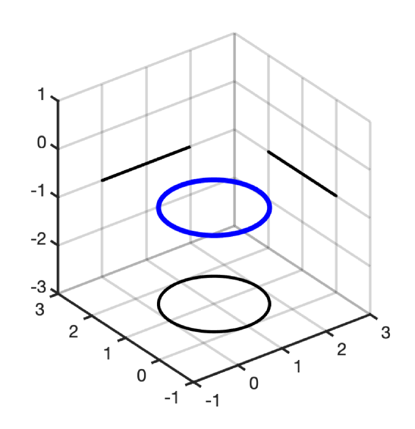
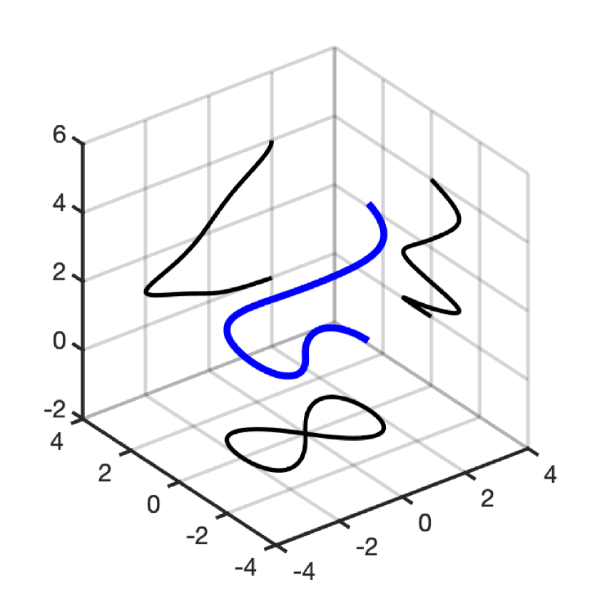
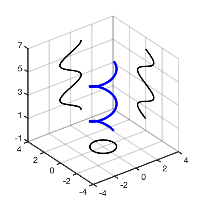
Figure 6.1: Center curves $K$ (solid blue) of $D_{\rho}$ in Examples 6.1 (left), 6.2 (center), and 6.3 (right). Plots also show projections of $K$ onto coordinate planes (solid black).

Example 6.1.

In the first example $D_{\rho}$ is a thin torus, where the center curve $K$ is a circle parametrized by ${\bm{p}}=(p_{1},p_{2},p_{3})^{\top}\in\mathcal{P}$ with

$$p_{1}(s)\,=\,\cos(2\pi s)+1\,,\quad p_{2}(s)\,=\,\sin(2\pi s)+1\,,\quad p_{3}(s)\,=\,-1\,,\qquad s\in[0,1]\,,$$

as shown in Figure 6.1 (left). The cross-section $D_{\rho}^{\prime}$ is a disk of radius $\rho>0$, and the material parameters of the scattering object are described by the relative electric permittivity $\varepsilon_{r}=2.5$ and the relative magnetic permeability $\mu_{r}=1.6$.  $\lozenge$

Example 6.2.

In the second example the scattering object $D_{\rho}$ is a thin tube with a center curve parametrized by ${\bm{p}}=(p_{1},p_{2},p_{3})^{\top}\in\mathcal{P}$ with

$$p_{1}(s)\,=\,2\frac{\cos(2\pi s)}{1+\sin(2\pi s)^{2}}\,,\quad p_{2}(s)\,=\,4\frac{\cos(2\pi s)\sin(2\pi s)}{1+2\sin(2\pi s)^{2}}\,,\quad p_{3}(s)\,=\,4s^{2}\,,\qquad s\in[0,1]\,,$$

as shown in Figure 6.1 (center). The cross-section $D_{\rho}^{\prime}$ is a disk of radius $\rho>0$, and the material parameters of the scattering object in this example are described by relative electric permittivity $\varepsilon_{r}=1.0$ and the relative magnetic permeability $\mu_{r}=2.1$, i.e., there is no permittivity contrast.  $\lozenge$

Example 6.3.

In the third example the scattering object $D_{\rho}$ is a thin tube with a center curve that is a two-turn helix parametrized by ${\bm{p}}=(p_{1},p_{2},p_{3})^{\top}\in\mathcal{P}$ with

$$p_{1}(s)\,=\,\cos(4\pi s)\,,\quad p_{2}(s)\,=\,\sin(4\pi s)\,,\quad p_{3}(s)\,=\,6s\,,\qquad s\in[0,1]\,,$$

a shown in Figure 6.1 (right). The cross-section $D_{\rho}^{\prime}$ is a disk of radius $\rho>0$, and the material parameters of the scattering object in this example are described by relative electric permittivity $\varepsilon_{r}=2.1$ and the relative magnetic permeability $\mu_{r}=1.0$, i.e., there is no permeability contrast.  $\lozenge$

6.1 The accuracy of the asymptotic representation formula

We discuss the accuracy of the approximation of the electric far field pattern ${\bm{E}}^{\infty}_{\rho}$ by the leading order term $\widetilde{{\bm{E}}^{\infty}_{\rho}}$ in the asymptotic perturbation formula (3.7). To quantify the approximation error we consider the relative difference

$$\mathtt{RelDiff}\,:=\,\frac{\|\widetilde{{\bm{E}}^{\infty}_{\rho}}-{\bm{E}}^{\infty}_{\rho}\|_{L^{2}({S^{2}})}}{\|{\bm{E}}^{\infty}_{\rho}\|_{L^{2}({S^{2}})}}\,.$$ (6.1)

Since the exact far field pattern ${\bm{E}}^{\infty}_{\rho}$ is unknown, we simulate accurate reference far field data ${\bm{E}}^{\infty}_{\rho}$ using the C++ boundary element library Bempp (see [42]). For this purpose, we consider an integral equation formulation of the electromagnetic scattering problem (2.10) that is based on the multitrace operator. The corresponding implementation in Bempp is described in detail in [41].

To evaluate $\mathtt{RelDiff}$ numerically, we approximate the vector fields $\widetilde{{\bm{E}}^{\infty}_{\rho}}$ and ${\bm{E}}^{\infty}_{\rho}$ on the equiangular grid on ${S^{2}}$ from (5.8) with $N=10$, and accordingly we discretize the $L^{2}$-norms in (6.1) using a composite trapezoid rule in horizontal and vertical direction. We discuss the following two questions:

1. How many spline segments and how many quadrature points per spline segment are sufficient in the approximation ${\bm{p}}_{\bigtriangleup}$ of the center curve $K$ that is used to evaluate $\widetilde{{\bm{E}}^{\infty}_{\rho}}$ numerically, to obtain a reasonably good approximation of ${\bm{E}}^{\infty}_{\rho}$?

2. How small does the radius $\rho>0$ of the thin tubular scattering object $D_{\rho}$ have to be in order that the leading order term $\widetilde{{\bm{E}}^{\infty}_{\rho}}$ in the asymptotic perturbation formula (3.7) is a sufficiently good approximation of ${\bm{E}}^{\infty}_{\rho}$?

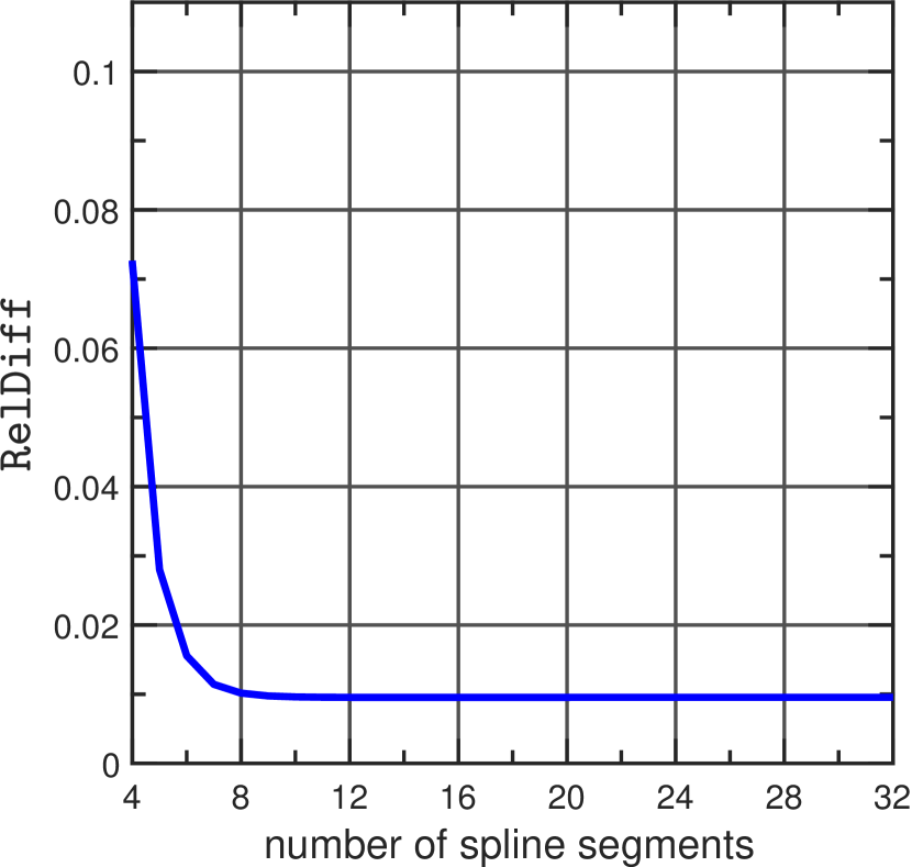
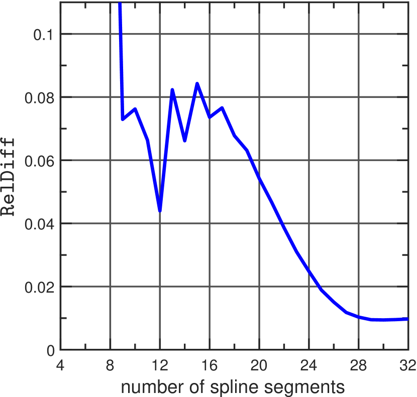
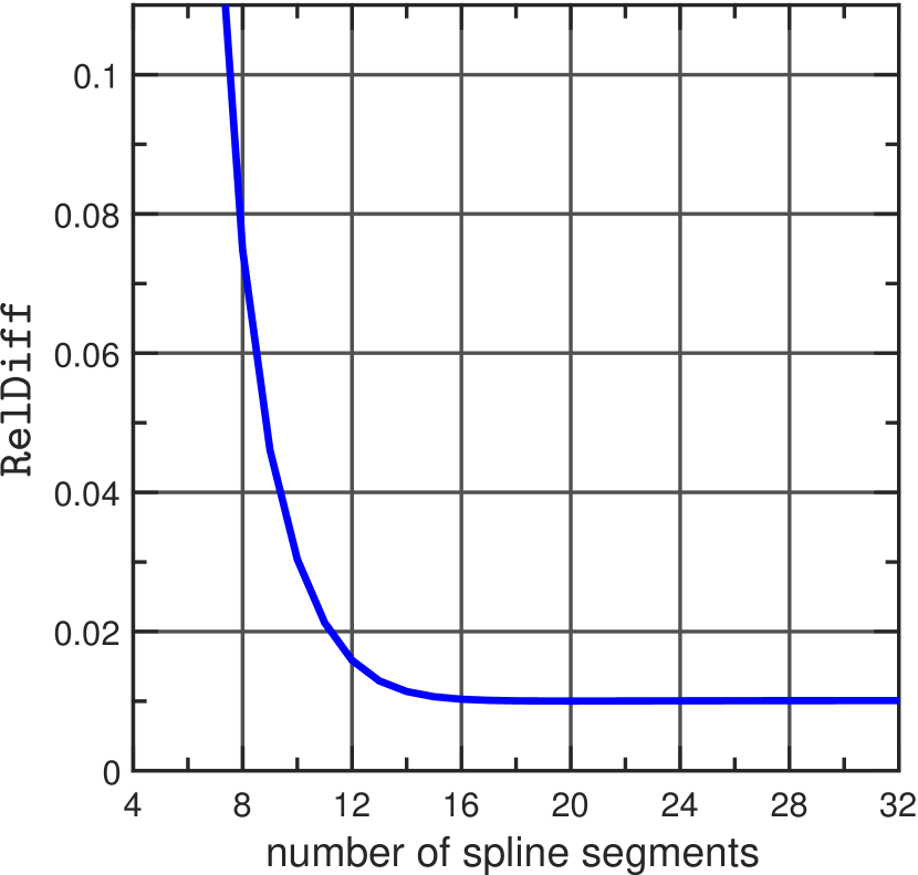
Figure 6.2: Relative difference $\mathtt{RelDiff}$ between ${\bm{E}}^{\infty}_{\rho}$ and the leading order term $\widetilde{{\bm{E}}^{\infty}_{\rho}}$ in (6.1) as a function of the number of subsegments in the spline approximation ${\bm{p}}_{\bigtriangleup}$ of the center curve $K$ for Examples 6.1 (left), 6.2 (center), and 6.3 (right) with radius $\rho=0.03$.

Concerning the first question, we consider the scattering objects in Examples 6.1, 6.2, and 6.3 with radius $\rho=0.03$, and we evaluate reference far field data ${\bm{E}}^{\infty}_{\rho}$ using Bempp as described above. In the corresponding Galerkin boundary element discretization we use a triangulation of the boundary of the scatterer $\partial D_{\rho}$ with 26698 triangles for Example 6.1, 62116 triangles for Example 6.2, and 62116 triangles for Example 6.3. Then we consider a sequence of increasingly fine equidistant partitions $\bigtriangleup$ of $[0,1]$ as in (5.6), we evaluate $\widetilde{{\bm{E}}^{\infty}_{\rho}}$ from (5.3), and we study the decay of the relative difference $\mathtt{RelDiff}$ from (6.1) as a function of the number of subsegments of the spline approximations ${\bm{p}}_{\bigtriangleup}$ of the center curves $K$. We approximate the integrals in (5.3) using a composite Simpson’s rule with a fixed number of $M=11$ nodes on each subinterval of $\bigtriangleup$. The results of these tests are shown in Figure 6.2. In each example the relative error decreases quickly until it reaches its minimum value. Due to the asymptotic character of the expansion (3.7), and due to numerical error in the numerical approximation of ${\bm{E}}^{\infty}_{\rho}$ obtained by Bempp, we do not expect the relative error $\mathtt{RelDiff}$ to decay to zero. A relatively low number of spline segments suffices in all three examples to obtain less than $2\%$ relative difference. Of course this number depends on the shape of the center curve. We note that while the simulation of ${\bm{E}}^{\infty}_{\rho}$ using Bempp is computationally quite demanding, the evaluation of $\widetilde{{\bm{E}}^{\infty}_{\rho}}$ using (5.3) is simple and extremely fast.

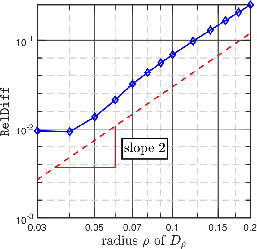
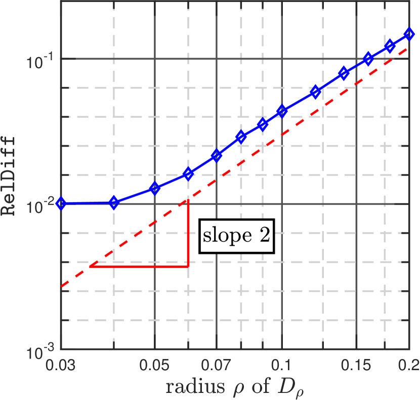
Figure 6.3: Relative difference $\mathtt{RelDiff}$ (solid blue) between ${\bm{E}}^{\infty}_{\rho}$ and the leading order term $\widetilde{{\bm{E}}^{\infty}_{\rho}}$ in (6.1) as a function of the radius $\rho$ of the thin tubular scatterer $D_{\rho}$ for Examples 6.1 (left), 6.2 (center), and 6.3 (right). For comparison the plot contains a line of slope $2$ (dashed red).

Concerning the second question from above we again generate reference far field data ${\bm{E}}^{\infty}_{\rho}$ for the thin tubular scattering objects in Examples 6.1–6.3 using Bempp, but now for a whole range of radii

$$\rho\in\{0.03,\,0.04,\,0.05,\,0.06,\,0.07,\,0.08,\,0.09,\,0.1,\,0.12,\,0.14,\,0.16,\,0.18,\,0.2\}\,.$$

Here we use increasingly fine triangulations of the boundaries of the scatterers $\partial D_{\rho}$. We also evaluate the approximations $\widetilde{{\bm{E}}^{\infty}_{\rho}}$ for these values of $\rho$ using $29$ spline segments in the spline approximations ${\bm{p}}_{\bigtriangleup}$ of the center curves $K$. In Figure 6.3 we show plots of the relative difference $\mathtt{RelDiff}$ as a function of $\rho$ (solid blue) for these three examples. For comparison these plots contain a line of slope $2$ (dashed red). The relative error decays approximately of order $\mathcal{O}(\rho^{2})$. We note that our theoretical results in Theorem 3.1 do not predict any rate of convergence.

6.2 Reconstruction of the center curve $K$ using Algorithm 5.1

We return to the inverse problem and apply Algorithm 5.1 to reconstruct the center curves $K$ of the thin tubular scattering objects $D_{\rho}$ in Examples 6.1–6.3 from observations of a single electric far field pattern ${\bm{E}}^{\infty}_{\rho}$. In all three examples the radius of the scattering object $D_{\rho}$ is $\rho=0.03$. The previous examples show that ${\bm{E}}^{\infty}_{\rho}$ is well approximated by $\widetilde{{\bm{E}}^{\infty}_{\rho}}$ in this regime. We assume that the plane wave incident field ${\bm{E}}^{i}$ (i.e., the wave number $k$, the direction of propagation ${\bm{\theta}}$, and the polarization ${\bm{A}}$), the shape and the radius of the cross-sections $D_{\rho}^{\prime}$ of the scattering objects (i.e., in particular $\rho$) and the material parameters of the scattering objects (i.e., the relative electric permittivity $\varepsilon_{r}$ and the relative magnetic permeability $\mu_{r}$) are known a priori.

We simulate the far field data ${\bm{E}}^{\infty}_{\rho}$ for each of the three examples using Bempp, where we use triangulations of the boundaries of the tubes $\partial D_{\rho}$ with 26698 triangles for Example 6.1, 62116 triangles for Example 6.2, and 62116 triangles for Example 6.3. The values of ${\bm{E}}^{\infty}_{\rho}$ are evaluated on the equiangular grid on ${S^{2}}$ from (5.8) with $N=10$.

We choose the following parameters in Algorithm 5.1:

• We use $n=30$ control points (i.e. $29$ spline segments) in the spline approximation ${\bm{p}}_{\bigtriangleup}$ of the unknown center curve $K$.

• We initialize the regularization parameters in step 2 by $\alpha_{1}=0.2$ and $\alpha_{2}=0.9$.

• We choose $s_{\mathrm{max}}=1$ in the golden section line search in step 5 and we terminate each line search after a fixed number of $10$ steps.

The results are shown in Figures 6.4–6.6. Here, the top-left plots show the initial guess, and the bottom-right plots show the final reconstruction. The remaining four plots show intermediate approximations of the iterative reconstruction procedure. Each plot contains the exact center curve $K$ (solid blue) and the current approximation ${\bm{p}}_{\bigtriangleup,\ell}$ of the reconstruction algorithm after $\ell$ iterations (solid red with stars). Furthermore, we have included projections of these curves onto the three coordinate planes to enhance the three-dimensional perspective.

Example 6.4.

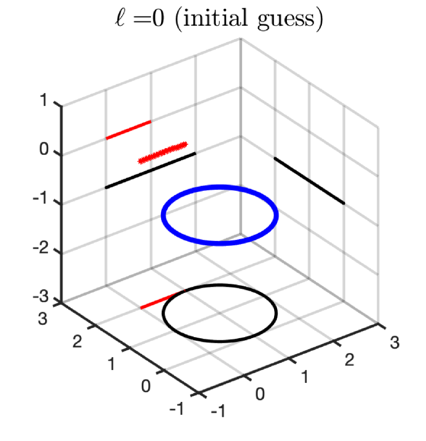
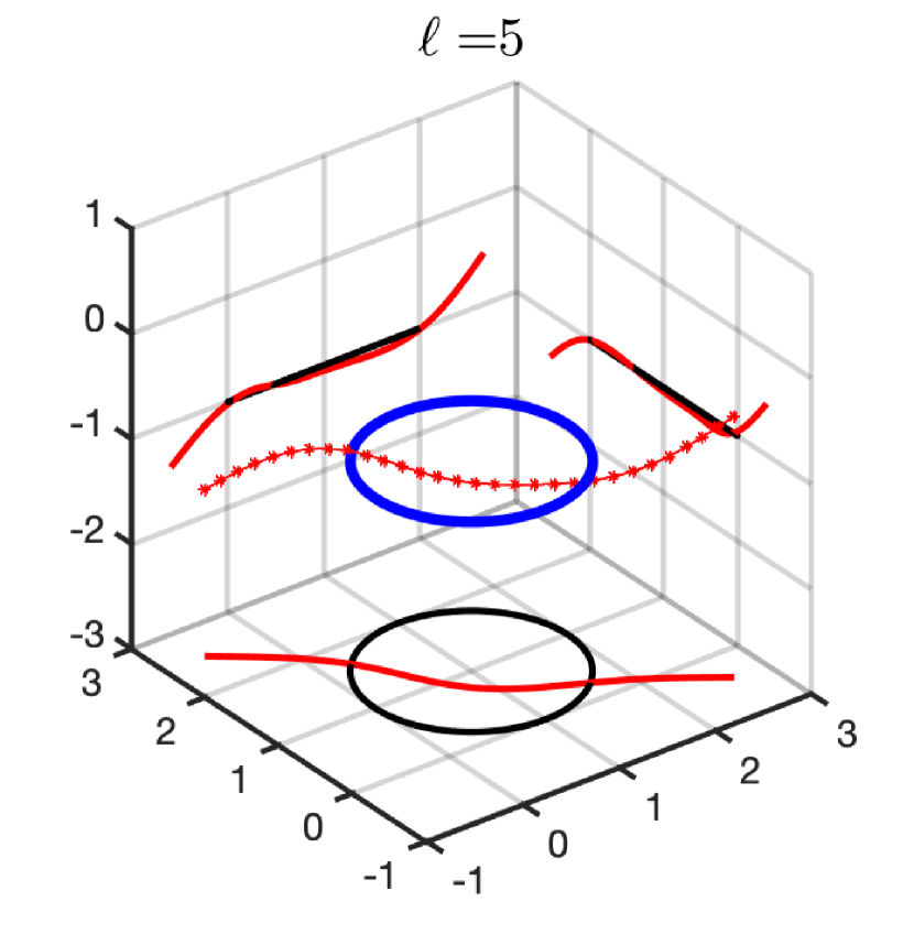
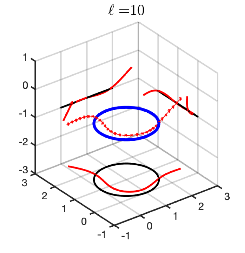
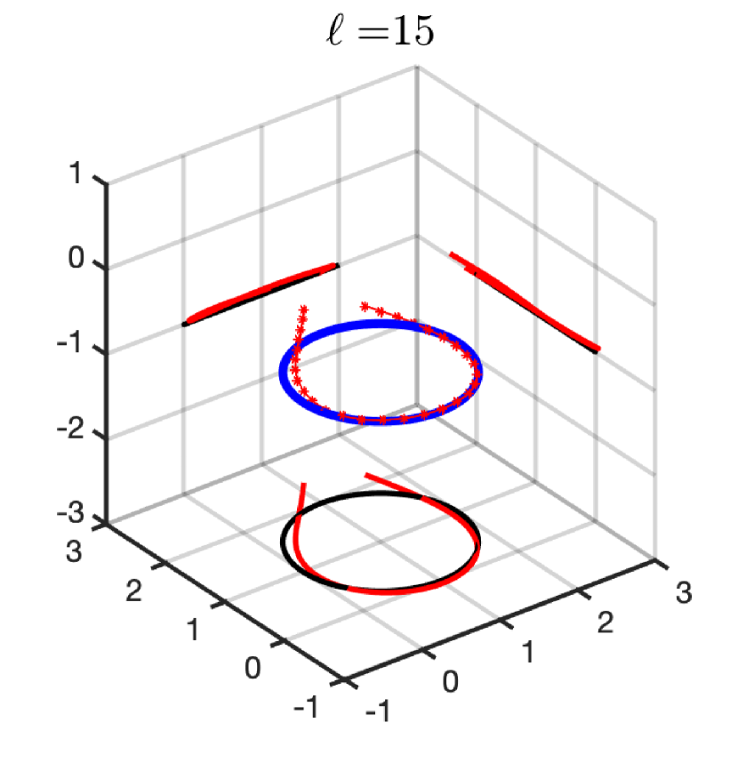
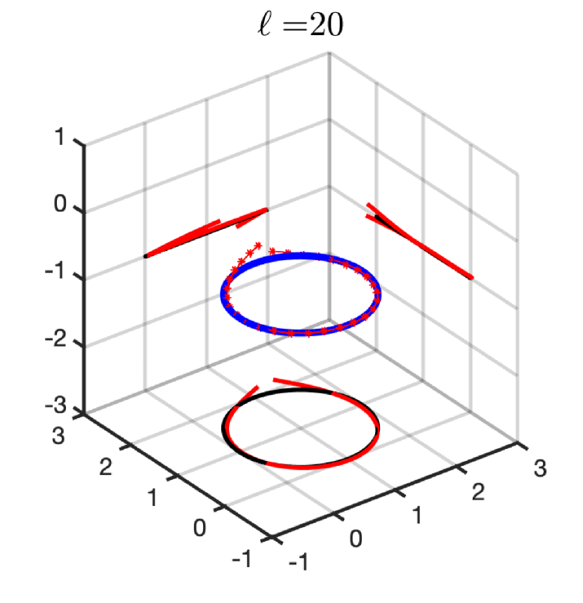
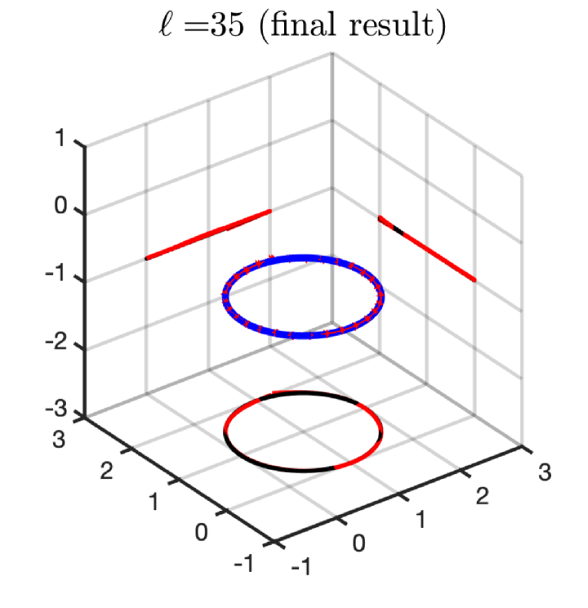
Figure 6.4: Reconstruction of the toroidal scatterer from Example 6.1. The top-left plot shows the initial guess, and the bottom-right plot shows the final reconstruction.

We consider the setting from Example 6.1. The initial guess is a straight line segment connecting the points $[0,2,0]^{\top}$ and $[1,2,0]^{\top}$. The reconstruction algorithm stops after $35$ iterations. The initial guess, some intermediate steps and the final result of the reconstruction algorithm are shown in Figure 6.4. The final reconstruction is very close to the exact center curve $K$.  $\lozenge$

Example 6.5.

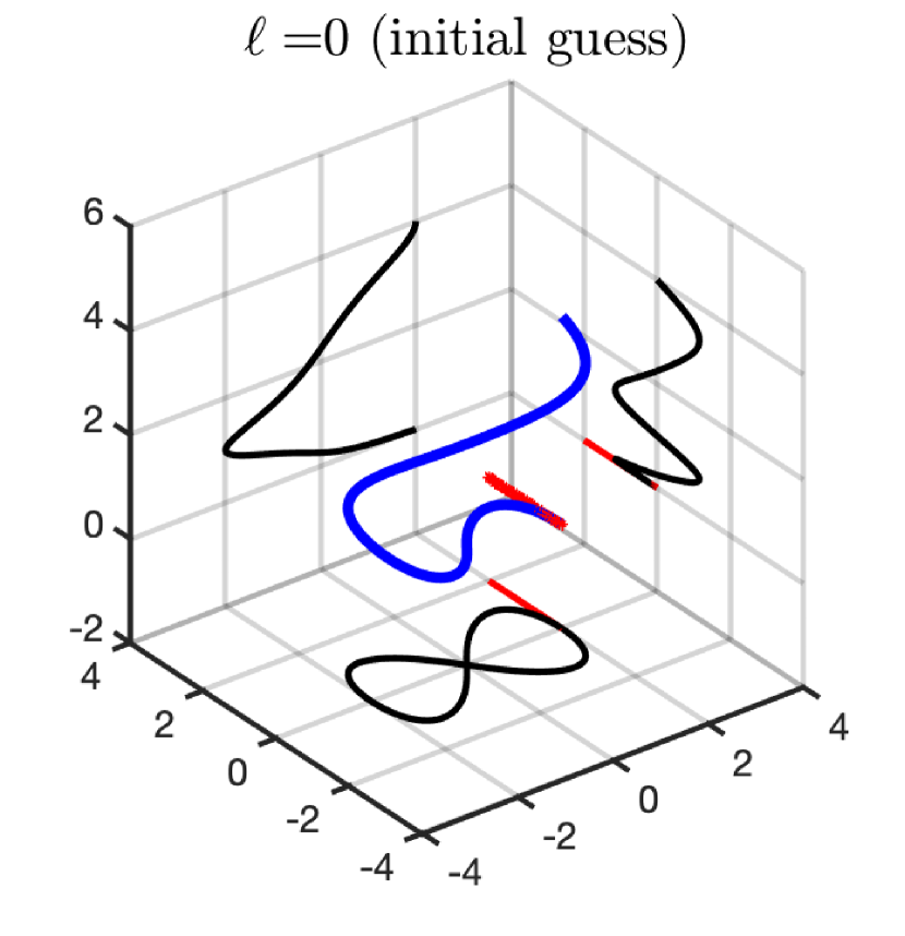
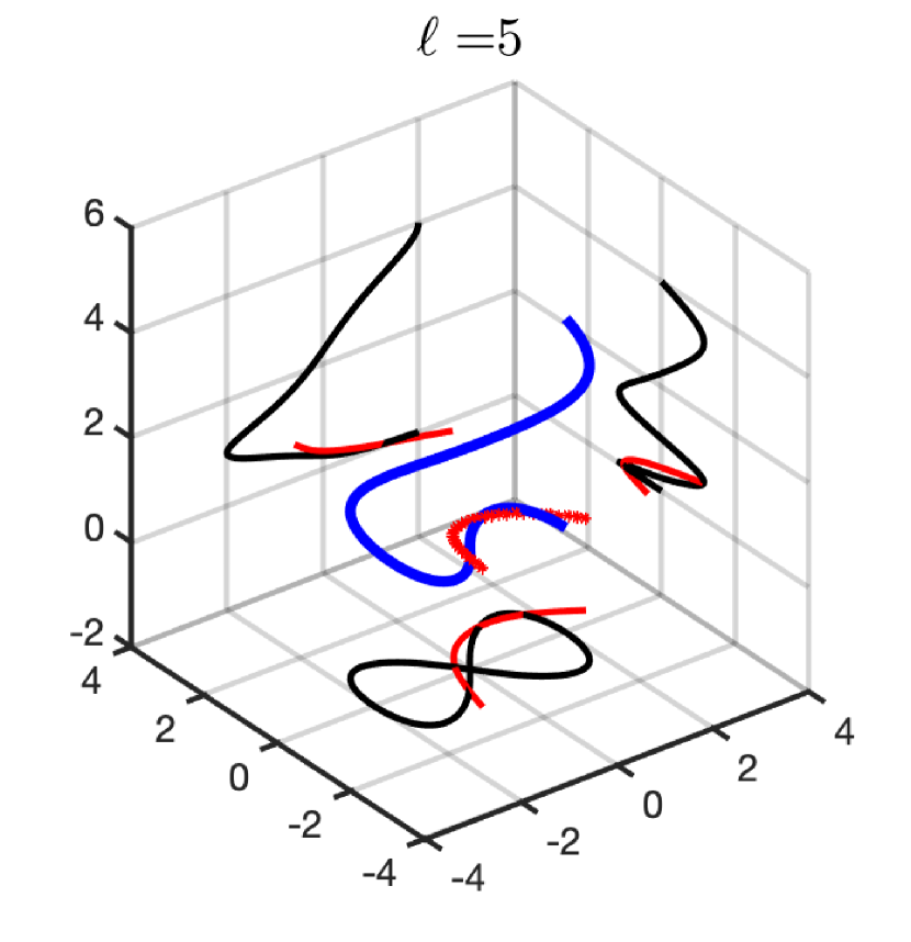
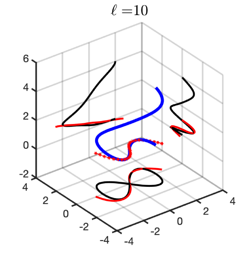
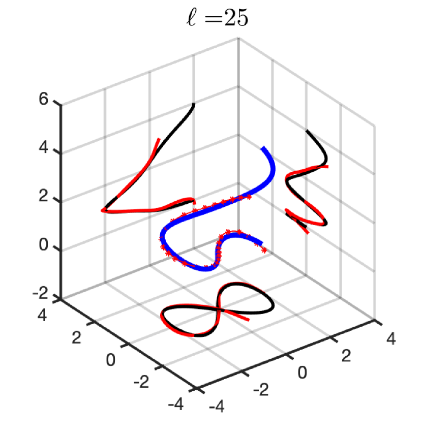
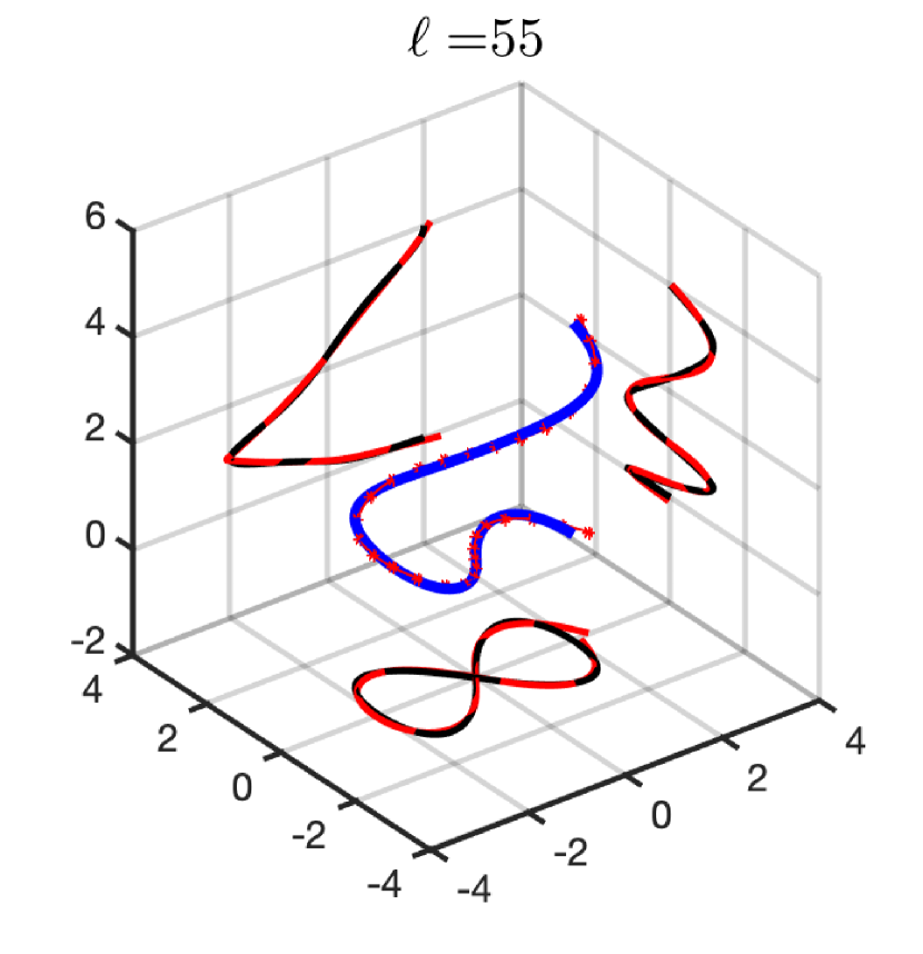
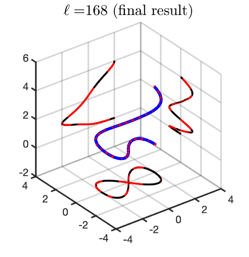
Figure 6.5: Reconstruction of the thin tubular scatterer from Example 6.2. The top-left plot shows the initial guess, and the bottom-right plot shows the final reconstruction.

We consider the setting from Example 6.2. The initial guess is a straight line segment connecting the points $[2,0,0]^{\top}$ and $[2,2,0]^{\top}$. The reconstruction algorithm stops after $168$ steps. The initial guess, some intermediate steps and the final result of the reconstruction algorithm are shown in Figure 6.5. Again the final reconstruction is very close to the exact center curve $K$. $\lozenge$

Example 6.6.

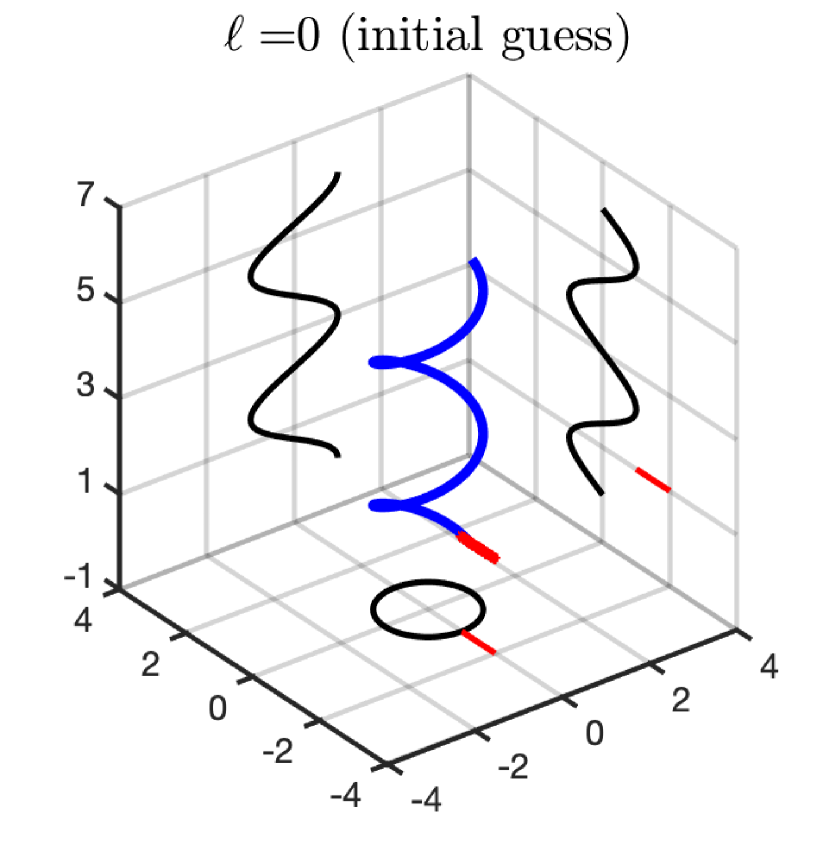
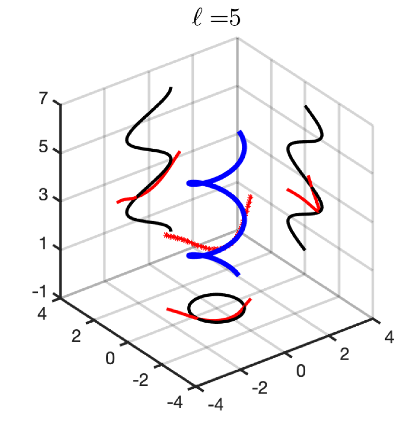
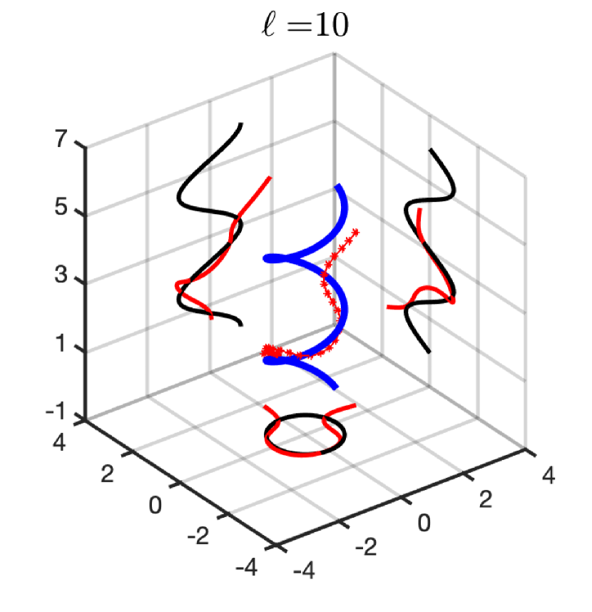
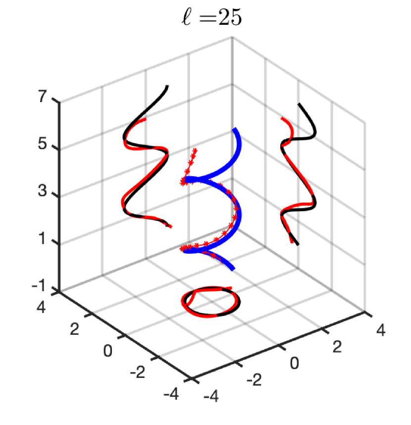
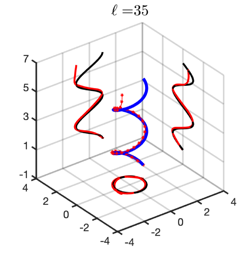
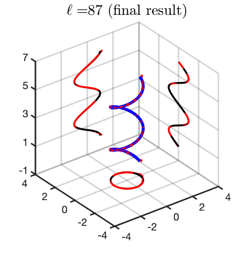
Figure 6.6: Reconstruction of the helical scatterer from Example 6.3. The top-left plot shows the initial guess, and the bottom-right plot shows the final reconstruction.

We consider the setting from Example 6.3. The initial guess is a straight line segment connecting the points $[0,-1,1]^{\top}$ and $[0,-2,1]^{\top}$. The reconstruction algorithm stops after $87$ steps. The initial guess, some intermediate steps and the final result of the reconstruction algorithm are shown in Figure 6.6. As in the previous examples, the final reconstruction is very close to the exact center curve $K$. $\lozenge$

In all three examples Algorithm 5.1 provides accurate approximations to the center curve $K$ of the unknown scattering object $D_{\rho}$. However, a suitable choice of the regularization parameters $\alpha_{1}$ and $\alpha_{2}$, and an initial guess ${\bm{p}}_{\bigtriangleup}$ sufficiently close to the unknown center curve $K$ are crucial for a successful reconstruction.

In our final example we study the sensitivity of the reconstruction algorithm to noise in the far field data.

Example 6.7.

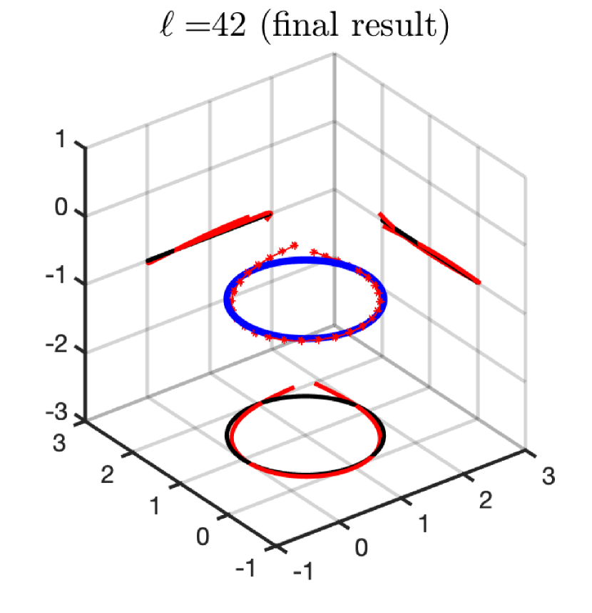
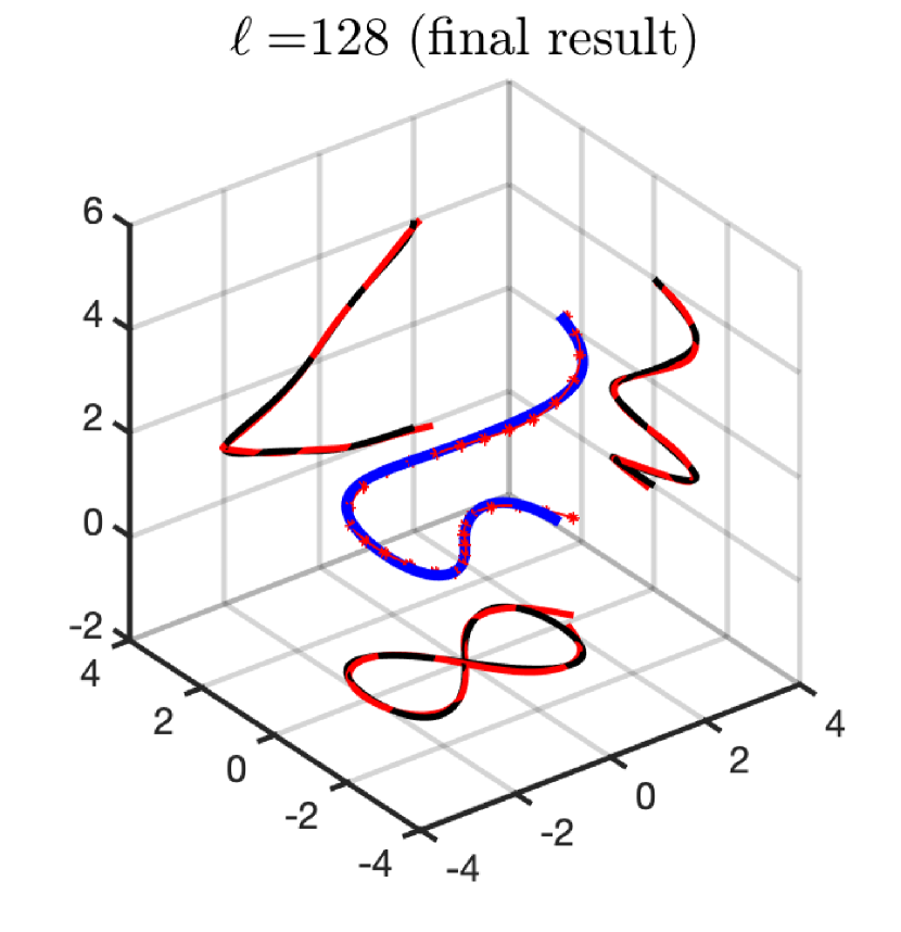
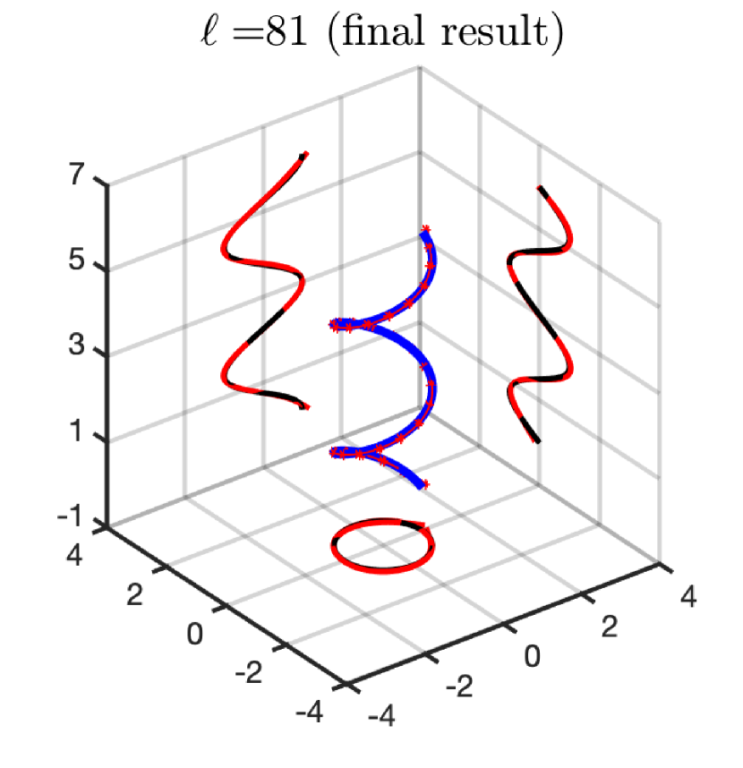
Figure 6.7: Reconstructions from noisy data with $30\%$ uniformly distributed additive noise.

We repeat the previous computations but we add $30\%$ complex-valued uniformly distributed error to the electric far field patterns ${\bm{E}}^{\infty}_{\rho}$ that have been simulates using Bempp. We use the same initial guesses and the same initial values for the regularization parameters $\alpha_{1}$ and $\alpha_{2}$ as in Examples 6.4–6.6. The three plots in Figure 6.7 show the exact center curves (solid blue), the final reconstructions (solid red with stars), and the projections of these curves onto the coordinate planes. The reconstruction algorithm stops after $42$ iterations for Example 6.4, after $128$ iterations for Example 6.5, and after $81$ iterations for Example 6.6, respectively. Despite the relatively high noise level, the final reconstructions are still very close to the exact center curves $K$.

We note that Algorithm  5.1 incorporates all available a priori information about the radius $\rho$ and the shape of the cross-section of the unknown scatterer, and its material parameters $\varepsilon_{r}$ and $\mu_{r}$. Furthermore it reconstructs a relatively low number of control points corresponding to the spline approximation ${\bm{p}}_{\bigtriangleup}$ of the center curve $K$ of the unknown thin tubular scattering object $D_{\rho}$. We also have carefully regularized the output least squares functional $\Phi$ in (5.7). This might explain the good performance of the reconstruction algorithm even for rather noisy far field data. $\lozenge$

Conclusions

The scattered electromagnetic field due to a thin tubular scattering object in homogeneous free space can be approximated efficiently using an asymptotic representation formula in terms of the dyadic Green’s function of the background medium, the incident electromagnetic field, and two polarization tensors that encode the shape and the material parameters of the thin tubular scatterering object. In this work we have shown that, for a thin tubular scattering object with a fixed cross-section that possibly twists along the center curve, these three-dimensional polarization tensors can be computed from the parametrization of the center curve and the two-dimensional polarization tensors of the cross-section.

For sufficiently regular cross-sections these two-dimensional polarization tensors can be approximated by solving a two-dimensional transmission problem for the Laplace equation. For ellipsoidal cross-sections explicit formulas are available. This gives a very efficient tool to analyze and simulate scattered fields due to thin tubular structures.

We have applied these results to develop an efficient iterative reconstruction method to recover the center curve of a thin tubular scattering object from far field observations of a single scattered field. Our numerical examples illustrate the accuracy of the asymptotic perturbation formula and the performance of the iterative reconstruction method.

Appendix

Appendix A Local coordinates

In this section we derive the Jacobian determinant $J_{\Gamma}$ and compute the gradient in the local coordinate system ${\bm{r}}_{\Gamma}$ from (2.4). The Frenet-Serret formulas state that the Frenet-Serret frame $({\bm{t}}_{\Gamma},{\bm{n}}_{\Gamma},{\bm{b}}_{\Gamma})$ from (2.2) satisfies

$$\frac{\partial{\bm{t}}_{\Gamma}}{\partial s}\,=\,\kappa{\bm{n}}_{\Gamma}\,,\qquad\frac{\partial{\bm{b}}_{\Gamma}}{\partial s}\,=\,-\tau{\bm{n}}_{\Gamma}\,,\qquad\frac{\partial{\bm{n}}_{\Gamma}}{\partial s}\,=\,\tau{\bm{b}}_{\Gamma}-\kappa{\bm{t}}_{\Gamma}\,.$$

Therewith we find that

$$\begin{split}\frac{\partial{\bm{r}}_{\Gamma}}{\partial s}(s,\eta,\zeta)&\,=\,{\bm{t}}_{\Gamma}(s)\Bigl{(}1-\kappa(s)\begin{bmatrix}1&0\end{bmatrix}R_{\theta}(s)\begin{bmatrix}\eta\\ \zeta\end{bmatrix}\Bigr{)}\\ &\phantom{\,=\,}+\begin{bmatrix}{\bm{n}}_{\Gamma}(s)&{\bm{b}}_{\Gamma}(s)\end{bmatrix}\biggl{(}\begin{bmatrix}0&-\tau(s)\\ \tau(s)&0\end{bmatrix}R_{\theta}(s)+\frac{\partial R_{\theta}}{\partial s}(s)\biggr{)}\begin{bmatrix}\eta\\ \zeta\end{bmatrix}\,,\\ \frac{\partial{\bm{r}}_{\Gamma}}{\partial\eta}(s,\eta,\zeta)&\,=\,\begin{bmatrix}{\bm{n}}_{\Gamma}(s)&{\bm{b}}_{\Gamma}(s)\end{bmatrix}R_{\theta}(s)\begin{bmatrix}1\\ 0\end{bmatrix}\,,\\ \frac{\partial{\bm{r}}_{\Gamma}}{\partial\zeta}(s,\eta,\zeta)&\,=\,\begin{bmatrix}{\bm{n}}_{\Gamma}(s)&{\bm{b}}_{\Gamma}(s)\end{bmatrix}R_{\theta}(s)\begin{bmatrix}0\\ 1\end{bmatrix}\,.\end{split}$$

Accordingly,

$$J_{\Gamma}(s,\eta,\zeta)\,:=\,\det D{\bm{r}}_{\Gamma}(s,\eta,\zeta)\,=\,1-\kappa(s)\begin{bmatrix}1&0\end{bmatrix}R_{\theta}(s)\begin{bmatrix}\eta\\ \zeta\end{bmatrix}\,.$$

Furthermore, applying the chain rule we obtain that

$$\begin{split}\frac{\partial u\circ{\bm{r}}_{\Gamma}}{\partial s}(s,\eta,\zeta)&\,=\,\nabla u(s,\eta,\zeta)\cdot\biggl{(}{\bm{t}}_{\Gamma}(s)\Bigl{(}1-\kappa(s)\begin{bmatrix}1&0\end{bmatrix}R_{\theta}(s)\begin{bmatrix}\eta\\ \zeta\end{bmatrix}\Bigr{)}\\ &\phantom{\,=\,\nabla u(s,\eta,\zeta)\cdot\Bigl{(}}+\begin{bmatrix}{\bm{n}}_{\Gamma}(s)&{\bm{b}}_{\Gamma}(s)\end{bmatrix}\Bigl{(}\begin{bmatrix}0&-\tau(s)\\ \tau(s)&0\end{bmatrix}R_{\theta}(s)+\frac{\partial R_{\theta}}{\partial s}(s)\Bigr{)}\begin{bmatrix}\eta\\ \zeta\end{bmatrix}\biggr{)}\,,\\ \frac{\partial u\circ{\bm{r}}_{\Gamma}}{\partial\eta}(s,\eta,\zeta)&\,=\,\nabla u(s,\eta,\zeta)\cdot\Bigl{(}\begin{bmatrix}{\bm{n}}_{\Gamma}(s)&{\bm{b}}_{\Gamma}(s)\end{bmatrix}R_{\theta}(s)\begin{bmatrix}1\\ 0\end{bmatrix}\Bigr{)}\,,\\ \frac{\partial u\circ{\bm{r}}_{\Gamma}}{\partial\zeta}(s,\eta,\zeta)&\,=\,\nabla u(s,\eta,\zeta)\cdot\Bigl{(}\begin{bmatrix}{\bm{n}}_{\Gamma}(s)&{\bm{b}}_{\Gamma}(s)\end{bmatrix}R_{\theta}(s)\begin{bmatrix}0\\ 1\end{bmatrix}\Bigr{)}\,.\end{split}$$

Using the orthogonal decomposition

$$\nabla u\,=\,({\bm{t}}_{\Gamma}\cdot\nabla u){\bm{t}}_{\Gamma}+({\bm{n}}_{\Gamma}\cdot\nabla u){\bm{n}}_{\Gamma}+({\bm{b}}_{\Gamma}\cdot\nabla u){\bm{b}}_{\Gamma}$$

and the notation

$$\nabla_{\eta,\zeta}^{\prime}u\circ{\bm{r}}_{\Gamma}\,:=\,\begin{bmatrix}\frac{\partial u\circ{\bm{r}}_{\Gamma}}{\partial\eta}&\frac{\partial u\circ{\bm{r}}_{\Gamma}}{\partial\zeta}\end{bmatrix}^{\top}$$

for the two-dimensional gradient with respect to $(\eta,\zeta)$, we find that the gradient satisfies

$$\nabla u({\bm{r}}_{\Gamma}(s,\eta,\zeta))\,=\,J_{\Gamma}^{-1}(s,\eta,\zeta)\biggl{(}\frac{\partial u\circ{\bm{r}}_{\Gamma}}{\partial s}(s,\eta,\zeta)+\Bigl{(}\tau+\frac{\partial\theta}{\partial s}\Bigr{)}(s)\begin{bmatrix}\zeta\\ -\eta\end{bmatrix}\cdot\bigl{(}\nabla_{\eta,\zeta}^{\prime}u\circ{\bm{r}}_{\Gamma}\bigr{)}(s,\eta,\zeta)\biggr{)}{\bm{t}}_{\Gamma}(s)\\ +\begin{bmatrix}{\bm{n}}_{\Gamma}(s)&{\bm{b}}_{\Gamma}(s)\end{bmatrix}R_{\theta}(s)\bigl{(}\nabla_{\eta,\zeta}^{\prime}u\circ{\bm{r}}_{\Gamma}\bigr{)}(s,\eta,\zeta)\,.$$

Appendix B Some estimates

In the following we collect some estimates that are used in the proof of Proposition 4.2 (see also [18] for (B.2a)–(B.2b)).

Lemma B.1.

Suppose $D\subseteq\Omega\subseteq{\mathbb{R}}^{d}$, $d=2,3$, let $\gamma_{0},\gamma_{1}>0$, and let $\gamma\in L^{\infty}(\Omega)$ be defined by

$$\gamma\,:=\,\begin{cases}\gamma_{1}\,,&{\bm{x}}\in D\,,\\ \gamma_{0}\,,&{\bm{x}}\in{\mathbb{R}}^{d}\setminus\overline{D}\,,\end{cases}$$

Given ${\bm{F}}\in L^{\infty}(\Omega,{\mathbb{R}}^{d})$, we denote by $w\in H^{1}_{0}(\Omega)$ the unique solution to

$$\mathrm{div}(\gamma\nabla w)\,=\,\mathrm{div}(\chi_{D}{\bm{F}})\quad\text{in $\Omega$}\,,\qquad w\,=\,0\quad\text{on $\partial\Omega$}\,.$$ (B.1)

Then, there exist constants $C,C_{p}>0$ such that

$$\|\nabla w\|_{L^{2}(\Omega)} \,\leq\,C|D|^{\frac{1}{2}}\|{\bm{F}}\|_{L^{\infty}(D)}\,,$$ (B.2a)

$$\|w\|_{L^{2}(\Omega)} \,\leq\,C|D|^{\frac{3}{4}}\|{\bm{F}}\|_{L^{\infty}(D)}\,,$$ (B.2b)

$$\|w\|_{W^{1,p}(\Omega)} \,\leq\,C_{p}|D|^{\frac{1}{p}}\|{\bm{F}}\|_{L^{\infty}(D)}\,,\qquad 1<p<2\,.$$ (B.2c)

Proof.

Using the weak formulation of (B.1) and Hölder’s inequality we find that

$$\|\nabla w\|_{L^{2}(\Omega)}^{2}\,\leq\,C\int_{\Omega}\gamma\nabla w\cdot\nabla w\,\operatorname{d\!}{\bm{x}}\,=\,C\int_{\Omega}\chi_{D}{\bm{F}}\cdot\nabla w\,\operatorname{d\!}{\bm{x}}\,\leq\,C|D|^{\frac{1}{2}}\|\nabla w\|_{L^{2}(\Omega)}\|{\bm{F}}\|_{L^{\infty}(D)}\,.$$

This gives (B.2a).

Let $z\in H^{1}_{0}(\Omega)$ be the unique solution to

$$\mathrm{div}(\gamma_{0}\nabla z)\,=\,-w\quad\text{in $\Omega$}\,,\qquad z\,=\,0\quad\text{on $\partial\Omega$}\,.$$ (B.3)

Elliptic regularity results (see, e.g., [26, Thm. 8.13]) show that $\|z\|_{H^{3}(\Omega)}\leq C\|w\|_{H^{1}(\Omega)}$, and Sobolev’s embedding theorem (see, e.g., [26, p. 158]) gives $\|\nabla z\|_{L^{\infty}(\Omega)}\leq C\|z\|_{H^{3}(\Omega)}$. Using the weak formulations of (B.3) and (B.1) we find that

$$\begin{split}\|w\|_{L^{2}(\Omega)}^{2}&\,=\,\int_{\Omega}\gamma_{0}\nabla z\cdot\nabla w\,\operatorname{d\!}{\bm{x}}\,=\,\int_{\Omega}\chi_{D}{\bm{F}}\cdot\nabla z\,\operatorname{d\!}{\bm{x}}+\int_{\Omega}(\gamma_{0}-\gamma)\nabla z\cdot\nabla w\,\operatorname{d\!}{\bm{x}}\\ &\,\leq\,\bigl{(}\|\chi_{D}{\bm{F}}\|_{L^{1}(\Omega)}+\|(\gamma_{0}-\gamma)\nabla w\|_{L^{1}(\Omega)}\bigr{)}\|\nabla z\|_{L^{\infty}(\Omega)}\\ &\,\leq\,C\bigl{(}|D|\|{\bm{F}}\|_{L^{\infty}(D)}+|D|^{\frac{1}{2}}\|\nabla w\|_{L^{2}(\Omega)}\bigr{)}\|w\|_{H^{1}(\Omega)}\,.\end{split}$$

Applying Poincare’s inequality and (B.2a) this shows (B.2b).

Next we note that

$$\mathrm{div}(\gamma_{0}\nabla w)\,=\,\mathrm{div}(\chi_{D}{\bm{F}})+\mathrm{div}\bigl{(}(\gamma_{0}-\gamma)\nabla w\bigr{)}\,.$$

If $1<p<2$, then the right hand side is in $W^{-1,p}(\Omega)$, and since $-\mathrm{div}(\gamma_{0}\nabla\cdot)$ is an isomorphism from $W^{1,p}_{0}(\Omega)$ to $W^{-1,p}(\Omega)$ (see, e.g., [11, p. 40]), we find using Hölder’s inequality and (B.2a) that

$$\begin{split}\|w\|_{W^{1,p}(\Omega)}&\,\leq\,C_{p}\|\chi_{D}{\bm{F}}\|_{L^{p}(\Omega)}+C_{p}\|(\gamma_{0}-\gamma)\nabla w\|_{L^{p}(\Omega)}\\ &\,\leq\,C_{p}|D|^{\frac{1}{p}}\|{\bm{F}}\|_{L^{\infty}(D)}+C_{p}|D|^{\frac{1}{p}-\frac{1}{2}}\|\nabla w\|_{L^{2}(\Omega)}\,\leq\,C_{p}|D|^{\frac{1}{p}}\|{\bm{F}}\|_{L^{\infty}(D)}\,.\end{split}$$

This gives (B.2c). ∎

The next lemma is used in the proof of Theorem 4.1 (b).

Lemma B.2.

Let $0<\rho<r/2$ and let $D_{\rho}^{\prime}\subseteq B_{\rho}^{\prime}(0)$ be open, where $B_{\rho}^{\prime}(0)\subseteq{\mathbb{R}}^{2}$ denotes the disk of radius $\rho$ around zero. Suppose that $A_{0},A_{1}\in C^{0,1}(B_{r}^{\prime}(0),{\mathbb{R}}^{2\times 2})$ are symmetric and

$$c^{-1}\,\leq\,{\bm{\xi}}^{\prime}\cdot A_{j}({\bm{x}}^{\prime}){\bm{\xi}}^{\prime}\,\leq\,c\qquad\text{for all }{\bm{x}}^{\prime}\in B_{r}^{\prime}(0)\,,\;{\bm{\xi}}^{\prime}\in{S^{2}}\,,\text{ and }j=1,2\,,$$

with some constant $c>0$, and let ${\bm{F}}\in C^{0,1}(B_{r}^{\prime}(0),{\mathbb{R}}^{2})$. We define $A_{\rho},{\widetilde{A}}_{\rho}\in C^{0,1}(B_{r}^{\prime}(0),{\mathbb{R}}^{2\times 2})$ by

$$A_{\rho}({\bm{x}}^{\prime})\,:=\,\begin{cases}A_{1}\,,&{\bm{x}}^{\prime}\in D_{\rho}\,,\\ A_{0}\,,&{\bm{x}}^{\prime}\in B_{r}^{\prime}(0)\setminus\overline{D_{\rho}}\,,\end{cases}\qquad\text{and}\qquad{\widetilde{A}}_{\rho}({\bm{x}}^{\prime})\,:=\,\begin{cases}A_{1}(0)\,,&{\bm{x}}^{\prime}\in D_{\rho}\,,\\ A_{0}(0)\,,&{\bm{x}}^{\prime}\in B_{r}^{\prime}(0)\setminus\overline{D_{\rho}}\,,\end{cases}$$

and we consider the unique solutions $w_{\rho},\widetilde{w}_{\rho}\in H^{1}_{0}(B_{r}^{\prime}(0))$ to

$$\mathrm{div}(A_{\rho}w_{\rho}) \,=\,\mathrm{div}(\chi_{D_{\rho}}{\bm{F}})\quad\text{in }B_{r}^{\prime}(0)\,,\qquad w_{\rho}=0\quad\text{on }\partial B_{r}^{\prime}(0)\,,$$ (B.4a)

$$\mathrm{div}({\widetilde{A}}_{\rho}\widetilde{w}_{\rho}) \,=\,\mathrm{div}(\chi_{D_{\rho}}{\bm{F}})\quad\text{in }B_{r}^{\prime}(0)\,,\qquad\widetilde{w}_{\rho}=0\quad\text{on }\partial B_{r}^{\prime}(0)\,.$$ (B.4b)

Then,

$$\bigl{\|}\nabla w_{\rho}-\nabla\widetilde{w}_{\rho}\bigr{\|}_{L^{2}(B_{r}^{\prime}(0))}\,=\,o(|D_{\rho}|^{\frac{1}{2}})\qquad\text{as }\rho\to 0\,.$$ (B.5)

Proof.

Using (B.4a) we find that

$$\mathrm{div}({\widetilde{A}}_{\rho}\nabla w_{\rho})\,=\,\mathrm{div}(\chi_{D_{\rho}}{\bm{F}}(0))+\mathrm{div}\bigl{(}\chi_{D_{\rho}}({\bm{F}}-{\bm{F}}(0))\bigr{)}+\mathrm{div}\bigl{(}({\widetilde{A}}_{\rho}-A_{\rho})\nabla w_{\rho}\bigr{)}\qquad\text{in }B_{r}^{\prime}(0)\,.$$

Therefore, introducting $\Omega^{\prime}:=B_{\rho^{1/4}}^{\prime}(0)$ we can write $w_{\rho}=\widetilde{w}_{\rho}+v_{1}+v_{2}+v_{3}$, where $v_{1},v_{2},v_{3}\in H^{1}_{0}(B_{r}^{\prime}(0))$ are the unique solutions to

$$\mathrm{div}({\widetilde{A}}_{\rho}v_{1}) \,=\,\mathrm{div}\bigl{(}\chi_{D_{\rho}}({\bm{F}}-{\bm{F}}(0))\bigr{)} \text{in }B_{r}^{\prime}(0)\,, v_{1}=0\quad\text{on }\partial B_{r}^{\prime}(0)\,,$$ (B.6a)

$$\mathrm{div}({\widetilde{A}}_{\rho}v_{2}) \,=\,\mathrm{div}\bigl{(}\chi_{\Omega^{\prime}}({\widetilde{A}}_{\rho}-A_{\rho})\nabla w_{\rho}\bigr{)} \text{in }B_{r}^{\prime}(0)\,, v_{2}=0\quad\text{on }\partial B_{r}^{\prime}(0)\,,$$ (B.6b)

$$\mathrm{div}({\widetilde{A}}_{\rho}v_{3}) \,=\,\mathrm{div}\bigl{(}(1-\chi_{\Omega^{\prime}})({\widetilde{A}}_{\rho}-A_{\rho})\nabla w_{\rho}\bigr{)} \text{in }B_{r}^{\prime}(0)\,, v_{3}=0\quad\text{on }\partial B_{r}^{\prime}(0)\,.$$ (B.6c)

Using (B.2a) and the Lipschitz continuity of ${\bm{F}}$ we find that

$$\|\nabla v_{1}\|_{L^{2}(B_{r}^{\prime}(0))}\,\leq\,C\|{\bm{F}}-{\bm{F}}(0)\|_{L^{\infty}(D_{\rho}^{\prime})}|D_{\rho}^{\prime}|^{\frac{1}{2}}\,\leq\,C\rho|D_{\rho}^{\prime}|^{\frac{1}{2}}\,=\,o(|D_{\rho}^{\prime}|^{\frac{1}{2}})\,.$$ (B.7)

Similarly, the well-posedness of (B.6b), (B.2a), and the Lipschitz continuity of $A_{0}$ and $A_{1}$ show that

$$\begin{split}\|\nabla v_{2}\|_{L^{2}(B_{r}^{\prime}(0))}&\,\leq\,C\bigl{\|}({\widetilde{A}}_{\rho}-A_{\rho})\chi_{\Omega^{\prime}}\bigl{\|}_{L^{\infty}(B_{r}^{\prime}(0))}\|\nabla w_{\rho}\|_{L^{2}(B_{r}^{\prime}(0))}\\ &\,\leq\,C\Bigl{(}\|A_{1}-A_{1}(0)\|_{L^{\infty}(D_{\rho}^{\prime})}+\|A_{0}-A_{0}(0)\|_{L^{\infty}(\Omega^{\prime})}\Bigr{)}|D_{\rho}^{\prime}|^{\frac{1}{2}}\\ &\,\leq\,C\bigl{(}\rho+\rho^{\frac{1}{4}}\bigr{)}|D_{\rho}^{\prime}|^{\frac{1}{2}}\,=\,o(|D_{\rho}^{\prime}|^{\frac{1}{2}})\,.\end{split}$$ (B.8)

Next let $h_{\rho}\in C^{1}([0,r])$ be a cut-off function satisfying

$$0\leq h_{\rho}\leq 1\,,\qquad\chi_{(0,\,\rho^{\frac{1}{2}})}h_{\rho}\,=\,0\,,\qquad\chi_{(\rho^{\frac{1}{4}},\,1)}h_{\rho}\,=\,\chi_{(\rho^{\frac{1}{4}},\,1)}\,,\qquad\|h_{\rho}^{\prime}\|_{L^{\infty}((0,\,r))}\,\leq\,C\rho^{-\frac{1}{4}}\,.$$ (B.9)

(see [13, Lmm. 3.6] for a similar construction). Using the weak formulation of (B.4a) and integrating by parts shows that

$$\begin{split}0&\,=\,\int_{D_{\rho}^{\prime}}{\bm{F}}\cdot\nabla(h_{\rho}^{2}w_{\rho})\,\operatorname{d\!}{\bm{x}}^{\prime}\,=\,\int_{B_{r}^{\prime}(0)}A_{\rho}\nabla w_{\rho}\cdot\nabla(h_{\rho}^{2}w_{\rho})\,\operatorname{d\!}{\bm{x}}^{\prime}\\ &\,=\,\int_{B_{r}^{\prime}(0)}A_{\rho}\nabla w_{\rho}\cdot\bigl{(}h_{\rho}\nabla(h_{\rho}w_{\rho})+h_{\rho}w_{\rho}\nabla h_{\rho}\bigr{)}\,\operatorname{d\!}{\bm{x}}^{\prime}\\ &\,=\,\int_{B_{r}^{\prime}(0)}A_{\rho}\nabla(h_{\rho}w_{\rho})\cdot\nabla(h_{\rho}w_{\rho})\,\operatorname{d\!}{\bm{x}}^{\prime}-\int_{B_{r}^{\prime}(0)}A_{\rho}w_{\rho}^{2}\nabla h_{\rho}\cdot\nabla h_{\rho}\,\operatorname{d\!}{\bm{x}}^{\prime}\,.\end{split}$$

Accordingly,

$$\|\nabla(h_{\rho}w_{\rho})\|_{L^{2}(B_{r}^{\prime}(0))}^{2}\,\leq\,C\|\nabla h_{\rho}\|_{L^{\infty}(B_{r}^{\prime}(0))}^{2}\|w_{\rho}\|_{L^{2}(B_{r}^{\prime}(0))}^{2}\,,$$

and applying (B.9) and (B.2b) gives

$$\|\nabla(h_{\rho}w_{\rho})\|_{L^{2}(B_{r}^{\prime}(0))}\,\leq\,C\rho^{-\frac{1}{4}}|D_{\rho}^{\prime}|^{\frac{3}{4}}\,\leq\,C|D_{\rho}^{\prime}|^{-\frac{1}{8}}|D_{\rho}^{\prime}|^{\frac{3}{4}}\,=\,o(|D_{\rho}^{\prime}|^{\frac{1}{2}})\,,$$

where we used that $D_{\rho}^{\prime}\subseteq B_{\rho}^{\prime}(0)$ and thus $|D_{\rho}^{\prime}|\leq\pi\rho^{2}$. Combining (B.6b) with (B.2a) we obtain that

$$\|v_{2}\|_{L^{2}(B_{r}^{\prime}(0))}\,\leq\,C\|\nabla w_{\rho}\|_{L^{2}(B_{r}^{\prime}(0)\setminus\overline{\Omega^{\prime}})}\,\leq\,C\|\nabla(h_{\rho}w_{\rho})\|_{L^{2}(B_{r}^{\prime}(0))}\,=\,o(|D_{\rho}^{\prime}|^{\frac{1}{2}})\,.$$ (B.10)

Finally, (B.7), (B.8), and (B.10) give (B.5). ∎

References

- [1] G. S. Alberti and Y. Capdeboscq. Lectures on elliptic methods for hybrid inverse problems, volume 25 of Cours Spécialisés [Specialized Courses]. Société Mathématique de France, Paris, 2018.
- [2] H. Ammari, E. Beretta, and E. Francini. Reconstruction of thin conductivity imperfections. Appl. Anal., 83(1):63–76, 2004.
- [3] H. Ammari, E. Beretta, and E. Francini. Reconstruction of thin conductivity imperfections. II. The case of multiple segments. Appl. Anal., 85(1-3):87–105, 2006.
- [4] H. Ammari, E. Iakovleva, and S. Moskow. Recovery of small inhomogeneities from the scattering amplitude at a fixed frequency. SIAM J. Math. Anal., 34(4):882–900, 2003.
- [5] H. Ammari and H. Kang. High-order terms in the asymptotic expansions of the steady-state voltage potentials in the presence of conductivity inhomogeneities of small diameter. SIAM J. Math. Anal., 34(5):1152–1166, 2003.
- [6] H. Ammari and H. Kang. Polarization and moment tensors, volume 162 of Applied Mathematical Sciences. Springer, New York, 2007. With applications to inverse problems and effective medium theory.
- [7] H. Ammari, H. Kang, G. Nakamura, and K. Tanuma. Complete asymptotic expansions of solutions of the system of elastostatics in the presence of an inclusion of small diameter and detection of an inclusion. J. Elasticity, 67(2):97–129 (2003), 2002.
- [8] H. Ammari, M. S. Vogelius, and D. Volkov. Asymptotic formulas for perturbations in the electromagnetic fields due to the presence of inhomogeneities of small diameter. II. The full Maxwell equations. J. Math. Pures Appl. (9), 80(8):769–814, 2001.
- [9] H. Ammari and D. Volkov. The leading-order term in the asymptotic expansion of the scattering amplitude of a collection of finite number of dielectric inhomogeneities of small diameter. International Journal for Multiscale Computational Engineering, 3(3), 2005.
- [10] J. M. Ball, Y. Capdeboscq, and B. Tsering-Xiao. On uniqueness for time harmonic anisotropic Maxwell’s equations with piecewise regular coefficients. Math. Models Methods Appl. Sci., 22(11):1250036, 11, 2012.
- [11] A. Bensoussan, J.-L. Lions, and G. Papanicolaou. Asymptotic analysis for periodic structures, volume 5 of Studies in Mathematics and its Applications. North-Holland Publishing Co., Amsterdam-New York, 1978.
- [12] E. Beretta, E. Bonnetier, E. Francini, and A. L. Mazzucato. Small volume asymptotics for anisotropic elastic inclusions. Inverse Probl. Imaging, 6(1):1–23, 2012.
- [13] E. Beretta, Y. Capdeboscq, F. de Gournay, and E. Francini. Thin cylindrical conductivity inclusions in a three-dimensional domain: a polarization tensor and unique determination from boundary data. Inverse Problems, 25(6):065004, 22, 2009.
- [14] E. Beretta and E. Francini. An asymptotic formula for the displacement field in the presence of thin elastic inhomogeneities. SIAM J. Math. Anal., 38(4):1249–1261, 2006.
- [15] E. Beretta, E. Francini, and M. S. Vogelius. Asymptotic formulas for steady state voltage potentials in the presence of thin inhomogeneities. A rigorous error analysis. J. Math. Pures Appl. (9), 82(10):1277–1301, 2003.
- [16] E. Beretta, M. Grasmair, M. Muszkieta, and O. Scherzer. A variational algorithm for the detection of line segments. Inverse Probl. Imaging, 8(2):389–408, 2014.
- [17] M. Brühl, M. Hanke, and M. S. Vogelius. A direct impedance tomography algorithm for locating small inhomogeneities. Numer. Math., 93(4):635–654, 2003.
- [18] Y. Capdeboscq and M. S. Vogelius. A general representation formula for boundary voltage perturbations caused by internal conductivity inhomogeneities of low volume fraction. M2AN Math. Model. Numer. Anal., 37(1):159–173, 2003.
- [19] Y. Capdeboscq and M. S. Vogelius. Optimal asymptotic estimates for the volume of internal inhomogeneities in terms of multiple boundary measurements. M2AN Math. Model. Numer. Anal., 37(2):227–240, 2003.
- [20] Y. Capdeboscq and M. S. Vogelius. A review of some recent work on impedance imaging for inhomogeneities of low volume fraction. In Partial differential equations and inverse problems, volume 362 of Contemp. Math., pages 69–87. Amer. Math. Soc., Providence, RI, 2004.
- [21] Y. Capdeboscq and M. S. Vogelius. Pointwise polarization tensor bounds, and applications to voltage perturbations caused by thin inhomogeneities. Asymptot. Anal., 50(3-4):175–204, 2006.
- [22] D. J. Cedio-Fengya, S. Moskow, and M. S. Vogelius. Identification of conductivity imperfections of small diameter by boundary measurements. Continuous dependence and computational reconstruction. Inverse Problems, 14(3):553–595, 1998.
- [23] C. Dapogny. The topological ligament in shape optimization: a connection with thin tubular inhomogeneities. Preprint, 2020.
- [24] C. Dapogny and M. S. Vogelius. Uniform asymptotic expansion of the voltage potential in the presence of thin inhomogeneities with arbitrary conductivity. Chin. Ann. Math. Ser. B, 38(1):293–344, 2017.
- [25] A. Friedman and M. Vogelius. Identification of small inhomogeneities of extreme conductivity by boundary measurements: a theorem on continuous dependence. Arch. Rational Mech. Anal., 105(4):299–326, 1989.
- [26] D. Gilbarg and N. S. Trudinger. Elliptic partial differential equations of second order. Classics in Mathematics. Springer-Verlag, Berlin, 2001. Reprint of the 1998 edition.
- [27] R. Griesmaier. Reconstruction of thin tubular inclusions in three-dimensional domains using electrical impedance tomography. SIAM J. Imaging Sci., 3(3):340–362, 2010.
- [28] R. Griesmaier. A general perturbation formula for electromagnetic fields in presence of low volume scatterers. ESAIM Math. Model. Numer. Anal., 45(6):1193–1218, 2011.
- [29] R. Griesmaier and N. Hyvönen. A regularized Newton method for locating thin tubular conductivity inhomogeneities. Inverse Problems, 27(11):115008, 22, 2011.
- [30] F. Hagemann, T. Arens, T. Betcke, and F. Hettlich. Solving inverse electromagnetic scattering problems via domain derivatives. Inverse Problems, 35(8):084005, 20, 2019.
- [31] F. Hettlich. The domain derivative of time-harmonic electromagnetic waves at interfaces. Math. Methods Appl. Sci., 35(14):1681–1689, 2012.
- [32] R. Lipton. Inequalities for electric and elastic polarization tensors with applications to random composites. J. Mech. Phys. Solids, 41(5):809–833, 1993.
- [33] R. A. Litherland, J. Simon, O. Durumeric, and E. Rawdon. Thickness of knots. Topology Appl., 91(3):233–244, 1999.
- [34] G. W. Milton. The theory of composites, volume 6 of Cambridge Monographs on Applied and Computational Mathematics. Cambridge University Press, Cambridge, 2002.
- [35] P. Monk. Finite element methods for Maxwell’s equations. Numerical Mathematics and Scientific Computation. Oxford University Press, New York, 2003.
- [36] A. B. Movchan and S. K. Serkov. The Pólya-Szegö matrices in asymptotic models of dilute composites. European J. Appl. Math., 8(6):595–621, 1997.
- [37] J. Nocedal and S. J. Wright. Numerical optimization. Springer Series in Operations Research. Springer-Verlag, New York, 1999.
- [38] W.-K. Park and D. Lesselier. Reconstruction of thin electromagnetic inclusions by a level-set method. Inverse Problems, 25(8):085010, 24, 2009.
- [39] G. Pólya and G. Szegö. Isoperimetric Inequalities in Mathematical Physics. Annals of Mathematics Studies, no. 27. Princeton University Press, Princeton, N. J., 1951.
- [40] M. Schiffer and G. Szegö. Virtual mass and polarization. Trans. Amer. Math. Soc., 67:130–205, 1949.
- [41] M. W. Scroggs, T. Betcke, E. Burman, W. Śmigaj, and E. van ’t Wout. Software frameworks for integral equations in electromagnetic scattering based on Calderón identities. Comput. Math. Appl., 74(11):2897–2914, 2017.
- [42] W. Śmigaj, T. Betcke, S. Arridge, J. Phillips, and M. Schweiger. Solving boundary integral problems with BEM++. ACM Trans. Math. Software, 41(2):Art. 6, 40, 2015.
- [43] M. Spivak. A comprehensive introduction to differential geometry. Vol. I. Publish or Perish, Inc., Wilmington, Del., second edition, 1979.