Nonlinear Covariance Steering using Variational Gaussian Process Predictive Models

Abstract

In this work, we consider the problem of steering the first two moments of the uncertain state of an unknown discrete-time stochastic nonlinear system to a given terminal distribution in finite time. Toward that goal, first, a non-parametric predictive model is learned from a set of available training data points using stochastic variational Gaussian process regression: a powerful and scalable machine learning tool for learning distributions over arbitrary nonlinear functions. Second, we formulate a tractable nonlinear covariance steering algorithm that utilizes the Gaussian process predictive model to compute a feedback policy that will drive the distribution of the state of the system close to the goal distribution. In particular, we implement a greedy covariance steering control policy that linearizes at each time step the Gaussian process model around the latest predicted mean and covariance, solves the linear covariance steering control problem, and applies only the first control law. The state uncertainty under the latest feedback control policy is then propagated using the unscented transform with the learned Gaussian process predictive model and the algorithm proceeds to the next time step. Numerical simulations illustrating the main ideas of this paper are also presented.

1 Introduction

In this paper, we consider the finite-horizon covariance steering problem for discrete-time stochastic nonlinear systems described by non-parametric Gaussian process models. In particular, we consider the problem of learning sparse stochastic variational Gaussian process (SVGP) predictive models for stochastic nonlinear systems from training data and then using the SVGP models for computing feedback control policies that steer the mean and covariance of the uncertain state of the underlying system to desired quantities at a given (finite) terminal time. This problem will be referred to as the Gaussian process-based nonlinear covariance steering problem.

Literature Review: Gaussian Processes (GP) [Rasmussen (2003)] are non-parametric regression models that describe distributions over functions and are ideal for learning predictive models for arbitrary nonlinear stochastic systems due to their flexibility and inherent ability to provide uncertainty estimates that capture both model uncertainties and process noise. GP regression models have been used extensively for learning predictive state models for dynamical systems [Grimes et al. (2006); Ko et al. (2007a)] and observation models for state estimation [Ko et al. (2007b); Ko and Fox (2009)], as well as trajectory optimization [Pan and Theodorou (2014, 2015)] and motion planning [Mukadam et al. (2016)]. Inference using GP models is inherently dependent on the training data and the cost of inference with exact GPs scales with the cube of the number of training points. For that reason, a number of sparse approximations of GPs have been proposed in the literature, the most common using a set of “inducing variables” [Quinonero-Candela and Rasmussen (2005); Titsias (2009)]. Further scalability can be achieved by using stochastic variational inference [Hoffman et al. (2013)], leading to sparse GP models that can be trained on large datasets with thousands or millions of data points using stochastic gradient descent, while retaining a small inference cost [Hensman et al. (2013)].

The infinite-horizon covariance steering (or covariance control) problem for both continuous-time and discrete-time linear Gaussian systems has been studied extensively [Hotz and Skelton (1987); Xu and Skelton (1992); Grigoriadis and Skelton (1997)], while the finite-horizon problem has been addressed in Chen et al. (2016a, b) for the continuous-time and in Bakolas (2016); Goldshtein and Tsiotras (2017) for the discrete-time case. Covariance control problems for incomplete and imperfect state information have also been studied in Bakolas (2017, 2019). Nonlinear density steering problems for feedback linearizable nonlinear systems were recently studied in Caluya and Halder (2019), while an iterative covariance steering algorithm for nonlinear systems based on a linearization of the system along reference trajectories was presented in Ridderhof et al. (2019). Stochastic nonlinear model predictive control with probabilistic constraints can also be found in Mesbah et al. (2014); Sehr and Bitmead (2017).

Main Contribution: In this work, non-parametric state predictive models of discrete-time stochastic nonlinear systems with unknown dynamics are learned using stochastic variational GP regression and subsequently are used to control the mean and covariance of the state of the unknown systems in a greedy nonlinear covariance steering algorithm.

First, we introduce stochastic variational GP regression and present the process of learning SVGP predictive models for discrete-time dynamics from a set of training samples obtained by measuring the underlying stochastic nonlinear system of interest. Then, the non-parametric predictive model is used in a greedy finite-horizon covariance steering algorithm similar to the one presented in Bakolas and Tsolovikos (2020).

The Gaussian process-based greedy nonlinear covariance steering algorithm consists of three steps. First, the SVGP model is linearized around the latest mean state prediction or estimation. Second, the feedback control policy that solves the linear Gaussian covariance steering problem from the current mean and covariance estimates to the target ones under the linearized system is computed, but only the first control law is executed. Then, the state mean and covariance of the closed-loop system that results by applying the feedback control policy computed at the previous step are propagated to the next time step using the unscented transform [Julier (2002); Julier and Uhlmann (2004)], modified to take into account the uncertainty estimates provided by the GP predictive model [Ko et al. (2007b)]. This three-step process is repeated in a shrinking-horizon model predictive control fashion until the final time step, when the terminal state mean and covariance should sufficiently approximate the goal quantities.

Structure of the paper: The rest of the paper is organized as follows. In Section 2, the process of learning a predictive model from sample data points using SVGP regression is presented. The greedy nonlinear covariance steering problem for non-parametric GP predictive models is formulated in Section 3. Section 4 presents numerical simulations and comparisons of the GP model with the analytic one. We conclude with remarks and directions for future research in Section 5.

Notation: Given a random vector ${\mathbf{x}}$, $\mathbb{E}[{\mathbf{x}}]$ denotes its expected value (mean) and $\mathrm{Cov}[{\mathbf{x}}]$ its covariance, where $\mathrm{Cov}[{\mathbf{x}}]:=\mathbb{E}[({\mathbf{x}}-\mathbb{E}[{\mathbf{x}}])({\mathbf{x}}-\mathbb{E}[{\mathbf{x}}])^{\top}]$. The space of real symmetric $n\times n$ matrices will be denoted by $\mathbb{S}_{n}$. Furthermore, the convex cone of $n\times n$ (symmetric) positive semi-definite and (symmetric) positive definite matrices will be denoted by $\mathbb{S}^{+}_{n}$ and $\mathbb{S}^{++}_{n}$, respectively. Finite-length sequences are denoted as $\{{\mathbf{x}}_{1},\dots,{\mathbf{x}}_{N}\}=\{{\mathbf{x}}_{i}\}_{i=1}^{N}$. The $i$-th element of a vector ${\mathbf{x}}$ is denoted by $[{\mathbf{x}}]_{i}$. Similarly, the $i$-th element of the $j$-th column of a matrix $M$ is denoted as $[M]_{ij}$. For a scalar-valued function $f(\cdot):\mathbb{R}^{n}\rightarrow\mathbb{R}$ and a sequence of vectors ${\mathbf{X}}=\{{\mathbf{x}}_{i}\}_{i=1}^{N}$, we define $f({\mathbf{X}})$ as the vector with $[f({\mathbf{X}})]_{i}=f({\mathbf{x}}_{i})$. Similarly, if $k(\cdot,\cdot):\mathbb{R}^{n}\times\mathbb{R}^{n}\rightarrow\mathbb{R}$, then $k({\mathbf{X}},{\mathbf{X}})$ is the matrix with elements $[k({\mathbf{X}},{\mathbf{X}})]_{ij}=k({\mathbf{x}}_{i},{\mathbf{x}}_{j})$. Finally, if ${\mathbf{x}}\in\mathbb{R}^{n}$ and ${\mathbf{y}}\in\mathbb{R}^{m}$, then $[{\mathbf{x}};{\mathbf{y}}]=[{\mathbf{x}}^{\top},{\mathbf{y}}^{\top}]^{\top}\in\mathbb{R}^{n+m}$ will denote the vertical concatenation of ${\mathbf{x}}$ and ${\mathbf{y}}$.

2 Stochastic Variational Gaussian Processes for Discrete-Time Dynamics

2.1 Sparse Variational Gaussian Process Regression

Consider the vector ${\mathbf{y}}$, where $y_{i}$ is a noisy observation of an unknown scalar-valued function $f(\cdot):\mathbb{R}^{n}\rightarrow\mathbb{R}$ at a known location ${\mathbf{x}}_{i}$, for all ${\mathbf{X}}=\{{\mathbf{x}}_{i}\}_{i=1}^{N}$, and the measurement likelihood $p(y_{i}\mid f({\mathbf{x}}_{i}))$ is known. Let ${\mathbf{f}}$ be the (unknown) vector containing the values of $f(\cdot)$ at the points ${\mathbf{X}}$. We introduce a Gaussian prior on $f(\cdot)$, i.e. $f({\mathbf{x}})\sim\pazocal{N}\left(f({\mathbf{x}})\mid m({\mathbf{x}}),k({\mathbf{x}},{\mathbf{x}})\right)$, where $m(\cdot):\mathbb{R}^{n}\rightarrow\mathbb{R}$ is a chosen mean function (e.g. zero, constant, or linear) and $k(\cdot,\cdot):\mathbb{R}^{n}\times\mathbb{R}^{n}\rightarrow\mathbb{R}$ is the kernel function that measures the closeness between two input points and specifies the smoothness and continuity properties of the underlying function $f(\cdot)$. Now, the prior over the vector ${\mathbf{f}}$ can be written as

$$p({\mathbf{f}};{\mathbf{X}})=\pazocal{N}\left({\mathbf{f}}\mid m({\mathbf{X}}),k({\mathbf{X}},{\mathbf{X}})\right),$$ (1)

where the mean vector is defined as $[m({\mathbf{X}})]_{i}=m({\mathbf{x}}_{i})$ and the covariance is $[k({\mathbf{X}},{\mathbf{X}})]_{ij}=k({\mathbf{x}}_{i},{\mathbf{x}}_{j})$.

2.1.1 Exact GP Inference:

The joint density of ${\mathbf{y}}$ and ${\mathbf{f}}$ is

$$p({\mathbf{y}},{\mathbf{f}};{\mathbf{X}})=p({\mathbf{y}}\mid{\mathbf{f}};{\mathbf{X}})p({\mathbf{f}};{\mathbf{X}}).$$ (2)

If the likelihood function is chosen to be Gaussian, e.g. $p({\mathbf{y}}\mid{\mathbf{f}};{\mathbf{X}})=\pazocal{N}\left({\mathbf{y}}\mid{\mathbf{f}},\sigma_{\epsilon}^{2}I\right)$, then, the marginal likelihood

$$p({\mathbf{y}};{\mathbf{X}}) =\int p({\mathbf{y}}\mid{\mathbf{f}};{\mathbf{X}})p({\mathbf{f}};{\mathbf{X}})d{\mathbf{f}}$$

$$=\pazocal{N}\left({\mathbf{y}}\mid m({\mathbf{X}}),k({\mathbf{X}},{\mathbf{X}})+\sigma_{\epsilon}^{2}I\right)$$ (3)

is analytically computed and the hyperparameters $\mathbf{\Theta}=\{\theta_{m},\theta_{k},\sigma_{\epsilon}\}$ that define the Gaussian process mean, kernel, and likelihood functions can be directly optimized by minimizing the negative log-likelihood of the training data, i.e.

$$\mathbf{\Theta}_{\mathrm{opt}}=\operatorname*{arg\,min}_{\mathbf{\Theta}}\left(-\mathrm{log}\ p({\mathbf{y}};{\mathbf{X}})\right).$$ (4)

Prediction of $y_{*}$ on a new location ${\mathbf{x}}_{*}$ is done by conditioning on the training data,

$$p(y_{*};{\mathbf{x}}_{*},{\mathbf{y}},{\mathbf{X}}) =\int p(y_{*},{\mathbf{y}};{\mathbf{x}}_{*},{\mathbf{X}})d{\mathbf{y}}$$

$$=\pazocal{N}\left(y_{*}\mid\mu_{*},\sigma_{*}\right),$$ (5)

where

$$\mu_{*} =m({\mathbf{x}}_{*})+k({\mathbf{x}}_{*},{\mathbf{X}})\left[k({\mathbf{X}},{\mathbf{X}})+\sigma_{\epsilon}^{2}I\right]^{-1}\left({\mathbf{y}}-m({\mathbf{X}})\right)$$

$$\sigma_{*} =k({\mathbf{x}}_{*},{\mathbf{x}}_{*})-k({\mathbf{x}}_{*},{\mathbf{X}})\left[k({\mathbf{X}},{\mathbf{X}})+\sigma_{\epsilon}^{2}I\right]^{-1}k({\mathbf{X}},{\mathbf{x}}_{*}).$$

The computational cost of inference is $\pazocal{O}(N^{3})$, which can be expensive when the number of training points $N$ is large.

2.1.2 Sparse Variational GP Inference:

In order to reduce the inference cost of a GP model, we can use sparse approximations of Gaussian processes. Define a set of $M$ inducing locations ${\mathbf{Z}}=\{{\mathbf{z}}_{i}\}_{i=1}^{M}$, with $M\ll N$, where $M$ and ${\mathbf{Z}}$ are parameters to be chosen. In addition, define the vector ${\mathbf{u}}$ as $[{\mathbf{u}}]_{i}=f({\mathbf{z}}_{i})$. The joint density of ${\mathbf{y}}$, ${\mathbf{f}}$, and ${\mathbf{u}}$ is

$$p({\mathbf{y}},{\mathbf{f}},{\mathbf{u}})=p({\mathbf{y}}\mid{\mathbf{f}};{\mathbf{X}})p({\mathbf{f}}\mid{\mathbf{u}};{\mathbf{X}},{\mathbf{Z}})p({\mathbf{u}};{\mathbf{Z}}),$$ (6)

where $p({\mathbf{u}};{\mathbf{Z}})=\pazocal{N}\left({\mathbf{u}}\mid m({\mathbf{Z}}),k({\mathbf{Z}},{\mathbf{Z}})\right)$ is the Gaussian prior on ${\mathbf{u}}$ (similar to (1)) and $p({\mathbf{f}}\mid{\mathbf{u}};{\mathbf{X}},{\mathbf{Z}})=\pazocal{N}\left({\mathbf{f}}\mid\tilde{{\boldsymbol{\mu}}},\tilde{{\boldsymbol{\Sigma}}}\right)$, with

$$[\tilde{{\boldsymbol{\mu}}}]_{i} =m({\mathbf{x}}_{i})+k({\mathbf{x}}_{i},{\mathbf{Z}})k({\mathbf{Z}},{\mathbf{Z}})^{-1}\left({\mathbf{u}}-m({\mathbf{Z}})\right),$$

$$[\tilde{{\boldsymbol{\Sigma}}}]_{ij} =k({\mathbf{x}}_{i},{\mathbf{x}}_{j})-k({\mathbf{x}}_{i},{\mathbf{Z}})k({\mathbf{Z}},{\mathbf{Z}})^{-1}k({\mathbf{Z}},{\mathbf{x}}_{j}).$$

However, ${\mathbf{u}}$ is unknown, since $f(\cdot)$ is also unknown. Following Hensman et al. (2013), we choose a variational posterior

$$q({\mathbf{f}},{\mathbf{u}})=p({\mathbf{f}}\mid{\mathbf{u}};{\mathbf{X}},{\mathbf{Z}})q({\mathbf{u}}),$$ (7)

where $q({\mathbf{u}})=\pazocal{N}\left({\mathbf{u}}\mid{\mathbf{m}},{\mathbf{S}}\right)$ and ${\mathbf{m}}$, ${\mathbf{S}}$ are the parameters defining the variational distribution (along with ${\mathbf{Z}}$). Since both terms in (7) are Gaussian, we can get rid of ${\mathbf{u}}$ by marginalizing over it, that is,

$$q({\mathbf{f}}\mid{\mathbf{m}},{\mathbf{S}};{\mathbf{X}},{\mathbf{Z}}) =\int p({\mathbf{f}}\mid{\mathbf{u}};{\mathbf{X}},{\mathbf{Z}})q({\mathbf{u}})d{\mathbf{u}}$$

$$=\pazocal{N}\left({\mathbf{f}}\mid{\boldsymbol{\mu}},{\boldsymbol{\Sigma}}\right),$$ (8)

where, if we define the functions

$$\mu_{f}({\mathbf{x}}_{i}) :=m({\mathbf{x}}_{i})+k({\mathbf{x}}_{i},{\mathbf{Z}})\left[k({\mathbf{Z}},{\mathbf{Z}})\right]^{-1}\left({\mathbf{m}}-m({\mathbf{Z}})\right),$$

$${\boldsymbol{\Sigma}}_{f}({\mathbf{x}}_{i},{\mathbf{x}}_{j}) :=k({\mathbf{x}}_{i},{\mathbf{x}}_{j})$$

$$-k({\mathbf{x}}_{i},{\mathbf{Z}})k({\mathbf{Z}},{\mathbf{Z}})^{-1}\left[k({\mathbf{Z}},{\mathbf{Z}})-{\mathbf{S}}\right]k({\mathbf{Z}},{\mathbf{Z}})^{-1}k({\mathbf{Z}},{\mathbf{x}}_{j}),$$

then $[{\boldsymbol{\mu}}]_{i}=\mu_{f}({\mathbf{x}}_{i})$ and $[{\boldsymbol{\Sigma}}]_{ij}={\boldsymbol{\Sigma}}_{f}({\mathbf{x}}_{i},{\mathbf{x}}_{j})$.

Once the variational parameters have been trained, predicting the distribution of $y_{*}$ on a test location ${\mathbf{x}}_{*}$ is simply

$$p(y_{*};{\mathbf{x}}_{*},{\mathbf{m}},{\mathbf{S}},{\mathbf{Z}})=\pazocal{N}\left(y_{*}\mid\mu_{f}({\mathbf{x}}_{*}),{\boldsymbol{\Sigma}}_{f}({\mathbf{x}}_{*},{\mathbf{x}}_{*})+\sigma_{\epsilon}^{2}\right).$$

Now, only an $M\times M$ matrix needs to be inverted. The variational parameters (${\mathbf{Z}}$, ${\mathbf{m}}$, and ${\mathbf{S}}$), along with the hyperparameters $\mathbf{\Theta}=\{\theta_{m},\theta_{k},\sigma_{\epsilon}\}$, can be found by maximizing the lower bound $\pazocal{L}$ on the marginal likelihood,

$$\log p({\mathbf{y}}\mid{\mathbf{X}})\geq\mathbb{E}_{q({\mathbf{f}},{\mathbf{u}})}\left[\log\frac{p({\mathbf{y}},{\mathbf{f}},{\mathbf{u}})}{q({\mathbf{f}},{\mathbf{u}})}\right]=\pazocal{L}.$$ (9)

The lower bound can be factorized as

$$\pazocal{L}=\sum_{i=1}^{N}\mathbb{E}_{q(f_{i}\mid{\mathbf{m}},{\mathbf{S}};{\mathbf{x}}_{i},{\mathbf{Z}})}\left[\log p(y_{i}\mid f_{i})\right]-\mathrm{KL}\left[q({\mathbf{u}})\|p({\mathbf{u}})\right],$$ (10)

where KL denotes the Kullback-Leibler divergence. Note that the expectation can be computed analytically if the likelihood $p(y_{i}\mid f_{i})$ is Gaussian. An immediate consequence of that choice is that, since the bound is the sum over the training data, we can perform stochastic inference through minibatch subsampling. This allows inference on large datasets and, more importantly, online learning of the variational parameters.

2.1.3 Multiple Outputs:

So far, the output $y_{i}\in\mathbb{R}$ has been a scalar. In the case of multiple outputs ${\mathbf{y}}_{i}\in\mathbb{R}^{D}$, we can define the matrices ${\mathbf{Y}}$, ${\mathbf{F}}$, and ${\mathbf{U}}$ as the matrices containing the observation ${\mathbf{y}}_{i}$ and function values ${\mathbf{f}}({\mathbf{x}}_{i})$ and ${\mathbf{f}}({\mathbf{z}}_{i})$ as their $i$-th rows. The latent functions are now $f_{d}(\cdot):\mathbb{R}^{n}\rightarrow\mathbb{R}$, for $d=1,\dots,D$, and an independent sparse GP is learned for each function by maximizing a lower bound similar to (10), but with $p({\mathbf{Y}},{\mathbf{F}},{\mathbf{U}})=\Pi_{d=1}^{D}p({\mathbf{y}}_{d},{\mathbf{f}}_{d},{\mathbf{u}}_{d})$ and $q({\mathbf{F}},{\mathbf{U}})=\Pi_{d=1}^{D}q({\mathbf{f}}_{d},{\mathbf{u}}_{d})$ in place of $p({\mathbf{y}},{\mathbf{f}},{\mathbf{u}})$ and $p({\mathbf{f}},{\mathbf{u}})$, respectively.

2.2 SVGP for Discrete-time Dynamics

Consider a discrete-time dynamical system of the form

$${\mathbf{z}}_{t+1}={\mathbf{g}}({\mathbf{z}}_{t},{\mathbf{u}}_{t})+\epsilon_{t},$$ (11)

where ${\mathbf{z}}_{t}\in\mathbb{R}^{n_{z}}$ is the state at time step $t$, ${\mathbf{u}}_{t}\in\mathbb{R}^{n_{u}}$ is the control input, and $\epsilon_{t}\in\mathbb{R}^{n_{z}}$ the i.i.d. additive Gaussian white noise, with ${\mathbf{w}}_{t}\sim\pazocal{N}\left(\epsilon_{t}\mid 0,\sigma_{\epsilon}^{2}I\right)$.

Assume that the underlying dynamics ${\mathbf{g}}(\cdot,\cdot)$ are unknown, but full-state measurements of the state transitions for given inputs are available for sampling (e.g. via experiments or simulation). In particular, assume that full-state observations

$${\mathbf{y}}_{i}={\mathbf{g}}({\mathbf{z}}_{i},{\mathbf{u}}_{i})+\epsilon_{i}$$ (12)

at known locations

$${\mathbf{x}}_{i}=[{\mathbf{z}}_{i};{\mathbf{u}}_{i}]$$ (13)

are available, that is, our dataset consists of $N$ triplets, $\pazocal{D}=\{({\mathbf{y}}_{i},{\mathbf{z}}_{i},{\mathbf{u}}_{i})\}_{i=1}^{N}$. Following Subsection 2.1, we can fit a multitask (multi-output) sparse variational GP to the measurements, in order to get a non-parametric approximate model of the dynamics. The observations and corresponding inputs to the SVGP are the ones defined in (12) and (13), respectively, the number of outputs is $D=n_{z}$ and the number of inputs (features) is $n=n_{z}+n_{u}$. Choosing an appropriate mean $m(\cdot)$ (e.g. zero, constant, or linear) and a kernel function $k(\cdot,\cdot)$ (typically, a squared exponential), the variational parameters and hyperparameters of the SVGP are learned by minimizing the negative of the lower bound, $-\pazocal{L}$, via stochastic gradient descent on minibatches of $\pazocal{D}$.

The learned transition SVGP model can now be defined as

$${\mathbf{z}}_{t+1}=G({\mathbf{z}}_{t},{\mathbf{u}}_{t})+{\mathbf{w}}_{t},$$ (14)

where

$$G({\mathbf{z}}_{t},{\mathbf{u}}_{t})={\boldsymbol{\mu}}_{f}([{\mathbf{z}}_{t};{\mathbf{u}}_{t}])$$ (15)

is the mean of the next state and

$${\mathbf{w}}_{t}\sim\pazocal{N}\left({\mathbf{w}}_{t}\mid 0,\Sigma_{f}([{\mathbf{z}}_{t};{\mathbf{u}}_{t}],[{\mathbf{z}}_{t};{\mathbf{u}}_{t}])+\sigma_{\epsilon}^{2}\right)$$ (16)

is the additive noise, the covariance of which captures not only the process noise, but also the model uncertainties.

2.3 Linearization of the SVGP Dynamics

Given a trained SVGP model like the one in (14), if a linearization around a given state ${\mathbf{z}}_{*}$ and input ${\mathbf{u}}_{*}$ is necessary, it can be easily computed as

$${\mathbf{z}}_{t+1}\approx A_{*}{\mathbf{z}}_{t}+B_{*}{\mathbf{u}}_{t}+{\mathbf{d}}_{*},$$ (17)

where

$$A_{*} =\frac{\partial}{\partial{\mathbf{z}}}G({\mathbf{z}}_{*},{\mathbf{u}}_{*})=\frac{\partial}{\partial[{\mathbf{z}};{\mathbf{u}}]}{\boldsymbol{\mu}}_{f}([{\mathbf{z}};{\mathbf{u}}])\begin{bmatrix}I_{n_{z}}\\ 0\end{bmatrix}\bigg{|}_{\begin{subarray}{c}{\mathbf{z}}={\mathbf{z}}_{*}\\ {\mathbf{u}}={\mathbf{u}}_{*}\end{subarray}},$$ (18)

$$B_{*} =\frac{\partial}{\partial{\mathbf{u}}}G({\mathbf{z}}_{*},{\mathbf{u}}_{*})=\frac{\partial}{\partial[{\mathbf{z}};{\mathbf{u}}]}{\boldsymbol{\mu}}_{f}([{\mathbf{z}};{\mathbf{u}}])\begin{bmatrix}0\\ I_{n_{u}}\end{bmatrix}\bigg{|}_{\begin{subarray}{c}{\mathbf{z}}={\mathbf{z}}_{*}\\ {\mathbf{u}}={\mathbf{u}}_{*}\end{subarray}},$$ (19)

and

$${\mathbf{d}}_{*} =-A_{*}{\mathbf{z}}_{*}-B_{*}{\mathbf{u}}_{*}+G({\mathbf{z}}_{*},{\mathbf{u}}_{*}).$$

For compactness, denote the linearization operation as

$$\{A_{*},B_{*},{\mathbf{d}}_{*}\}=\mathrm{LIN}_{G}\{{\mathbf{z}}_{*},{\mathbf{u}}_{*}\}.$$ (20)

Note that linearization with respect to the inputs to the GP will depend on the selected mean $m(\cdot)$ and kernel $k(\cdot,\cdot)$ functions. In general, the above Jacobians can be easily computed via automatic differentiation (e.g. Autograd in PyTorch [Paszke et al. (2017)]).

3 Greedy Nonlinear Covariance Steering

3.1 Problem Formulation

Consider the finite-time evolution of the stochastic system (11). The goal of finite-time covariance steering is to find a control policy that will steer the state of (11) from a given initial distribution with mean ${\boldsymbol{\mu}}_{0}$ and covariance $\Sigma_{0}$ to a given terminal one with mean and covariance ${\boldsymbol{\mu}}_{f}$ and $\Sigma_{f}$, respectively, in a finite horizon of $T$ time steps.

A greedy approach to finite-horizon covariance steering was presented in Bakolas and Tsolovikos (2020), where the dynamics (11) are linearized at each time step around the current mean, the linear covariance steering problem from the current to the target mean and covariance is solved, and only the first control law is applied – a model-predictive control approach with a shrinking horizon. However, the exact dynamics in (11) are unknown and cannot be used in the model-based covariance steering algorithm of Bakolas and Tsolovikos (2020). Instead, the greedy algorithm will be adapted to be used with the approximate, non-parametric GP model that we learned in Section 2.

In particular, consider the learned model (14) for $t=0,\dots,T-1$, with an initial state ${\mathbf{z}}_{0}$ drawn from a distribution with $\mathbb{E}[{\mathbf{z}}_{0}]={\boldsymbol{\mu}}_{0}$ and $\mathrm{Cov}[{\mathbf{z}}_{0}]=\Sigma_{0}$, where ${\boldsymbol{\mu}}_{0}\in\mathbb{R}^{n_{z}}$ and $\Sigma_{0}\in\mathbb{S}^{++}_{n_{z}}$ are given. The process noise, ${\mathbf{w}}_{t}$, is assumed to be a sequence of i.i.d. random variables drawn from (16). Furthermore, ${\mathbf{z}}_{0}$ is conditionally independent of ${\mathbf{w}}_{t}$, for all $t=0,\dots,T-1$.

Because the identified system in (14) is nonlinear, there is no guarantee that an initial state drawn from a normal distribution will lead to future states being Gaussian. Therefore, as explained in Bakolas and Tsolovikos (2020), it is more prudent to talk about steering the nonlinear system mean and covariance close to desired quantities rather than steering the state distribution to a goal distribution.

If we take the class of admissible control policies to be the set of sequences of control laws that are measurable functions of the realization of the current state, the nonlinear covariance steering problem can be formulated as follows:

Problem 1 (nonlinear covariance steering problem)

Let ${\boldsymbol{\mu}}_{0},{\boldsymbol{\mu}}_{\mathrm{f}}\in\mathbb{R}^{n_{z}}$ and $\Sigma_{0},\Sigma_{\mathrm{f}}\in\mathbb{S}^{++}_{n_{z}}$ be given. Find a control policy $\pi:=\{\kappa_{t}(\cdot)\}_{t=0}^{T-1}$ that will steer the system (14) and, consequently, (11), from the initial state ${\mathbf{z}}_{0}$ with $\mathbb{E}[{\mathbf{z}}_{0}]={\boldsymbol{\mu}}_{0}$ and $\mathrm{Cov}[{\mathbf{z}}_{0}]=\Sigma_{0}$ to a terminal state ${\mathbf{z}}_{T}$ with

$${\boldsymbol{\mu}}_{T}={\boldsymbol{\mu}}_{\mathrm{f}},~{}~{}~{}~{}(\Sigma_{\mathrm{f}}-\Sigma_{T})\in\mathbb{S}^{+}_{n_{z}}.$$ (21)

Remark: Given that the system in (14) is nonlinear, enforcing the equality constraint $\Sigma_{T}=\Sigma_{\mathrm{f}}$ would be a difficult task in practice. Following Bakolas and Tsolovikos (2020), we consider instead the relaxed constraint given in (21) according to which, it suffices to achieve a terminal state covariance $\Sigma_{T}$ that is “smaller” (in the Loewner sense) than $\Sigma_{\mathrm{f}}$, which corresponds to a situation in which the (desired) terminal mean ${\boldsymbol{\mu}}_{\mathrm{f}}$ will be reached by representative samples of system’s trajectories with less uncertainty than the uncertainty corresponding to $\Sigma_{\mathrm{f}}$.

3.2 Finite-Horizon Linearized Covariance Steering Problem

Next, we formulate a linearized covariance steering problem for the system described by the linearization

$${\mathbf{z}}_{j+1|t}\approx A_{t}{\mathbf{z}}_{j|t}+B_{t}{\mathbf{u}}_{j|t}+{\mathbf{d}}_{t},$$ (22)

of (14) around the mean state ${\boldsymbol{\mu}}_{t}$ and corresponding (previous) control policy,

$$\{A_{t},B_{t},{\mathbf{d}}_{t}\}=\mathrm{LIN}_{G}\{{\boldsymbol{\mu}}_{t},\phi^{*}_{t|t-1}\left(\{{\boldsymbol{\mu}}_{i}\}_{i=t-1}^{t}\right)\},$$ (23)

for $j=t,\dots,T-1$. For the latter problem, consider the class $\pazocal{U}$ of admissible control policies that consist of the sequence of control laws $\{\phi_{j|t}(\cdot)\}_{j=t}^{T-1}$ that are affine functions of the histories of states, that is,

$$\phi_{j|t}(\{{\mathbf{z}}_{i|t}\}_{i=t}^{j})={\boldsymbol{\upsilon}}_{j|t}+\sum_{i=t}^{j}K_{j,i|t}{\mathbf{z}}_{i|t},$$ (24)

for $j=t,\dots,T-1$. The linearized covariance steering problem at time step $t$ is formulated as follows:

Problem 2 ($t$-th linearized covariance steering problem)

Let ${\boldsymbol{\mu}}_{t},{\boldsymbol{\mu}}_{\mathrm{f}}\in\mathbb{R}^{n_{z}}$ and $\Sigma_{t},\Sigma_{\mathrm{f}}\in\mathbb{S}^{++}_{n_{z}}$ be given. Among all admissible control policies $\varpi_{t}:=\{\phi_{j|t}(\cdot)\}_{j=t}^{T-1}\in\pazocal{U}$, with $\phi_{j|t}(\cdot)$ of the form (24), find a control policy $\varpi_{t}^{*}$ that minimizes the performance index

$$J_{t}(\varpi_{t}) :=\mathbb{E}\big{[}\sum_{j=t}^{T-1}\phi_{j|t}(\{{\mathbf{z}}_{i|t}\}_{i=t}^{j})^{\top}\phi_{j|t}(\{{\mathbf{z}}_{i|t}\}_{i=t}^{j})\big{]}$$ (25)

subject to the recursive dynamic constraints (22) and the boundary conditions

$$\mathbb{E}[{\mathbf{z}}_{t|t}] ={\boldsymbol{\mu}}_{t}, \mathrm{Cov}[{\mathbf{z}}_{t|t}]=\Sigma_{t},$$ (26a)

$$\mathbb{E}[{\mathbf{z}}_{T|t}] ={\boldsymbol{\mu}}_{\mathrm{f}}, (\Sigma_{\mathrm{f}}-\mathrm{Cov}[{\mathbf{z}}_{T|t}])\in\mathbb{S}^{+}_{n_{z}}.$$ (26b)

The choice of the performance index ensures that the control input will have finite energy, without excessive actuation. Note that the terminal positive semi-definite constraint $(\Sigma_{\mathrm{f}}-\mathrm{Cov}[{\mathbf{z}}_{T|t}])\in\mathbb{S}^{+}_{n_{z}}$ differentiates Problem 2 from the standard linear quadratic Gaussian (LQG) problem. Although no state or input constraints are considered in this formulation, the optimization-based solution presented here and in Bakolas and Tsolovikos (2020) is applicable to the general problem formulation that includes such constraints (refer to Bakolas (2018) for more details).

Note that Problem 2 can be formulated as a convex semi-definite program (SDP) and, thus, can be solved efficiently using any available conic solver. The formulation of the SDP is ommitted in the interest of space, but can be found in Bakolas (2018) and Bakolas and Tsolovikos (2020).

For compactness, denote the solution to the $t$-th linearized covariance steering problem as

$$\{\phi^{*}_{j|t}(\cdot)\}_{j=t}^{T-1}=\mathrm{LCS}_{t,T}\{A_{t},B_{t},{\mathbf{d}}_{t},{\boldsymbol{\mu}}_{t},\Sigma_{t},{\boldsymbol{\mu}}_{\mathrm{f}},\Sigma_{\mathrm{f}}\}.$$ (27)

3.3 Gaussian Process-Based Unscented Transform for Uncertainty Propagation

Let $\pi=\{\kappa_{t}(\cdot)\}_{t=0}^{T-1}$ be an admissible control policy for Problem 1. Then, the closed-loop dynamics become

$${\mathbf{z}}_{t+1}=G({\mathbf{z}}_{t},\kappa_{t}({\mathbf{z}}_{t}))+{\mathbf{w}}_{t}.$$ (28)

The mean and covariance of the uncertain state of the nonlinear system described by (28) is propagated using the unscented transform [Julier (2002); Julier and Uhlmann (2004)]. To this aim, assume that the mean ${\boldsymbol{\mu}}_{t}:=\mathbb{E}[{\mathbf{z}}_{t}]$ and covariance $\Sigma_{t}:=\mathrm{Cov}[{\mathbf{z}}_{t}]$ of the state of (14) (or estimates of these quantities) are known at time step $t$.

First, we compute $2n_{z}+1$ deterministic points, $\sigma_{t}^{(i)},\ i=1,\dots 2n_{z}+1$, which are also known as sigma points, according to Julier (2002); Julier and Uhlmann (2004). Then, to each sigma point, we associate a pair of gains $(\gamma_{t}^{(i)},\delta_{t}^{(i)})$, according to Julier and Uhlmann (2004); Wan and Van Der Merwe (2000). Subsequently, the sigma points $\{\sigma_{t}^{(i)}\}_{i=1}^{2n_{z}+1}$ are propagated to the next time step to obtain a new set of points $\{\hat{\sigma}_{t+1}^{(i)}\}_{i=1}^{2n_{z}+1}$, where

$$\hat{\sigma}_{t+1}^{(i)}=G(\sigma_{t}^{(i)},\kappa_{t}(\sigma_{t}^{(i)})),~{}~{}~{}i=1,\dots,2n_{z}.$$ (29)

Using this new point-set, one can approximate the (predicted) state mean and covariance at time step $t+1$ as

$$\hat{{\boldsymbol{\mu}}}_{t+1} =\sum_{i=0}^{2n_{z}}\gamma_{t}^{(i)}\hat{\sigma}_{t+1}^{(i)},$$ (30a)

$$\hat{\Sigma}_{t+1} =\sum_{i=0}^{2n_{z}}\delta_{t}^{(i)}(\hat{\sigma}_{t+1}^{(i)}-\hat{{\boldsymbol{\mu}}}_{t+1})(\hat{\sigma}_{t+1}^{(i)}-\hat{{\boldsymbol{\mu}}}_{t+1})^{\top}+W_{t}.$$ (30b)

Similar to Ko et al. (2007b), we set $W_{t}=\mathrm{Cov}[{\mathbf{w}}_{t}]=\Sigma_{f}([{\mathbf{z}}_{t};\kappa_{t}({\mathbf{z}}_{t})],[{\mathbf{z}}_{t};\kappa_{t}({\mathbf{z}}_{t})])+\sigma_{\epsilon}^{2}\in\mathbb{S}^{+}_{n_{z}}$ as the process noise covariance. Notice that $W_{t}$ captures both the noise in the system as well as the model uncertainties resulting from the lack of training data points used in the learning phase.

3.4 Greedy Nonlinear Covariance Steering for Gaussian Process Predictive Models

Now we have all the tools necessary to extend the greedy nonlinear covariance steering algorithm of Bakolas and Tsolovikos (2020) to Gaussian process predictive models. The greedy algorithm consists of three main steps. Consider the time step $t$, where $t=0,\dots,T-1$, and assume that estimates of the state mean, $\hat{{\boldsymbol{\mu}}}_{t}$, the state covariance, $\hat{\Sigma}_{t}$, as well as the input mean $\hat{{\boldsymbol{\nu}}}_{t}$, are known (starting from $\hat{{\boldsymbol{\mu}}}_{0}={\boldsymbol{\mu}}_{0}$, $\hat{\Sigma}_{0}=\Sigma_{0}$, and $\hat{{\boldsymbol{\nu}}}_{0}=0$).

The first step is to linearize (14) around $(\hat{{\boldsymbol{\mu}}}_{t},\hat{{\boldsymbol{\nu}}}_{t})$:

$$\{A_{t},B_{t},{\mathbf{d}}_{t}\}=\mathrm{LIN}_{G}\{\hat{{\boldsymbol{\mu}}}_{t},\hat{{\boldsymbol{\nu}}}_{t}\},$$ (31)

where $\hat{{\boldsymbol{\nu}}}_{t}=\phi^{*}_{t|t-1}(\{\hat{{\boldsymbol{\mu}}}_{i}\}_{i=t-1}^{t})$. The linearization will have to be updated at each time step $t$ since the estimates $\hat{{\boldsymbol{\mu}}}_{t}$ and $\hat{{\boldsymbol{\nu}}}_{t}$ will also be updated.

The second step is to solve the $t$-th linearized covariance steering problem and compute the feedback control policy that solves Problem 2. The latter problem is solved using the linearized model $\{A_{t},B_{t},{\mathbf{d}}_{t}\}$ obtained in the first step and the estimates of the predicted mean and covariance $(\hat{{\boldsymbol{\mu}}}_{t},\hat{\Sigma}_{t})$ at time step $t$:

$$\{\phi^{*}_{j|t}(\cdot)\}_{j=t}^{T-1}=\mathrm{LCS}_{t,T}\{A_{t},B_{t},{\mathbf{d}}_{t},\hat{{\boldsymbol{\mu}}}_{t},\hat{\Sigma}_{t},{\boldsymbol{\mu}}_{\mathrm{f}},\Sigma_{\mathrm{f}}\}.$$ (32)

The computation of $\{\phi^{*}_{j|t}(\cdot)\}_{j=t}^{T-1}$ can be done in real-time by means of robust and efficient convex optimization techniques [Bakolas (2018)].

From $\{\phi^{*}_{j|t}(\cdot)\}_{j=t}^{T-1}$, we extract only the first control law,

$$\kappa_{t}({\mathbf{z}}_{t}):=\phi^{*}_{t|t}({\mathbf{z}}_{t})={\boldsymbol{\upsilon}}^{*}_{t|t}+K^{*}_{t|t}{\mathbf{z}}_{t},$$

where ${\mathbf{z}}$ is the state of the original nonlinear system. The one-time-step transition map for the closed-loop dynamics based on information available at time step $t$ is then described by

$${\mathbf{z}}_{t+1} =G({\mathbf{z}}_{t},\kappa_{t}({\mathbf{z}}_{t}))+{\mathbf{w}}_{t}.$$ (33)

In the third step, the estimates $(\hat{{\boldsymbol{\mu}}}_{t+1},\hat{\Sigma}_{t+1})$ are computed by propagating the mean $\hat{{\boldsymbol{\mu}}}_{t}$ and covariance $\hat{\Sigma}_{t}$ of the closed-loop system to the next time step. The new mean and covariance, i.e., $\hat{{\boldsymbol{\mu}}}_{t+1}$ and $\hat{\Sigma}_{t+1}$, are computed using the GP-based unscented transform described in Section 3.3. We write

$$(\hat{{\boldsymbol{\mu}}}_{t+1},\hat{\Sigma}_{t+1}):=\mathrm{UT}\{\hat{{\boldsymbol{\mu}}}_{t},\hat{\Sigma}_{t};G(\cdot,\cdot),\kappa_{t}(\cdot)\}.$$ (34)

The three steps of the greedy covariance steering algorithm are repeated for all time steps $t=0,\dots,T-1$. At the end of the process, the predicted approximations of the state mean and covariance should be sufficiently close to their corresponding goal quantities. The output of this iterative process is a control policy $\pi:=\{\kappa_{t}({\mathbf{z}})\}_{t=0}^{T-1}$ that solves Problem 1.

4 Numerical Results

In this section, the basic ideas of this paper are illustrated in numerical simulations. In particular, consider the following stochastic nonlinear system:

$$s_{x,t+1} =s_{x,t}+v_{t}\tau\cos{\theta_{t}}+\epsilon^{s_{x}}_{t},$$ (35a)

$$s_{y,t+1} =s_{y,t}+v_{t}\tau\sin{\theta_{t}}+\epsilon^{s_{y}}_{t},$$ (35b)

$$\theta_{t+1} =\theta_{t}+u_{t}^{\theta}v_{t}\tau+\epsilon^{\theta}_{t},$$ (35c)

$$v_{t+1} =v_{t}+u_{t}^{v}\tau+\epsilon^{v}_{t}$$ (35d)

which is a discrete-time realization of a unicycle car model with state ${\mathbf{z}}=\begin{bmatrix}s_{x}&s_{y}&\theta&v\end{bmatrix}^{\top}$ and input ${\mathbf{u}}=\begin{bmatrix}u^{\theta}&u^{v}\end{bmatrix}^{\top}$. In order to train the SVGP model, we assume that a “black-box” simulator of the dynamics (35) is available for sampling full-state transitions ${\mathbf{y}}_{i}$ for given states ${\mathbf{z}}_{i}$ and inputs ${\mathbf{u}}_{i}$ (see (12) and (13), respectively). We run the simulator and collect a set of training data points that are then used to learn a stochastic variational GP model of the system dynamics, as presented in Section 2. Then, the learned model is used to steer the mean and covariance of the state of the underlying system from a given initial distribution to a prescribed terminal one. For our simulations, we consider (35) with time step $\tau=0.05$, while the white noise $\epsilon_{t}\sim\pazocal{N}\left(\epsilon_{t}\mid 0,\mathrm{diag}(\begin{bmatrix}0.02&0.02&0.04&0.04\end{bmatrix}^{2}\right)$.

4.0.1 Training:

The SVGP model with zero mean, $m({\mathbf{x}})=0$, squared-exponential kernel,

$$k({\mathbf{x}},{\mathbf{x}}^{\prime})=\sigma_{f}^{2}\exp{\left(-\frac{1}{2}\left({\mathbf{x}}-{\mathbf{x}}^{\prime}\right)^{\top}L^{-1}\left({\mathbf{x}}-{\mathbf{x}}^{\prime}\right)\right)}$$

with separate length scales $L=\mathrm{diag}(l_{1}^{2},\dots,l_{n}^{2})$ for each input dimension, and $M=256$ inducing locations is setup using GPyTorch [Gardner et al. (2018)]. A set of $N=9000$ data points $({\mathbf{x}}_{i},{\mathbf{y}}_{i})$ are collected from randomly sampled states ${\mathbf{z}}$ and inputs ${\mathbf{u}}$ between ${\mathbf{z}}_{min}=\begin{bmatrix}-20&-20&-6\pi&-10\end{bmatrix}^{\top}$, ${\mathbf{u}}_{min}=\begin{bmatrix}-20&-20\end{bmatrix}^{\top}$ and ${\mathbf{z}}_{max}=\begin{bmatrix}20&20&6\pi&20\end{bmatrix}^{\top}$, ${\mathbf{u}}_{max}=\begin{bmatrix}20&20\end{bmatrix}^{\top}$, respectively. The variational parameters ${\mathbf{Z}}$, ${\mathbf{m}}$, and ${\mathbf{S}}$, along with the hyperparameters $\mathbf{\Theta}=\{\theta_{m},\theta_{t},\sigma_{\epsilon}\}$, are optimized by minimizing the negative lower bound, $-\pazocal{L}$, using the Adam optimizer [Kingma and Ba (2014)].

4.0.2 GP-Based Greedy Covariance Steering:

Assume an initial state ${\mathbf{z}}_{0}$ drawn from a distribution with mean ${\boldsymbol{\mu}}_{0}=\begin{bmatrix}0&0&0&1\end{bmatrix}^{\top}$ and covariance $\Sigma_{0}=\mathrm{diag}(\begin{bmatrix}[0.1&0.2&0.1&0.1]\end{bmatrix}^{2}$. The target terminal state mean and covariance are taken to be ${\boldsymbol{\mu}}_{\mathrm{f}}=\begin{bmatrix}1&2&0&1\end{bmatrix}^{\top}$ and $\Sigma_{\mathrm{f}}=\mathrm{diag}(\begin{bmatrix}[0.1&0.05&0.05&0.05]\end{bmatrix}^{2}$, respectively. The greedy covariance steering algorithm of Section 3 is run with the identified SVGP model with a time horizon of $T=30$ time steps. The Jacobians (19) for the model linearizations are computed using automatic differentiation in PyTorch [Paszke et al. (2017)]. For comparison, the exact model (35) is used with the greedy algorithm of Bakolas and Tsolovikos (2020) for the same initial and target distributions.

With the chosen target covariance, the goal is to shrink the uncertainty in the coordinate $s_{y}$, the angle $\theta$, and the velocity $v$, while retaining the uncertainty in $s_{x}$. The mean trajectory of $(s_{x},s_{y})$ along with the corresponding $3-\sigma$ uncertainty ellipsoids are plotted in Fig. 1. The GP-based algorithm (Fig. 1(a)) is compared with the greedy algorithm that uses the exact (analytic) model of (35) (Fig. 1(b)). The first thing we notice is that the uncertainty predicted by the SVGP model is overestimated. This is expected, since GPs provide conservative uncertainty estimates that include not only the uncertainties due to process noise, but also due to modeling errors. The terminal distribution estimated by the Unscented Transform (solid black ellipsoid) reaches almost perfectly the desired one (red ellipsoid). However, since the uncertainties provided by the SVGP model are conservative, the actual distribution – which is visualized as particles (red) from $400$ Monte Carlo realizations – is shrinked compared to the target one. In comparison, the estimated terminal distribution for the exact model reaches almost perfectly the target one (see red particles in Fig. 1(b)). Thus, the use of SVGP model results in a more cautious covariance steering.

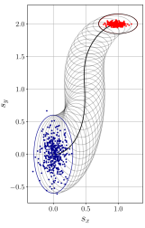
(a) SVGP Model

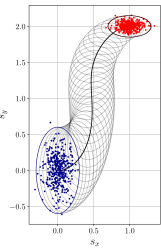
(b) Exact Model

Figure 1: Position ($s_{x}$, $s_{y}$) uncertainties. Blue: initial distribution. Red: target distribution. Black: actual terminal distribution. Gray: intermediate distributions. Solid black line: mean trajectory.

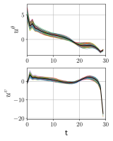
(a) SVGP Model

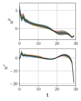
(b) Exact Model

Figure 2: Inputs ${\mathbf{u}}_{t}$. Solid black: mean input ${\boldsymbol{\nu}}_{t}$. Colored: inputs of Monte Carlo realizations.

(a) SVGP Model

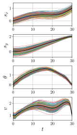
(b) Exact Model

Figure 3: States ${\mathbf{z}}_{t}$. Solid black: mean state ${\mathbf{z}}_{t}$. Colored: states of Monte Carlo realizations.

5 Conclusion

In this work, a greedy covariance steering algorithm that uses scalable Gaussian process predictive models for discrete-time stochastic nonlinear systems with unknown dynamics has been proposed. First, a non-parametric predictive model is learned from a set of training data points using stochastic variational Gaussian process regression. Then, a set of linearized covariance steering problems is solved and the mean and covariance of the closed-loop system is predicted using the unscented transform. This work has considered the case of perfect full-state information. However, more practical cases, such as that of incomplete information, where the states of the system have to be estimated from partial measurements, will be explored in the future by the authors.

References

- Bakolas (2016) Bakolas, E. (2016). Optimal covariance control for discrete-time stochastic linear systems subject to constraints. In IEEE CDC (2016), 1153–1158.
- Bakolas (2017) Bakolas, E. (2017). Covariance control for discrete-time stochastic linear systems with incomplete state information. In 2017 American Control Conference (ACC), 432–437.
- Bakolas (2018) Bakolas, E. (2018). Finite-horizon covariance control for discrete-time stochastic linear systems subject to input constraints. Automatica, 91, 61–68.
- Bakolas (2019) Bakolas, E. (2019). Dynamic output feedback control of the liouville equation for discrete-time siso linear systems. IEEE Transactions on Automatic Control, 64(10), 4268–4275.
- Bakolas and Tsolovikos (2020) Bakolas, E. and Tsolovikos, A. (2020). Greedy finite-horizon covariance steering for discrete-time stochastic nonlinear systems based on the unscented transform. In ACC (2020), 3595–3600.
- Caluya and Halder (2019) Caluya, K.F. and Halder, A. (2019). Finite horizon density control for static state feedback linearizable systems. arXiv preprint arXiv:1904.02272.
- Chen et al. (2016a) Chen, Y., Georgiou, T., and Pavon, M. (2016a). Optimal steering of a linear stochastic system to a final probability distribution, Part I. IEEE Trans. on Autom. Control, 61(5), 1158 – 1169.
- Chen et al. (2016b) Chen, Y., Georgiou, T., and Pavon, M. (2016b). Optimal steering of a linear stochastic system to a final probability distribution, Part II. IEEE Trans. Autom. Control, 61(5), 1170–1180.
- Gardner et al. (2018) Gardner, J.R., Pleiss, G., Bindel, D., Weinberger, K.Q., and Wilson, A.G. (2018). GPyTorch: Blackbox matrix-matrix gaussian process inference with GPU acceleration. arXiv preprint arXiv:1809.11165.
- Goldshtein and Tsiotras (2017) Goldshtein, M. and Tsiotras, P. (2017). Finite-horizon covariance control of linear time-varying systems. In IEEE CDC (2017), 3606–3611.
- Grigoriadis and Skelton (1997) Grigoriadis, K.M. and Skelton, R.E. (1997). Minimum-energy covariance controllers. Automatica, 33(4), 569–578.
- Grimes et al. (2006) Grimes, D.B., Chalodhorn, R., and Rao, R.P. (2006). Dynamic imitation in a humanoid robot through nonparametric probabilistic inference. In Robotics: science and systems, 199–206. Cambridge, MA.
- Hensman et al. (2013) Hensman, J., Fusi, N., and Lawrence, N.D. (2013). Gaussian processes for big data. arXiv preprint arXiv:1309.6835.
- Hoffman et al. (2013) Hoffman, M.D., Blei, D.M., Wang, C., and Paisley, J. (2013). Stochastic variational inference. Journal of Machine Learning Research, 14(5).
- Hotz and Skelton (1987) Hotz, A. and Skelton, R.E. (1987). Covariance control theory. Int. J. Control, 16(1), 13–32.
- Julier and Uhlmann (2004) Julier, S.J. and Uhlmann, J.K. (2004). Unscented filtering and nonlinear estimation. Proc. IEEE, 92(3), 401–422.
- Julier (2002) Julier, S.J. (2002). The scaled unscented transformation. In ACC (2002), volume 6, 4555–4559. IEEE.
- Kingma and Ba (2014) Kingma, D.P. and Ba, J. (2014). Adam: A method for stochastic optimization. arXiv preprint arXiv:1412.6980.
- Ko and Fox (2009) Ko, J. and Fox, D. (2009). GP-Bayesfilters: Bayesian filtering using gaussian process prediction and observation models. Autonomous Robots, 27(1), 75–90.
- Ko et al. (2007a) Ko, J., Klein, D.J., Fox, D., and Haehnel, D. (2007a). Gaussian processes and reinforcement learning for identification and control of an autonomous blimp. In ICRA (2007), 742–747.
- Ko et al. (2007b) Ko, J., Klein, D.J., Fox, D., and Haehnel, D. (2007b). GP-UKF: Unscented kalman filters with gaussian process prediction and observation models. In IROS (2007), 1901–1907.
- Mesbah et al. (2014) Mesbah, A., Streif, S., Findeisen, R., and Braatz, R.D. (2014). Stochastic nonlinear model predictive control with probabilistic constraints. In ACC (2014), 2413–2419.
- Mukadam et al. (2016) Mukadam, M., Yan, X., and Boots, B. (2016). Gaussian process motion planning. In ICRA (2016), 9–15.
- Pan and Theodorou (2014) Pan, Y. and Theodorou, E. (2014). Probabilistic differential dynamic programming. In NIPS (2014), 1907–1915.
- Pan and Theodorou (2015) Pan, Y. and Theodorou, E.A. (2015). Data-driven differential dynamic programming using gaussian processes. In ACC (2015), 4467–4472.
- Paszke et al. (2017) Paszke, A., Gross, S., Chintala, S., Chanan, G., Yang, E., DeVito, Z., Lin, Z., Desmaison, A., Antiga, L., and Lerer, A. (2017). Automatic differentiation in PyTorch.
- Quinonero-Candela and Rasmussen (2005) Quinonero-Candela, J. and Rasmussen, C.E. (2005). A unifying view of sparse approximate gaussian process regression. The Journal of Machine Learning Research, 6, 1939–1959.
- Rasmussen (2003) Rasmussen, C.E. (2003). Gaussian processes in machine learning. In Summer School on Machine Learning, 63–71. Springer.
- Ridderhof et al. (2019) Ridderhof, J., Okamoto, K., and Tsiotras, P. (2019). Nonlinear uncertainty control with iterative covariance steering. In CDC (2020), 3484–3490.
- Sehr and Bitmead (2017) Sehr, M.A. and Bitmead, R.R. (2017). Particle model predictive control: Tractable stochastic nonlinear output-feedback MPC. In 20th IFAC World Congress, 15361 – 15366.
- Titsias (2009) Titsias, M. (2009). Variational learning of inducing variables in sparse gaussian processes. In Artificial intelligence and statistics, 567–574. PMLR.
- Wan and Van Der Merwe (2000) Wan, E.A. and Van Der Merwe, R. (2000). The unscented Kalman filter for nonlinear estimation. In Proceedings of the IEEE 2000 Adaptive Systems for Signal Processing, Communications, and Control Symposium, 153–158.
- Xu and Skelton (1992) Xu, J.H. and Skelton, R.E. (1992). An improved covariance assignment theory for discrete systems. IEEE Trans. Autom. Control, 37(10), 1588–1591.