XDA: Accurate, Robust Disassembly with
Transfer Learning

Abstract

Accurate and robust disassembly of stripped binaries is challenging. The root of the difficulty is that high-level structures, such as instruction and function boundaries, are absent in stripped binaries and must be recovered based on incomplete information. Current disassembly approaches rely on heuristics or simple pattern matching to approximate the recovery, but these methods are often inaccurate and brittle, especially across different compiler optimizations.

We present XDA, a transfer-learning-based disassembly framework that learns different contextual dependencies present in machine code and transfers this knowledge for accurate and robust disassembly. We design a self-supervised learning task motivated by masked Language Modeling to learn interactions among byte sequences in binaries. The outputs from this task are byte embeddings that encode sophisticated contextual dependencies between input binaries’ byte tokens, which can then be finetuned for downstream disassembly tasks.

We evaluate XDA’s performance on two disassembly tasks, recovering function boundaries and assembly instructions, on a collection of 3,121 binaries taken from SPEC CPU2017, SPEC CPU2006, and the BAP corpus. The binaries are compiled by GCC, ICC, and MSVC on x86/x64 Windows and Linux platforms over 4 optimization levels. XDA achieves 99.0% and 99.7% F1 score at recovering function boundaries and instructions, respectively, surpassing the previous state-of-the-art on both tasks. It also maintains speed on par with the fastest ML-based approach and is up to 38$\times$ faster than hand-written disassemblers like IDA Pro. We release the code of XDA at https://github.com/CUMLSec/XDA.

I Introduction

Disassembly is the backbone of many binary analysis tasks, such as malware analysis, reverse engineering, retrofitting control-flow integrity defenses, binary rewriting, and binary instrumentation [20, 51, 55, 50, 40]. Binary analysis relies on disassembly to recover higher-level constructs such as assembly instructions and function boundaries from machine code.

Disassembly is difficult because high-level information from symbol tables and source code are absent in stripped binaries. This information is either discarded during compilation or stripped before distribution to decrease program size or deter reverse engineering. Therefore, disassemblers must approximate the recovery of higher-level constructs from incomplete information. Complex assembly constructs such as inline data and tail calls, further complicate disassembly.

Traditional approaches to this problem rely on handcrafted heuristics to guide the recovery, but these methods are inaccurate and brittle [58, 7, 5]. For example, many popular disassemblers, like IDA Pro and Ghidra, recover assembly instructions by recursively following direct control flow transfers (e.g., call 0x2ed4). Similarly, they recover function boundaries by looking for known instruction patterns. These heuristics-based methods are insufficient – prior research has shown that IDA Pro misidentifies up to 58% of function boundaries [7] and 4% of assembly instructions [4] in optimized binaries. Furthermore, many heuristics for detecting functions require continual manual maintenance of large databases to adapt to code and compiler changes [7]: IDA Pro’s current database for identifying common library functions is over 41MB in size, and Ghidra’s is over 179MB.

Previous research has explored using Machine Learning (ML) to address these challenges. The resulting models surpassed the accuracy of traditional disassemblers at both recovering assembly instructions [58] and function boundaries [7, 48], and are easier to maintain. However, current ML-based approaches still face two critical challenges:

Accuracy. Recent research has shown that previous ML-based methods are likely not as accurate as reported [5]. This is because their accuracies were inadvertently measured on testing data with significant overlap with training data, and therefore their performance may not generalize to real-world binaries. More concretely, Andriesse et al. [5] showed that the F1 score of ByteWeight [7] degrades from the reported 97% to 65% when evaluated on a dataset without overlap.

Robustness. The current most accurate ML approach for recovering function boundaries, bidirectional Recurrent Neural Net (bi-RNN) [48], is not robust to compiler optimization changes (see Section VII-B). Similar concerns have also been raised by Wang et al. [56], who proposed a more robust method by combining ML with symbolic execution. However, this method does not scale well to larger binaries.

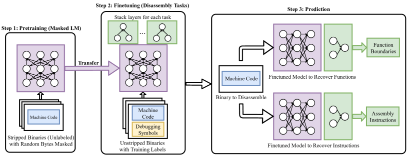
Figure 1: The workflow of XDA. We first pretrain the model with the masked LM task, and then finetune the pretrained model with new stacked NN layers for disassembly tasks. Finetuning updates both the pretrained model and the stacked layers. During inference, the finetuned models takes the binary and output disassembly information, depending on the finetuned tasks.

In this paper, we present XDA (Xfer-learning DisAssembler), a new ML-based disassembly framework that uses transfer learning to address these challenges. We train and evaluate XDA on 3,121 binaries, and separate the testing and training data such that they have minimal overlap (less than 3%). We show that XDA outperforms all state-of-the-art tools in accuracy at recovering function boundaries and assembly instructions, and is robust to changes in compiler optimization. Additionally, XDA’s speed is on par with the fastest tools.

Our key insight is to teach the ML model general dependencies between bytes in machine code before training it to perform specific disassembly tasks – we transfer its learned knowledge of these byte dependencies to tackling disassembly. Intuitively, we first teach our model to read and gain a basic understanding of machine code and then teach it to solve a disassembly task. We achieve this by splitting our training into two stages, as shown in Figure 1. In the first stage, we pretrain our model using masked Language Modeling (masked LM) to teach it the byte dependencies of x86/x64 machine code. In the second stage, we finetune our model to leverage its knowledge of byte dependencies to solve a specific disassembly task accurately and robustly.

The masked LM task asks the model to predict randomly masked bytes, which requires the model to produce missing bytes given the context. This design compels the model to learn dependencies between the masked byte and surrounding bytes, teaching the model a basic understanding of machine code semantics. As we will show in Section VII, this understanding improves not only the model’s accuracy but also its robustness to compiler and optimization changes. In contrast, previous ML approaches rely on superficial patterns, such as function prologues, which limits their accuracy and robustness when such patterns are absent or changed. An additional benefit is that the masked byte prediction task does not require labeled data. Therefore, XDA can be further trained and improved using stripped binaries found in the wild.

We give some intuition on why the masked LM task is helpful for disassembly. Consider a function that uses 0x28 bytes of stack space for local variables. To allocate this space, the function uses sub rsp,0x28 to decrement the stack register by 0x28 bytes. Now assume the byte 0x28 is masked, like so: sub rsp,??. To predict the value of this masked byte, our pretrained model learns to search for the corresponding stack deallocation instruction (add rsp,0x28) and read its value (see Section VIII-B for more details). Since stack allocation/deallocation often occurs near the start/end of a function, the knowledge of this dependency is a helpful feature for identifying function boundaries. Such scenarios that naturally occur in predicting randomly masked bytes, in sum, teaches the model a powerful, general understanding of machine code semantics that helps disassembly.

To evaluate XDA’s performance, we test it on 3,121 Linux and Windows x86/x64 binaries taken from the SPEC CPU2017 [14], SPEC CPU2006 [15] benchmark suites and the BAP corpus [7]. These binaries are compiled using the GNU Compiler Collection (GCC), Intel C++ Compiler (ICC), and Microsoft Visual C++ (MSVC) over 4 optimization levels (O0-O3 for GCC and ICC, O1, O2, Od, Ox for MSVC). We choose two popular disassembly tasks, recovering function boundaries and assembly instructions, to test our model’s performance, but XDA can be easily finetuned for other disassembly and binary analysis tasks. Across these binaries, XDA achieves 99% F1 score at recovering function boundaries, 17.2% higher than the second-best tool. XDA also achieves a 99.7% F1 score at recovering assembly instructions. Furthermore, XDA’s underlying neural architecture is highly parallelizable and efficient, running up to 38$\times$ faster than hand-written disassemblers like IDA Pro.

We also evaluate the robustness of XDA to the changes of compiler optimizations. XDA achieves at least 98.5% F1 score at recovering function boundaries in highly optimized binaries, even when it is only finetuned on unoptimized binaries.

We make the following contributions.

• We propose a new approach to disassembly using a two-step transfer learning paradigm: we first pretrain the model to teach it a basic understanding of machine code, then finetune it to solve disassembly tasks.

• We demonstrate that masked LM is an effective pretraining task for disassembly because it compels the model to learn machine code semantics (Section III). We then show how this semantic knowledge can be leveraged in finetuning to accurately and robustly solve two popular disassembly tasks, recovering function boundaries and assembly instructions.

• We implement XDA and evaluate it on a collection of x86/x64 binaries from the SPEC CPU2017, SPEC CPU2006, and BAP dataset on both the Windows and Linux platforms (Sections VI and VII). The binaries are compiled by GCC, ICC, and MSVC over 4 optimization levels. Even when the pretraining, finetuning, and testing datasets are strictly separated, XDA achieves an average F1 score of 99.0% at recovering function boundaries, outperforming the state-of-the-art by 17.2%, and an average F1 score of 99.7% at recovering assembly instructions. We open-source our implementation at https://github.com/CUMLSec/XDA.

II Background

We briefly overview the two disassembly tasks we tackle, recovering function boundaries and assembly instructions, two fundamental building blocks in binary analysis research [4]. We then describe their challenges faced by existing tools using real-world examples.

The definition of disassembly can be ambiguous, as some authors refer only to the process of recovering instructions from binaries [36, 8, 58]. We adopt the more inclusive interpretation defined by Andriesse et al. [4, 5]: Disassembly is the process of recovering higher-level program constructs lost during compilation, such as assembly instructions, function boundaries, function signatures, and control flow graphs.

Most disassembly tools recover these constructs via static analysis, because dynamic analysis has large runtime overheads and struggles to achieve high completeness in complex programs. Therefore, we also limit our methods to operate on information acquirable without executing the program.

II-A Recovering Function Boundaries

The task of recovering function boundaries consists of identifying the matched start and end addresses of each function in a stripped binary. We inherit the formal definition of this task by Bao et al. [7]: given a binary that contains a set of functions $F=\{f_{1},f_{2},...,f_{n}\}$, recover a set of function start and end address pairs $S=\{(s_{1},e_{1}),(s_{2},e_{2}),...,(s_{n},e_{n})\}$ such that for all $f_{i}\in F,\ s_{i}$ is the address of the first byte of $f_{i}$ and $e_{i}$ marks the end of $f_{i}$ (the first byte not contained in $f_{i}$).

Recovering function boundaries from stripped binaries is one of the most challenging disassembly tasks [4, 7, 32, 26, 54, 49, 50, 18]. Functions are source-level constructs but decay to simple control-flow transfer at the machine code level, and symbol tables containing function information are removed. Compiler optimizations exacerbate the problem by removing indicative structures such as function prologues. For disassemblers operating on recovered assembly instructions instead of machine code, an additional concern is functions whose instructions are not recovered cannot be identified.

II-B Recovering Assembly Instructions

The task of recovering assembly instructions consists of identifying the bounds of each individual assembly instruction within the code sections of a stripped binary.

The main difficulty of recovering assembly instructions comes from distinguishing inline data from code via static analysis [36]. Architectures like x86 and x64 have variable-length instructions and do not make syntactic distinctions between inline data and code [8, 58]. However, compilers such as MSVC interleave data with code for code efficiency. In the worst case, the only difference between data and code at the machine code level is that code bytes are reachable at runtime. Therefore, perfectly recovering assembly instructions from x86 and x64 binaries is undecidable [58, 57]. Mistakenly parsing a data byte as the start of a multi-byte instruction can desynchronize the disassembled instruction stream alignment, propagating the error forward [4].

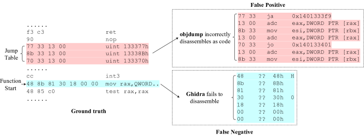
Figure 2: Real-world example that fails objdump and Ghidra. The ground truth assembly instructions include (1) a jump table in the code section that objdump cannot identify, and (2) a function reached via an indirect control flow transfer that Ghidra cannot statically determine.

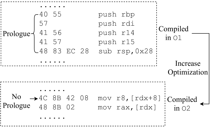
Figure 3: Both IDA Pro and bi-RNN recognized this function when it was not optimized (O1), but failed to recognize it in higher optimization (O2) when the function prologue is optimized away.

II-C Challenging Cases

We use code snippets from Vim 8.2 compiled by MSVC 2019 to demonstrate some challenges faced by heuristic-based approaches. This serves primarily as a motivating example. For a more thorough listing of challenging disassembly cases, we refer interested readers to Andriesse et al. [4].

Traditional disassemblers rely on heuristics to recover function boundaries and assembly instructions, requiring data such as control flow information and function prologues/epilogues, which restricts their accuracy and robustness. For example, Figure 2 shows the linear disassembler objdump and the recursive traversal disassembler Ghidra failing to disassemble a section of code. objdump misinterpreted a jump table as instructions, whereas Ghidra missed an entire function of code. Similarly, in Figure 3 IDA Pro and bi-RNN fail to recognize a function when the compiler optimization is increased, removing the function prologue.

In contrast, XDA correctly recovers all instructions and functions in this code. The key to this success is XDA’s transfer learning approach, which enables it to capture general patterns that match real program dependencies and semantics. We provide the intuition behind this in the following section.

III Overview of Our Approach

We have shown XDA’s workflow of pretraining and finetuning in Figure 1. In this section, we describe how the pretraining task, masked LM, compels the model to learn machine code dependencies that could support many downstream disassembly tasks. Although formally proving such claims remains an open question [6], we sketch two intuitive cases below to motivate why predicting masked bytes teaches the model machine code semantics that helps disassembly. We include the more complete details in Sections VIII-A.

Recall the definition of the masked LM pretraining task: given a byte sequence, we mask out some random bytes, and train the model to predict the masked bytes using the non-masked bytes. The non-masked bytes are known as the contextual information. We use two examples to show that pretraining with masked LM allows a model to thoroughly understand properties of machine code, aiding recovery of function boundaries and assembly instructions.

Masking local variable allocation. Consider the code snippet in Figure 3, where we mask four bytes (48 83 ec 28), representing sub rsp,0x28 that decrements the stack pointer to allocate 40 bytes for local variables. Unlike the example described in Section I, the model does not have access to the corresponding stack deallocation instruction. We found that our model still correctly predicts the four bytes with high confidence, which implies the model understands the semantics of stack allocation and can deduce the space required by local variables by looking at the surrounding bytes in the function body. Besides, the understanding of such semantics can significantly help in recovering function boundaries, because the function prologue strongly indicates a function start. Section VII-E shows pretraining with such tasks improves the results by 50% at recovering function boundaries.

Masking jump table entries. Now consider the jump table example in Figure 2, where we mask out the jump table entry 77 33 13 00. We find that our model correctly predicts the four bytes with high confidence, which indicates it learns to distinguish inline data from code. For example, if it treats the masked bytes as instructions (like those disassembled by objdump shown on the right), it is highly unlikely for the model to predict 77 33 (the ja instruction) right after the instructions ret; nop. The reason is that compiler-generated byte code (XDA’s training data) rarely places a conditional jump like ja, which depends on flags set by cmp or test, after an nop. Therefore, the model should understand the masked bytes are part of the inline data section, which should be similar to the following (as opposed to the preceding) bytes corresponding to other jump table entries.

To confirm that the model is not simply memorizing the byte order in Vim, we remove all Vim binaries (shown in Figures 2 and 3) from the training set. Therefore, the model’s high accuracy strongly indicates that the semantics described above is captured in the pretraining process.

IV Threat Model

Robustness. We focus on binaries generated by standard compilers. Like other disassemblers, we do not aim to be robust in the presence of arbitrarily obfuscated code. Instead, we aim to be robust against compiler changes, which often occur due to improvements in optimization. In Section VII-B, we evaluate the robustness of our model by testing it on binaries compiled on higher optimization levels than the model is trained on.

False positives and negatives. Like most disassemblers, we assume a small number of false positives and negatives can be tolerated. Certain use cases in binary rewriting require recovered instructions to contain strictly no false positives or no false negatives; we do not enforce these requirements.

V Methodology

We describe the design specifics of XDA, including the key components of the architecture and workflow of pretraining and finetuning. We then elaborate on the technical details in the following subsections.

General design. Figure 4 shows the simplified architecture of XDA and bi-RNN [48] and their example input-output. It highlights XDA’s two key design differences with a typical ML-based technique, bi-RNN [48]. The first is the employment of a pretraining task. As discussed in Section III, this design encourages the model to learn machine code contextual dependencies helpful for many binary analysis tasks.

Second, we employ self-attention layers [53] in the model to compute information flow between every pair of bytes. Specifically, we follow the encoder architecture in Transformer [53] with several modifications (Section V-A). This design is shown more capable than the sequential connections in RNNs in capturing long-range dependencies between distant bytes. As we will show in Section VIII, the model often needs to learn and understand long-range dependencies in the binaries to recover functions boundaries and instructions accurately.

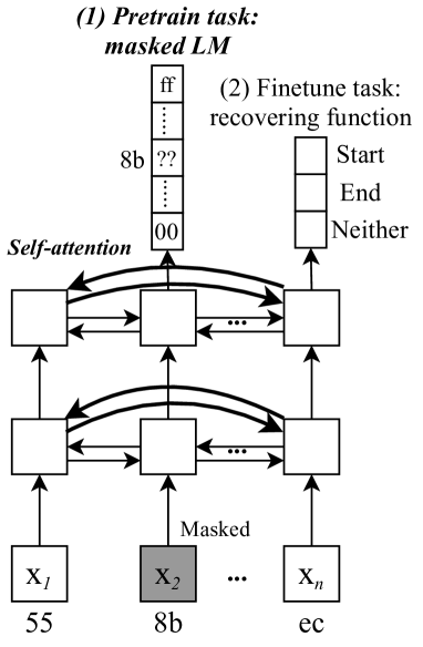
(a) XDA architecture

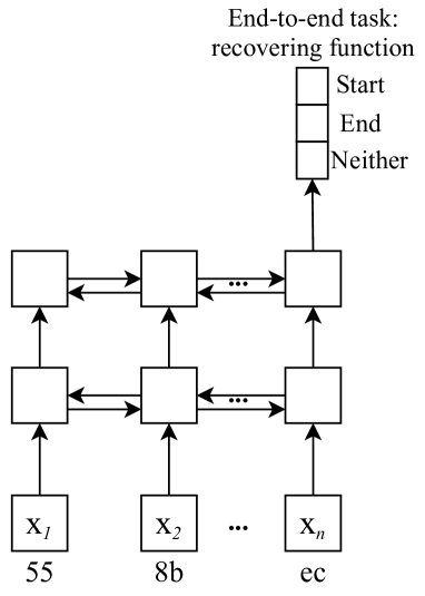
(b) bi-RNN architecture [48]

Figure 4: Architectural differences between XDA and bi-RNN used by Shin et al. [48]. Two key distinguishing components of XDA are: (1) the pretraining (masked LM) steps, and (2) self-attention connections between arbitrary tokens instead of only between neighbors.

Input representation. Formally, we define the input $x$ as a sequence of byte tokens of size $n$: $x=${0x00, …, 0xff}ⁿ. Each input byte $x_{i}\in x$ is represented as a one-hot encoded vector (e.g., a3 is encoded as a 256-dimensional vector with all 0s but single 1 at position 163). Besides 256 possible byte values, the input vocabulary has 5 additional reserved tokens (i.e., padding <PAD>, start-of-sequence <S> and end-of-sequence </S>, unknown <UNK>, and mask <MASK>). Also, note that here we do not put constraints on $n$. For example, the byte sequences can span multiple binary programs, or include only a subset of byte sequence within a single binary.

Pretraining task. We pretrain the model using the masked LM objective. Formally, for each byte sequence $x_{1},...,x_{n}$ in a given training set, we mask out some percentage of byte tokens in each sequence randomly (see Section V-C for details). The masked byte tokens are replaced by the mask tokens (<MASK>).

Let $mask(x_{i})$ denote the output of applying the mask on the $i$-th byte in $x$ and $mpos$ a set of masked byte’s positions in $x$. The model to be pretrained, $f_{p}$, will take as input the byte sequence with random bytes masked: $(x_{1},...,mask(x_{i}),...,x_{n}),i\in mpos$, and predicts the byte values of the masked tokens: $\{\hat{x}_{i}|i\in mpos\}=f_{p}(x_{1},...,mask(x_{i}),...,x_{n})$. Let $f_{p}$ be parameterized by $\theta$ ($f_{p}(-;\theta)$), the objective of training $f_{p}$ is thus to search for $\theta$ that minimizes the cross entropy loss between the predicted masked bytes and the actual bytes. For ease of exposition, we omit summation over all samples in the training set.

$$\centering\operatorname*{arg\,min}_{\theta}\sum\limits_{i=1}^{|mpos|}-x_{i}\log(\hat{x}_{i})\@add@centering$$ (1)

While the pretrained model’s input and output are one-hot encoded byte tokens, all of its intermediate layers operate on the embedding vectors. For each byte $x_{i}$, let $E_{1,i}$ denote its embedding after $1$-st layer, the embeddings produced by the $l$-th layer of the model is $E_{l}=(E_{l,1},...,E_{l,n})$. Let layer $l$ be the $f_{p}$’s last layer; $E_{l}$ is not the actual outputs of $f_{p}$, as $f_{p}$ will take $E_{l}$ and stack a classification layer (e.g., softmax) to predict the value of the byte tokens. Given the produced embeddings $E_{l}$, we define finetuning tasks in the following.

Finetuning tasks. Given a sequence of embedding vectors produced by the pretrained model $E_{l}=(E_{l,1},E_{l,2},...,E_{l,n})$, the corresponding ground truth $y$ in our finetuning task is a sequence of labels of same length $n$: $\{y_{i}|y_{i}\in C_{y}\}^{n}$, where $C_{y}$ denote the set of all possible class labels of $y$. Each byte embedding $E_{l,i}$ will be mapped to a label $y_{i}$.

Let $f_{t}$ denote the model to be finetuned. It takes as input each byte embedding $E_{l,i}$, and predicts the label $\hat{y_{i}}$, where $\hat{y_{i}}=f_{t}(E_{l,i})$. Now let $f_{t}$ be parameterized by $\theta$: $f_{t}(E_{l,i};\theta)$, the objective of training $f_{t}$ is thus to search for $\theta$ that minimizes the cross entropy between the predicted labels of all byte embeddings and their actual labels:

$$\centering\operatorname*{arg\,min}_{\theta}\sum\limits_{i=1}^{n}-y_{i}\log(\hat{y_{i}})\@add@centering$$ (2)

As both $f_{p}$ and $f_{t}$ in our setting are neural networks, solving Equations 1 and 2 can be efficiently guided by gradient descent via backpropagation. The gradient can flow through both $\theta$s in $f_{p}$ and $f_{t}$ during finetuning, as $f_{p}$ is also part of the computation of $\hat{y}^{(i)}_{j}$. Thus, the pretrained parameters in $f_{p}$ also get updated during finetuning to adjust for specific downstream tasks.

As a concrete example, consider recovering function boundaries. The possible class labels $C_{y}=\{S,E,N\}$ denote the function start ($S$), end ($E$), and neither ($N$). $f_{t}$ takes each byte embedding as input and produces the probability distributions of three possible labels, where the predicted label will be the one with the highest probability. This is illustrated in Figure 4a.

V-A Masked Language Model on Binaries

As illustrated in Figure 4a, the forward pass within the XDA’s architecture consists of the following steps.

First, XDA embeds the one-hot vectors of each input byte (both masked and not masked) as a fixed-dimension embedding vector. What is not shown in Figure 4a is that XDA also computes the positional embeddings, which encode the position of each byte within the sequence as another vector that has the same size with the byte embeddings. The rationale of using the positional embeddings is to assign distinctive meanings to the same byte tokens appearing in different locations within the sequence. Note that in recurrent-based networks, such spacial relationship is naturally encoded as the information flow follows the order in the input sequence [53]. Two embeddings (i.e., byte embeddings and positional embeddings) are then combined as the actual embeddings of input for the next layer.

XDA then employs multi-head self-attention to update the embeddings. At each self-attention layer, each embedding combines itself with a weighted sum of all other embeddings, where the attention strength determines the weight.

Finally, XDA predicts the byte values of masked bytes based on its updated embeddings in the last layer. To this end, XDA stacks a 2-layer fully-connected network with the output dimension equal to the input vocabulary size. The updated embedding here is known as contextualized embedding [34, 35, 41, 42, 17] as it takes into account the information of other byte tokens within the sequence.

In the following, we elaborate on the key concepts described above. We will use the same notations defined in Section V wherever they are applicable.

Byte position embeddings. The position of each input byte is critical for inferring binary semantics. Unlike natural language, where swapping two words can roughly preserve the same semantic meaning, swapping two bytes can significantly change the instructions. Therefore, we use the learned positional embedding $E_{pos}$ (embedding matrix itself is learnable) and stack a feedforward network $F$ with one hidden layer to combine $E_{pos}$ with byte embeddings $E_{byte}$. Specifically, let $E_{byte}(x)$ denote applying the embedding to the one-hot encoded byte token $x_{i}$, and let $E_{pos}(i)$ denote applying the learned positional embedding to $x_{i}$’s position $i$, we have: $E_{1,i}=F(concat(E_{byte}(x_{i}),E_{pos}(i)))$. As defined in Section V, $E_{1,i}$ here refers to the embedding of $x_{i}$ in the 1st attention layer.

Multi-head self-attention. Given the embeddings of all bytes in $k$-th layer, $(E_{k,1},...,E_{k,n})$, the core operations of a single attention head in self-attention layer is to update each embedding by the following steps.

First, each embedding $E_{k,i}$ will get mapped to three values following query-key-value computation: $query_{i}=f_{query}(W_{query};E_{k,i})$, $key_{i}=f_{key}(W_{key};E_{k,i})$, $value_{i}=f_{value}(W_{value};E_{k,i})$. Here $f_{query}$, $f_{key}$, and $f_{value}$ are affine transformation functions (i.e., a fully-connected layer) parameterized by $W_{query}$, $W_{key}$, and $W_{value}$, respectively.

Each embedding $E_{k,i}$ then computes attention score $s_{ij}$ with all other embeddings $E_{k,\{j|j\neq i\}}$ by taking the dot product between the $E_{k,i}$’s query $query_{i}$ and $E_{k,j}$’s key $key_{j}$: $s_{ij}=query_{i}\cdot key_{j}$. Intuitively, attention scores $s$ for all pairs will end up as a square matrix, where each cell $s_{ij}$ indicates how much attention $E_{k,i}$ should pay to $E_{k,j}$ when updating itself. We then divide every row of $s$ by $\sqrt{d_{emb}}$ (the dimension of the embedding vectors) and scale it by softmax to ensure them sum up to 1: $s^{\prime}_{ij}=\frac{\exp(s_{ij})}{\sum^{n}_{j=1}\exp(s_{ij})}$ The scaled attention score $s^{\prime}_{ij}$ will be multiplied with $value_{j}$ and summed up: $E^{h}_{k+1,i}=\sum^{n}_{j=1}s^{\prime}_{ij}v_{j}$

Here $h$ in $E^{h}_{k+1,i}$ denote the updated embeddings belong to attention head $h$. Assume we have total $H$ attention heads, the updated embeddings will finally go through an 2-layer feedforward network $f_{out}$ parameterized by $W_{out}$ with skip connections [27] to update embeddings from all heads: $E_{k+1,i}=f_{out}(concat(E^{0}_{k+1,i},...,E^{H}_{k+1,i});W_{out})$.

Contextualized embeddings. The multi-layer attention mechanism updates its embeddings iteratively up to the last layer. The embeddings at each self-attention layer are known as contextualized (or context-aware) embeddings. One significant feature of contextualized embeddings is that the underlying meaning of each embedding depends on the other tokens in the input sequence. So the embeddings for the same byte token can be different if the byte is in a different context (surrounded by different bytes). This is in contrast with static embeddings (e.g., word2vec [35]) commonly used by other related works (e.g., learn binary embeddings [21, 19]), where a byte token is always assigned to the same fixed embedding regardless of the changed context (i.e., surrounding bytes).

V-B Distilling the Learned Semantics

The examples in Section III motivate how pretraining on masked LM task encourages learning semantics. However, they are all implicitly embedded in the weight parameters of the underlying neural network. To distill the learned semantics for different downstream tasks, we leverage the contextualized embeddings produced by the pretrained model’s last layer and stack a simple 2-layer multi-layer perceptron (MLP) for prediction. Explicitly, for each embedding $E_{l,i}$ in the last layer, we fix the network to perform the following computation: $MLP(E_{l,i})=softmax(tanh(E_{l,i}\cdot W_{1})\cdot W_{2})$. Here $W_{1}\in\mathbb{R}^{d_{emb}\times d_{emb}}$ and $W_{2}\in\mathbb{R}^{d_{emb}\times|C_{y}|}$ where $|C_{y}|$ is the number of output classes (defined in Section V). Note that we apply $MLP$ to each byte embedding. Therefore, the output of $MLP$ is of shape $\mathbb{R}^{n\times|C_{y}|}$, where $n$ is the length of the input sequence.

V-C Masking Input Bytes

For each input sequence in pretraining, we choose 20% random bytes to mask. Among the chosen bytes, we select 50% of them to be replaced by the special token <MASK>. For the remaining 50% of the masked bytes, we replace with random bytes in the vocabulary {0x00, …, 0xff}. The reason of not replacing all chosen bytes by <MASK> is that, in the finetuning task, there is no such token. Therefore, we try to prevent the model from discovering any spurious meanings of the <MASK> token itself, but encourage the model to focus on using the context to predict the masked tokens.

For the same input sequences at different epoch, we re-randomize the bytes to mask instead of fixing the same set of masked bytes throughout different epochs. Therefore, we implement a dynamic masking scheme and do not apply masking in the data preprocessing stage.

VI Implementation and Experimental Setup

We build the learning module of XDA in PyTorch 1.4.0 with CUDA 10.1 and CUDNN 7.6.3. We implement the self-attention architecture using Fairseq toolkit [39]. We run the training and inference of our models on a Linux server running Ubuntu 18.04, with an Intel Xeon E5-2623 at 2.60GHz with 16 virtual cores including hyperthreading, 256GB RAM, and 3 Nvidia GTX 1080-Ti GPUs.

Datasets. Table I summarizes the datasets we use for training and evaluating XDA. The first dataset is SPEC CPU2017 [15], the updated version of SPEC CPU benchmarks. It includes 39 C/C++/Fortran compute-intensive programs. We compile each program using 2 compilers, GCC-9.2 and MSVC 2019 on Linux and Windows, respectively. Each compiler compiles the program on 2 ISAs (x86 and x64) with respective 4 optimization levels (e.g., O1, O2, Ox, Od for MSVC, and O0-O3 for GCC/ICC). Due to various constraints (e.g., some speed testing programs do not support x86), we cannot compile all programs using all optimization flags. In total, we have 588 compiled binaries for SPEC CPU2017.

The second dataset is SPEC CPU2006 [15], the former generation of SPEC benchmarks. It includes 19 C/C++/Fortran programs. We follow the same configurations as Andriesse et al. [4] to compile SPEC CPU2006 so that we can easily obtain the ground truth for function and instruction boundaries. For example, we use the legacy GCC-5.1.1 to compile on Linux platforms. However, the Windows compilation and configuration are not available and no longer maintained after we have contacted the authors. Therefore, we use MSVC 2008 on a Windows XP virtual machine to compile the binaries for the Windows platform. To compensate for relatively small number of available binaries comparing to SPEC CPU2017, we turn on one extra optimization flag in GCC (Os), just to enlarge the pretraining dataset and introduce more byte patterns. As the default installations of GCC-5.1.1 and MSVC 2008 cannot compile certain legacy programs in SPEC CPU2006, we have in total 333 compiled binaries.

The third dataset is from BAP corpora [7]. It includes 2,200 compiled binaries where 136 popular open-source programs (e.g., vim) are on Windows platform, and the remaining 2,064 ELF binaries (from coreutils, binutils, and findutils packages) are compiled on Linux platform. Both sets are further divided equally into x86 and x64 binaries.

TABLE I: General statistics of all binaries and performance of XDA on all binaries (discussed in Section VII-A). The byte sequences are of length 512 (see Appendix Section -A). We use 10% of the binaries for training (in finetuning) across all datasets and the corresponding train-test overlap rate is shown in each row.

Dataset	Total # Binaries	Platform	Compiler	ISA	# Binaries	# Bytes	# Byte Sequences	Train-test Overlap
SPEC 2017	588	Linux	GCC-9.2	x86	120	198,019,576	386,757	0.001%
				x64	224	464,906,401	908,021	0.2%
		Windows	MSVC-2019	x86	88	175,057,814	341,910	0.93%
				x64	156	955,201,152	1,865,628	0.97%
SPEC 2006	333	Linux	GCC-5.1.1	x86	90	55,637,428	108,667	0.002%
				x64	95	74,006,029	144,543	0%
		Windows	MSVC-2019	x86	76	40,417,016	78,940	0.36%
				x64	72	48,403,456	94,538	0.21%
BAP	2,200	Linux	GCC-4.7.2 & ICC-14.0.1	x86	1,032	138,547,936	270,602	1%
				x64	1,032	145,544,012	284,266	1.1%
		Windows	MSVC-2010 & 2012 & 2013	x86	68	29,093,888	56,824	0.4%
				x64	68	33,351,168	65,139	2.3%

Baselines. We use IDA Pro v7.4 [47], Ghidra v9.1 [2], and objdump as baselines. We also compare XDA with the other two research prototypes that achieve state-of-the-art results on recovering function boundaries. The first one is Nucleus [5], which is based on the control-flow analysis. The second one is from Shin et al. [48], who designed a bi-RNN [48] to recover function boundaries. Since Shin et al. did not release their source code, we re-implement bi-RNN in PyTorch following the same setup described in their paper. Specifically, we adopt the 2-layer architecture with 16 hidden layer size, which reportedly achieves the best result.

Label collection. We collect the ground truth labels for function boundaries and assembly instructions using the debug symbols and source code of the binaries. (1) To get function boundaries for Windows binaries, we parse PDB files using Dia2dump [33]. For Linux binaries, we parse DWARF information using the pyelftools [9]. Like Bao et al. [7] and many disassemblers, we do not count thunks in Windows binaries and trampolines in the .plt section of Linux binaries as functions. We remove thunks and trampolines from the outputs of function recovery tools that count them as functions, to ensure that they are not inadvertently seen as false positives. (2) To get assembly instructions, we collect instruction boundaries as our ground truth, rather than the instructions themselves. This allows us to modularize the design of our model. Given the instruction boundaries, we can then deterministically map the bytes in each boundary to their corresponding instruction. To collect the instruction boundaries, we use source-level information to guide a linear disassembler to get the labels for most bytes, and then manually analyze the remaining bytes [4]. The linear disassembler we use is the Capstone library [43].

Metrics. Both tasks (i.e., recovering functions and instructions) have the imbalanced label problem. For example, the number of function boundaries (both start and end) in the SPEC CPU2006 dataset accounts for only 1.05% of the total number of bytes. A predictor that always outputs “not boundary” can achieve a 98.95% accuracy. Therefore, we use alternative metrics, described in the following.

Precision, recall, F1 score. We use precision ($P$), recall ($R$), and $F1$ score to measure the actual performance of XDA and all other tools. Consider recovering function boundaries. Let $TP$ (true positive) denote the number of correctly predicted (e.g., function) boundaries, $FP$ denote the number of incorrectly predicted boundaries, $FN$ denote the number of incorrectly predicted not-boundaries, and $TN$ denote the number of correctly predicted non-boundaries. $P=TP/(TP+FP)$, $R=TP/(TP+FN)$, and $F1=2\cdot P\cdot R/(P+R)$.

Perplexity. We use perplexity (PPL) to evaluate the masked LM pretraining task, which intuitively measures how “confused” the model is about the masked bytes being equal to the ground truth bytes. The less confused is the model, the smaller the perplexity. Specifically, $PPL=2^{-\frac{1}{N}\sum\log(p(x))}$. Here $p(x)$ is the probability produced by the pretrained model on the masked byte $x$ of being the ground-truth byte value. The summation applies to all the masked bytes. The smallest perplexity is thus 1 when the model is 100% certain $p(x)=1$).

Train-test overlap rate. We use the train-test overlap rate of the dataset to quantify the introduced learning difficulties. The intuition is that it is easier for an ML model to achieve good testing performance if the testing samples also appear in the training set. We define the train-test overlap rate as the percentage of overlapping byte sequences between testing and training. Particularly, we measure the percentage of test byte sequences that appear in the training set. This percentage reflects how challenging the test set is, as the model cannot just memorize all sequences for predicting the masked bytes [5].

Pretraining setup. To strictly separate the binaries used for pretraining, finetuning, and testing, we pretrain XDA on pairs of datasets shown in Table I, and finetune on the third dataset. For example, all reported results of SPEC CPU2017 in Table II are finetuned (detailed in the following) on the model pretrained on SPEC CPU2006 and BAP.

Note that pretraining does not get access to any labeled data of any downstream task (e.g., disassembled instructions or function boundaries). Therefore, the common practice in transfer learning is often to pretrain on large-scale corpora that can potentially include the finetuning data (without labels) [17, 24, 44, 16]. However, in our evaluation, we strictly keep all pretraining, finetuning, and testing data separated to ensure that no testing binaries in finetuning are shared across the training dataset even though it is unfair to us.

We pretrain models for each dataset pairs (described above) for 10 epochs. We hold out 4 binaries, each randomly selected from Windows x86, Windows x64, Linux x86, and Linux x64, respectively, as our validation set. We keep the pretrained model weights that achieve the best validation PPL and load its copy for finetuning experiment.

Finetuning setup. For finetuning each subset of binaries (i.e., in each row of Table I), we randomly choose only 10% of the dataset as our training set and treat the remaining binaries as the testing set. As opposed to the typical train-test split, where the training set is often larger than the testing set, our setting creates a very challenging scenario for ML. It increases the possibility that a large portion of test byte sequences and their underlying patterns do not appear in the training data.

As Andriesse et al. [5] argue, one limitation of the BAP dataset is that duplicated functions are prevalent. Consequently, high accuracy for recovering function boundaries (e.g., bi-RNN [48]) can be trivial to achieve on the BAP dataset. Our setting of using a small fraction of data as training mitigates this issue. For example, in Table I, the highest train-test overlap rate is not more than 3%. Besides, on other datasets (SPEC CPU2017 and CPU2006) we have evaluated, the duplicated functions are much less (we do not statically link the libraries when compiling the program, and SPEC programs are collected from diverse domains).

We run 30 epochs for both finetuning XDA and training bi-RNN. We observe that XDA converges after 5 epochs of finetuning, but we selected 30 epochs for a fair comparison with bi-RNN, which often takes around 20 epochs to converge. As Shin et al. [48] trains their model for 2 hours on a CPU, another reason we choose 30 epochs to train bi-RNN is that we find 30 training epochs consumes at least 2 hours on our CPUs for all datasets.

VII Evaluation

Our evaluation aims to answer the following questions.

• RQ1: How accurate is XDA in recovering function boundaries and instructions compared to other tools?

• RQ2: How robust is XDA under different platforms, compilers, architectures, and optimizations, compared to other tools?

• RQ3: How fast is XDA compared to other tools?

• RQ4: How efficient is XDA in terms of saving labeling effort and training epochs compared to other tools?

• RQ5: How effective is pretraining, and how does it help finetuning tasks?

VII-A RQ1: Accuracy

We first evaluate how accurate XDA is for the tasks of recovering function boundaries and assembly instructions.

Overall result. Table II shows that, on average, XDA achieves an F1 score of 99% on recovering function boundaries, 17.2% better than the second-best tool, and 99.7% on recovering assembly instructions, outperforming all other tools across all platforms, ISAs, compilers, datasets, and number of training and testing binaries.

TABLE II: Results on recovering function boundaries averaged over all compiler optimization levels. For results on recovering instructions, we compute on the highest optimization levels considering lower optimization levels are too simple for all tools.

.

Dataset	Platform	ISA	Recovering Function Boundaries F1 (%)					Recovering Instructions F1 (%)
			XDA	Nucleus	bi-RNN	IDA	Ghidra	XDA	bi-RNN	IDA	Ghidra	objdump
SPEC 2017	Linux	x86	98.4	55.4	79.9	91.8	89.0	99.9	87.1	95.9	94.6	100.0†
		x64	99.1	55.0	79.2	90.2	89.5	99.9	88.9	95.8	95.9	100.0†
	Windows	x86	99.1	60.8	73.8	67.6	70.4	99.2	82.3	96.7	92.1	99.3
		x64	98.9	65.0	78.4	78.0	71.6	99.4	81.9	97.1	93.1	99.3
SPEC 2006	Linux	x86	98.2	57.2	86.7	95.7	92.2	99.9	89.0	96.3	95.5	100.0†
		x64	98.7	56.8	73.8	92.8	92.0	99.8	85.9	96.4	94.9	100.0†
	Windows	x86	99.4	68.2	78.5	77.9	76.3	99.7	89.9	98.1	94.5	99.1
		x64	98.3	56.8	72.7	90.1	86.2	99.4	86.2	97.9	95.7	99.4
BAP	Linux	x86	99.5	61.5	74.1	59.0	57.2	N/A∗	N/A∗	N/A∗	N/A∗	N/A∗
		x64	98.7	53.5	79.0	58.3	56.5	N/A∗	N/A∗	N/A∗	N/A∗	N/A∗
	Windows	x86	99.5	69.0	80.1	89.9	87.0	N/A∗	N/A∗	N/A∗	N/A∗	N/A∗
		x64	99.4	70.0	81.4	90.5	80.6	N/A∗	N/A∗	N/A∗	N/A∗	N/A∗
Average			99.0	60.8	78.1	81.8	79.0	99.7	86.4	96.8	94.4	99.6
∗The BAP corpus does not contain source code and PDB files, which are necessary to obtain the assembly instruction ground truth.
†GCC does not generate inline data, so a simple linear disassembler can achieve 100% F1 score [4]. objdump always fails to identify inline data, but because
inline data makes up only a tiny fraction (<1%) of the code section, objdump’s overall F1 score is high.

We note that the linear disassembler objdump achieves a high F1 score at recovering instructions. Even though it might seem counter-intuitive, the high F1 score results from the fact that objdump naively disassembles all bytes as code, making no attempt to identify inline data. Since inline data only account for a tiny fraction of bytes (usually $<$1%), simply disassembling every byte as instruction is sufficient to achieve a high F1 score [4]. objdump achieves a perfect F1 score on binaries compiled by GCC, because GCC does not generate inline data. However, objdump cannot handle the hard cases, but achieves a high F1 score because the hard cases are rare. To handle inline data, the recursive traversal disassemblers IDA Pro and Ghidra act more conservatively, which sacrifice their accuracy in easier cases and result in lower F1 scores. In contrast, XDA can both identify inline data, such as jump tables (see Section VIII for details), and maintain a high F1 score.

In Figure 5, we show in further detail that XDA outperforms other tools by even greater margin at recovering function boundaries, when tested on high optimization levels (O3 for GCC and ICC; O2 for MSVC). While Shin et al. [48] (bi-RNN) reports >95% F1 score in recovering function boundaries on all metrics (precision, recall, and F1) on the BAP dataset, we find that its performance is not as ideal in this setting (high optimization levels, small training set and low train-test overlap rate, and inclusion of other datasets such as SPEC CPU2017).

We noticed that in our experiments Nucleus has a lower F1 score compared to its performance in [5], and worked with the Nucleus team to investigate potential causes. With their help, we found 3 types of function patterns prevalent in samples in our datasets that Nucleus struggled to detect: functions ending with tailjumps; functions with instructions after a return, that are only reachable indirectly; and functions reached only via jumps. These cases often cause compounding errors, where failing to detect one function causes the tool to fail to detect related functions. The findings are consistent with the analysis of Nucleus error cases in [5]. We concur with the authors’ opinion that in some of these cases Nucleus’s predictions are usable results for human analysts, despite differing from the ground truth generated from symbolic information.

The lower F1 score is potentially caused by compiler changes since the Nucleus tool was written, which increased the use of the above function patterns, and the inclusion of ICC, a compiler on which Nucleus was not previously tested. The Nucleus team is working to analyze the issue more completely.

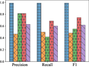
(a) Function - Linux x86

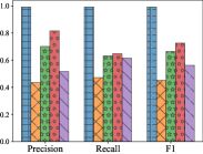
(b) Function - Linux x64

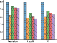
(c) Function - Windows x86

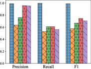
(d) Function - Windows x64

Figure 5: Precision, recall, and F1 score of recovering function boundaries by XDA and other tools on four types of binaries categorized by the platforms and ISAs, on the highest compiler optimization levels.

Generalizability. We test how XDA generalizes to unseen byte sequences. Specifically, we vary the train-test overlap rate and compare the test F1 score achieved by XDA and bi-RNN. We use SPEC CPU2017 binaries compiled on Windows x64 with optimization level Ox as our target for this test. As described in Section VI, we finetune on the model that has been pretrained on SPEC CPU2016 and BAP corpus. We choose 4 target train-test overlap rate (20%, 40%, 60%, and 80%). For each rate, we select as the training set random sequences from the entire testing sequences to construct the target train-test overlap rate.

TABLE III: F1 score (%) of XDA and bi-RNN on recovering function boundaries on varying train-test overlap rate.

	Train-test Overlap Rate
	20%	40%	60%	80%
bi-RNN	70.1	82.3	89.8	96.5
XDA	99.1	99.5	99.8	99.9

Table III shows the testing F1 scores of both XDA and bi-RNN with different train-test overlap rate. Note that in Table II, XDA performs reasonably well on low train-test overlap rate (<3%, see Table I). When we increased the train-test overlap rate, we found that XDA still reaches a 99%+ F1 score after finetuning for 30 epochs. However, bi-RNN obtains a high F1 score only at a high train-test overlap rate (>80%). This supports findings by Andriesse et al. [5] that the performance of previous ML-based tools is biased. One possible explanation is that bi-RNN relies heavily on memorizing syntactic function boundary patterns, and it fails to generalize when the patterns are absent in the training set.

Generalizability to real-world software projects. Besides the dataset in Table I, we also test the strict generalizability of XDA on real-world datasets. In total, we collected 10 real-world popular opensource real-world software projects, including Curl-7.71.1, Diffutils-3.7, GMP-6.2.0, ImageMagick-7.0.10, Libmicrohttpd-0.9.71, LibTomCrypt-1.18.2, OpenSSL-1.0.1f and OpenSSL-1.0.1u, PuTTy-0.74, SQLite-3.34.0, and Zlib-1.2.11. Note that we neither pretrain nor finetune XDA on these software projects, but just use them to test how XDA performs on the unseen binary programs. We thus compile them using GCC-7.5 on Linux x64 with 4 optimizations (O0-O3).

TABLE IV: F1 score of XDA’s function boundary recovery (pretrained on BAP and SPEC CPU2006 and finetuned on SPEC CPU2017 x64 binaries compiled on Linux with GCC) on unseen binaries collected from popular opensource projects.

	O0	O1	O2	O3
Curl	98.6	98.5	98.6	98.2
Diffutils	98.7	98.7	98.8	98.6
GMP	99.2	98.8	98.9	98.6
ImageMagick	98.4	98.3	98.2	98.2
Libmicrohttpd	98.9	98.8	98.9	98.7
LibTomCrypt	99.0	99.0	98.7	98.6
OpenSSL	98.4	98.3	98.4	98.2
PuTTy	98.3	98.3	98.2	98.1
SQLite	98.8	98.7	98.4	98.3
Zlib	98.9	98.9	99.0	98.8

Table IV shows the testing F1 score of each software project and optimization achieved by the model pretrained on BAP and SPEC CPU2006, and finetuned (in 30 epochs) on SPEC CPU2017 x64 binaries compiled on Linux. We find that XDA achieves at least 98.1 (and up to 99.1) F1 score at recovering function boundaries even when none of these binaries are seen during pretraining and finetuning, which is close to the average performance that XDA obtains in Table II.

Tuning false positives/negatives. Some downstream binary analysis tasks, which potentially use XDA as the building block, are highly sensitive to false positives and negatives, depending on their nature. For example, reverse engineering malware can be intolerant of false negatives (e.g., the malicious code is overlooked), while binary re-writer cannot afford false positives (e.g., the data treated as code and getting re-written corrupts the entire program).

While XDA achieves 99%+ F1 score, with only a minimal number of false positives and negatives (Figure 5), we discuss a possible mechanism to tune the false positives/negatives to improve its practicality for diverse downstream tasks. A common practice to control the tradeoff between false positive/negative is to threshold the model’s output probability. For example, we can predict a certain byte as a function boundary only if the model’s output probability on that byte is greater than a threshold. The model can thus be tuned to act more conservatively/aggressively in predicting function boundaries by varying the threshold.

Specifically, we use the ROC (Receiver Operating Characteristics) curve and its AUC (Area Under the Curve) score to quantify the trade-off between false positive/negative. Intuitively, ROC curve measures under different threshold (i.e., beyond what confidence score does the model predict as boundary), what is the model’s resulting false postive rate and false positive rate. The higher the AUC score of the ROC curve, the better the model. Therefore, given such curve, To tune the false positives, we can (ideally) choose the threshold that achieves 0% false positive rate with 100% true positive rate.

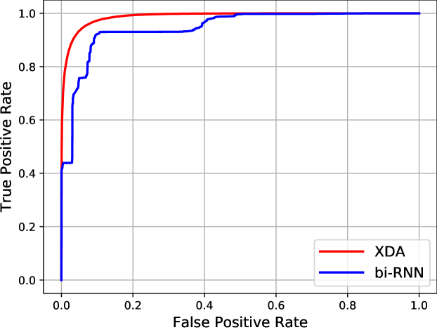
Figure 6: The ROC curve of XDA and bi-RNN, when finetuning and testing on SPEC CPU2017 Windows x64 binaries compiled by MSVC.

Figure 6 shows the ROC curves of XDA and bi-RNN, when they are finetuned for 30 epochs and tested for recovering function boundaries on SPEC CPU2017 Windows x64 binaries compiled on Windows by MSVC. We find that XDA has higher AUC score (0.994) than that of bi-RNN (0.9), which indicates that XDA consistently outperforms bi-RNN on different thresholds.

VII-B RQ2: Robustness

In this section, we analyze the robustness of XDA to high compiler optimization. In Section VII-A, we can see that XDA generalizes well across different platforms, compilers (different platforms imply different compilers), and ISAs, but we have not explicitly shown the robustness on different optimization levels. For example, in Figure 5, we can only see XDA is robust to binaries compiled with the highest optimization. However, we have not seen whether XDA and other disassemblers can remain robust under different optimizations. Therefore, we evaluate the robustness of XDA under varying optimization levels and compare them with bi-RNN.

Robustness to different optimizations. We deliberately chose SPEC CPU2017 x64 binaries compiled on the Windows platform as our target for this test, because these binaries represent the hardest cases in our dataset for an ML model to learn. First, it has less overlapping functions between training and testing than BAP, so simple patterns seen in the training data may not be useful [5]. Second, the function length in SPEC CPU2017 is often very diverse, as opposed to the BAP dataset that has mostly similar-length common library functions. Third, we observe that MSVC uses inline data in the code section for jump tables, while modern versions of GCC keep the code and data separated [4]. Such features make it even harder for recovering function boundaries, as inline data can disrupt the patterns in the code. Finally, the total number of bytes in SPEC CPU2017 is large (see Table I). Since we only keep 10% for training, the large testing set makes it more challenging to obtain good results. Similar to previous setting, the model to be finetuned is pretrained on SPEC CPU2016 and BAP corpus.

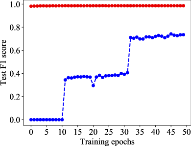
(a) O1

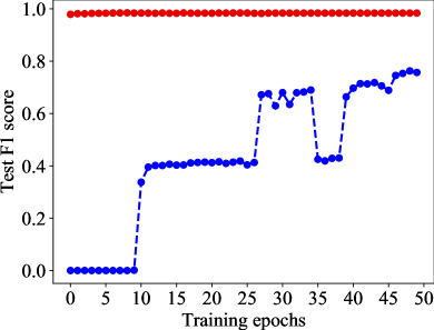
(b) O2

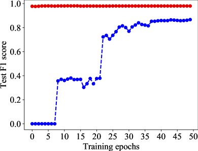
(c) Od

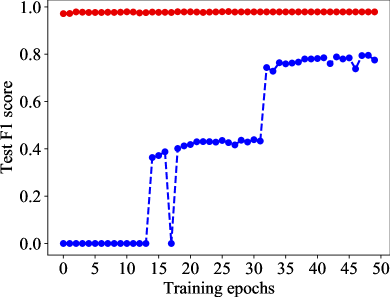
(d) Ox

Figure 7: Comparison between XDA and bi-RNN on recovering function boundaries with varying optimization levels (O1, O2, Ox, Od).

We separate the binaries based on their optimization flags (O1, O2, Od, Ox) and evaluate XDA’s performance of recovering function boundaries. Figure 7 shows the testing F1 scores in 50 training epochs of both XDA and bi-RNN under each optimization level. We find that XDA’s performance remains robust under different optimization levels (>98.8% F1), while bi-RNN performs worse on binaries with higher optimization levels and remains at least 20% worse than XDA on all optimization levels. In addition, impressively, XDA can always reach a very high F1 score even after the first epoch, while bi-RNN struggles in the first 30 epochs.

Transferability across optimization levels. The above experiment tests XDA on different optimization levels, but it still finetunes/trains on all optimization levels. In this experiment, we test if finetuning XDA on only one optimization level can still achieve a good F1 score on another optimization level. We use the same dataset (SPEC CPU2017) and same pretrained model (on SPEC CPU2006 and BAP) described above. We use bi-RNN as the baseline.

Table V shows that XDA always achieves a 98.5%+ F1 score when finetuning on binaries with one optimization level and testing on binaries with another optimization level. However, bi-RNN has an apparent decrease in F1 scores when the training and testing binaries are compiled in different optimization levels. The excellent transferability of XDA implies that the model learns machine code semantics that is robust across different optimization levels.

TABLE V: Test F1 score (%) of XDA and bi-RNN trained and tested on different optimization flags.

		O1	O2	Od	Ox
bi-RNN	O1	81	80	47	2.8
	O2	44	85	81	75
	Od	34.5	4.1	85.2	43.6
	Ox	80	39	44	87
XDA	O1	99.8	98.6	98.8	98.5
	O2	99.8	98.7	99	98.9
	Od	99.6	98.5	99	98.7
	Ox	99.7	98.7	98.8	98.9

Robustness to obfuscated binaries. We also checked how XDA performs on obfuscated binaries, even when we do not pretrain nor finetune XDA on any obfuscated binaries. We obfuscate all our collected real-world software projects (described in Section VII-A) using 5 types of obfuscations (OBF) by Hikari [63] on x64 – an obfuscator based on clang-8. The obfuscation strategies include bogus control flow (bcf), control flow flatening (cff), register-based indirect branching (ibr), basic block splitting (spl), and instruction substitution (sub). We turn off the compiler optimization in case it optimizes away the obfuscated code. We then evaluate the robustness of XDA on each of the software project shown in Table IV obfuscated by each of the obfuscation types.

Table VI lists the F1 score achieved by XDA at recovering function boundaries, with the same pretraining and finetuning setup described in Section VII-A. We observe that XDA remains robust for all obfuscated software projects, achieving at least 98 and up to 99.2 F1 score. Notably, XDA performs the best on the binaries obfuscated by instruction substitution (sub), which is intuitive as such obfuscation only tampers with the arithmetic operation [63] without affecting the function prologues and epilogues Again, we neither pretrained nor finetuned XDA on any obfuscated binaries. Indeed, in practice, we can easily collect a large number of obfuscated binaries for pretraining and finetuning. We thus expect that the model can have even stronger results when it can learn the dependencies between bytes in the obfuscated binaries.

TABLE VI: F1 score of XDA’s function boundary recovery on unseen binaries obfuscated with 5 different obfuscation types.

	bcf	cff	ibr	spl	sub
Curl	98.3	98.5	98.6	98.5	99.0
Diffutils	98.6	98.7	98.4	98.7	99.1
GMP	99.0	98.9	98.9	98.5	99.2
ImageMagick	98.3	98.3	98.1	98.0	98.4
Libmicrohttpd	98.6	98.7	98.8	98.6	98.9
LibTomCrypt	98.7	98.6	98.7	98.6	98.9
OpenSSL	98.3	98.9	98.6	98.9	99.0
PuTTy	98.2	98.1	98.1	98.0	98.3
SQLite	98.7	98.6	98.1	98.4	98.8
Zlib	98.0	98.4	98.1	98.6	99.0

VII-C RQ3: Execution Time

Comparison with other tools. We compare the speed of recovering function boundaries between XDA and two well-known manual-written disassemblers, IDA Pro and Ghidra. Specifically, we choose 4 x64 binaries with different sizes in SPEC CPU2017 compiled by MSVC with O2. We run both IDA and Ghidra in command-line mode to eliminate the runtime overhead of their GUIs. Table VII shows the time taken by each tool to recover the function boundaries from a binary. XDA outperforms both IDA and Ghidra by up to 38$\times$.

GPU vs. CPU. We compare the speed of XDA running on CPUs versus on GPUs. Since XDA’s architecture (i.e., self-attention layers) can be significantly accelerated by GPUs, its inference time on CPU is up to 10$\times$ slower than on a GPU. However, as seen in Table VII, XDA on CPU still typically outperforms IDA and Ghidra by up to 3$\times$.

TABLE VII: Execution time of XDA, IDA, and Ghidra (in seconds) on binaries with different size. We also show the speedup achieved by XDA over the second-fastest tool.

Binary	Size	Speed				XDA speedup
		XDA	XDA	IDA	Ghidra
		GPU	CPU
specrand_is	556K	1.6	12	4.8	16.4	3$\times$
omnetpp_r	4.1M	3.5	29	92.3	146.3	26$\times$
cpuxalan_r	7.8M	4.9	50.1	192.0	185.7	38$\times$
blender_r	22.0M	16.1	136.0	317.1	246.2	15$\times$

VII-D RQ4: Training Efficiency

In this section, we aim to quantify the training efficiency of XDA in comparison with other ML-based tools. Intuitively, since pretraining has already encoded rich knowledge useful for downstream tasks, XDA only requires a small amount of the labeled data and training epochs for finetuning to achieve good results on downstream tasks. In particular, we compare XDA with bi-RNN at recovering function boundaries, on (1) the number of labeled training data required to achieve certain F1 scores, and (2) the number of training epochs needed to achieve specific F1 scores, using the same training data. We use Windows x64 SPEC CPU2017 binaries compiled by MSVC with all 4 optimizations as our dataset. We base the finetuning on the pretrained model on SPEC CPU2006 and BAP.

Labeled training data. We test if XDA requires less training data than bi-RNN to achieve a comparable F1 score. To control the number of labeled training data, we sort the binaries by their size and start with training on the largest binary. Then we gradually increase the number of training binaries (e.g., the second largest, and so on) until the testing F1 score surpasses a chosen threshold. We choose the last half of the sorted binaries as the test set. We choose five F1 score thresholds (0.9, 0.7, 0.5, 0.3, 0.1), and test how many training binaries are required for both XDA and bi-RNN to go beyond these chosen thresholds. We train both models for 30 epochs.

TABLE VIII: The required number of training binaries and epochs by XDA and bi-RNN to surpass the F1 score thresholds.

		F1 score threshold
		$>0.9$	$>0.7$	$>0.5$	$>0.3$	$>0.1$
# training binaries	bi-RNN	N/A	8	4	1	1
	XDA	2	1	1	1	1
# training epochs	bi-RNN	N/A	28	24	14	13
	XDA	2	2	1	1	1

The upper two rows of Table VIII shows that XDA always needs only 1 training binary to surpass 0.7 testing F1 score while 2 binaries to go above 0.9. However, bi-RNN needs at least 8 training binaries to obtain better than 0.7 F1 score. Moreover, it cannot go beyond 0.9, even if it uses up all the remaining 78 training binaries (total 156 binaries except half used for testing).

Training epochs. Now we test if XDA can be trained in less training epochs than bi-RNN to achieve comparable F1 score. Following the above setup, we keep only the largest binary as the training file and take the last half of the sorted binaries as the testing set. We then show the number of required training epochs F1 score in Table VIII (lower two rows) to surpass the same chosen testing threshold defined above. We observe that the number of training epochs required by XDA is much less than bi-RNN. For example, XDA needs at most 2 training epochs to surpass all F1 thresholds, while bi-RNN takes 28 epochs to go beyond 0.7.

VII-E RQ5: Pretraining Effectiveness

Pretraining robustness. We first evaluate the robustness of XDA’s pretraining task, where we test if XDA could transfer the learned knowledge on one platform/compiler/architecture to another for the masked LM task. The rationale is that the compiler idiom varies significantly between platforms and architectures (e.g., calling conventions), generating completely different binaries. Therefore, if the pretrained model on all binaries can generalize to different compiler configurations and instruction sets, we can use a single pretrained model for all downstream tasks instead of pretraining on a specific dataset every time for each finetuning task.

Note that in previous experiments, we pretrained multiple models with different dataset partitions to strictly separate the pretraining and finetuning data (see Section VI) just for the fair comparison with other baselines. However, in practice, we can always collect a large corpus of binaries in the wild for pretraining, and always reuse the same pretrained model for finetuning on different labeled datasets. Pretraining can thus be a one-time cost.

We combine all datasets in Table I, and pretrain 5 different models where their training data is partitioned based on the platforms/compilers or ISAs. Specifically, we pretrain models on (1) all binaries, (2) all Linux x86 binaries, (3) all Linux x64 binaries, (4) all Windows x86 binaries, and (5) all Windows x64 binaries. We leave 4 programs from SPEC CPU2017 dataset out as the test binaries, each from one platform (Windows and Linux) and one ISA (x86 and x64). To test pretrained models on all binaries, we combine all 4 programs as the test set.

TABLE IX: Test PPL of pretrained models. We also include cross-dataset PPL (e.g., train on x86 and test on x64).

	All	Linux x86 GCC/ICC	Linux x64 GCC/ICC	Win x86 MSVC	Win x64 MSVC
All	1.41	1.56	1.25	1.45	1.26
Linux x86 GCC/ICC	2.26	1.55	2.31	2.14	2.88
Linux x64 GCC/ICC	2.41	2.57	1.25	3.03	2.25
Win x86 MSVC	2.26	2.26	2.5	1.44	2.7
Win x64 MSVC	1.98	2.72	2.02	2.5	1.26

Table IX shows the test PPL XDA achieves after 10 epochs of pretraining. When pretrained on all binaries (first row), its PPL drops to at least 1.56. We also test the generalizability of the pretrained model across different platforms and ISAs. We note that XDA also performs reasonably well across binaries. For example, PPL can drop to 2.5 when training on Windows x86 but testing on Linux x64, which is far below that of random guessing (e.g., $2^{-\log(1/256)}=256$). More importantly, pretraining on all binaries (Table IX first row) has obtained the best PPL to all platforms and ISAs (only worse than the cases where training and testing are from the same platforms and ISAs), because its training data includes all type of binaries.

Benefit of pretraining. We quantify how much pretraining can improve the finetuning tasks. Specifically, we test performance of recovering function boundaries on SPEC CPU2017 Windows x64 binaries compiled by MSVC (using 10% random binary as the training set). We compare XDA’s F1 scores achieved by varying pretraining data size. We compare pretrained model on (1) 100% of pretraining data (i.e., on SPEC CPU2006 and BAP), (2) 75% of pretraining data, (3) 50% of pretraining data, (4) 25% of pretraining data, and (5) without pretraining. We also include the F1 scores of bi-RNN for comparison.

Figure 8 shows that pretraining helps greatly in improving the F1 score of recovering function boundaries. The model always reaches >94% F1 score within the first epoch, e.g., even when the model is pretrained on only 25% of pretraining data. With more epochs of finetuning, they can always reach >98% F1 scores. Besides, the more pretraining data, the better the finetuning performance. Without pretraining, XDA’s F1 scores gradually converges to 90% after 28 epochs and are lower than bi-RNN in first 14 epochs. One possible reason is that the underlying model of XDA has many trainable parameters (see Section V-A and Appendix Section -A), which requires more training epochs and data than bi-RNN.

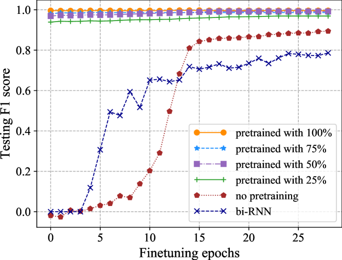
Figure 8: Comparison of testing F1 score on recovering function boundaries between (1) with 100% pretraining data, (2) with 66% pretraining data, (3) with 33% pretraining data, (4) without pretraining, and (5) bi-RNN.

Pretraining other neural architectures. In theory, any neural net architecture can be pretrained, including our bi-RNN baseline. In this paper, we specifically pretrained on the Transformer architecture, as its self-attention layers are known to be amenable to parallelization using GPUs, supporting scalable pretraining. In comparison, recurrent neural network, such as bi-RNN, is known for its limited scalability (due to its sequential nature) on longer sequences and larger datasets [53]. Therefore, given the scale of our pretraining dataset (over 5 gigabytes), training bi-RNN is prohibitively expensive (e.g., our tests show bi-RNN is 100$\times$ slower than the Transformer training on the same amount of data), so we omit pretraining bi-RNN in this paper.

VIII Case Studies

We show some concrete examples to demonstrate that XDA learns various byte dependencies and semantics. We also illustrate the attentions of XDA when making predictions to help explain XDA’s decision process.

VIII-A Probing Learned Semantics

Predicting instructions. Consider the byte sequence shown in Figure 9, taken from the SPEC CPU2017 sgcc compiled by MSVC x64 with O2. We mask out the bytes of whole instruction at 0x3f and feed the sequence to XDA to predict the masked bytes. We find that XDA can recover the correct bytes with high confidence (i.e., >70%). We make following two interesting observations. These observations further justifies the usefulness of pretraining in helping recovering assembly instructions and function boundaries.

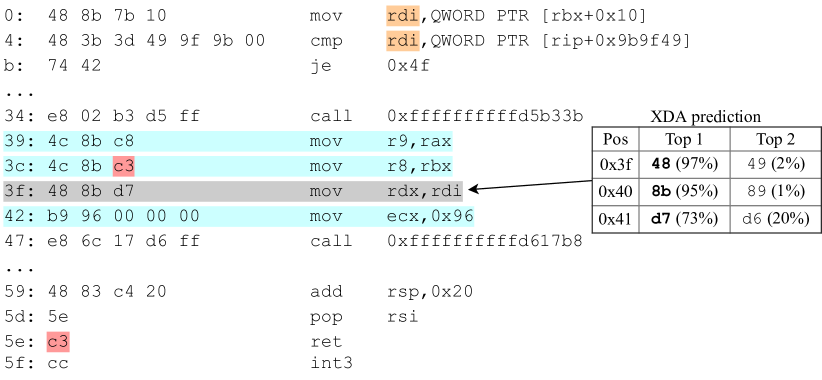
Figure 9: We mask 48 8b d7, one of the argument-passing instructions of the function call at 0x47. XDA’s top-2 predictions with confidence are shown on the right-hand side. We highlight byte c3, as predicting the masked bytes requires distinguishing the meaning of c3, which can be both ret or a register depending on the context. We highlight register rdi where XDA likely leverages to predict rdi in the masked bytes.

XDA learns calling convention. As the masked instruction belong to the argument passing procedures, correctly predicting the exact instructions implies that XDA understands the calling conventions of Windows x64 (i.e., saving arguments to the registers in the order of r9 r8 rdx rcx [45]). We can see that XDA is very confident that the first two bytes are 48 8b (which translates to mov rdx,-), as it has seen the r9 r8 appeared before and ecx (lower 32-bit of rcx). In contrast, it is less certain on the third byte, as moving which register’s value to rdx is harder to infer. Therefore, we see 73% confidence of d7, which will be decoded as rdi, while 20% confidence of d6, which will be decoded as rsi.

XDA learns instruction semantics. Note that the highlighted c3 in the byte sequence have completely different meanings depending on the context. Recall that the input to XDA is only the plain byte sequence. As c3 itself denote ret instruction, If XDA mistakenly treat c3 at location 0x3d as ret, the next most likely bytes would be a sequence of padding bytes cc that usually lie between functions for alignment. Therefore, the only explanation is XDA implicitly learns that c3 at location 0x3d is part of another instruction.

Predicting the gaps between functions. Consider the same binary (SPEC CPU2017 sgcc program compiled by MSVC x64 with O2), where we feed a different byte sequence, as shown in Figure 10, to XDA. We mask out all the padding bytes cc between two functions. The byte before the first cc is a function end at 0x5e, and byte after the last cc is the function start at 0x84.

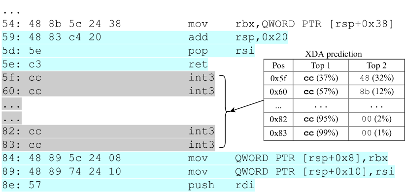
Figure 10: We mask a sequence of padding bytes cc, which reside between two functions. We highlight the typical function prologue/epilogue that XDA leverages to make predictions for the masked bytes.

We can see that XDA predicts all the masked bytes correctly in the right-hand table. As the model cannot leverage any patterns of padding between functions (we have masked out all cc), the only context left for XDA to correctly predict the masked bytes are the function epilogue at 0x5d (pop rsi) to 0x5e (ret), and the following likely function prologue at 0x84 (mov QWORD PTR [rsp+0x8],rbx) to 0x8e (push rdi). As XDA only sees byte sequences, we speculate that XDA must understand that the corresponding bytes before/after the masked bytes represent the function epilogue/prologue, in order to predict those masked bytes are padding. We thus perform a sanity check to ask XDA to predict the function boundary. This time we load the finetuned XDA and feed the same byte sequence without masking and ask the finetuned model to predict the function boundaries. XDA then predicts that there is a function end at 0x5f and a function start at 0x84, which match the ground truth. We thus conclude that the task of predicting masked bytes can effectively help the model to recover function boundaries.

Predicting jump table entries. Consider the vim compiled by Visual Studio x64 with O1 in Figure 11, where we mask out one jump table entry. We can see that XDA correctly predicts all the masked bytes in the jump table with high confidence. More interestingly, we find that while XDA can predict the least significant byte of the jump target (the left-most byte in the jump table entry), it is less confident than predicting other bytes. As the least significant byte is the finest-grained byte the determines the address of the jump target, it is understandable that it is extremely difficult to guess. Moreover, XDA predicts 8b as the second possible candidate byte after 77, as 8b appears twice in the context in other jump table entries. This indicates XDA still leverage the pattern as an important hint, but it is not dominated by only pattern matching because it still predicts 77 as the most probable byte.

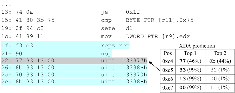
Figure 11: We mask a jump table entry which consists of 4 bytes 77 33 13 00. We highlight the function epilogue and other jump table entries in the context that help XDA to guess the masked bytes.

Predicting local variable allocation size. Consider vim compiled on Windows x64 by Visual Studio with O1 in Figure 12, where we mask out the instruction of decreasing the stack pointer rsp to allocate 40 bytes (0x28) space for local variables. At position 0x24, we can see the corresponding instruction (add rsp, 0x28) that increases the stack pointer to free the space. While the instruction of increasing and decreasing stack pointer are similar with only the third byte (ec and c4, respectively) different, XDA predicts the masked third byte to be ec with 99% confidence. This observation implies that the model is not simply matching similar patterns in its input sequence. Instead, it learns the necessary function prologue/epilogue signature and understands the semantics of underlying instructions, e.g., by correctly predicting local variable size 28 that the program intends to allocate.

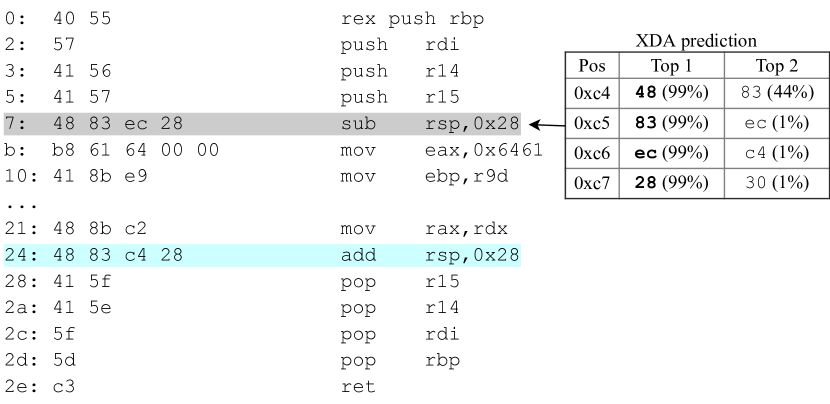
Figure 12: We mask the instruction that adjust the stack pointer to allocate 0x28 (30) bytes on stack for storing the local variable. It consists of 4 bytes 48 83 ec 28. We mark the instruction that increases the stack pointer to free the local variable that XDA leverages to make predictions.

VIII-B Attention Visualization

We visualize XDA’s internal attentions when predicting masked bytes, which explains which input part the model focuses on to make predictions [59, 13]. We use the example of allocating local variables described in Section III to visualize XDA’s attention in predicting the (masked) instruction of local variable allocation. As XDA consists of 12 attention layers with 12 attention heads (detailed in Section V-A), we take the summation from all layers and attention heads.

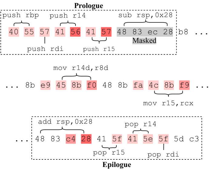
Figure 13: The byte sequence example shown in Figure 3 with more bytes in the context. We illustrate the attention distribution of XDA when predicting the masked bytes (the instruction sub rsp,0x28). The darker the color, the larger the attention value. We put the corresponding instructions beside the most attended bytes.

Figure 13 shows XDA’s attention distribution when predicting the masked bytes 48 83 ec 28. We find that XDA focuses the most on the hints from the prologue and epilogue. For example, it notices (with high attention value) the typical argument passing instructions (push rdi; push r14; push r14; push r15;) before the masked bytes, which strongly indicates the following instruction should be decreasing stack pointer (sub rsp,-) for local variable allocation. Then it focuses on the last two bytes (c4 28) in the instruction add rsp, 0x28, which increases the stack pointer to free the local variable. These two bytes provides the necessary information to decide how many bytes to allocate in the masked instructions. Moreover, it also pays attention to some other instructions (e.g., pop r15; pop r14; pop rdi;) in the epilogue. This probably further validates that the masked instruction resides within a function body, so that it should leverage the bytes c4 28 in the epilogue to predict the masked ec 28. Again, note that all instruction, prologue and epilogue information are provided by us for explanation purpose. XDA does not have access to such information but plain bytes. However, the attention visualization strongly implies that XDA implicitly learns all such knowledge.

IX Related Work

Besides works described in Sections I and II, this section discusses a more comprehensive list of related research papers.

Learned disassembly. Statistical learning has long been used for disassembling and binary analysis [7, 48, 46]. One major path most ML-based approaches take to boost the accuracy is to incorporate the program semantics. For example, Wartell et al. [58] leverage the statistical language modeling to capture byte sequence semantics to compress the binaries. Shingled Graph Disassembly [57] further employs graph-based learning algorithm with cheaper training cost to distinguish code and inline data. Other works [3, 56, 36] introduce control/data-flow to improve the accuracy and robustness. XDA employs masked LM as a pretraining step to automate learning semantics and transfer to downstream disassembly tasks.

Applications based on disassembly. Disassembly serves as the building block for many security-critical applications. For example, binary rewriting and hardening [36, 61] aims to improve the size, efficiency or security of binaries without source code access, and rely on disassembly to recover functions as building blocks for rewriting. Control-flow integrity [37, 1] and code randomization defenses [60] aim to improve the security of binaries by preventing the redirection of control-flow and increasing the difficulty of code injection, respectively. When source code is absent, which is often the case for legacy software in most dire need of such protections, these defenses can be retrofitted to binaries with the help of disassembly and binary rewriting. Decompilation [11, 23] aims to automatically reverse binaries to source code, and relies on disassembly as an initial step to recovering higher-level structure abstracted away during compilation.

Use of ML in other binary analysis tasks. Beyond disassembly, ML has been increasingly applied in other binary analysis tasks. For example, EKLAVYA [12] learns function type signatures. DeepVSA [25] and RENN [38] learn memory alias dependencies. DeepBinDiff [22] and GEMINI [62] learn function similarity by neural embeddings. Most of these methods are based on either recurrent networks or graph neural nets that requires nontrivial engineering effort for encoding domain knowledge, which are shown not as effective as XDA’s underlying self-attention architecture in capturing long-range dependencies, which is also fully-automated [53]. As shown in Section VIII, XDA learns much broader knowledge useful beyond the two tasks considered in this paper. Therefore, we believe XDA has huge potential in other downstream binary analysis tasks and plan to explore in the future work.

X Conclusion

We have presented XDA, a novel disassembling technique based on transfer learning. It leverages machine code semantics learned in pretraining masked Language Modeling to solve downstream disassembly tasks accurately, robustly, and efficiently. XDA is 17.2% more accurate than the state-of-the-art at recovering function boundaries, and achieves a 99.7% F1 score at recovering assembly instructions. Furthermore, XDA is robust against various compilers, architectures, platforms, and optimization levels. Our case studies have shown XDA’s potential for a wide range of downstream disassembly and binary analysis tasks beyond recovering functions and instructions. We open-source XDA at https://github.com/CUMLSec/XDA.

-A XDA Hyperparameters

We describe the hyperparameters that we used throughout all our experiments, if not mentioned elsewhere explicitly.

Network architecture. We use 12 self-attention layers with each having 12 self-attention heads. The embedding dimension is $d_{emb}=768$. We set 3072 as the hidden layer size of MLP $f_{out}$ in the self attention layer. Overall, we have roughly 110 million network parameters. We adopt GeLU [28], known for addressing the problem of vanishing gradient, as the activation function for XDA’s self-attention module. We use the hyperbolic tangent (tanh) as the activation function in finetuning MLP (Equation 2). We set the dropout [52] rate 0.1 for pretraining task while refrain from using dropout in the finetuning task.

Pretraining and finetuning. We fix the largest input length to be 512 and choose the batch size for both pretraining and finetuning as 8. For pretraining we use the update frequency as 16, but for finetuning we set as 4. The update frequency 16 here means the model will aggregate the gradient for 16 batches before it updates the weight parameter. So pretraining has $16\times 8=128$ effective batch size while finetuning has $4\times 8=32$ effective batch size. We choose the smaller update frequency for finetuning is because the training data of finetuning is larger due to the extra labels (unlike pretraining where the data is only input bytes). So we restrict loading too much batch size in case running out of GPU memory. Consequently, to account for the smaller effective batch size, we adopt a relatively smaller learning rate as suggested by the common training tricks [24]. We pick $10^{-5}$ for finetuning while pretraining has a larger learning rate $10^{-4}$ as its effective batch size is larger. Instead of starting with the chosen learning rate at first epoch, we follow the common practice of using small warmup learning rate at first epoch. We use $10^{-7}$ as the initial warmup learning rate, which gets gradually increased until it reaches the actual learning rate after first epoch. Finally, we use use Adam optimizer, with $\beta_{1}=0.9$, $\beta_{2}=0.98$, $\epsilon=10^{-6}$, and weight decay $10^{-2}$.

In this paper, we adopt the hyperparameters that have shown success in other domains such as sentence entailment in natural language processing [17, 31]. For example, we stack 2-layer fully-connected network for finetuning tasks, because finetuning is often assumed as a simple task as the sophisticated dependency learning is offloaded to the pretraining. While it is possible to search for better hyperparameter choices (e.g., more layers or changing connections) from using manual trial [10] to sophisticated algorithms [30], hyperparameter tuning in general is known as an unsolved task. We thus leave the comprehensive studies of tuning XDA’s hyperparameters in our future work.

-B Common Instructions

We include the most common instructions or byte sequences, we include the top 5 n-grams of each dataset in Table X. We choose $n=1,2,3$ as most instruction types can be denoted within these lengths of bytes [29]. We divide each dataset by the instruction set, as x86 and x86-64 can have highly different mapping rules of disassembling instructions. We exclude the most common bytes in the results, such as cc (padding bytes used to call to interrupt procedure), and 00 and ff introduced in two’s complement (for addressing). There are several interesting patterns emerge in the dataset. For example, 8b (MOV instruction) always ranks among the top. When 8b appears in the 2-gram, the top-ranked is 8b 45 in x86, which maps to MOV *, eax. While in x86-64, 48 appears the most, which is the prefix that specifies the 64 bit operand. Therefore, the top 2-gram in x86-64 is 48 8b, which indicates the MOV instruction with 64-bit operand.

TABLE X: Most frequent n-grams (n=1,2,3) for each dataset. We omit the cases that include padding cc, and the common bytes introduced by two’s complement ff and 00.

	x86						x86-64
	1-gram	count	2-gram	count	3-gram	count	1-gram	count	2-gram	count	3-gram	count
SPEC 2017	8b	16,309,260	83 c4	4,055,543	83 c4 10	2,094,343	48	67,406,284	48 8b	23,456,799	20 20 20	3,217,114
	83	11,315,789	44 24	2,747,236	8b 44 24	1,079,364	8b	35,597,922	48 89	14,122,963	48 8b 85	3,105,839
	24	9,407,287	83 ec	2,568,435	83 ec 08	680,529	89	22,438,962	48 8d	7,953,318	48 8b 45	2,417,498
	89	7,644,124	8b 45	2,332,870	89 44 24	633,151	24	17,730,247	44 24	4,730,699	48 89 c7	1,700,933
	e8	7,036,366	c4 10	2,095,990	8b 45 08	592,854	85	14,285,564	48 83	4,475,293	8b 44 24	1,691,308
SPEC 2006	8b	4,411,454	83 c4	1,106,643	83 c4 10	616,278	48	9,048,147	48 8b	3,271,527	48 8b 45	383,183
	83	3,036,396	83 ec	778,944	83 ec 0c	376,601	8b	5,226,813	48 89	2,224,299	8b 44 24	309780
	08	2,112,428	8b 45	656,627	83 ec 08	198,326	89	3,690,654	44 24	868,788	48 89 c7	305,582
	89	2,037,985	c4 10	616,663	8b 45 08	193,443	24	3,152,961	48 83	831,444	89 c7 e8	280,042
	e8	2,014,742	44 24	470,326	8b 44 24	162,405	0f	2,995,076	48 8d	789,078	89 44 24	271,837
BAP	8b	4,859,036	44 24	1,428,109	c7 44 24	554,131	48	7,525,125	48 8b	2,881,802	48 8b 45	534,246
	24	4,753,064	8b 45	1,007,213	89 44 24	474,436	8b	4,495,772	48 89	1,725,358	8b 44 24	233,303
	89	3,503,718	24 04	572,253	44 24 04	385,919	89	3,055,089	48 83	703,937	89 44 24	214,676
	08	2,034,947	c7 44	555,754	89 04 24	326,154	24	2,579,139	44 24	653,945	48 85 c0	185,531
	04	1,919,547	54 24	518,124	8b 44 24	270,141	0f	1,799,445	8b 45	605,920	48 89 c7	180,814

-C Pretraining on all datasets

As described in Section VI, we always keep the data used for pretraining, finetuning, and testing strictly separated, to compare with other baselines fairly. However, as argued in Section VII-E, we can always collect a large corpus of binaries in the wild for pretraining, and always reuse the same pretrained model for finetuning on different labeled datasets. Therefore, we have also pretrained a single model using all datasets available in Table I. We then re-run all finetuning experiments of Table II, and include the updated results in Table XI.

TABLE XI: We update the results of XDA in Table II by using the pretrained model on all available datasets.

Dataset	Platform	ISA	Recovering Function Boundaries F1 (%)					Recovering Instructions F1 (%)
			XDA	Nucleus	bi-RNN	IDA	Ghidra	XDA	bi-RNN	IDA	Ghidra	objdump
SPEC 2017	Linux	x86	98.4	55.4	79.9	91.8	89.0	99.9	87.1	95.9	94.6	100.0†
		x64	99.6	55.0	79.2	90.2	89.5	99.9	88.9	95.8	95.9	100.0†
	Windows	x86	99.9	60.8	73.8	67.6	70.4	99.3	82.3	96.7	92.1	99.3
		x64	99.9	65.0	78.4	78.0	71.6	99.6	81.9	97.1	93.1	99.3
SPEC 2006	Linux	x86	99.8	57.2	86.7	95.7	92.2	99.9	89.0	96.3	95.5	100.0†
		x64	99.9	56.8	73.8	92.8	92.0	99.9	85.9	96.4	94.9	100.0†
	Windows	x86	99.9	68.2	78.5	77.9	76.3	99.9	89.9	98.1	94.5	99.1
		x64	99.9	56.8	72.7	90.1	86.2	99.5	86.2	97.9	95.7	99.4
BAP	Linux	x86	99.6	61.5	74.1	59.0	57.2	N/A∗	N/A∗	N/A∗	N/A∗	N/A∗
		x64	99.7	53.5	79.0	58.3	56.5	N/A∗	N/A∗	N/A∗	N/A∗	N/A∗
	Windows	x86	99.5	69.0	80.1	89.9	87.0	N/A∗	N/A∗	N/A∗	N/A∗	N/A∗
		x64	99.9	70.0	81.4	90.5	80.6	N/A∗	N/A∗	N/A∗	N/A∗	N/A∗
Average			99.6	60.8	78.1	81.8	79.0	99.8	86.4	96.8	94.4	99.6
∗The BAP corpus does not contain source code and PDB files, which are necessary to obtain the assembly instruction ground truth.
†GCC does not generate inline data, so a simple linear disassembler can achieve 100% F1 score [4]. objdump always fails to identify inline data, but because
inline data makes up only a tiny fraction (<1%) of the code section, objdump’s overall F1 score is high.

Table XI shows that the average performance of XDA can be further improved by 0.6% and 0.1% for recovering function boundaries and assembly instructions, respectively. While in such case, pretraining and finetuning data can overlap, note that pretraining does not train with any labels (e.g., function boundaries) but just raw bytes. Indeed, this is the common practice in transfer learning [16, 44, 17, 31].

References

- [1] Martín Abadi, Mihai Budiu, Úlfar Erlingsson, and Jay Ligatti. Control-flow integrity principles, implementations, and applications. ACM Transactions on Information and System Security (TISSEC), 2009.
- [2] National Security Agency. Ghidra Disassembler. https://ghidra-sre.org/.
- [3] Saed Alrabaee, Lingyu Wang, and Mourad Debbabi. BinGold: Towards robust binary analysis by extracting the semantics of binary code as semantic flow graphs (SFGs). Digital Investigation, 2016.
- [4] Dennis Andriesse, Xi Chen, Victor Van Der Veen, Asia Slowinska, and Herbert Bos. An in-depth analysis of disassembly on full-scale x86/x64 binaries. In 25th USENIX Security Symposium, 2016.
- [5] Dennis Andriesse, Asia Slowinska, and Herbert Bos. Compiler-agnostic function detection in binaries. In Proceedings of the 2017 IEEE European Symposium on Security and Privacy, 2017.
- [6] Sanjeev Arora, Hrishikesh Khandeparkar, Mikhail Khodak, Orestis Plevrakis, and Nikunj Saunshi. A theoretical analysis of contrastive unsupervised representation learning. arXiv preprint arXiv:1902.09229, 2019.
- [7] Tiffany Bao, Jonathan Burket, Maverick Woo, Rafael Turner, and David Brumley. BYTEWEIGHT: Learning to Recognize Functions in Binary Code. In 23rd USENIX Security Symposium, 2014.
- [8] Erick Bauman, Zhiqiang Lin, and Kevin W Hamlen. Superset disassembly: Statically rewriting x86 binaries without heuristics. In Proceedings of the 2018 Network and Distributed System Security Symposium (NDSS), 2018.
- [9] Eli Bendersky. PYEFLTOOLS. https://github.com/eliben/pyelftools.
- [10] James Bergstra and Yoshua Bengio. Random search for hyper-parameter optimization. Journal of Machine Learning Research (JMLR), 2012.
- [11] David Brumley, JongHyup Lee, Edward J Schwartz, and Maverick Woo. Native x86 decompilation using semantics-preserving structural analysis and iterative control-flow structuring. In Proceedings of the 22nd USENIX Security Symposium, 2013.
- [12] Zheng Leong Chua, Shiqi Shen, Prateek Saxena, and Zhenkai Liang. Neural nets can learn function type signatures from binaries. In Proceddings of the 26th USENIX Security Symposium, 2017.
- [13] Kevin Clark, Urvashi Khandelwal, Omer Levy, and Christopher D. Manning. What does BERT look at? An analysis of BERT’s attention. In BlackBoxNLP@ACL, 2019.
- [14] Standard Performance Evaluation Corporation. SPEC CPU2006 Benchmark, 2006.
- [15] Standard Performance Evaluation Corporation. SPEC CPU2017 Benchmark, 2017.
- [16] Ido Dagan, Oren Glickman, and Bernardo Magnini. The PASCAL recognising textual entailment challenge. In Machine Learning Challenges Workshop, 2005.
- [17] Jacob Devlin, Ming-Wei Chang, Kenton Lee, and Kristina Toutanova. BERT: Pre-training of deep bidirectional transformers for language understanding. arXiv preprint arXiv:1810.04805, 2018.
- [18] Alessandro Di Federico, Mathias Payer, and Giovanni Agosta. rev.ng: a unified binary analysis framework to recover CFGs and function boundaries. In Proceedings of the 26th International Conference on Compiler Construction, 2017.
- [19] Steven HH Ding, Benjamin CM Fung, and Philippe Charland. Asm2vec: Boosting static representation robustness for binary clone search against code obfuscation and compiler optimization. In 2019 IEEE Symposium on Security and Privacy (S&P), 2019.
- [20] Brendan Dolan-Gavitt, Josh Hodosh, Patrick Hulin, Tim Leek, and Ryan Whelan. Repeatable reverse engineering with PANDA. In Proceedings of the 5th Program Protection and Reverse Engineering Workshop, 2015.
- [21] Yue Duan, Xuezixiang Li, Jinghan Wang, and Heng Yin. DEEPBINDIFF: Learning Program-Wide Code Representations for Binary Diffing. In Network and Distributed System Security Symposium (NDSS), 2020.
- [22] Yue Duan, Xuezixiang Li, Jinghan Wang, and Heng Yin. DEEPBINDIFF: Learning Program-Wide Code Representations for Binary Diffing. In Proceedings of the 2020 Network and Distributed System Security Symposium (NDSS), 2020.
- [23] MV Emmerik and Trent Waddington. Using a decompiler for real-world source recovery. In Proceedings of the 11th Working Conference on Reverse Engineering (WCRE), 2004.
- [24] Priya Goyal, Piotr Dollár, Ross Girshick, Pieter Noordhuis, Lukasz Wesolowski, Aapo Kyrola, Andrew Tulloch, Yangqing Jia, and Kaiming He. Accurate, large minibatch SGD: Training ImageNet in 1 hour. arXiv preprint arXiv:1706.02677, 2017.
- [25] Wenbo Guo, Dongliang Mu, Xinyu Xing, Min Du, and Dawn Song. DEEPVSA: Facilitating Value-set Analysis with Deep Learning for Postmortem Program Analysis. In 28th USENIX Security Symposium (USENIX Security 19), 2019.
- [26] Laune C Harris and Barton P Miller. Practical analysis of stripped binary code. ACM SIGARCH Computer Architecture News, 2005.
- [27] Kaiming He, Xiangyu Zhang, Shaoqing Ren, and Jian Sun. Deep residual learning for image recognition. In Proceedings of the 2016 IEEE conference on computer vision and pattern recognition (CVPR), 2016.
- [28] Dan Hendrycks and Kevin Gimpel. Gaussian error linear units (GELUs). arXiv preprint arXiv:1606.08415, 2016.
- [29] Intel. Intel® 64 and ia-32 architectures software developer’s manual. Volume 3B: System programming Guide, Part, 2011.
- [30] Yann LeCun, Patrice Y Simard, and Barak Pearlmutter. Automatic learning rate maximization by on-line estimation of the hessian’s eigenvectors. In Proceedings of the 1993 Advances in Neural Information Processing Systems (NIPS), 1993.
- [31] Yinhan Liu, Myle Ott, Naman Goyal, Jingfei Du, Mandar Joshi, Danqi Chen, Omer Levy, Mike Lewis, Luke Zettlemoyer, and Veselin Stoyanov. RoBERTa: A robustly optimized BERT pretraining approach. arXiv preprint arXiv:1907.11692, 2019.
- [32] Xiaozhu Meng and Barton P Miller. Binary code is not easy. In Proceedings of the 25th International Symposium on Software Testing and Analysis (ISSTA), 2016.
- [33] Microsoft. Dia2dump. https://docs.microsoft.com/en-us/visualstudio/debugger/debug-interface-access/dia2dump-sample.
- [34] Tomas Mikolov, Kai Chen, Greg Corrado, and Jeffrey Dean. Efficient estimation of word representations in vector space. arXiv preprint arXiv:1301.3781, 2013.
- [35] Tomas Mikolov, Ilya Sutskever, Kai Chen, Greg S Corrado, and Jeff Dean. Distributed representations of words and phrases and their compositionality. In Advances in neural information processing systems, 2013.
- [36] Kenneth Miller, Yonghwi Kwon, Yi Sun, Zhuo Zhang, Xiangyu Zhang, and Zhiqiang Lin. Probabilistic disassembly. In Proceedings of the 41st International Conference on Software Engineering (ICSE), 2019.
- [37] Vishwath Mohan, Per Larsen, Stefan Brunthaler, Kevin W Hamlen, and Michael Franz. Opaque control-flow integrity. In Network and Distributed System Security Symposium (NDSS), 2015.
- [38] Dongliang Mu, Wenbo Guo, Alejandro Cuevas, Yueqi Chen, Jinxuan Gai, Xinyu Xing, Bing Mao, and Chengyu Song. RENN: Efficient Reverse Execution with Neural-network-assisted Alias Analysis. In 2019 34th IEEE/ACM International Conference on Automated Software Engineering (ASE), 2019.
- [39] Myle Ott, Sergey Edunov, Alexei Baevski, Angela Fan, Sam Gross, Nathan Ng, David Grangier, and Michael Auli. fairseq: A Fast, Extensible Toolkit for Sequence Modeling. In Proceedings of NAACL-HLT 2019: Demonstrations, 2019.
- [40] Hui Peng, Yan Shoshitaishvili, and Mathias Payer. T-Fuzz: fuzzing by program transformation. In 2018 IEEE Symposium on Security and Privacy (S&P), 2018.
- [41] Jeffrey Pennington, Richard Socher, and Christopher D Manning. Glove: Global vectors for word representation. In Proceedings of the 2014 conference on empirical methods in natural language processing (EMNLP), 2014.
- [42] Matthew E. Peters, Mark Neumann, Mohit Iyyer, Matt Gardner, Christopher Clark, Kenton Lee, and Luke Zettlemoyer. Deep contextualized word representations. In Proceedings of the 2018 NAACL, 2018.
- [43] Nguyen Anh Quynh. Capstone: Next-gen disassembly framework. Black Hat USA, 2014.
- [44] Pranav Rajpurkar, Jian Zhang, Konstantin Lopyrev, and Percy Liang. Squad: 100,000+ questions for machine comprehension of text. arXiv preprint arXiv:1606.05250, 2016.
- [45] Microsoft. Retrieved. x64 software conventions - stack allocation. https://docs.microsoft.com/en-us/previous-versions/visualstudio/visual-studio-2008/ew5tede7(v=vs.90)?redirectedfrom=MSDN, 2010.
- [46] Nathan E Rosenblum, Xiaojin Zhu, Barton P Miller, and Karen Hunt. Learning to analyze binary computer code. In Proceedings of the 2008 Association for the Advancement of Artificial Intelligence (AAAI), 2008.
- [47] Hex-Rays SA. IDA Pro Disassembler, 2008.
- [48] Eui Chul Richard Shin, Dawn Song, and Reza Moazzezi. Recognizing functions in binaries with neural networks. In 24th USENIX Security Symposium, 2015.
- [49] Yan Shoshitaishvili, Ruoyu Wang, Christophe Hauser, Christopher Kruegel, and Giovanni Vigna. Firmalice-automatic detection of authentication bypass vulnerabilities in binary firmware. In Network and Distributed System Security Symposium (NDSS), 2015.
- [50] Yan Shoshitaishvili, Ruoyu Wang, Christopher Salls, Nick Stephens, Mario Polino, Audrey Dutcher, John Grosen, Siji Feng, Christophe Hauser, Christopher Kruegel, and Giovanni Vigna. SoK: (State of) the art of war: Offensive techniques in binary analysis. In Proceedings of the 2016 IEEE Symposium on Security and Privacy (S&P), 2016.
- [51] Kevin Z Snow, Fabian Monrose, Lucas Davi, Alexandra Dmitrienko, Christopher Liebchen, and Ahmad-Reza Sadeghi. Just-in-time code reuse: On the effectiveness of fine-grained address space layout randomization. In 2013 IEEE Symposium on Security and Privacy, 2013.
- [52] Nitish Srivastava, Geoffrey Hinton, Alex Krizhevsky, Ilya Sutskever, and Ruslan Salakhutdinov. Dropout: A simple way to prevent neural networks from overfitting. The journal of machine learning research (JMLR), 2014.
- [53] Ashish Vaswani, Noam Shazeer, Niki Parmar, Jakob Uszkoreit, Llion Jones, Aidan N Gomez, Łukasz Kaiser, and Illia Polosukhin. Attention is all you need. In Proceedings of the 2017 Advances in Neural Information Processing Systems (NIPS), 2017.
- [54] Giovanni Vigna. Static disassembly and code analysis. In Malware Detection, pages 19–41. Springer, 2007.
- [55] Ruoyu Wang, Yan Shoshitaishvili, Antonio Bianchi, Aravind Machiry, John Grosen, Paul Grosen, Christopher Kruegel, and Giovanni Vigna. Ramblr: Making reassembly great again. In Network and Distributed System Security Symposium (NDSS), 2017.
- [56] Shuai Wang, Pei Wang, and Dinghao Wu. Semantics-aware machine learning for function recognition in binary code. In 2017 IEEE International Conference on Software Maintenance and Evolution (ICSME), 2017.
- [57] Richard Wartell, Yan Zhou, Kevin W Hamlen, and Murat Kantarcioglu. Shingled graph disassembly: Finding the undecidable path. In Proceedings of the Pacific-Asia Conference on Knowledge Discovery and Data Mining (PAKDD), 2014.
- [58] Richard Wartell, Yan Zhou, Kevin W Hamlen, Murat Kantarcioglu, and Bhavani Thuraisingham. Differentiating code from data in x86 binaries. In Joint European Conference on Machine Learning and Knowledge Discovery in Databases, 2011.
- [59] Sarah Wiegreffe and Yuval Pinter. Attention is not not explanation. arXiv preprint arXiv:1908.04626, 2019.
- [60] David Williams-King, Graham Gobieski, Kent Williams-King, James P Blake, Xinhao Yuan, Patrick Colp, Michelle Zheng, Vasileios P Kemerlis, Junfeng Yang, and William Aiello. Shuffler: Fast and deployable continuous code re-randomization. In Proceedings of the 12th USENIX Symposium on Operating Systems Design and Implementation (OSDI), 2016.
- [61] David Williams-King, Hidenori Kobayashi, Kent Williams-King, Graham Patterson, Frank Spano, Yu Jian Wu, Junfeng Yang, and Vasileios P. Kemerlis. Egalito: Layout-agnostic binary recompilation. In Proceedings of the 25th International Conference on Architectural Support for Programming Languages and Operating Systems (ASPLOS), 2020.
- [62] Xiaojun Xu, Chang Liu, Qian Feng, Heng Yin, Le Song, and Dawn Song. Neural network-based graph embedding for cross-platform binary code similarity detection. In Proceedings of the 2017 ACM SIGSAC Conference on Computer and Communications Security, 2017.
- [63] Naville Zhang. Hikari – an improvement over Obfuscator-LLVM. https://github.com/HikariObfuscator/Hikari, 2017.