Enriching Word Embeddings with Temporal and Spatial Information

Abstract

The meaning of a word is closely linked to sociocultural factors that can change over time and location, resulting in corresponding meaning changes. Taking a global view of words and their meanings in a widely used language, such as English, may require us to capture more refined semantics for use in time-specific or location-aware situations, such as the study of cultural trends or language use. However, popular vector representations for words do not adequately include temporal or spatial information. In this work, we present a model for learning word representation conditioned on time and location. In addition to capturing meaning changes over time and location, we require that the resulting word embeddings retain salient semantic and geometric properties. We train our model on time- and location-stamped corpora, and show using both quantitative and qualitative evaluations that it can capture semantics across time and locations. We note that our model compares favorably with the state-of-the-art for time-specific embedding, and serves as a new benchmark for location-specific embeddings.

1 Introduction

The use of word embeddings as a form of lexical representation has transformed the use of natural language processing for many applications such as machine translation Qi et al. (2018) and language understanding Peters et al. (2018). The changing of word meaning over the course of time and space, termed semantic drift, has been the subject of long standing research in diachronic linguistics Ullmann (1979); Blank (1999). Additionally, the emergence of distinct geographically-qualified English varieties (e.g., South African English) has given rise to salient lexical variation giving several English words different meanings depending on the geographic location of their use, as documented in studies on World Englishes Kachru et al. (2006); Mesthrie and Bhatt (2008). Considering the multiplicity of meanings that a word can take over the span of time and space owing to inevitable linguistic, and sociocultural factors among others, a static representation of a word as a single word embedding seems rather limited. Take the word apple as an example. Its early to near-recent mentions in written documents referred only to a fruit, but in the recent times it is also the name of a large technology company. Another example is the title for the head of government, which is “president” in the USA, and is “prime minister” in Canada.

Naturally, we expect that one word should have different representations conditioned on the time or location. In this paper, we study how word embeddings can be enriched to encode their semantic drift in time and space. Extending a recent line of research on time-specific embeddings, including the works by Bamler and Mandt and Yao et al., we propose a model to capture varying lexical semantics across different conditions—of time and location.

A key technical challenge of learning conditioned embeddings is to put the embeddings (derived from different time periods or geographical locations) in the same vector space and preserve their geometry within and across different instances of the conditions.Traditional approaches involve a two-step mechanism of first learning the sets of embeddings separately under the different conditions, and then aligning them via appropriate transformations Kulkarni et al. (2015); Hamilton et al. (2016); Zhang et al. (2016). A primary limitation of these methods is their inadequate representation of word semantics, as we show in our comparative evaluation. Another approach to conditioned embedding uses a loss function with regularizers over word embeddings across conditions for their smooth trajectory in the vector space Yao et al. (2018). However, its scope is limited to modeling semantic drift over only time.

We propose a model for general conditioned embeddings, with the novelty that it explicitly preserves embedding geometry under different conditions and captures different degrees of word semantic changes. We summarize our contributions below.

1. We propose an unsupervised model to learn condition-specific embeddings including time-specific and location-specific embeddings;

2. Using benchmark datasets we demonstrate the state-of-the-art performance of the proposed model in accurately capturing word semantics across time periods and geographical regions;

3. We provide the first dataset to evaluate word embeddings across locations to foster research in this direction.

2 Related Works

Time-specific embeddings. The evolution of word meaning with time has been widely studied in sociolinguistics Ullmann (1979); Tang (2018). Early approaches to uncovering these trends have relied on frequency based models which use frequency changes to trace semantic shift over time Lijffijt et al. (2012); Choi and Varian (2012); Michel et al. (2011). More recent works have sought to study these phenomena using distributional models Kutuzov et al. (2018); Huang and Paul (2019); Schlechtweg et al. (2020).

Existing approaches on time-specific embeddings can be divided into three categories: aligning independently trained embeddings across time, joint training of time-dependent embeddings and using contextualized vectors from pre-trained models. The first type of approaches include the work by Kulkarni et al., and that of Hamilton et al. and Zhang et al.. They pre-trained multiple sets of embeddings for different times independently, and aligned one set of embedding with another set so that two sets of embeddings were comparable.

The second approach—joint training—aims to guarantee the alignment of embeddings in the same vectors space so that they are directly comparable. Compared with the previous category of approaches, the joint learning of time-stamped embeddings has shown improved abilities to capture semantic changes across time. Bamler and Mandt used a probabilistic model to learn time-specific embeddings Bamler and Mandt (2017). They put Gaussian assumption on the evolution of embeddings to guarantee the embedding alignment. Yao et al. learned embeddings by the factorization of positive pointwise mutual information (PPMI) matrix. They imposed L2 constraints on embeddings from neighboring time periods for embedding alignment Yao et al. (2018). Rosenfeld and Erk proposed a neural model to first encode time and word information respectively and then to learn time-specific embeddings Rosenfeld and Erk (2018). Dubossarsky et al. aligned word embeddings by sharing their context embeddings at different times Dubossarsky et al. (2019).

Some recent works fall in the third category, retrieving contextualized representations from pre-trained models such as BERT Devlin et al. (2018) as time-specific sense embeddings of words Hu et al. (2019); Giulianelli et al. (2020). These pre-trained embeddings are limited to the scope of local contexts, while we learn the global representation of words in a given time or location.

The underlying mathematical models of these previous works on temporal embeddings are discussed in the supplementary material. Our model belongs to the second category of joint embedding training. Different from previous works, our embedding is based on a model which explicitly takes into account the important semantic properties of time-specific embeddings.

Embedding with spatial information. Lexical semantics is also sensitive to spatial factors. For example, the word denoting the regional head may be used differently depending on the region. For instance, the word may refer to president, or prime minister or king depending on the region. Language variation across regional contexts has been analyzed in sociolinguistics and dialectology studies (e.g.,Silva-Corvalán (2006); Kulkarni et al. (2016)). It is also understood that a deeper understanding of semantics enhanced with location information is critical to location-sensitive applications such as content localization of global search engines Brandon Jr (2001).

Some approaches towards this include, a latent variable model proposed for geographical linguistic variation Eisenstein et al. (2010) and a skip-gram model for geographically situated language Bamman et al. (2014). The current study is most similar to Bamman et al. (2014) with the overlap in our intents to learn location-specific embeddings for measuring semantic drift. Most studies on location-dependent language resort to a qualitative evaluation, whereas Bamman et al. (2014) resorts to a quantitative analysis for entity similarity. However, it is limited to a given region without exploring semantic equivalence of words across different geographic regions. To the extent we are aware, this is the first study to present a quantitative evaluation of word representations across geographical regions with the use of a dataset.

3 Model

We now introduce the model on which the condition-specific embedding training is based in this section. We assume access to a corpus divided into sub-corpora based on their conditions (time or location), and texts in the same condition (e.g., same time period) are gathered in each sub-corpus. For each condition, the co-occurrence counts of word pairs gathered from its sub-corpus are the corpus statistics we use for the embedding training. We note that because these sub-corpora vary in size, we scale the word co-occurrences of every condition so that all sub-corpora have the same total number of word pairs. We term the scaled value of word co-occurrences of word $w_{i}$ and $w_{j}$ in condition $c$ as $\mathbf{X}_{i,j,c}$.

A static model (without regard to the temporal or spatial conditions) proposed by Arora et al. provides the unifying theme for the seemingly different embedding approaches of word2vec and GloVe. In particular, It reveals that corpus statistics such as word co-occurrences could be estimated from embeddings. Inspired by this, we proposed a model for conditioned embeddings, and characterize such a model by its ability to capture the lexical semantic properties across different conditions.

3.1 Properties of Conditioned Embeddings

Before exploring the details of our model for condition-specific embeddings, we discuss some desired semantic properties of these embeddings. We expect the embeddings to capture time- and location-sensitive lexical semantics. We denote by $c$ the condition we use to refine word embeddings, which can be a specific time period or a location. We then have temporal embeddings if the condition is time period, and spatial embeddings if the condition is location. For a word $w$, the condition-specific word embedding for condition $c$ is denoted as $\mathbf{v}_{w,c}$. The key semantic properties of the condition-specific word embedding, which we consider in our model are:
(1) Preservation of geometry. One geometric property of static embeddings is that the difference vector encodes word relations, i.e., $\mathbf{v}_{\text{bigger}}-\mathbf{v}_{\text{big}}\approx\mathbf{v}_{\text{greater}}-\mathbf{v}_{\text{great}}$ Mikolov et al. (2013). Analogously, for the condition-specific embedding of semantically stable words across conditions, given word pairs $(w_{1},w_{2})$ and $(w_{3},w_{4})$ with the same underlying lexical relation, we expect the following equation to hold in any condition $c$.

$$\mathbf{v}_{w_{1},c}-\mathbf{v}_{w_{2},c}\approx\mathbf{v}_{w_{3},c}-\mathbf{v}_{w_{4},c}.$$ (1)

This property is implicitly preserved in approaches aligning independently trained embeddings with linear transformations Kulkarni et al. (2015).
(2) Consistency over conditions. Most word meanings change slowly over a given condition, i.e., their condition-specific word embeddings should be highly correlated Hamilton et al. (2016). When the condition is time period, for example, $c_{1}$ is the year 2000, and $c_{2}$ is the year 2001, we expect that for a given word, $\mathbf{v}_{w,c_{1}}$ and $\mathbf{v}_{w,c_{2}}$ have high similarity given their temporal proximity. The consistency property is preserved in models which jointly train embeddings across conditions (e.g., Yao et al. (2018)).
(3) Different degrees of word change. Although word meanings change over time, not all words undergo this change to the same degree; some words change dramatically while others stay relatively stable across conditions Blank (1999). In our formulation, we require the representation to capture the different degrees of word meaning change. This property is unexplored in prior studies.

We incorporate these semantic properties as explicit constraints into our model for condition-specific embeddings, which we formulate as an optimization problem.

3.2 Model

We propose a model that generates embeddings satisfying the semantic properties as discussed above. Writing the embedding $\mathbf{v}_{w,c}$ of word $w$ in condition $c$ as a function of its condition-independent representation $\mathbf{v}_{w}$, condition representation vector $\mathbf{q}_{c}$ and deviation embedding $\mathbf{d}_{w,c}$:

$$\mathbf{v}_{w,c}=\mathbf{v}_{w}\odot\mathbf{q}_{c}+\mathbf{d}_{w,c},$$ (2)

where $\odot$ is Hadamard product (i.e., elementwise multiplication). We decompose the conditioned representation into three component embeddings. This novel representation is motivated by the intuition that a word $w$ usually carries its basic meaning $\mathbf{v}_{w}$ and its meaning is influenced by different conditions represented by $\mathbf{q}_{c}$. Moreover, words have different degrees of meaning variation, which is captured by the deviation embedding $\mathbf{d}_{w,c}$.

We begin with a model proposed by Arora et al. for static word embeddings regardless of the temporal or spatial conditions Arora et al. (2016). Let $\mathbf{v}_{w}$ be the static representation of word $w$. For a pair of words $w_{1}$ and $w_{2}$, the static model assumes that

$$\log\mathbb{P}(w_{1},w_{2})\approx\frac{1}{2}\lVert\mathbf{v}_{w_{1}}+\mathbf{v}_{w_{2}}\rVert^{2},$$ (3)

where $\mathbb{P}(w_{1},w_{2})$ is the co-occurrence probability of these two words in the training corpus.

Let $\mathbb{P}_{c}(w_{1},w_{2})$ be the co-occurrence probability of word pair $(w_{1},w_{2})$ in the condition $c$. Based on the static model in Eq. (3), for a condition $c$ we have

$$\log\mathbb{P}_{c}(w_{1},w_{2})\approx\frac{1}{2}\lVert\mathbf{v}_{w_{1},c}+\mathbf{u}_{w_{2},c}\rVert^{2}.$$ (4)

Here, borrowing ideas from previous embedding algorithms including word2vec Mikolov et al. (2013) and GloVe Pennington et al. (2014), we use two sets of word embeddings $\{\mathbf{v}_{w,c}\}$ and $\{\mathbf{u}_{w,c}\}$ for a word $w_{1}$ and its context word $w_{2}$ respectively in condition $c$. Accordingly, we have two sets of condition-independent embeddings $\{\mathbf{v}_{w}\}$ and $\{\mathbf{u}_{w}\}$, and two sets of deviation vectors $\{\mathbf{d}_{w_{,}c}\}$ and $\{\mathbf{d}^{\prime}_{w,c}\}$. The condition-specific embeddings in Eq. (2) can be written as:

$$\left\{\begin{array}[]{cc}\mathbf{v}_{w_{1},c}&=\mathbf{v}_{w_{1}}\odot\mathbf{q}_{c}+\mathbf{d}_{w_{1},c}\\ \mathbf{u}_{w_{2},c}&=\mathbf{u}_{w_{2}}\odot\mathbf{q}_{c}+\mathbf{d}^{\prime}_{w_{2},c}\end{array}\right.$$ (7)

By combining Eq. (4) and (7), we derive the model for condition-specific embeddings:

$$\log\mathbb{P}_{c}(w_{1},w_{2}) \approx\frac{1}{2}\lVert\mathbf{(}\mathbf{v}_{w_{1}}\odot\mathbf{q}_{c}+\mathbf{d}_{w_{1},c})$$

$$+(\mathbf{u}_{w_{2}}\odot\mathbf{q}_{c}+\mathbf{d}_{w_{2},c}^{\prime})\rVert^{2}.$$ (8)

This model can be simplified as

$$\log\mathbb{P}_{c}(w_{1},w_{2})\approx b_{w_{1},c}+b_{w_{2},c}^{\prime}+$$

$$(\mathbf{v}_{w_{1}}\odot\mathbf{q}_{c}+\mathbf{d}_{w_{1},c})^{T}(\mathbf{u}_{w_{2}}\odot\mathbf{q}_{c}+\mathbf{d}_{w_{2},c}^{\prime}),$$ (9)

where $b_{w_{1},c}$ and $b_{w_{2},c}^{\prime}$ are bias terms introduced to replace the terms $\lVert\mathbf{v}_{w_{1},c}\rVert^{2}$ and $\lVert\mathbf{u}_{w_{2},c}\rVert^{2}$ respectively. We document the derivation details of Eq. (9) in the supplementary material.

Optimization problem. This model enables us to use the conditioned embeddings to estimate the word co-occurrence probabilities in a specific condition. Conversely, we can formulate an optimization problem to train the conditioned embeddings from the word co-occurrences based on our model.

We count the co-occurrences of all word pairs ($w_{1}$, $w_{2}$) in different conditions based on the respective sub-corpora. For example, we count word co-occurrences over different time periods to incorporate temporal information into word embeddings, and we count word pairs in different locations to learn spatially sensitive word representations.

Recall that $\mathbf{X}_{i,j,c}$ is the scaled co-occurrence counts of $w_{i}$ and $w_{j}$ in condition $c$. Denote by $W$ the total vocabulary and by $C$ the number of conditions, where $C$ is the number of time bins for the temporal condition or the number of locations for the location condition. Suppose that $\mathbf{V}$ is an $(m\times|W|)$ condition-independent word embedding matrix, where each column corresponds to an $m$-dimension word vector $\mathbf{v}_{w}$. Matrix $\mathbf{U}$ is an $(m\times|W|)$ basic context embedding matrix with each column as a context word vector $\mathbf{u}_{w}$. Matrix $\mathbf{Q}$ is an $(m\times C)$ matrix, where each column is a condition vector $\mathbf{q}_{c}$. As for deviation matrices, $\mathbf{D}_{m\times|W|\times C}$ and $\mathbf{D}^{\prime}_{m\times|W|\times C}$ consist of $m$-dimension deviation vectors $\mathbf{d}_{w,c}$ and $\mathbf{d}_{w,c}^{\prime}$ respectively for word $w$ in condition $c$.

Our goal is to learn embeddings $\mathbf{U}$, $\mathbf{Q}$ and $\mathbf{D}$ so as to approximate the word co-occurrence counts based on the model in Eq.(9). Here, we design a loss function to be the approximation error of the embeddings, which is the mean square error between the condition-specific co-occurrences counted from the respective sub-corpora and their estimates from the embeddings.

To satisfy the property 2 of condition-specific embeddings, we impose $L_{2}$ constraints $\lVert\mathbf{q}_{a}-\mathbf{q}_{b}\rVert^{2}$ on the embeddings of condition $a$ and $b$ to guarantee the consistency over conditions. For time-specific embeddings, the constraints are for adjacent time bins. As for location-sensitive embeddings, the constraints are for all pairs of location embeddings.

Furthermore, to account for the slow change in meaning of most words across conditions (as in time periods or locations) listed as property 3 of conditioned embeddings, we also include $L_{2}$ constraints $\lVert\mathbf{D}\rVert^{2}$ and $\lVert\mathbf{D}^{\prime}\rVert^{2}$ on the deviation terms to penalize big changes.

Putting together the approximation error, constraints on condition embeddings and deviations, we have the following loss function:

$$L= \sum\limits_{c=1}^{C}\sum\limits_{i=1}^{|W|}\sum\limits_{j=1}^{|W|}\left((\mathbf{V}_{i}\odot\mathbf{Q}_{c}+\mathbf{D}_{i,c})^{T}(\mathbf{U}_{j}\odot\mathbf{Q}_{c}+\mathbf{D}_{j,c}^{\prime})\right.$$

$$\left.+\mathbf{b}_{i,c}+\mathbf{b}_{j,c}^{\prime}-\log(\mathbf{X}_{i,j,c})\right)^{2}$$

$$+\frac{\alpha}{2}\sum\limits_{a,b}\lVert\mathbf{Q}_{a}-\mathbf{Q}_{b}\rVert^{2}+\frac{\beta}{2}(\lVert\mathbf{D}\rVert^{2}+\lVert\mathbf{D}^{\prime}\rVert^{2}).$$ (10)

In addition to ensuring a smooth trajectory of the embeddings, the penalization on the deviations $\mathbf{D}$ and $\mathbf{D}^{\prime}$ is necessary to avoid the degenerate case that $\mathbf{Q}_{c}=\bf{0},\forall c$.

We note that, for the constraint on condition embeddings in the loss function $L$, for time-specific embeddings we use $\sum\limits_{c=1}^{C-1}\lVert\mathbf{Q}_{c+1}-\mathbf{Q}_{c}\rVert^{2}$, whereas for location-specific embeddings, the constraint becomes $\sum\limits_{a=1}^{C-1}\sum\limits_{b=a+1}^{C}\lVert\mathbf{Q}_{a}-\mathbf{Q}_{b}\rVert^{2}$.

Model Properties. We have presented our approach to learning conditioned embeddings. Now we will show that the proposed model satisfies the aforementioned key properties in Section 3.1. We start with the property of geometry preservation. For a set of semantically stable words $S=\{w_{1},w_{2},w_{3},w_{4}\}$, it is known that $d_{w,c}\approx 0$ for $w\in S$. Suppose that the relation between $w_{1}$ and $w_{2}$ is the same as the relation between $w_{3}$ and $w_{4}$, i.e., $\mathbf{v}_{w_{1}}-\mathbf{v}_{w_{2}}=\mathbf{v}_{w_{3}}-\mathbf{v}_{w_{4}}.$ Given Eq. (2) for any condition $c$, it holds that

$$\mathbf{v}_{w_{1},c}-\mathbf{v}_{w_{2},c}\approx(\mathbf{v}_{w_{1}}-\mathbf{v}_{w_{2}})\odot q_{c}$$

$$\approx(\mathbf{v}_{w_{3}}-\mathbf{v}_{w_{4}})\odot q_{c}\approx\mathbf{v}_{w_{3},c}-\mathbf{v}_{w_{4},c}.$$ (11)

As for the second property of consistency over conditions, we again consider a stable word $w$. Its conditioned embedding $v_{w,c}$ in condition $c$ can be written as $\mathbf{v}_{w,c}=\mathbf{v}_{w}\odot\mathbf{q}_{c}$. As is shown in Eq. (10), the $L_{2}$ constraint $\lVert\mathbf{q}_{a}-\mathbf{q}_{b}\rVert^{2}$ is put on different condition embeddings. The difference between word embeddings of $w$ under two conditions $a$ and $b$ are:

$$\lVert\mathbf{v}_{w,a}-\mathbf{v}_{w,b}\rVert^{2} =\lVert\mathbf{v}_{w}\odot(\mathbf{q}_{a}-\mathbf{q}_{b})\rVert^{2}$$

$$\leq\frac{1}{2}\lVert\mathbf{v}_{w}\rVert^{2}\cdot\lVert\mathbf{q}_{a}-\mathbf{q}_{b}\rVert^{2}.$$ (12)

According to Cauchy-Schwartz inequality, the $L_{2}$ constraint on condition vectors $\mathbf{q}_{a}-\mathbf{q}_{b}$ also acts as a constraint on word embeddings. With a large coefficient $\alpha$, it prevents the embedding from differing too much across conditions, and guarantees the smooth trajectory of words.

Lastly we show that our model captures the degree of word changes. The deviation vector $\mathbf{d}_{w,c}$ we introduce in the model captures such changes. The $L_{2}$ constraint on $\lVert\mathbf{d}_{w,c}\rVert$ shown in Eq. (10) forces small deviation on most words which are smoothly changing across conditions. We assign a small coefficient $\beta$ to this constraint to allow sudden meaning changes in some words. The hyperparameter setting is discussed below.

Embedding training. We have hyperparameters $\alpha$ and $\beta$ as weights on the word consistency and the deviation constraints. We set $\alpha=1.5$ and $\beta=0.2$ in time-specific embeddings, and $\alpha=1.0$ and $\beta=0.2$ in location-specific embeddings.

At each training step, we randomly select a nonzero element $x_{i,j,c}$ from the co-occurrence tensor $\mathbf{X}$. Stochastic gradient descent with adaptive learning rate is applied to update $\mathbf{V}$, $\mathbf{U}$, $\mathbf{Q}$, $\mathbf{D}$, $\mathbf{D}^{\prime}$, $\mathbf{d}$ and $\mathbf{d}^{\prime}$, which are relevant to $x_{i,j,c}$ to minimize the loss $L$. The complexity of each step is $O(m)$, where $m$ is the embedding dimension. In each epoch, we traverse all nonzero elements of $\mathbf{X}$. Thus we have $\text{nnz}(\mathbf{X})$ steps where $\text{nnz}(\cdot)$ is the number of nonzero elements. Although $\mathbf{X}$ contains $O(|W|^{2})$ elements, $\mathbf{X}$ is very sparse since many words do not co-occur, so $\text{nnz}(\mathbf{X})\ll|W|^{2}$. The time complexity of our model is $O(E\cdot m\cdot\text{nnz}(\mathbf{X}))$ for $E-$epoch training. We set $E=40$ in training both temporal and spatial word embeddings.

Postprocessing. We note that embeddings under the same condition are not centered, i.e., the word vectors are distributed around some non-zero point. We center these vectors by removing the mean vector of all embeddings in the same condition. The centered embedding $\tilde{\mathbf{v}}_{w,c}$ of word $w$ under condition $c$ is:

$$\tilde{\mathbf{v}}_{w,c}=\mathbf{v}_{w,c}-\frac{1}{|W|}\sum\limits_{\bar{w}\in W}\mathbf{v}_{\bar{w},c}.$$ (13)

The similarity between words across conditions is measured by the cosine similarity of their centered embeddings $\{\tilde{\mathbf{v}}_{w,c}\}$.

Across time	the, in, to, a, of, it, by, with, at, was, are, and, on, who, for, not, they, but, he, is, from, have, as, has, their, about, her, been, there, or, will, this, said, would
Across regions	in, from, at, could, its, which, out, but, on, all, has, so, is, are, had, he, been, by, an, it, as, for, was, this, his, be, they, we, her, that, and, with, a, of, the

Table 1: Stable Words across Time and Locations

4 Experiments

In this section, we compare our condition-specific word embedding models with corresponding state-of-the-art models combined with temporal or spatial information. The dimension of all vectors is set as $50$. We have the following baselines:
(1) Basic word2vec (BW2V). It is word2vec CBOW model, which is trained on the entire corpus without considering any temporal or spatial partition Mikolov et al. (2013);
(2) Transformed word2vec (TW2V). Multiple sets of embeddings are trained separately for each condition. Two sets of embeddings are then aligned via a linear transformation Kulkarni et al. (2015).
(3) Aligned word2vec (AW2V): Similar to TW2V, sets of embeddings are first trained independently and then aligned via orthonormal transformations Hamilton et al. (2016).
(4) Dynamic word embedding (DW2V): This approach proposes a joint training of word embeddings at different times with alignment constraints on temporally adjacent sets of embeddings Yao et al. (2018). We modify this baseline for location based embeddings by putting its alignment constraints on every two sets of embeddings.

4.1 Training Data

We used two corpora as training data–the time-stamped news corpus of the New York Times collected by Yao et al. (2018) to train time-specific embeddings and a collection of location-specific texts in English, provided by the International Corpus of English project ICE (2019) for location-specific embeddings.

New York Times corpus. The news dataset from New York Times consists of $99,872$ articles from 1990 to 2016. We use time bins of size one-year, and divide the corpus into 27 time bins.

International Corpus of English (ICE). The ICE project collected written and spoken material in English (one million words each) from different regions of the world after 1989. We used the written portions collected from Canada, East Africa, Hong Kong, India, Ireland, Jamaica, the Philippines, Singapore and the United States of America.

Deviating from previous works, which remove both stop words and infrequent words from the vocabulary Yao et al. (2018), we only remove words with observed frequency count less than a threshold. We keep the stop words to show that the trained embedding is able to identify them as being semantically stable. The frequency threshold is set to $200$ (the same as Yao et al. (2018)) for the New York Times corpus, and to $5$ for the ICE corpus given that the smaller size of ICE corpus results in lower word frequency than the news corpus.

We evaluate the enriched word embeddings for the following aspects:

1. Degree of semantic change. As mentioned in the list of desired properties of conditioned embeddings, words undergo semantic change to different degrees. We check whether our embeddings can identify words whose meanings are relatively stable across conditions. These stable words will be discussed as part of the qualitative evaluation.

2. Discovery of semantic change. Besides stable words, we also study words whose meaning changes drastically over conditions. Since a word’s neighbors in the embedding space can reflect its meaning, we find the neighbors in different conditions to demonstrate how the word meaning changes. The discovery of semantic changes will be discussed as part of our qualitative evaluation.

3. Semantic equivalence across conditions. All condition-specific embeddings are expected to be in the same vector space, i.e., the cosine similarity between a pair of embeddings reflects their lexical similarity even though they are from different condition values. Finding semantic equivalents with the derived embeddings will be discussed in the quantitative evaluation.

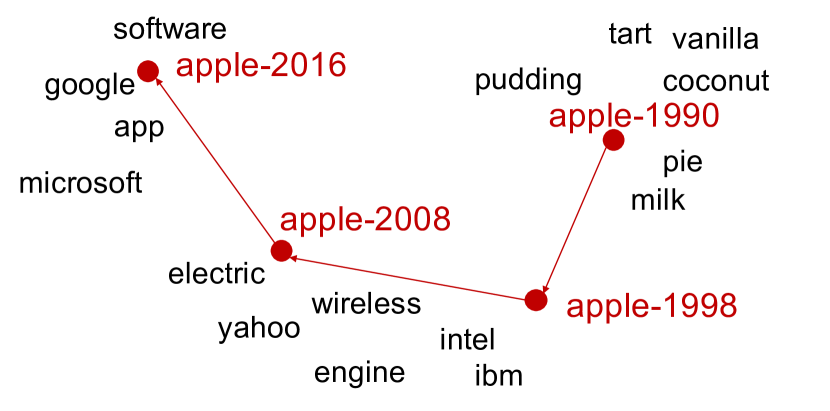
(a) Word “apple” and its neighbors across time.

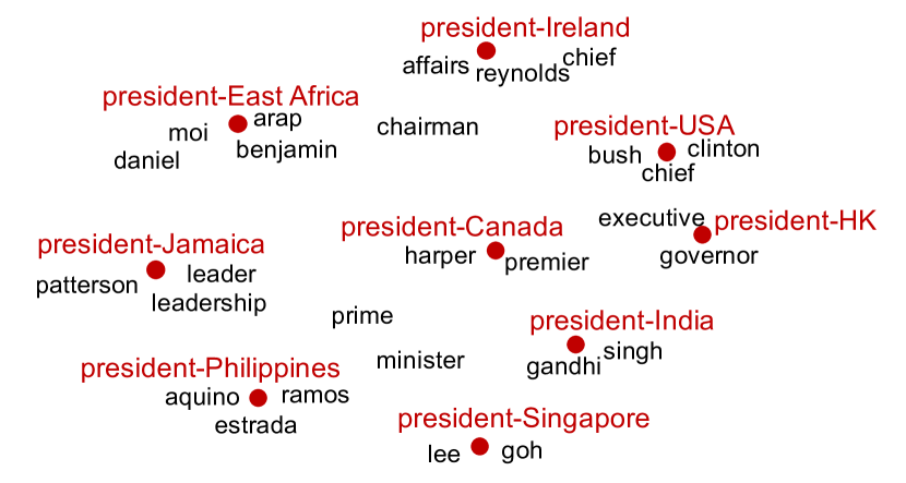
(b) Word “president” and its neighbors across locations.

Figure 1: The trajectory of word embeddings over time and locations.

4.2 Qualitative Evaluation

We first identify words that are semantically stable across time and locations respectively. Cosine similarity of embeddings reflects the semantic similarity of words. The embeddings of stable words should have high similarity across conditions since their semantics do not change much with conditions. Therefore, we average the cosine similarity of words between different time durations or locations as the measure of word stability, and rank the words in terms of their stability. The most stable words are listed in Table 1. We notice that a vast majority of these stable words are frequent words such as function words. It may be interpreted based on the fact that these are words that encode structure Gong et al. (2017, 2018), and that the structure of well-edited English text has not changed much across time or locations Poirier (2014). It is also in line with our general linguistic knowledge; function words are those with high frequency in corpora, and are semantically relatively stable Hamilton et al. (2016).

Next we focus on the words whose meaning varies with time or location. We first evaluate the semantic changes of embeddings trained on time-stamped news corpus, and choose the word apple as an example (more examples are included in the supplementary material). We plot the trajectory of the embeddings of apple and its semantic neighbors over time in Fig. 1(a). These word vectors are projected to a two-dimensional space using the locally linear embedding approach Roweis and Saul (2000). We notice that the word apple usually referred to a fruit in 1990 given that its neighbors are food items such as pie and pudding. In recent years, the word has taken on the sense of the technology company Apple, which can be seen from the fact that apple is close to words denoting technology companies such as google and microsoft after 1998.

We also evaluate the location-specific word embeddings trained on the ICE corpus on the task of semantic change discovery. Take the word president as an example. We list its neighbors in different locations in Fig. 1(b). It is close to names of the regional leaders. The neighbors are president names such as bush and clinton in USA, and prime minister names such as harper in Canada and gandhi in India. This suggests that the embeddings are qualitatively shown to capture semantic changes across different conditions.

Dataset	Temporal testset 1					Temporal testset 2
Metric	MRR	MP@1	MP@3	MP@5	MP@10	MRR	MP@1	MP@3	MP@5	MP@10
BW2V	0.36	0.27	0.42	0.48	0.56	0.05	0.00	0.08	0.08	0.20
TW2V	0.09	0.05	0.12	0.15	0.19	0.07	0.04	0.08	0.10	0.14
AW2V	0.16	0.11	0.18	0.22	0.30	0.05	0.02	0.05	0.08	0.14
DW2V	0.42	0.33	0.49	0.55	0.62	0.14	0.08	0.16	0.22	0.38
CW2V	0.43	0.34	0.51	0.55	0.62	0.13	0.08	0.16	0.19	0.27

Table 2: Ranking Results on Temporal Testsets

Metric	MRR	MP@1	MP@3	MP@5	MP@10
BW2V	0.25	0.20	0.27	0.29	0.35
TW2V	0.00	0.00	0.00	0.00	0.00
AW2V	0.17	0.11	0.18	0.24	0.33
DW2V	0.12	0.11	0.11	0.13	0.14
CW2V	0.31	0.24	0.35	0.39	0.46

Table 3: Ranking Results on Spatial Testset

4.3 Quantitative Evaluation

We also perform a quantitative evaluation of the condition-specific embeddings on the task of semantic equivalence across condition values. The joint embedding training is to bring the time- or location-specific embeddings to the same vector space so that they are comparable. Therefore, one key aspect of embeddings that we can evaluate is their semantic equivalence over time and locations. Two datasets with temporally- and spatially- equivalent word pairs were used for this part.

4.3.1 Dataset

Temporal dataset. Yao et al. created two temporal testsets to examine the ability of the derived word embeddings to identify lexical equivalents over time Yao et al. (2018). For example, the word Clinton-1998 is semantically equivalent to the word Obama-2012, since Clinton was the US president in 1998 and Obama took office in 2012.

The first temporal testset was built on the basis of public knowledge about famous roles at different times such as the U.S. presidents in history. It consists of $11,028$ word pairs which are semantically equivalent across time. For a given word in specific time, we find the closest neighbors of the time-dependent embedding in a target year. The neighbors are taken as its equivalents at the target time.

The second testset is about technologies and historical events. Annotators generated $445$ conceptually equivalent word-time pairs such as twitter-2012 and newspaper-1990. Here the equivalence is functional considering that Twitter played the role of an information dissemination platform in 2012 just as the newspaper did in 1990.

Spatial dataset. To evaluate the quality of location-specific embeddings, we created a dataset of $714$ semantically equivalent word pairs in different locations based on public knowledge. For example, the capitals of different countries have a semantic correspondence, resulting in the word Ottawa-Canada that refers to the word Ottawa for Canada to be equivalent to the word Dublin-Ireland that refers to the word Dublin used for Ireland. Two annotators chose a set of categories such as capitals and governors and independently came up with equivalent word pairs in different regions. Later they went through the word pairs together and decided the one to include. We will release this dataset upon acceptance.

4.3.2 Evaluation metric

In line with prior work Yao et al. (2018), we use two evaluation metrics—mean reciprocal rank (MRR) and mean precision@k (MP@K)—to evaluate semantic equivalence on both temporal and spatial datasets.
MRR. For each query word, we rank all neighboring words in terms of their cosine similarity to the query word in a given condition, and identify the rank of the correct equivalent word. We define $r_{i}$ as the rank of the correct word of the $i$-th query, and MRR for $N$ queries is defined as

$$\text{MRR}=\frac{1}{N}\sum\limits_{i=1}^{N}\frac{1}{r_{i}}.$$

Note that we only consider the top 10 words, and the inverse rank $1/r_{i}$ of the correct word is set as 0 if it does not appear among the top 10 neighbors.
MP@K. For each query, we consider the top-K words closest to the word in terms of cosine similarity in a given condition. If the correct word is included, we define the precision of the $i$-th query $\text{P@K}_{i}$ as 1, otherwise, $\text{P@K}_{i}=0$. MP@K for $N$ queries is defined as

$$\text{MP@K}=\frac{1}{N}\sum\limits_{i=1}^{N}P@K_{i}.$$

4.3.3 Results

Temporal testset. We report the ranking results on the two temporal testsets in Table 2, and report results on the spatial testset in Table 3. Our condition-specific word embedding is denoted as CW2V in the tables. In the temporal testset 1, our model is consistently better than the three baselines BW2V, TW2V and AW2V, and is comparable to DW2V in all metrics.

In the temporal tesetset 2, CW2V outperforms BW2V, TW2V and AW2V in all metrics and is comparable to DW2V with respect to precision in the top 1 and top 3 words, but falls behind DW2V in MP@5 and MP@10. This lower performance may actually be a misrepresentation of its actual performance, since the word pairs in testset 2 are generated based on human knowledge and is potentially more subjective than testset 1.

As an illustration, consider the case of website-2014 in testset 2. Our embeddings show abc, nbc, cbs and magazine as semantically similar words in 1990. These words are reasonable results since a website acts as a news platform just like TV broadcasting companies and magazines. The ground truth neighbor of website-2014 is the word address. Another example is bitcoin-2015. The semantic neighbors of our embeddings are currency, monetary and stocks in 1992. These words are semantically similar to bitcoin in the sense that bitcoin is cryptocurrency and a form of electronic cash. However, the ground truth is investment in the testset.

Spatial testset. Considering the evaluation on the spatial testset in Table 3, our condition-specific embedding achieves the best performance in finding semantic equivalents across regions. We note that the approaches which align independently trained embeddings such as TW2V and AW2V have poor performance. Due to the disparity in word distributions across regions in the ICE corpus, words with high frequency in one region may seldom be seen in another region. These infrequent words tend to have low-quality embeddings. It hurts the accurate alignment between locations and further degrades the performance of location-specific embeddings.

DW2V, the jointly trained embedding, does not perform well on the spatial testset. It puts alignment constraints on word embeddings between two regions to prevent major changes of word embeddings across regions. This may lead to an interference between regional embeddings especially in cases where there is a frequency disparity of the same word in different regional corpora. In such cases, the embedding of the frequent word in one region will be affected by the weak embedding of the same word occurring infrequently in another region. Our model decomposes a word embedding into three components: a condition-independent component, a condition vector, and a deviation vector. The condition vector for each region takes care of the regional disparity, while the condition-independent vectors are not affected. Therefore, our model is more robust to such disparity in learning conditioned embeddings.

5 Conclusion

We propose a model to enrich word embeddings with temporal and spatial information. Our model explicitly encodes lexical semantic properties into the geometry of the embedding, and is empirically shown to well capture the language evolution and change with time and locations. We leave it to future work, to explore concrete downstream applications, where these time- and location-sensitive embeddings can be fruitfully used.

6 Supplemental Material

6.1 Previous Works on Temporal Embeddings

We first introduce some notations to facilitate our discussion of time-specific embeddings in the remaining part. Suppose that the size of word vocabulary $W$ is $|W|$ and word embeddings are of dimension $m$. The embedding matrix at time $t$ is denoted as $\mathbf{V}^{(t)}\in\mathbb{R}^{m\times|W|}$, and $\mathbf{v}_{w,t}\in\mathbb{R}^{m}$ is the vector of word $w$ at time $t$.

Existing approaches on time-specific embeddings can be divided into three categories: alignment of independently trained embedding, joint training of embeddings at different times and contextualized representations as time-sensitive sense embeddings. The first type of approaches include Kulkarni et al. (2015), Hamilton et al. (2016) and Zhang et al. (2016). They pre-trained multiple sets of embeddings $\{\mathbf{V}^{(t)}\}_{t}$ for different times $t$ independently. Then one set of embedding is projected to the space of another set so that two sets of embeddings are comparable.

Kulkarni et al. assumes that word vector spaces at different times are equivalent under linear transformations, and learns an alignment matrix between two sets of embeddings Kulkarni et al. (2015). Furthermore, it assumes the local structure preservation in embeddings across time, and use word neighbors to learn the transformation matrix $\mathbf{R}$ for a word $w$ from time $t_{1}$ to $t_{2}$. Suppose that $\mathbf{v}_{w,t}$ is the embedding of word $w$ at time $t$, and $k\text{NN}(\cdot)$ gives the nearest words in the vector space.

$$\mathbf{R}_{w,t_{1},t_{2}}=\operatorname*{\arg\!\min}\limits_{\mathbf{Q}}\sum\limits_{w_{i}\in k\text{NN}(\mathbf{v}_{w,t})}\lVert\mathbf{Q}\mathbf{v}_{w_{i},t_{1}}-\mathbf{v}_{w_{i},t_{2}}\rVert_{2}^{2}.$$

Based on the same assumption of space equivalence under the linear transformation, Hamilton et al. finds an alignment matrix $\mathbf{R}^{(t)}\in\mathbb{R}^{m\times m}$ consisting of basis vectors so that the mean square error between the transformed embedding at time $t$ and embedding at time $t+1$ is minimized Hamilton et al. (2016).

$$\mathbf{R}^{(t)}=\operatorname*{\arg\!\min}\limits_{\mathbf{Q}^{T}\mathbf{Q}=I}\lVert\mathbf{Q}\mathbf{V}^{(t)}-\mathbf{V}^{(t+1)}\rVert_{F}.$$

Zhang et al. finds the linear transformation using anchor words whose meaning remains stable across time Zhang et al. (2016). It requires expert knowledge to find these stable words, which limits its application to general corpora.

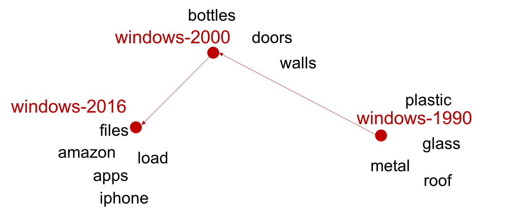
(a) Word “windows”

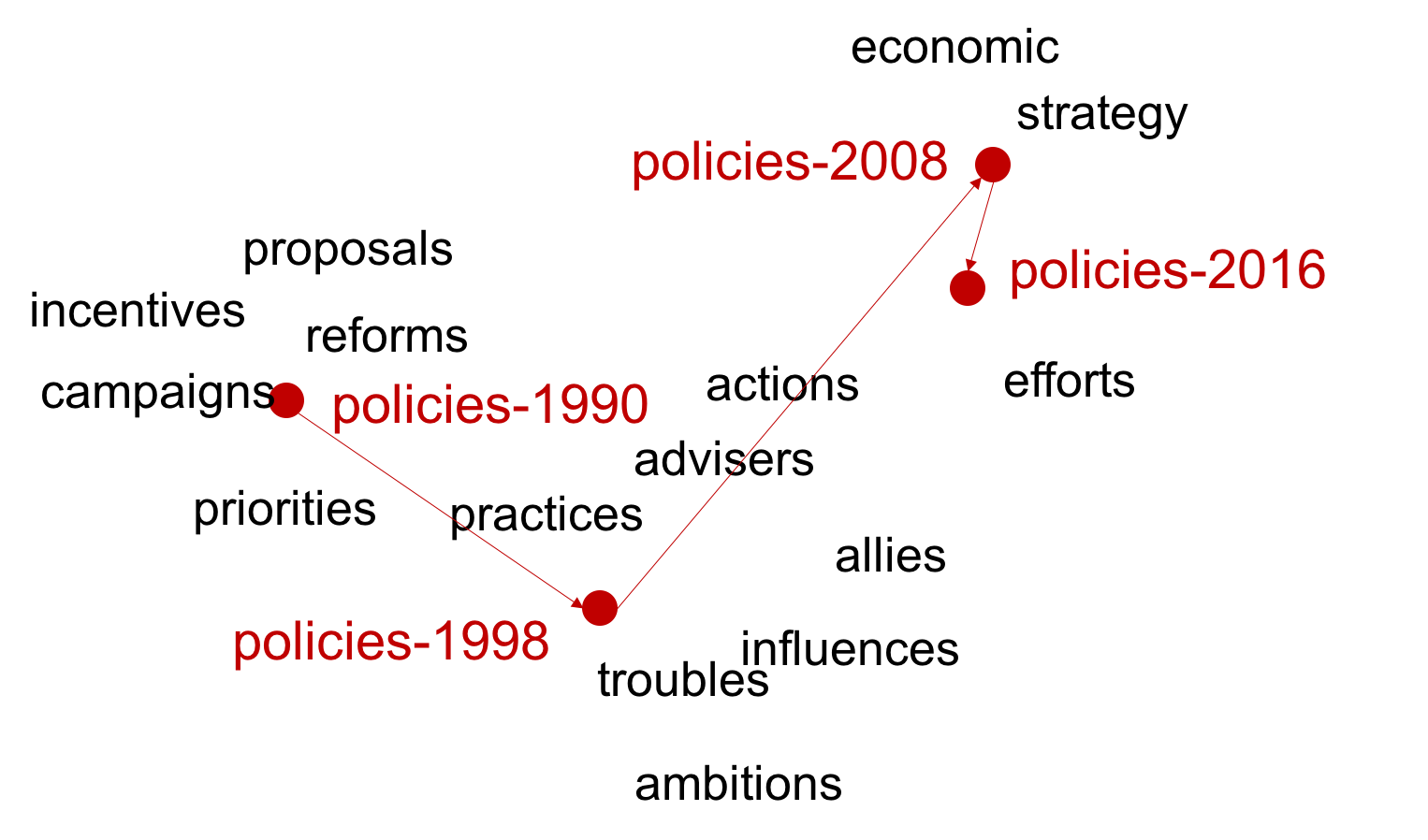
(b) Word “policies”

Figure 2: The trajectory of word embeddings over time.

Different from aligning independently pre-trained embeddings, joint learning of time-stamped embeddings are shown to better capture semantic changes across time. Bamler and Mandt (2017); Yao et al. (2018). Bamler and Mandt uses a probabilistic language model to capture latent trajectories of word vectors across time Bamler and Mandt (2017). Their model is based on Bayesian skip-gram model, a probabilistic variant of word2vec. It learns embeddings $\mathbf{V}^{(t)}$ and context embeddings $\mathbf{U}^{(t)}$ at each time $t$. To align word embeddings across time, they add Gaussian assumption on the evolution of embeddings from time $t$ to $t+1$. They assume that the probability of $\mathbf{U}^{(t+1)}$ conditioned on $\mathbf{U}^{(t)}$, $p(\mathbf{U}^{(t+1)}|\mathbf{U}^{(t)})$, follows Gaussian distribution. This Gaussian constraint prevents embeddings from growing large and enforces smooth vector trajectories.

Yao et al. used matrix factorization to learn an embedding matrix $\mathbf{V}^{(t)}$ and a context embedding matrix $\mathbf{U}^{(t)}$ from PPMI matrix $\mathbf{Y}^{(t)}$ with alignment constraints Yao et al. (2018).

$$\mathbf{U}^{*},\mathbf{V}^{*}=\operatorname*{\arg\!\min}\limits_{\mathbf{U}^{(t)},\mathbf{V}^{(t)}}\frac{1}{2}\sum\limits_{t=1}^{T}\lVert\mathbf{Y}^{(t)}-\mathbf{V}^{(t)}{\mathbf{U}^{(t)}}^{T}\rVert_{F}^{2}$$

$$+\frac{\gamma}{2}\sum\limits_{t=1}^{T}\lVert\mathbf{V}^{(t)}-\mathbf{U}^{(t)}\rVert_{F}^{2}$$

$$+\frac{\lambda}{2}\sum\limits_{t=1}^{T}\lVert\mathbf{V}^{(t)}\rVert_{F}^{2}+\frac{\tau}{2}\sum\limits_{t=2}^{T}\lVert\mathbf{V}^{(t-1)}-\mathbf{V}^{(t)}\rVert_{F}^{2}$$

$$+\frac{\lambda}{2}\sum\limits_{t=1}^{T}\lVert\mathbf{U}^{(t)}\rVert_{F}^{2}+\frac{\tau}{2}\sum\limits_{t=2}^{T}\lVert\mathbf{U}^{(t-1)}-\mathbf{U}^{(t)}\rVert_{F}^{2},$$

where terms $\lVert\mathbf{V}^{(t-1)}-\mathbf{V}^{(t)}\rVert_{F}^{2}$ and $\lVert\mathbf{U}^{(t-1)}-\mathbf{U}^{(t)}\rVert_{F}^{2}$ are alignment constraints on embeddings in neighboring time periods.

The third category of temporal embedding models are built upon pre-trained language models such as BERT Devlin et al. (2018). These models are pre-trained on large corpus to learn representations for words in a given context, which can be taken as the sense embedding. Time-specific word semantics are treated as different senses of words, and thus are represented by the contextualized representations Hu et al. (2019); Giulianelli et al. (2020).

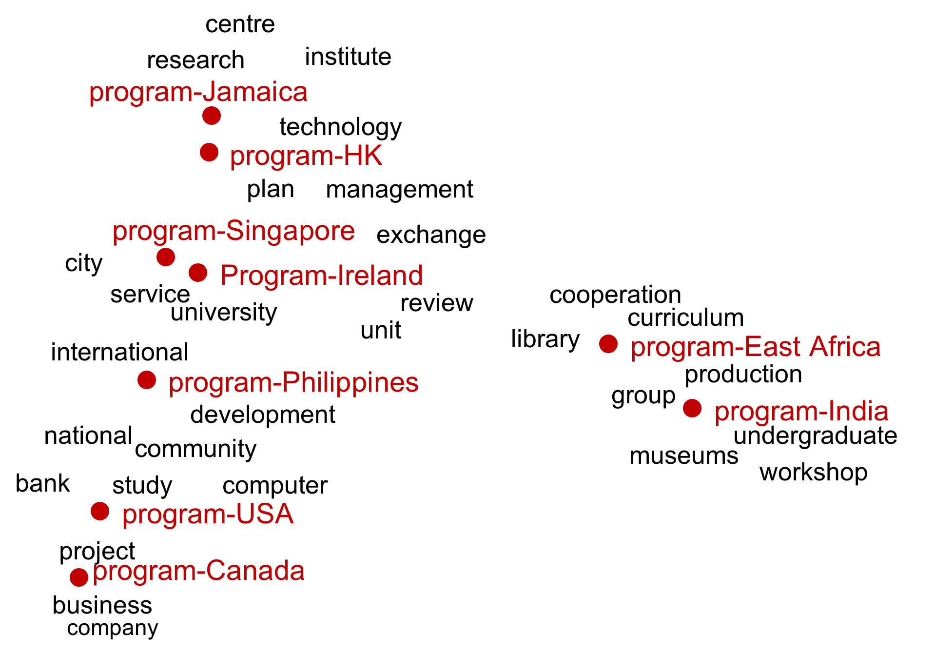
Figure 3: The trajectory of word embeddings over locations.

6.2 Model and Optimization Problem

A model of static word embeddings is proposed by Arora et al., and provides a unified understanding of a group of embedding models including pointwise mutual information (PMI) method, word2vec and GloVe Arora et al. (2016). It reveals that all these models train embeddings to estimate word co-occurrences in the training corpus. Suppose that $\mathbb{P}_{s}(w_{1},w_{2})$ is the co-occurrence probability of words $w_{1}$ and $w_{2}$ in context window of size $s$, $\mathbf{v}_{w_{1}}$ and $\mathbf{v}_{w_{2}}$ are word vectors. Their model states that

$$\log\mathbb{P}_{s}(w_{1},w_{2})=\frac{\lVert\mathbf{v}_{w_{1}}+\mathbf{v}_{w_{2}}\rVert_{2}^{2}}{2d}-2\log Z+\gamma\pm\epsilon,$$ (14)

where $d$ is the embedding dimension, $Z$ is a constant, $\gamma=\log\left(\frac{s(s-1)}{2}\right)$ and $\epsilon$ is an error term. We consider the window size $s$ to be a constant. Since the coefficient $\frac{1}{d}$ can be absorbed as a constant scale of the word vectors, the model suggests the approximation of the logarithm of word co-occurrence probability below:

$$\log\mathbb{P}(w_{1},w_{2})=\frac{1}{2}\lVert\mathbf{v}_{w_{1}}+\mathbf{v}_{w_{2}}\rVert_{2}^{2}+\tau,$$

where constant $\tau=-2\log Z+\gamma$.

We propose a model for condition-specific word embeddings in condition $c$, where $c$ can be time or location.

$$\log\mathbb{P}_{c}(w_{1},w_{2})=\frac{1}{2}\lVert\mathbf{v}_{w_{1},c}+\mathbf{u}_{w_{2},c}\rVert_{2}^{2}+\tau.$$

Since we assume that $\mathbf{v}_{w,c}=\mathbf{v}_{w}\odot\mathbf{q}_{c}+\mathbf{d}_{w,c}$, we can substitute $\mathbf{v}_{w_{1},c}$ with $\mathbf{v}_{w_{1}}\odot\mathbf{q}_{c}+\mathbf{d}_{w_{1},c}$, and substitute $\mathbf{u}_{w_{2},c}$ with $\mathbf{u}_{w_{2}}\odot\mathbf{q}_{c}+\mathbf{d}_{w_{2},c}^{\prime}$. We then have

$$\log\mathbb{P}_{c}(w_{1},w_{2})$$

$$=\frac{1}{2}\lVert(\mathbf{v}_{w_{1}}\odot\mathbf{q}_{c}+\mathbf{d}_{w_{1},c})+(\mathbf{u}_{w_{2}}\odot\mathbf{q}_{c}+\mathbf{d}_{w_{2},c}^{\prime})\rVert^{2}+\tau,$$

$$=\frac{1}{2}\left(\lVert\mathbf{v}_{w_{1}}\odot\mathbf{q}_{c}+\mathbf{d}_{w_{1},c}\rVert^{2}+\lVert\mathbf{u}_{w_{2}}\odot\mathbf{q}_{c}+\mathbf{d}_{w_{2},c}\rVert^{2}\right)$$

$$+(\mathbf{v}_{w_{1}}\odot\mathbf{q}_{c}+\mathbf{d}_{w_{1},c})^{T}(\mathbf{u}_{w_{2}}\odot\mathbf{q}_{c}+\mathbf{d}_{w_{2},c}^{\prime})+\tau,$$

$$=\frac{1}{2}(\lVert\mathbf{v}_{w_{1},c}\rVert^{2}+\lVert\mathbf{u}_{w_{2},c}\rVert^{2}+2\tau)+$$

$$(\mathbf{v}_{w_{1}}\odot\mathbf{q}_{c}+\mathbf{d}_{w_{1},c})^{T}(\mathbf{u}_{w_{2}}\odot\mathbf{q}_{c}+\mathbf{d}_{w_{2},c}^{\prime}).$$ (15)

Here $\frac{1}{2}\lVert\mathbf{v}_{w_{1},c}\rVert^{2}$ can be taken as the bias related to words $w_{1}$ under condition $c$. Similar to GloVe, we introduce a bias term $b_{w_{1},c}$, and $b_{w_{1},c}=\frac{1}{2}\lVert\mathbf{v}_{w_{1},c}\rVert^{2}+\tau$. Similarly, we define bias $b_{w_{2},c}^{\prime}=\frac{1}{2}\lVert\mathbf{v}_{w_{2},c}\rVert^{2}+\tau$.

The logarithm of co-occurrence probability is:

$$\log\mathbb{P}_{c}(w_{1},w_{2})$$

$$=(\mathbf{v}_{w_{1}}\odot\mathbf{q}_{c}+\mathbf{d}_{w_{1},c})^{T}(\mathbf{v}_{w_{2}}^{\prime}\odot\mathbf{q}_{c}+\mathbf{d}_{w_{2},c}^{\prime})$$

$$+b_{w_{1},c}+b_{w_{2},c}^{\prime}.$$ (16)

Our model has two sets of basic word vectors $\{\mathbf{v}_{w}\}$ and $\{\mathbf{u}_{w}\}$, two sets of deviation embeddings $\{\mathbf{d}_{w,c}\}$ and $\{\mathbf{d}_{w,c}^{\prime}\}$, and two sets of bias terms $\{b_{w,c}\}$ and $\{b_{w.c}^{\prime}\}$ for the vocabulary and context vocabulary respectively. All of these parameters are trained to minimize the difference between the real word co-occurrences and the estimated values.

6.3 Word Embedding Trajectory

The trajectories of word windows and policies across time are shown in Fig. 2 (a) and (b). As we can see, windows was commonly used as an opening in houses to allow light and air before the 20th century since its embedding has neighbors such as glass and walls. Recently it also refers to an operating system developed by Microsoft given its neighbors files and load. As for the word policies, it was relevant to campaigns and reforms in 1990, since many campaigns and reforms were launched in that cold-war era. Its meaning has shifted to be relevant to economic over time.

In Fig. 3, we plot the location-specific neighbors of word program. We note that program is a polysemous words with senses including project, software and curriculum. People in one region use it to refer to a sense that is different from another sense used in another region. The different senses can be inferred from its region-specific neighbors. For example, the program is meant as projects or business in Canada, while it is also related to computer software in USA. East Africa and India use it to refer to curriculum in the education domain.

References

- ICE (2019) 2019. International corpus of english. http://ice-corpora.net/ice/. Accessed: 2019-03-12.
- Arora et al. (2016) Sanjeev Arora, Yuanzhi Li, Yingyu Liang, Tengyu Ma, and Andrej Risteski. 2016. A latent variable model approach to pmi-based word embeddings. Transactions of the Association for Computational Linguistics, 4:385–399.
- Bamler and Mandt (2017) Robert Bamler and Stephan Mandt. 2017. Dynamic word embeddings. In International Conference on Machine Learning, pages 380–389.
- Bamman et al. (2014) David Bamman, Chris Dyer, and Noah A Smith. 2014. Distributed representations of geographically situated language. In Proceedings of the 52nd Annual Meeting of the Association for Computational Linguistics, volume 2, pages 828–834.
- Blank (1999) Andreas Blank. 1999. Why do new meanings occur? a cognitive typology of the motivations for lexical semantic change. Historical semantics and cognition, 13:6.
- Brandon Jr (2001) Daniel Brandon Jr. 2001. Localization of web content. Journal of Computing Sciences in Colleges, 17(2):345–358.
- Choi and Varian (2012) Hyunyoung Choi and Hal Varian. 2012. Predicting the present with google trends. Economic Record, 88:2–9.
- Devlin et al. (2018) Jacob Devlin, Ming-Wei Chang, Kenton Lee, and Kristina Toutanova. 2018. Bert: Pre-training of deep bidirectional transformers for language understanding. arXiv preprint arXiv:1810.04805.
- Dubossarsky et al. (2019) Haim Dubossarsky, Simon Hengchen, Nina Tahmasebi, Dominik Schlechtweg, et al. 2019. Time-out: Temporal referencing for robust modeling of lexical semantic change. In The 57th Annual Meeting of the Association for Computational Linguistics (ACL2019) Proceedings of the Conference. ACL.
- Eisenstein et al. (2010) Jacob Eisenstein, Brendan O’Connor, Noah A Smith, and Eric P Xing. 2010. A latent variable model for geographic lexical variation. In Proceedings of the 2010 conference on empirical methods in natural language processing, pages 1277–1287.
- Giulianelli et al. (2020) Mario Giulianelli, Marco Del Tredici, and Raquel Fernández. 2020. Analysing lexical semantic change with contextualised word representations. In Proceedings of the 58th Annual Meeting of the Association for Computational Linguistics, ACL 2020, Online, July 5-10, 2020, pages 3960–3973. Association for Computational Linguistics.
- Gong et al. (2018) Hongyu Gong, Suma Bhat, and Pramod Viswanath. 2018. Embedding syntax and semantics of prepositions via tensor decomposition. In Proceedings of the 2018 Conference of the North American Chapter of the Association for Computational Linguistics: Human Language Technologies, Volume 1 (Long Papers), pages 896–906.
- Gong et al. (2017) Hongyu Gong, Jiaqi Mu, Suma Bhat, and Pramod Viswanath. 2017. Prepositions in context. arXiv preprint arXiv:1702.01466.
- Hamilton et al. (2016) William L Hamilton, Jure Leskovec, and Dan Jurafsky. 2016. Diachronic word embeddings reveal statistical laws of semantic change. In Proceedings of the 54th Annual Meeting of the Association for Computational Linguistics, pages 1489–1501.
- Hu et al. (2019) Renfen Hu, Shen Li, and Shichen Liang. 2019. Diachronic sense modeling with deep contextualized word embeddings: An ecological view. In Proceedings of the 57th Annual Meeting of the Association for Computational Linguistics, pages 3899–3908.
- Huang and Paul (2019) Xiaolei Huang and Michael Paul. 2019. Neural temporality adaptation for document classification: Diachronic word embeddings and domain adaptation models. In Proceedings of the 57th Annual Meeting of the Association for Computational Linguistics, pages 4113–4123.
- Kachru et al. (2006) Braj B Kachru, Yamuna Kachru, Cecil L Nelson, Daniel R Davis, and Zoya G Proshina. 2006. The handbook of world Englishes. Wiley Online Library.
- Kulkarni et al. (2015) Vivek Kulkarni, Rami Al-Rfou, Bryan Perozzi, and Steven Skiena. 2015. Statistically significant detection of linguistic change. In Proceedings of the 24th International Conference on World Wide Web, pages 625–635.
- Kulkarni et al. (2016) Vivek Kulkarni, Bryan Perozzi, and Steven Skiena. 2016. Freshman or fresher? quantifying the geographic variation of language in online social media. In Tenth International AAAI Conference on Web and Social Media.
- Kutuzov et al. (2018) Andrey Kutuzov, Lilja Øvrelid, Terrence Szymanski, and Erik Velldal. 2018. Diachronic word embeddings and semantic shifts: a survey. In Proceedings of the 27th International Conference on Computational Linguistics, pages 1384–1397.
- Lijffijt et al. (2012) Jefrey Lijffijt, Tanja Säily, and Terttu Nevalainen. 2012. Ceecing the baseline: Lexical stability and significant change in a historical corpus. In Studies in Variation, Contacts and Change in English, volume 10.
- Mesthrie and Bhatt (2008) Rajend Mesthrie and Rakesh M Bhatt. 2008. World Englishes: The study of new linguistic varieties. Cambridge University Press.
- Michel et al. (2011) Jean-Baptiste Michel, Yuan Kui Shen, Aviva Presser Aiden, Adrian Veres, Matthew K Gray, Joseph P Pickett, Dale Hoiberg, Dan Clancy, Peter Norvig, Jon Orwant, et al. 2011. Quantitative analysis of culture using millions of digitized books. science, 331(6014):176–182.
- Mikolov et al. (2013) Tomas Mikolov, Ilya Sutskever, Kai Chen, Greg S Corrado, and Jeff Dean. 2013. Distributed representations of words and phrases and their compositionality. In Advances in neural information processing systems, pages 3111–3119.
- Pennington et al. (2014) Jeffrey Pennington, Richard Socher, and Christopher Manning. 2014. Glove: Global vectors for word representation. In Proceedings of the 2014 conference on empirical methods in natural language processing (EMNLP), pages 1532–1543.
- Peters et al. (2018) Matthew Peters, Mark Neumann, Mohit Iyyer, Matt Gardner, Christopher Clark, Kenton Lee, and Luke Zettlemoyer. 2018. Deep contextualized word representations. In NAACL 2018, volume 1, pages 2227–2237.
- Poirier (2014) Éric André Poirier. 2014. A method for automatic detection and manual localization of content-based translation errors and shifts. Journal of Innovation in Digital Ecosystems, 1(1-2):38–46.
- Qi et al. (2018) Ye Qi, Devendra Sachan, Matthieu Felix, Sarguna Padmanabhan, and Graham Neubig. 2018. When and why are pre-trained word embeddings useful for neural machine translation? In NAACL 2018, volume 2, pages 529–535.
- Rosenfeld and Erk (2018) Alex Rosenfeld and Katrin Erk. 2018. Deep neural models of semantic shift. In Proceedings of the 2018 Conference of the North American Chapter of the Association for Computational Linguistics: Human Language Technologies, pages 474–484.
- Roweis and Saul (2000) Sam T Roweis and Lawrence K Saul. 2000. Nonlinear dimensionality reduction by locally linear embedding. science, 290(5500):2323–2326.
- Schlechtweg et al. (2020) Dominik Schlechtweg, Barbara McGillivray, Simon Hengchen, Haim Dubossarsky, and Nina Tahmasebi. 2020. Semeval-2020 task 1: Unsupervised lexical semantic change detection. arXiv preprint arXiv:2007.11464.
- Silva-Corvalán (2006) Carmen Silva-Corvalán. 2006. Analyzing linguistic variation: Statistical models and methods. Journal of Linguistic Anthropology, 16(2):295–296.
- Tang (2018) Xuri Tang. 2018. A state-of-the-art of semantic change computation. Natural Language Engineering, 24(5):649–676.
- Ullmann (1979) Stephen Ullmann. 1979. Semantics: an introduction to the science of meaning.
- Yao et al. (2018) Zijun Yao, Yifan Sun, Weicong Ding, Nikhil Rao, and Hui Xiong. 2018. Dynamic word embeddings for evolving semantic discovery. In Proceedings of the Eleventh ACM International Conference on Web Search and Data Mining, pages 673–681. ACM.
- Zhang et al. (2016) Yating Zhang, Adam Jatowt, Sourav S Bhowmick, and Katsumi Tanaka. 2016. The past is not a foreign country: Detecting semantically similar terms across time. IEEE Transactions on Knowledge and Data Engineering, 28(10):2793–2807.