Transients generate memory and break hyperbolicity in stochastic enzymatic networks

Abstract

The hyperbolic dependence of catalytic rate on substrate concentration is a classical result in enzyme kinetics, quantified by the celebrated Michaelis-Menten equation. The ubiquity of this relation in diverse chemical and biological contexts has recently been rationalized by a graph-theoretic analysis of deterministic reaction networks. Experiments, however, have revealed that “molecular noise” - intrinsic stochasticity at the molecular scale - leads to significant deviations from classical results and to unexpected effects like “molecular memory”, i.e., the breakdown of statistical independence between turnover events. Here we show, through a new method of analysis, that memory and non-hyperbolicity have a common source in an initial, and observably long, transient peculiar to stochastic reaction networks of multiple enzymes. Networks of single enzymes do not admit such transients. The transient yields, asymptotically, to a steady-state in which memory vanishes and hyperbolicity is recovered. We propose new statistical measures, defined in terms of turnover times, to distinguish between the transient and steady states and apply these to experimental data from a landmark experiment that first observed molecular memory in a single enzyme with multiple binding sites. Our study shows that catalysis at the molecular level with more than one enzyme always contains a non-classical regime and provides insight on how the classical limit is attained.

I Introduction

The Michaelis-Menten equation, describing the hyperbolic dependence of the rate of catalysis on the substrate concentration, is a classical result in enzyme kinetics key-1 . It was derived by Michaelis and Menten in 1913 for a network of three elementary reactions, $E+S\rightleftharpoons ES\rightarrow E+P,$ describing the reversible binding of enzyme $E$ with substrate $S$ to form complex $ES$ and its irreversible dissociation into product $P$ and regenerated enzyme $E$ key-2 ; key-3 ; key-4 . The hyperbolic dependence of catalytic rate on substrate concentration is found to hold in enzymatic networks of far greater complexity. It implies a linear relation between the inverse catalytic rate and the inverse substrate concentration and, in this form, is widely used to estimate rate parameters and infer mechanisms from kinetic data key-8 . The surprising ubiquity of this equation in chemical and biological processes has recently been rationalized by a graph-theoretical analysis of complex, deterministic, reaction networks key-9 .

At the molecular level, however, enzymatic reactions do not proceed deterministically key-10 ; key-11 ; key-12 ; key-13 ; key-14 . Fluctuations, of both quantum mechanical and thermal origin, termed “molecular noise”, influence each step of a chemical reaction, such that neither the lifetime of a chemical state nor the state to which it transits can be known with certainty key-15 ; key-16 ; key-17 . Further, the discrete change in the reactant numbers is comparable to the number of reacting molecules, and a description in terms of continuously varying concentrations is inadmissible key-15 ; key-16 ; key-17 ; key-58 (15, 16). In the limit of large numbers of reactants, when both fluctuations and the change in reactants compared to their total number are small, a deterministic description in terms of continuously varying concentrations is recovered key-18 (16). The Michaelis-Menten equation is obtained when, in addition, there is a separation of time scales between the (rapid) equilibration between enzyme and complex and (slow) product formation key-2 . This rapid equilibrium approximation is a special case of the steady-state approximation (SSA), in which the rates of complex formation and dissociation are assumed to be equal, as noted by Briggs and Haldane key-56 (17).

The first theoretical study of catalytic fluctuations was undertaken by Bartholomay half a century after the discovery of the Michaelis-Menten (MM) equation key-18 (16). His principal contribution was to show that discrete-state continuous-time Markov processes provide a mathematical framework that incorporates the discrete change in molecular numbers, the effect of molecular noise in each reaction step, and reactions mechanisms of arbitrary complexity. The classical rate equations for concentrations were thus replaced by chemical “master equations” for the probabilities of the (non-negative) number of reactants. Bartholomay obtained the mean and variance of these for the Michaelis-Menten mechanism $E+S\rightleftharpoons ES\rightarrow E+P$. The apparent irreproducibility of experiments that measured the rate of change of concentrations was recognized to be a fluctuation effect and a method was suggested to estimate the rate constraints from the variances of the concentrations.

The long hiatus of interest that followed this pioneering work was brought to a close by a landmark experiment that directly observed catalytic fluctuations at the single-molecule level key-12 ; key-13 . As concentrations are not defined for a single molecule, the experiment measured, instead, the times at which the enzyme yielded products, one product at a time. This time series data was analyzed in terms of the interval between consecutive turnovers, defined to be the “waiting time”. For repeated experiments under identical conditions, the waiting times showed a distribution and this was attributed to the effect of molecular noise. The analysis of waiting time distributions revealed several remarkable facts. First, the distribution changed character with increase in substrate concentration, from a single exponential to one that was not. Second, the inverse of the mean waiting time obeyed the MME at low substrate concentrations. Third, the randomness parameter, the ratio of the variance to the squared mean, was a monotonically increasing function of the substrate concentration, bounded below by one. Fourth, the waiting times between consecutive turnovers were found to be statistically dependent, with substantial positive correlations, an effect termed “molecular memory”. Subsequent experiments in single-nanoparticle catalysis confirmed these empirical facts and established their generality key-57 (18, 19, 20). While it was understood that these seemingly disparate observations have their origin in molecular noise, the precise manner in which they emerge from underlying molecular fluctuations and how they are influenced by different reaction mechanisms was not elucidated.

The central theoretical question that needs to be answered in rationalizing such single-molecule temporal data is this: can we derive the statistics of temporal fluctuations from the chemical master equation, incorporating discreteness, molecular noise, and reaction mechanisms, in the manner that the statistics of number fluctuations was derived by Bartholomay? Here we present a formalism that permits us to answer this question affirmatively. Using this formalism we are able to make a direct connection between reaction mechanisms and the statistics of waiting times and, thus, explain their puzzling features from a unified point of view.

In Section II we consider a generic stochastic enzymatic reaction network, incorporating conformational fluctuations and parallel pathways to product formation, and present the corresponding chemical master equation (CME). We marginalize the reactant probabilities to obtain the probability of there being $n$ turnovers at any given time and present several experimentally relevant summary statistics. We introduce the probability distributions of the turnover and waiting times and present their relevant summary statistics. We then derive an expression that connects the reactant probabilities of the CME to the distribution of waiting times. This provides the sought after link between the description in terms of waiting times (“point process”) key-21 (21), in which experimental data is naturally recorded, and the description in terms of reactant numbers (“counting process”) key-22 (22), through which mechanisms are most conveniently expressed.

In Section III we apply this formalism to study a reaction network corresponding to a single enzyme. In such a network, reactant numbers are either zero or one, and a non-zero value of one reactant number implies zero values of all others. We explore the consequences of this “fermionic” character and find that, irrespective of the complexity of the network, turnovers are always statistically independent and identically distributed, or, in other words, constitute a renewal process key-23 (23). A single-enzyme network, then, cannot show molecular memory.

In Section IV we consider a network consisting of replicas of single-enzyme networks, corresponding to oligomeric enzymes with independent and identical binding sites. The absence of “fermionic” character in these networks permits turnovers to be statistically dependent and allows them to show molecular memory. The statistical dependence decreases with the number of turnovers and vanishes asymptotically. We characterize this transient with fading memory through the conditional distribution of consecutive turnovers, which we relate to measures of the single-enzyme network. This analysis explains the counter-intuitive appearance of memory in a process whose elementary steps, recalling that the CME describes a Markov process, are memoryless.

In Section V we discuss new statistical measures that, contrary to existing measures key-24 (24, 25, 26), do not assume the statistical independence of turnovers. Our measures, then, can be applied uniformly over the entire duration of the catalytic process, both in the transient state with memory and the steady state in which memory vanishes. We provide an expression for the enzymatic velocity in terms of turnover times that reduces to the classical expression in the thermodynamic limit and elucidates how this limit is reached.

In Section VI we compare our theory with the classic experiment on $\beta$-galactosidase key-12 , a tetrameric enzyme, and find excellent agreement with four replicas of a single-enzyme network with conformers and parallel pathways. Saliently, we do not need to assume any ad-hoc distribution of reaction rates key-27 (27, 28): the “dynamic disorder” implied by such a distribution is an emergent feature of our theory.

We conclude, in section VII, with a discussion on how our theory can be extended to non-replica networks corresponding to enzymes with interacting binding sites.

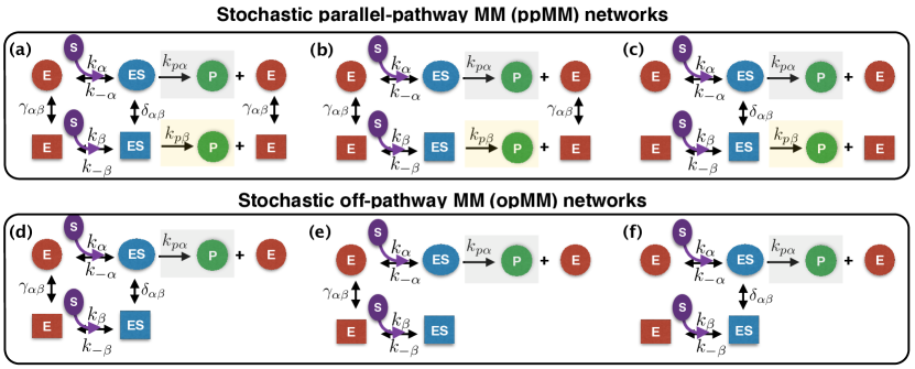
Figure 1: Enzymatic networks for a single catalytic site, including conformational fluctuations and parallel pathways to product formation. The general network in (a) reduces to the special cases in (b) through (f) when rate constants for the corresponding steps are set to zero.

II Stochastic enzymatic networks

The stochastic description of chemical reactions begins with a set of $k$ non-negative integers $\boldsymbol{n}=(n_{1},\ldots,n_{k})$ describing the number of molecules of the $k$-th species. Elementary reactions

$$\sigma\text{-th reaction step}:\,\,\,\boldsymbol{n}\underset{t_{\sigma}^{\leftarrow}}{\stackrel{{\scriptstyle t_{\sigma}^{\rightarrow}}}{{\rightleftharpoons}}}\boldsymbol{n}+\boldsymbol{r}_{\sigma}$$ (1)

labelled by the index $\sigma$, take the state $\boldsymbol{n}$ to the state $\boldsymbol{n}+\boldsymbol{r}_{\sigma}$ where $\boldsymbol{r}_{\sigma}$ is a vector representing the integer changes of each species, as determined by the reaction stoichiometry. The probability per unit time that this reaction takes place is $t_{\sigma}^{\rightarrow}(\boldsymbol{n})$. The corresponding backward reaction takes the state $\boldsymbol{n}+\boldsymbol{r}_{\sigma}$ to the state $\boldsymbol{n}$ at the rate $t_{\sigma}^{\leftarrow}(\boldsymbol{n}+\boldsymbol{r}_{\sigma})$. The rates are combinatoric functions that follow from the law of mass action. The probability $P(\boldsymbol{n},t)$ of being in the state $\boldsymbol{n}$ at time $t$ is governed by the CME key-22 (22, 29, 16)

$$\partial_{t}P(\boldsymbol{n}) =\sum_{\sigma}t_{\sigma}^{\rightarrow}(\boldsymbol{n}-\boldsymbol{r}_{\sigma})P(\boldsymbol{n}-\boldsymbol{r}_{\sigma})-t_{\sigma}^{\leftarrow}(\boldsymbol{n})P(\boldsymbol{n})$$

$$+\sum_{\sigma}t_{\sigma}^{\leftarrow}(\boldsymbol{n}+\boldsymbol{r}_{\sigma})P(\boldsymbol{n}+\boldsymbol{r}_{\sigma})-t_{\sigma}^{\rightarrow}(\boldsymbol{n})P(\boldsymbol{n})$$ (2)

which is a system of coupled ordinary differential equations, equal in number to the number of distinct states of the network.

Here, we consider enzymatic networks that contain the Michaelis-Menten mechanism $E_{i}+S\rightleftharpoons ES_{i}\rightarrow E_{i}+P$ as a basic motif while allowing for conformers $i=\alpha,\beta,\ldots$ and parallel pathways to product formation key-12 ; key-13 . The state is described by the vector $\boldsymbol{n}=(n_{E_{\alpha}},n_{ES_{\alpha}},n_{E_{\beta}},n_{ES_{\beta}},\ldots,n)$ of non-negative integers comprising of, in obvious notation, the numbers of enzyme and complex, of each conformational type, and of product. Examples of such networks for the simplest case of two conformers are shown in Fig.(1) for both parallel and off-pathway kinetics key-30 (30). The corresponding rates are listed in Table. (1). The bimolecular complexation steps are replaced by pseudo-unimolecular steps with effective rate constants denoted by primes. All rates are then linear in the state vector $\boldsymbol{n}$. It is important to note that the rates do not depend on the number of products.

Step	$\boldsymbol{r}_{\sigma}$	$t_{\sigma}^{\rightarrow}(\boldsymbol{n})$	$t_{\sigma}^{\leftarrow}(\boldsymbol{n})$
$E_{\alpha}\rightleftharpoons E{}_{\beta}$	$(-1,0,1,0,0)$	$\gamma_{\alpha\beta}n_{E_{\alpha}}$	$\gamma_{\alpha\beta}n_{E_{\beta}}$
$ES_{\alpha}\rightleftharpoons ES_{\beta}$	$(0,-1,0,1,0)$	$\delta_{\alpha\beta}n_{ES_{\alpha}}$	$\delta_{\alpha\beta}n_{ES_{\beta}}$
$E_{\alpha}\rightleftharpoons ES_{\alpha}$	$(-1,1,0,0,0)$	$k_{\alpha}^{\prime}n_{E_{\alpha}}$	$k_{-\alpha}n_{ES_{\alpha}}$
$E_{\beta}\rightleftharpoons ES_{\beta}$	$(0,0,-1,1,0)$	$k_{\beta}^{\prime}n_{E_{\beta}}$	$k_{-\beta}n_{ES_{\beta}}$
$ES_{\alpha}\rightarrow P+E{}_{\alpha}$	$(1,-1,0,0,1)$	$k_{p\alpha}n_{ES_{\alpha}}$	$0$
$ES_{\beta}\rightarrow P+E{}_{\beta}$	$(0,0,1,-1,1)$	$k_{p\beta}n_{ES_{\beta}}$	$0$

Table 1: Elementary reaction steps and their rates for the single-site network labelled (a) in Fig. (1). The networks labelled (b) through (c) are obtained by setting corresponding rate parameters to zero. The forward reaction takes the state $\boldsymbol{n}=(n_{E_{\alpha}},n_{ES_{\alpha}},n_{E_{\beta}},n_{ES_{\beta}},n)$ to the state $\boldsymbol{n}+\boldsymbol{r}_{\sigma}$. The pseudo-first-order rate constants for the forward reaction are $k_{\alpha}^{\prime}=k_{\alpha}[S]$ and $k_{\beta}^{\prime}=k_{\beta}[S]$. All rates are independent of the number of products $n$.

It is convenient to partition the state vector into $\boldsymbol{n}=(\boldsymbol{n}^{\star},n)$, where $\boldsymbol{n}^{\star}=(n_{E_{\alpha}},n_{ES_{\alpha}},n_{E_{\beta}},n_{ES_{\beta}},\ldots)$ are “hidden” state components unobserved in experiment, and $n$ is the “observed” product state visible through fluorescence bursts. The hidden state vector has $2l$ components in a network with $l$ conformers. For a network with $\nu$ enzymes, or one oligomeric enzyme with $\nu$ active sites, mass conservation implies that the sum of the number of enzymes in the uncomplexed and complexed states must sum to $\nu$: $n_{E_{\alpha}}+n_{E_{\beta}}+\ldots+n_{ES_{\alpha}}+n_{ES_{\beta}}+\ldots=\nu$. For a single enzyme (or active site), this implies that $n_{E_{\alpha}}+n_{E_{\beta}}+\ldots+n_{ES_{\alpha}}+n_{ES_{\beta}}+\ldots=1$. Therefore, the components of the hidden state vector in a single-enzyme network have a “fermionic” character, where the components only take the values zero or one and only one component is non-zero at any point in time. Mass conservation also implies that the number of hidden states is finite and equal to the number of compositions of $\nu$ into $l$ parts. For a single enzyme with $l$ conformers, this gives $2l$ states. We shall return to this important property below.

Unlike the hidden components, the number of products $n$ can take values from zero to infinity. The probability of their being $n$ products at time $t$ is obtained by marginalizing the reactant probability over the hidden states,

$$P(n,t)=\sum_{\boldsymbol{n}^{\star}}P(\boldsymbol{n},t).$$ (3)

This is the fundamental probability distribution in the counting process description of turnovers. The expectation with respect to this probability distribution of the mean and variance of $n$ define the enzymatic velocity and Fano factor key-31 (31),

$$V(t)=\frac{d}{dt}\langle n\rangle,\quad\rho(t)=\frac{\langle n^{2}\rangle-\langle n\rangle^{2}}{\langle n\rangle}\quad(t\geq 0)$$ (4)

Such quantities have been calculated for a variety of networks beginning with the work of Bartholomay. However, as mentioned in the Introduction, they are not directly relevant to single-enzyme experiments which record the times $T_{p}$ at which turnovers occur, rather than the number of turnovers at time $t$. Here $p=1,2,\cdots$ is the turnover number index. This motivates the study of the point process of turnovers, for which we now introduce the fundamental probability distributions key-21 (21).

We define the turnover time for the $p$-th product, $T_{p},$ to be the smallest value of $t$ such that $n\geq p$, or more precisely, $T_{p}=\text{inf}\{t>0:n(t)\geq p\}$. The cumulative distribution of the $p$-th turnover time $T_{p}$ is denoted by $P(T_{p}\leq t)$. This defines the survival probability $P(T_{p}>t)=1-P(T_{p}\leq t)$ and probability density $w_{T_{p}}(t)dt=P(t<T_{p}\leq t+dt)$. The expectation of $T_{p}$ with respect to the probability density defines the mean turnover time and the randomness parameter for the $p$-th turnover,

$$\mu_{p}=\langle T_{p}\rangle,\quad r_{p}=p\frac{\langle T_{p}^{2}\rangle-\langle T_{p}\rangle^{2}}{\langle T_{p}\rangle^{2}}\quad(p=1,2,\ldots)$$ (5)

While the current definition of the randomness parameter is $p$ independent $r=\langle\tau^{2}\rangle-\langle\tau\rangle^{2}/\langle\tau\rangle^{2}$ key-32 (32, 33), the factor of $p$ in the above definition of the randomness parameter is introduced for reasons that will become apparent in Section V. Higher moments can be studied but, to the best of our knowledge, have not been measured in experiment.

To quantify statistical dependences, it is convenient to define the waiting time between turnovers,

$$\tau_{p}=T_{p}-T_{p-1},$$ (6)

and study their joint density distributions, $w(\tau_{1},\tau_{2},\ldots)$. The marginal distributions $w(\tau_{p})$ describe the statistics of individual turnovers while the joint distributions $w(\tau_{p},\tau_{q})$ describe the statistics of pairs of turnovers. It is convenient to write this joint distribution as

$$w(\tau_{p},\tau_{q})=w(\tau_{p})g(\tau_{p},\tau_{q})w(\tau_{q})$$ (7)

so that statistical dependences are contained in $g(\tau_{p},\tau_{q})$. Pairs of turnovers are statistically independent if and only if $g(\tau_{p},\tau_{q})=1$ for all $p$ and $q$. The correlation function

$$C_{pq}=\langle\tau_{p}\tau_{q}\rangle=c(\tau_{p},\tau_{q})\langle\tau_{p}\rangle\langle\tau_{q}\rangle$$ (8)

serves as a second-order statistic for identifying statistical dependences. The expectations are with respect to the joint distribution $w(\tau_{p},\tau_{q}).$ Statistical dependences and molecular memory imply $c(\tau_{p},\tau_{q})\neq 1$.

The question naturally arises as to how the probability distributions for the counting process, $P(n,t)$, and the point process, $P(T_{p}\leq t)$, together with their summary statistics, are related to each other and to the underlying CME which is the generative process that underlies both distributions. We provide the answer below.

From the definitions of the random variables $n$ and $T_{p}$, it is clear that at any time $t$,

$$T_{p}\leq t\Longleftrightarrow n(t)\geq p$$ (9)

or, in other words, these two events are equal in probability. Since the event $n(t)<p$ is their complement, we have

$$P(T_{p}\leq t)=P(n\geq p,t)=1-P(n<p,t).$$ (10)

Since the product states are mutually exclusive, we have $P(n<p,t)=\sum_{n=0}^{p-1}P(n,t)$. Combining this with the marginal expression for $P(n,t)$ we obtain

$$P(T_{p}\leq t)=1-\sum_{n=0}^{p-1}\sum_{\boldsymbol{n}^{\star}}P(\boldsymbol{n},t).$$ (11)

This relation between the turnover time distribution and the solution of the CME is the central result of this section. It is applicable to networks of arbitrary complexity and provides the sought after connection between the statistics of turnovers and reaction mechanisms. The probability density follows upon differentiation,

$$w_{T_{p}}(t)=-\sum_{n=0}^{p-1}\sum_{\boldsymbol{n}^{\star}}\partial_{t}P(\boldsymbol{n},t),$$ (12)

and is often more convenient for comparison with experimental data, when the latter is presented in the form of a probability density. A special case of this relation was first obtained in key-15 .

We have not been able to find a relation of this generality that relates the waiting time distributions $w(\tau_{p})$ and $w(\tau_{p},\tau_{q})$ to the solution of the CME. However, in particular instances, where the network is “fermionic” or has a “replica” character, relations to the underlying CME can be found, as we show in Sections III and IV, respectively.

III Renewal statistics in single-enzyme networks

As we noted above, hidden states in a single-enzyme network have a “fermionic” character: the components of the hidden state vector can only take the values zero or one, and only one component can be non-zero at any time. This implies that immediately after the conclusion of a turnover, say the $p$-th, the network is in a state corresponding to a single uncomplexed enzyme. To elaborate, consider the MM network with state vector $\boldsymbol{n}=(n_{E},n_{ES},n)$ and hidden state vector $\boldsymbol{n}^{\star}=(n_{E},n_{ES})$. The two allowed hidden states are $(1,0)$ and $(0,1)$ corresponding to uncomplexed and complexed enzyme. Labeling these by $E$ and $ES$, the allowed states of the network are $(E,n)$ and $(ES,n)$. At the conclusion of the $p$-th turnover at $t=T_{p}$ the network is in the state $(E,p)$ and so, taking limits from above,

$$\lim_{t\rightarrow T_{p}^{+}}P(E,p,t)=1.$$ (13)

For the two-conformer ppMM network with state vector $\boldsymbol{n}=(n_{E_{\alpha}},n_{ES_{\alpha}},n_{E_{\beta}},n_{ES_{\beta}},n)$ and hidden state vector $\boldsymbol{n}^{\star}=(n_{E_{\alpha}},n_{ES_{\alpha}},n_{E_{\beta}},n_{ES_{\beta}})$ the four allowed hidden states are $(1,0,0,0)$, $(0,1,0,0),$ $(0,0,1,0)$ and $(0,0,0,1)$. Labeling thse by $E_{\alpha},$ $ES_{\alpha}$, $E_{\beta}$ and $ES_{\beta}$ , the allowed states of the network are $(E_{\alpha},n)$, $(ES_{\alpha},n),$ $(E_{\beta},n)$ and $(ES_{\beta},n)$. At the conclusion of the $p$-th turnover, the network is either in the state $(E_{\alpha},p)$ or in the state $(E_{\beta},p)$ and so

$$\lim_{t\rightarrow T_{p}^{+}}P(E_{\alpha},p,t)+P(E_{\beta},p,t)=1$$ (14)

More generally, for any single-enzyme network the states can be labelled by the conformation of the enzyme and the number of products and at the conclusion of a turnover, the network is surely in one of the uncomplexed states with the total probability is partitioned between those states. As we show below, this recurrent return to a fixed subset of the hidden states, together with the structure of the CME for such networks, implies that conditioning on a turnover makes the future independent of the past. This results in turnovers that are statistically independent, with waiting time distributions that are identically distributed. Single-enzyme turnovers, therefore, form a renewal process and cannot show memory key-23 (23).

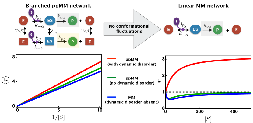
Figure 2: Distinction between the summary statistics of branched and single pathway stochastic networks as a function of substrate concentration. Top panel shows how a parallel-pathway MM (ppMM) network reduces to a single-pathway MM network when conformational fluctuations are disallowed. Bottom left panel shows the single-enzyme Lineweaver-Burk plot for the variation of inverse single-enzyme velocity, $\langle\tau\rangle$, with $1/[S]$. The plot is linear, and thus the variation of single-enzyme velocity with $[S]$ is hyperbolic, irrespective of the network complexity. Bottom right panel shows how the variation of the randomness parameter $r$ with $[S]$ provides a quantitative measure to discern single-enzyme network topologies. For the ppMM network, the rate constants conditions that favor parallel-pathway for product formation can yield $r\geq 1$ (dynamic disorder). The rate constant conditions that disallow the latter always yield $r\leq 1$. For a linear MM network, irrespective of the rate parameter conditions, there is no dynamic disorder as $r$ does not exceed one.

In the absence of memory, attention can be focussed entirely on the statistics of the waiting time, which, since it is identically distributed for all $p,$ we simply denote by $\tau$. We summarize our two main results before providing explicit results for the MM and ppMM networks. First, we show that for a model with $l$ conformers the waiting time distribution is a sum of $2l$ exponentials whose time constants are eigenvalues of a $2l\times 2l$ matrix related to the CME. The behavior of the waiting time distribution is related to the spacing of these eigenvalues. For well-separated eigenvalues, the exponential with the lowest time constant is dominant, but for closely spaced eigenvalues all the $2l$ exponentials contribute. This multi-exponentiality leads to variances that are large compared to the squared mean and, hence, to a randomness parameter that exceeds unity. Our analysis thus transparently relates “dynamic disorder” to reaction mechanisms with fixed rate constants, in contrast to fluctuating rate parameters key-27 (27, 28). Second, we show that the randomness parameter for $\tau$ is a sensitive measure of network topology. It is known that a Markov chain comprising of a linear network of arbitrary complexity always yields $r\leq 1$, bounded below by the inverse of the number of rate determining steps $\sigma$: $r\geq\frac{1}{\sigma}$ key-34 (34). The minimum is attained for a linear sequence of states with equal rate constants, first studied by Erlang key-35 (35). For a single step reaction or a linear network with a single rate determining step, thus, $r=1$. We find that a branched topology is necessary, but not sufficient, to obtain $r>1$. Our explicit calculation for the ppMM network shows that $r$ can vary continuously from $r<1$ to $r>1$ as the substrate concentration is increased. Thus, networks can be rationally designed to yield a desired value of the randomness parameter.

Consider, now, the CME for the MM network, written in terms of the labels $E$,$ES$, and $n$:

$$\partial_{t}P(E,n) =-k_{a}P(E,n)+k_{-1}P(ES,n)+k_{2}P(ES,n-1)$$

$$\partial_{t}P(ES,n) =+k_{a}P(E,n)-k_{-1}P(ES,n)-k_{2}P(ES,n),\quad\quad n=0,1,2,\ldots$$ (15)

It is understood that states with $n<0$ have zero probability. This is an infinite system of autonomous linear differential equations whose solution can be obtained using the technique of generating functions. A great simplification results when we recognize the following two features. First, conditioning the system on the $p-$th turnover at $t=T_{p}$ collapses the probability on the state $(E,p)$ so that $P(E,p)=1$ and all other probabilities are zero. Since probabilities only flow into states with increasing number of products, this implies that probabilities of all states with $n<p$ remain zero subsequently. The future is made conditionally independent of the past. Second, the distribution of the $(p+1)$-th turnover $T_{p+1}$, conditioned on the $p-$th turnover at $T_{p}$, is governed by the same set of equations and initial conditions as the first turnover $T_{1}$, conditioned on the initial state at $t=0$. This implies that $T_{1}$ and $T_{p+1}-T_{p}$ are equal in distribution for all $p$. Therefore, the waiting times $\tau_{p}$ are independent and distributed identically to $T_{1}$.

From Eq. (11) the cumulative distribution of $T_{1}$ is

$$P(T_{1}<t)=1-[P(E,0,t)+P(ES,0,t)]$$ (16)

and from the CME these two probabilities obey

$$\left[\begin{array}[]{c}\partial_{t}P(E,0,t)\\ \partial_{t}P(ES,,0,t)\end{array}\right]=\left[\begin{array}[]{cc}-k_{1}^{\prime}&k_{-1}\\ k_{1}^{\prime}&-(k_{-1}+k_{2})\end{array}\right]\left[\begin{array}[]{c}P(E,0,t)\\ P(ES,0,t)\end{array}\right]$$

with initial condition $P(E,0)=1$ and $P(ES,0)=0$ at $t=0.$ This is a system of ordinary differential equations for the vector $\boldsymbol{P}(t)=[P_{E}(t),P_{ES}(t)]$ , where $P(E,0,t)$ is abbreviated as $P_{E}(t)$ etc, with system matrix

$$\boldsymbol{L}=\exp\left[\begin{array}[]{cc}-k_{1}^{\prime}t&k_{-1}t\\ k_{1}^{\prime}t&-(k_{-1}+k_{2})t\end{array}\right].$$

The solution is obtained in terms of the matrix exponential as $\boldsymbol{P}(t)=\exp(\boldsymbol{L}t)\cdot\boldsymbol{P}(0)$ with the explicit result,

$$P_{E}(t)= \frac{1}{2A}\left[(A+B-C)e^{-(B+A)t}+(A-B+C)e^{-(B-A)t}\right]$$

$$P_{ES}(t)= \frac{k_{1}^{\prime}}{2A}\left[e^{-(B-A)t}-e^{-(B+A)t}\right],$$

where $k_{1}^{\prime}=k_{1}[S]$, $2A=\sqrt{(k_{1}^{\prime}+k_{-1}+k_{2})^{2}-4k_{1}^{\prime}k_{2}}$ and $2B=\left[k_{1}^{\prime}+k_{-1}+k_{2}\right]$, and $C=k_{-1}+k_{2}$. From this it is clear that the cumulative distribution is a sum of two exponentials whose time constants are determined by the eigenvalues of the $2\times 2$ matrix in the argument of the matrix exponential. The waiting time distribution follows on differentiating the cumulative distribution,

$$w(\tau)=\frac{k_{2}k_{1}^{\prime}}{2A}\left[e^{(A-B)\tau_{1}}-e^{-(A+B)\tau}\right]$$ (17)

and the corresponding mean and randomness parameter are

$$\langle\tau\rangle=\frac{1}{k_{2}}+\frac{k_{-1}+k_{2}}{k_{1}}\frac{1}{[S]},$$ (18)

$$r=\frac{(k_{1}[S]+k_{-1})^{2}+2k_{2}k_{-1}+k_{2}^{2}}{(k_{1}[S]+k_{-1}+k_{2})^{2}}.$$ (19)

The variation of these is shown in Fig. (2) as a function of substrate concentration. The mean waiting time has a hyperbolic dependent on the substrate concentration, of the Michaelis-Menten form, and the randomness parameter is always less the unity, in agreement with previous analysis key-32 (32, 33).

How, now, are these results altered when the network topology is altered to allow for conformational fluctuations? The master equation for the general network shown in Fig. (1a) is

$$\partial_{t}P(E_{\alpha},n) =k_{-\alpha}P(ES_{\alpha},n)+\gamma_{\alpha\beta}P(E_{\beta},n)-(k_{\alpha}^{\prime}+\gamma_{\alpha\beta})P(E_{\alpha},n)+k_{p\alpha}P(ES_{\alpha},n-1)$$

$$\partial_{t}P(E_{\beta},n) =k_{-\beta}P(ES_{\beta},n)+\gamma_{\alpha\beta}P(E_{\alpha},n)-(k_{\beta}^{\prime}+\gamma_{\alpha\beta})P(E_{\beta},n)+k_{p\beta}P(ES_{\beta},n-1)$$

$$\partial_{t}P(ES_{\alpha},n) =k_{\alpha}^{\prime}P(E_{\alpha},n)+\delta_{\alpha\beta}P(ES_{\beta},n)-(k_{-\alpha}+\delta_{\alpha\beta}+k_{p\alpha})P(ES_{\alpha},n)$$

$$\partial_{t}P(ES_{\beta},n) =k_{\beta}^{\prime}P(E_{\beta},n)+\delta_{\alpha\beta}P(ES_{\alpha},n)-(k_{-\beta}+\delta_{\alpha\beta}+k_{p\beta})P(ES_{\beta},n),\quad\quad n=0,1,2,\ldots$$ (20)

Conditioning on a turnover, as before, reduces the CME to a system for four coupled differential equations for the components of the vector

$$\boldsymbol{P}(t)=[P_{E_{\alpha}}(t),P_{ES_{\alpha}}(t),P_{E_{\beta}}(t),P_{ES_{\beta}}(t)]$$

in the abbreviated notation introduced above. The solution is given in term of the exponential of the $4\times 4$ matrix system matrix so that the cumulative distribution is a sum of four exponential terms. The expression for the waiting time distribution is obtained by differentiation as before. The expressions, being unwieldy, are provided in the Supplementary Information (SI). The results are shown in Fig. (2) for the general network for two sets of rate constants. The mean continues to have a hyperbolic dependence on the substrate concentration but now the randomness parameter can yield values that are lesser or greater than unity, depending on the choice of rate constants. We find that rate constants that tend to suppress parallel pathways, i.e. to make the system matrix block diagonal, correspond to randomness parameters less than unity. In this limit, there is little to distinguish between linear and branched topologies. On the other hand, for rate constants that promote parallel pathways, i.e. to make the system matrix dense, correspond to randomness parameters greater than unity. This is the regime of dynamic disorder and our results show that such effects can be obtained without imputing any ad-hoc fluctuations on the rate constants themselves, but by simply allowing for a change in network topology.

The conditional independence of turnovers, due to the “fermionic” nature of the states, implies that single-enzyme networks can never show molecular memory. We now turn to networks in which the “fermionic” nature is lost, in the simplest possible way, by considering replicas of single-enzyme networks.

IV replica networks

Consider now a pair of sites on a single enzyme, as shown in Fig.(3) in red and blue, each governed by identical ppMM mechanisms and catalysing substrates independently. It is neither possible, nor relevant, to distinguish such products by their site of production and the observed process of turnover, shown in green, is a “pooling” of the independent turnover processes at each site. The total number of products in the pooled process at time $t$ is the sum of the number of products at each site. Since the latter are independent random variables, the statistics of their sum can be simply obtained from the individual statistics. Therefore, the counting process of pooled turnovers is simple. However, the point process of pooled turnovers has a less simple relation to the individual point processes, as we explain below.

Returning to Fig.(3), assume that both sites start from identical initial conditions of being in uncomplexed states and denote by $\tau_{p}$ the $p$-th waiting time at any one of the identical sites and $\tau_{p}^{(2)}$ the $p$-th waiting time of the pooled process, superscript indicating that a pair of processes are pooled. Then, the waiting time $\tau_{1}^{(2)}$ for the first product of the pooled process is the shorter of the first waiting times $\tau_{1}$ at each of the sites. For the second and subsequent turnovers, it is necessary to introduce the notion of the forward recurrence time $\tau_{+}$ , that is the waiting time to the next product starting at an arbitrary time $t$. The distribution of $\tau_{+}$, $P(s<\tau_{+}<s+ds|t)\equiv w_{+}(s|t)ds$, is conditional on the time $t$ and this conditional dependence is crucial in what follows. In terms of the forward recurrence time, the waiting time $\tau_{2}^{(2)}$ of the second product is the shorter of the waiting time $\tau_{2}$ at the site that produced the first product and the forward recurrence time $\tau_{+}$ of the site that did not. For the example in Fig.(3), these are the first and second sites, respectively. Generalizing, the waiting time $\tau_{p}$ of the $p$-th product is the shorter of the waiting at one site and the forward recurrence time at the other site, where the recurrence time is measured from the last turnover at $t=T_{p-1}^{(2)}$. Since a waiting time $\tau_{p}^{(2)}$ exceeding $s$ implies that both the waiting time $\tau_{p}$ and the recurrence time $\tau_{+}$ measured from the last turnover exceed $s,$ that is

$$\tau_{p}^{(2)}>s\Longleftrightarrow(\tau_{p}>s)\,\,\text{AND\,\,($\tau_{+}>s)$ }$$ (21)

we immediately obtain for the survival probability of $\tau_{p}^{(2)}$ the relation

$$P(\tau_{p}^{(2)}>s|T_{p-1}^{(2)})=P(\tau>s)P(\tau_{+}>s|T_{p-1}^{(2)})$$ (22)

This basic result shows that for a pooled process, the $p$-the waiting time is, in general, conditionally dependent on the time at which the $(p-1)$-th turnover takes place. Therefore, the very act of pooling provides a mechanism by which a future waiting time can become conditionally dependent on past waiting times, or, in other words, for the emergence of molecular memory.

It is desirable, if possible, to relate this conditional dependence to properties of the renewal process at each site. We now show that this is, indeed, possible. Defining the waiting time distribution of the pooled process as $P(s<\tau_{p}^{(2)}<s+ds|T_{p-1}^{(2)})\equiv w_{\pi}(s|T_{p-1}^{(2)})ds$ and differentiating both sides of the above we obtain

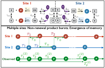
Figure 3: The sequence of turnovers for a pair of active sites that process substrates in parallel. The waiting times are denoted by $\tau$ and the forward recurrence times (see text) by $\tau_{+}$. The observed turnovers cannot distinguish which of the two active sites yielded the product and, hence, the turnover process is a pooling of the two independent turnover processes for each site. The generalization to more than two sites is obvious.

$$w_{\pi}(s|T_{p-1}^{(2)}) = w(s)[1-P(\tau_{+}<s|T_{p-1}^{(2)})]+$$ (23)

$$[1-\int_{0}^{s}w(s^{\prime})ds^{\prime}]w_{+}(s|T_{p-1}^{(2)})$$

In the above, the distribution of waiting times $w(s)$ is known from the analysis of the previous section and it only remains to determine the distribution $w_{+}(s|t)$ of the recurrence time. For a renewal process, the distribution of the forward recurrence time is related to the waiting time distribution and the enzymatic velocity by key-23 (23)

$$w_{+}(s|t)=w(t+s)+\int_{0}^{t}V(t-s^{\prime})w(s+s^{\prime})ds^{\prime}.$$ (24)

and this determines the waiting time distribution of the pooled process completely in terms of quantities that can be calculated from the component renewal processes.

How does the conditional dependence of the waiting time vary with the number of turnovers ? Since the entire conditional dependence derives from the distribution of the recurrence time, it is sufficient to examine its conditional dependence. For large times $t\gg T^{\star}$, it is known from both the deterministic and stochastic analysis that the enzymatic velocity becomes a constant, that is $\lim_{t\rightarrow\infty}V(t)=V_{ss}$. As a consequence, $\lim_{t\rightarrow\infty}w_{+}(s|t)=V_{ss}[1-W(s)]$ is independent of $t.$ In this limit, each site is in “equilibrium”, and the memory of the initial state of the process, which began with all sites free, is erased . Thus, the conditioning of the recurrence time of one site by the turnover time of another site, together with the deterministic initial condition, provides a mechanism for the statistical dependence between waiting times in the pooled process and of the emergence of molecular memory.

Extending this argument to $\nu$ binding sites, and denoting pooled quantities with the superscript $\nu$, it is clear that the waiting time $\tau_{p}^{(\nu)}$ for the $p$-th product is the shortest of a single waiting time and $\nu-1$ recurrence times conditioned on $t=T_{p-1}^{(\nu)}$ . Since $\tau_{p}^{(\nu)}$ being longer than $s$ implies both the waiting time and the $\nu-1$ recurrence times are longer than $s$, we have

$$P(\tau_{p}^{(\nu)}>s|T_{p-1}^{(\nu)})=P(\tau>s)[P(\tau_{+}>s|T_{p-1}^{(\nu)})]^{\nu-1}$$ (25)

where the factorizations on the right follow from independence and identity of the $\nu$ binding sites. Defining the waiting time distribution of the pooled process as $P(s<\tau_{p}^{(\nu)}<s+ds|T_{p-1}^{(\nu)})\equiv w_{\pi}(s|T_{p-1}^{(\nu)})ds$ and differentiating both sides of the above yields an explicit expression for $w_{\pi}(s|T_{p-1}^{(\nu)})$ in terms of the key single-site measures, the enzymatic velocity $V(t)$, the waiting time distribution $w(\tau)$, and the recurrence time distribution $w_{+}(s|t)$,

$$w_{\pi}(s|T_{p-1}^{(\nu)})=w(s)[1-P(\tau_{+}<s|T_{p-1}^{(\nu)})]^{\nu-1}+(\nu-1)[1-\int_{0}^{s}w(s^{\prime})ds^{\prime}][1-P(\tau_{+}<s|T_{p-1}^{(\nu)})]^{\nu-2}w_{+}(s|T_{p-1}^{(\nu)}).$$ (26)

.

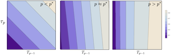
Figure 7: Heat maps depicting conditional dependence of $\tau_{p}$ on $T_{p-1}$ in the transient $p<p^{*}$ crossover $p\approx p^{*}$ and steady-state $p>p^{*}$ regimes for the MM mechanism.

In this expression, $\tau_{p}^{(\nu)}$ is conditionally dependent on $T_{p-1}^{(\nu)},$ and therefore on the previous waiting times $\tau_{1}^{(\nu)}\ldots\tau_{p-1}^{(\nu)}$, as long as $w_{+}(s|t)$ is dependent on $t$. Thus, the emergence of memory can now be traced explicitly to the transient in the enzymatic velocity, starting from the deterministic initial condition. Evaluating $w_{\pi}(s|T_{p-1}^{(\nu)})$ numerically for the MM mechanism for $T_{p-1}^{(\nu)}$ in the transient, crossover, and steady-state regimes quantitatively confirms this qualitative picture, Fig. (7) in the SI.

The waiting times become independent and identically distributed when the enzymatic velocity at each site reaches the steady state value. Then, inserting asymptotic form of the recurrence time distribution, we obtain $w_{\pi}^{(\nu)}(s)=-\frac{d}{ds}\left[P(\tau>s)\left\{V_{ss}\int_{s}^{\infty}P(\tau>s^{\prime})ds\right\}^{\nu-1}\right]$ giving the waiting time distribution in terms of survival probability and the steady-state enzymatic velocity at each site. This is the enzymatic analog of a well-known result in renewal theory key-36 (36).

V Statistical measures

In classical deterministic enzyme kinetics, the enzymatic velocity of $N$ independent and identical enzymes, $V(t)=d_{t}\langle n\rangle$, is a statistical measure of mean rate of product formation. The approach to steady-state is then marked by the asymptotic limit, $V_{ss}=\lim_{t\rightarrow\infty}V(t)$, in which the enzymatic velocity reaches its equilibrium value and becomes time independent. For $N\gg 1$, this asymptotic limit is realized at the onset of the reaction key-1 . This implies that the initial mean rate of product formation, i.e. the counting process alone, is sufficient to yield the steady-state enzymatic velocity $V_{ss}=\text{$\left.d_{t}\langle n\rangle\right|_{t\rightarrow 0}$}$ , and the transient regime remains unobserved key-17 .

In stochastic enzyme kinetics, in contrast, the statistical measures of counting and point processes for means and fluctuations, introduced in Section II, seem to provide an alternative description of product turnover kinetics in the number and time domain, respectively. It is pertinent to ask, then, how these seemingly unrelated statistical measures can be formally linked to demarcate the transient and steady-state regimes in enzyme kinetics at the molecular level, and how these results can be reconciled with the classical results of deterministic enzyme kinetics.

It is clear from the previous two sections that the turnover kinetics of single-enzyme networks is a renewal stochastic process with statistically independent waiting times, and thus no memory. For replica networks, there exist an initial transient regime with memory and a terminal steady-state without it. The switch from a non-renewal to renewal statistics in replica networks, with increasing turnover number, thus marks a crossover from transient to steady-state regime. In the steady-state, since waiting times are statistically independent and the governing statistics is renewal, below we use the results of the renewal theorems to formally link the statistical measures of counting and point processes key-23 (23, 37, 38).

In the steady state, statistical measures at each site are related to a pooled output, comprising of independent and identically distributed (iid) random variables. For counting process description, the iid random variables are the number of products formed at each site, resulting in a pooled output $n=n_{1}+n_{2}+\ldots n_{\nu}$ of $n$ total number of products formed at $\nu$ sites. From this, it follows that $V_{ss}^{(\nu)}=\nu V_{ss}$, where $V_{ss}=\lim_{t\rightarrow\infty}d_{t}\langle n_{i}\rangle$ with $i=1,2,\cdots\nu$. For point process description, the iid random variables are the waiting times $\tau_{p}^{(\nu)}$ between consecutive turnovers for $\nu$ sites, the sum of which $T_{p}^{(\nu)}=\tau_{1}^{(\nu)}+\ldots+\tau_{p}^{(\nu)}$ yields a pooled output for the $p$-th turnover time $T_{p}^{(\nu)}$. Since $\nu$ sites are independent and identically distributed, it follows that $\langle T_{p}^{(\nu)}\rangle=p\langle\tau^{(\nu)}\rangle$ and $\langle\tau^{(\nu)}\rangle=\frac{1}{\nu}\langle\tau\rangle$.

Further, the renewal theorem guarantees that the single-enzyme velocity asymptotes to the inverse mean waiting time, $\lim_{t\rightarrow\infty}V(t)=V_{ss}\equiv\langle\tau\rangle^{-1}$ key-23 (23) . This relates the statistical measures of means for counting and point processes, $V_{ss}^{(\nu)}\equiv\nu\langle\tau\rangle^{-1}$, for replica networks. From this it follows that the inverse mean waiting time $\langle\tau\rangle^{-1}$ in Eq. (18) can be identified as the single-enzyme velocity.

In the absence of temporal correlations between turnovers, the variance of the sum is the sum of variances, $\sigma_{T_{p}^{(\nu)}}^{2}=p\sigma_{\tau^{(\nu)}}^{2}$. The renewal theorem, then, dictates that the squared coefficient of variation, the randomness parameter, $r^{(\nu)}=\langle(\tau^{(\nu)}-\langle\tau^{(\nu)}\rangle)^{2}\rangle/\langle\tau^{(\nu)}\rangle^{2}$ asymptotes to the Fano factor $\rho_{ss}^{(\nu)}=\lim_{t\rightarrow\infty}\langle(n^{(\nu)}-\langle n^{(\nu)}\rangle)^{2}\rangle/\langle n^{(\nu)}\rangle$ for replica networks key-23 (23). A special case of this for $\nu=1$ was first introduced by Block, Schnitzer and coworkers key-24 (24) in the context of molecular motors, where it has widespread application key-39 (39, 40).

The above results show that for replica networks in the steady-state the description of turnovers in terms of counts, n, and waiting times, τ, are asymptotically equivalent as renewal theorems guarantee that $V_{ss}^{(\nu)}\equiv\nu\langle\tau\rangle^{-1}$ and $\rho_{ss}^{(\nu)}\equiv r^{(\nu)}$ key-23 (23, 37, 38). However, these results are not valid for replica networks in the transient regime where the governing statistics is non-renewal, $\langle T_{p}^{(\nu)}\rangle\neq p\langle\tau^{(\nu)}\rangle$, and depends on the turnover number $p$ through $T_{p}^{(\nu)}$. Moreover, the presence of correlations between waiting times clearly suggests that statistical measures in the transient regime should be redefined in terms of $T_{p}^{(\nu)}$, rather than $\tau_{p}^{(\nu)}$, as the former naturally contains correlations between waiting times. This motivates the following definitions for the turnover number dependent enzymatic velocity key-16 ,

$$V_{p}^{(\nu)}=\frac{p}{\langle T_{p}^{(\nu)}\rangle}$$ (27)

and the randomness parameter associated with $T_{p}^{(\nu)}$

$$r_{p}^{(\nu)} =p\frac{\langle(T_{p}^{(\nu)}-\langle T_{p}^{(\nu)}\rangle)^{2}\rangle}{\langle T_{p}^{(\nu)}\rangle^{2}}$$

$$=p\frac{{\sum_{i}^{p}\langle(\delta\tau_{i}^{(\nu)})^{2}\rangle+\sum_{i\neq j}^{p}\langle\delta\tau_{i}^{(\nu)}\delta\tau_{j}^{(\nu)}\rangle}}{\langle\sum_{i}^{p}\tau_{i}^{(\nu)}\rangle^{2}},$$ (28)

where $\delta\tau_{i}=\tau_{i}-\left<\tau_{i}\right>$.

The turnover number dependent enzymatic velocity $V_{p}^{(\nu)}$ and randomness parameter $r_{p}^{(\nu)}$ provide new statistical measures of means and fluctuations for replica networks that can be used both in transient and steady-state regimes, simply by increasing $p$. In Eq. (27), the crossover from non-renewal $\langle T_{p}^{(\nu)}\rangle\neq p\langle\tau^{(\nu)}\rangle$ to renewal $\langle T_{p}^{(\nu)}\rangle=p\langle\tau^{(\nu)}\rangle=\frac{p}{\nu}\langle\tau\rangle$ statistics with increasing $p$, guarantees that the steady-state enzymatic velocity is asymptotically recovered, $\lim_{p\rightarrow\infty}V_{p}^{(\nu)}=\nu\langle\tau\rangle^{-1}\equiv V_{ss}^{(\nu)}$. In Eq. (28), similarly, the increase in $p$ brings about a switch from non-renewal statistics with statistically dependent waiting times $\sum_{i\neq j}^{p}\langle\delta\tau_{i}^{(\nu)}\delta\tau_{j}^{(\nu)}\rangle\neq 0$ to renewal statistics with statistically independent waiting times, $\sum_{i\neq j}^{p}\langle\delta\tau_{i}^{(\nu)}\delta\tau_{j}^{(\nu)}\rangle=0$. In the asymptotic limit of large $p$, thus, $r_{p}^{(\nu)}$ reduces to the steady-state definition, $r^{(\nu)}=\langle(\delta\tau^{(\nu)})^{2}\rangle/\langle\tau^{(\nu)}\rangle^{2}$, which is equivalent to the steady-state Fano factor $\rho_{ss}^{(\nu)}$, as expected from the renewal theorem key-23 (23).

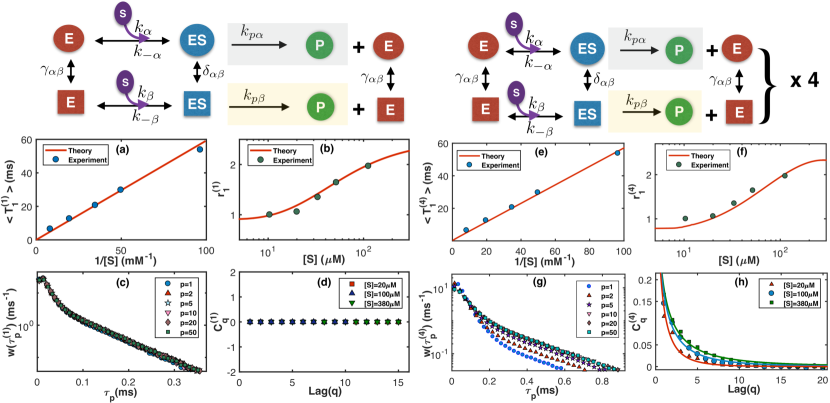
Figure 4: Quantitative comparison of turnover statistics for single- and quadruple-site ppMM models. Rate constants are estimated by simultaneously fitting analytical expressions for $\langle T_{1}^{(\nu)}\rangle$ and $r_{1}^{(\nu)}$ to experimental data. Exact numerical sampling with these parameters is used to generate distributions $w(\tau_{p})$ and compute correlations $C_{q}$. The renewal character of the single-site model and its lack of memory is confirmed in panels (c) and (d). Points are simulation data using best-fit rate parameters and solid lines are stretched-exponential fits $C_{q}^{(4)}=\exp[-(q/q_{0})^{\beta}]$ with $q_{0}=0.25$, $\beta=0.47,0.42,0.39$ for $[S]=20\mu\mbox{M},100\mu M,380\mu M$, respectively.

Eqs. (27) and (28) are the key results of this work as they provide the statistical measures of point process for single-enzyme and replica networks in transient and steady-state regimes. Their link to counting process, as shown above, relies on the change of statistics from non-renewal at lower $p$ to renewal at higher $p$. This naturally introduces a critical turnover number $p^{*}$ which demarcates the transient $p\ll p^{*}$ from steady-state $p\gg p^{*}$ regime. In the steady-state, $V_{p}^{(\nu)}$asymptotes to

$$V_{p\gg p^{*}}^{(\nu)}=\nu\langle\tau\rangle^{-1}\equiv V_{ss}^{(\nu)},$$ (29)

Similarly, $r_{p}^{(\nu)}$in the steady-state asymptotes to

$$r_{p\gg p^{*}}^{(\nu)}=r^{(\nu)}\equiv\rho_{ss}^{(\nu)}.$$ (30)

In the transient regime, $p\ll p^{*}$, both these equivalences are necessarily violated as the governing statistics is non-renewal.

Eqs. (29) and (30), while subsuming the results of renewal theorems in the steady-state, provide an empirical test of non-stationarity in experimental data and a diagnostic for the emergence of memory in the transient regime. In the next section, we show how these equalities can be used to determine $p^{*}$.

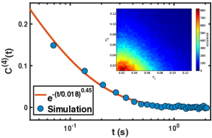
Figure 5: Normalized correlation $C^{(4)}(t)$ for quadruple-site PPMM mechanism at $[S]=100\mu M$. Points are simulation data and the solid line is a stretched exponential $e^{-(t/t_{0})^{\beta}}$ with $t_{0}=0.018$s and $\beta=0.45$. The inset is the joint probability $w(\tau_{1}^{(4)},\tau_{2}^{(4)})$ of consecutive waiting times, which shows that a short (long) first waiting time is more likely to be followed by a short (long) second waiting time, in agreement with experiment.

VI Comparison with data

We now apply the theory developed in the preceding sections to analyze the data from the landmark experiment in which molecular memory was first observed key-12 . In this experiment, the catalysis of non-fluorescent substrates to fluorescent products by the tetrameric enzyme $\beta$-galactosidase over a range of substrate concentrations was monitored using fluorescence spectroscopy. Waiting times were obtained from the primary data of product turnovers as discrete fluorescence bursts, and the distribution $w(\tau)$ and its first two moments were computed for each substrate concentration. While the variation of mean waiting time with $1/[S]$ was linear at low substrate concentrations, the monotonic increase in the randomness parameter with $[S]$, bounded below by one, was a signature of dynamic disorder. The joint distribution, $w(\tau_{p},\tau_{p+q})$ of the waiting times, $q$ turnovers apart, revealed that turnover events were not statistically independent but that a short (or long) first waiting time was more likely to be followed by another short (or long) second waiting time. This was a signature of positive molecular memory. The correlation of waiting times, $C_{q}=\langle\delta\tau_{p}\delta\tau_{p+q}\rangle$, remained appreciable and, when expressed in terms of a scaled time $t=q\left<\tau\right>$, could be collapsed to a single stretched-exponential $C(t)=\exp[-(t/t_{0})^{\beta}]$ with $\beta=0.45$ and $t_{0}=0.018$s.

Experimental results reveal statistically dependent waiting times and dynamic disorder in enzyme turnover kinetics of $\beta$-galactosidase. Following the analysis of Sections III and IV, this motivates us to select the ppMM network with four replicas as the minimal model to understand the kinetics. For comparison, we also consider a hypothetical single-enzyme ppMM network, with identical parameters, but only a single binding site. We use the results of Section III and the SI to compute the marginal distribution $w(T_{1}^{(\nu)})$, where superscript to $T_{p}^{(\nu)}$ denotes the results for a single site $(\nu=1)$ and quadruple sites $(\nu=4).$ From $w(T_{1}^{(\nu)})$ thus obtained, we analytically compute the mean first turnover time, $\langle T_{1}^{(\nu)}\rangle$, and the randomness parameter, $r_{1}^{(\nu)}$, as function of the 8 rates constants. A simultaneous least-squares fit to the experimental data provides us with the maximum-likelihood parameters of each model. These are listed in Table 3 of the SI and the corresponding fits are shown in the top four panels of Fig. (4).

The excellent agreement between model and data for both single- and quadruple-site models leaves little to distinguish between them. Since both models have the same number of parameters, and hence equal model complexity, they appear to be equally plausible models for data derived from the marginal distribution. This degeneracy in model space is lifted by using data from the joint distribution, as we now show.

Mechanism	Sites	Memory	Correlations	$r_{1}^{(\nu)}$vs $[S]$
MM	1	Absent	$C_{q}^{(1)}=0$	$r_{1}^{(1)}\leq 1$
ppMM	1	Absent	$C_{q}^{(1)}=0$	$r_{1}^{(1)}\geq 1$
MM	4	Anti-correlated	$C_{q}^{(4)}\leq 0$	$r_{1}^{(4)}\leq 1$
ppMM	4	Correlated	$C_{q}^{(4)}\geq 0$	$r_{1}^{(4)}\geq 1$
$\beta$-galactosidase	4	Correlated	$C_{q}\geq 0$	$r\geq 1$

Table 2: Qualitative comparison of turnover statistics for MM and ppMM models for single and multiple binding sites. The ppMM model, with conformational fluctuations and four binding sites, best agrees with the experimentally obtained turnovers of $\beta$-galactosidase.

Since we have not found a way to obtain the joint distributions of the Markov chain analytically, we compute them numerically from a time series of turnovers, sampled using the Doob-Gillespie algorithm key-41 (41) with chain parameters set to the above least-squares estimates. The distribution of $\tau_{p}^{(\nu)}$ and the correlation function $C_{q}^{(\nu)}$ are shown in the bottom four panels of Fig.(4).

There is, now, a clear distinction between single-site and quadruple-site models. The first distinction appears in the distribution of waiting times $\tau_{p}.$ These are identically and independently distributed for the single-site model (panels (c) and (d)) but neither identically nor independently distributed for the quadruple-site model (panels (g) and (h)). This confirms the results of Sections III and IV that a model with fermionic hidden states can only yield a renewal process and that multiple binding sites are necessary for molecular memory. Focussing on panel (h), the normalized correlation function has an excellent fit to a stretched exponential function $C_{q}^{(4)}=\exp[-(q/q_{0})^{\beta}]$ with parameters $q_{0}=0.25$ and $\beta=0.47,0.42,0.39$ for the substrate concentrations $[S]=20\mu\mbox{M},100\mu M,380\mu M$ reported in the experiment. Continuing in Fig. (5) we plot the normalized correlation function $C^{(4)}(t)$ in scaled time $t=\langle\tau_{1}^{(4)}\rangle q$ following experiment. There is a quantitative match between experiment and theory, with both following a stretched exponential function $C^{(4)}(t)=\exp[-(t/t_{0})^{\beta}]$ with $t_{0}=0.018$s and $\beta=0.45$ for $[S]=100\mu$M. In addition, the pseudocolor plot of the joint distribution of the first and second waiting times, $w(\tau_{1}^{(4)},\tau_{2}^{(4)})$, shows that a short (or long) first waiting time is more likely to be followed by a short (or long) second waiting time (inset) in agreement with the molecular memory observed in experiment.

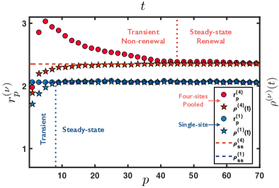
Figure 6: Randomness parameters and Fano factors for the ppMM obtained from numerically computed trajectories of the single- and quadruple-site models. For quadruple-site model, these measures of counting and point processes are asymptotically equivalent in the (renewal) steady state but differ in the (non-renewal) transient state, in agreement with Eq. (30). Memory persists as long as equality is violated. For memoryless single-site model, the duration of the transient is determined by the the counting process description, i.e. the time required for the Fano factor to reach its steady-state value. Parameter values are listed in Table 3 of the SI

For comparison, we repeat the above calculations for the MM model and summarize our findings in Table 2. The heat map of the joint distribution of successive waiting times, $w(\tau_{1},\tau_{2})$, shows negative correlations for the MM model, but positive correlations for the ppMM model. In the stationary state, the randomness parameter is negative for the MM model, but positive for the ppMM model. Only the ppMM model, containing both multiple binding sites and conformational fluctuations, is in agreement with experiment, as summarized in the last two rows of the table. While multiple sites alone yield memory, conformational fluctuations are necessary for the correct sign of the correlation function and the correct magnitude of the randomness parameter.

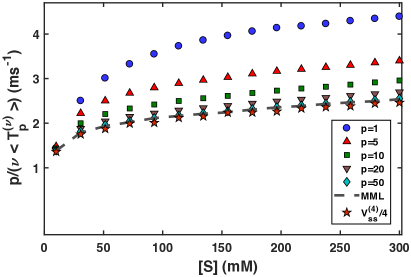
Figure 8: The variation with substrate concentration, $[S]$, of the stochastically defined enzymatic velocity, $V_{p}^{(\nu)}=p/\langle T_{p}^{(\nu)}\rangle$, for product turnovers $p=1,5,10,20,50$, for the quadruple-site model. The enzymatic velocity converges to its steady-state value with the increase in $p$. This steady-state value is $\nu\langle\tau\rangle^{-1}$, where $\langle\tau\rangle^{-1}$ is the single-enzyme velocity $v_{1}^{(1)}$, given by the Michaelis-Menten-like (MML) equation, Eq. (38) , shown as the dashed line. These agree with the classical definition of the steady-state enzymatic velocity $V_{ss}^{(4)}$ plotted with $\star$. Parameter values are listed in Table .3

We now use Eqs. (29) and (30) of Section V to determine $p^{*}$, and thus demarcate the transient $p\ll p^{*}$ and steady-state $p\gg p^{*}$ regimes for the ppMM model. The variation of $V_{p}^{(\nu)}$ with substrate concentration is shown in Fig. (8) of the SI. The enzymatic velocity in the transient regime, $V_{p\ll p^{*}}^{(\nu)}$, deviates from the steady-state value $\nu\langle\tau\rangle^{-1}$ , where $\langle\tau\rangle^{-1}$ is the Michaelis-Menten-like (MML) equation, Eq. (38) in the SI. In the steady-state, $V_{p\gg p^{*}}^{(\nu)}$ asymptotically approaches both the single-enzyme MML equation and the classical steady-state enzymatic velocity $V_{ss}^{(\nu)}$, in agreement with Eq. (29). Similar analysis for the statistical measures of fluctuations is presented in Fig. (6) , which shows the variation of $r_{p}^{(\nu)}$ with $p$ and $\rho^{(\nu)}(t)$ with $t$ for $\nu=1,4$. The comparison shows that the equivalence between the randomness parameter and the steady-state Fano factor is violated in the transient regime, $r_{p\ll p^{*}}^{(\nu)}\neq\rho_{ss}^{(\nu)}$, but is asymptotically recovered in the steady-state regime $p\gg p^{*}$, in agreement with Eq. (30).

The fading of memory, the convergence of the waiting time distributions, and the equality of the statistical measures all occur at roughly $p^{\star}\approx 50$ turnovers in this model.

VII Conclusion and Future work

The stochastic time-domain approach presented here, when used in combination with the stochastic number-domain approach, namely CME, provides the most detailed information of enzymatic reactions and can be used to extract mechanistic information that is lost in classical deterministic theories of enzyme kinetics.

Our work shows that the mechanism for the emergence of molecular memory will always be operative through the transient phase in an enzyme with multiple binding sites. It can thus be viewed as a null model (in the sense of a null hypothesis) and should be tested against before embarking on a search for more elaborate models of molecular memory that may require, for instance, interactions between binding sites.

Deviation from hyperbolicity in stochastic enzymatic networks emerges from the concerted action of independent, and hence non-interacting, multiple binding sites. This form of “cooperativity” is dynamic in nature key-42 (42), which arises from temporal correlations between enzymatic turnovers in the transient regime, and vanishes in the steady state regime. This contrasts the traditional description of enzyme cooperativity in equilibrium, in which multiplicity of binding sites and interactions between them are inextricably linked key-1 . The replica approach presented here can be extended to include interactions between binding sites. This can, then, pave a way to understand the combined effect of stochasticity and interaction in generating molecular cooperativity in the steady-state.

Our study extends beyond the simple homogeneous mechanisms studied here, to more complex mechanisms including inhibitors key-14 ; key-43 (43, 44) and to heterogenous catalysis of, for example, nano-particle clusters containing numerous binding sites key-45 (45). In the latter case, the method presented here can be used to estimate the catalytic rate from turnover time data through a new kinetic measure, the heterogeneity index, that can quantify fluctuations from non-identical binding sites key-57 (18, 19, 20). In addition, the analysis can be extended to unravel hidden intermediate states key-46 (46, 47).

In the context of molecular motors, the renewal theorems have been known to link the mean and variance of the physical distance moved by the motor with the corresponding mean and variance of the number of products formed under stationary condition key-25 (25, 26). Both are linearly proportional to time, with proportionality constants being enzymatic velocity for the measure of mean, and diffusion coefficient for the measure of variance. The relations between the statistical measures of counting and point process, for the mean and variance, presented here, and their dependence on the turnover number, can be used to generalize the corresponding expressions for molecular motors to non-stationary conditions, where transport coefficients are expected to be turnover number dependent.

Fluctuation statistics of mesoscopic quantum transport in nanoscale devices analyzed in terms of fixed time (counting process) or fluctuating time (point process) description using a master equation framework key-48 (48, 49). While the renewal theorems provide formal relations between counting and point process statistics, the violation of renewal statistics and the analysis of non-renewal fluctuation statistics, in which temporal correlations between discrete quantum events are accounted for, is a relatively new premise key-50 (50, 51). The generality of our results, for both renewal and non-renewal fluctuation statistics, can provide impetus to explore a transient phase in mesoscopic quantum transport.

The sensitivity of the waiting time distributions to the reaction mechanism, both in the transient and steady states, invites the application of Bayesian probability to calculate the posterior probability $P(\mathcal{M}|\{\tau_{p}\})$, of a model $\mathcal{M}$ given waiting time data $\{\tau_{p}\}$ and, thereon, to machine learning reaction mechanisms from turnover data key-52 (52, 53, 54).

To conclude, our work shows that complex forms of molecular memory can arise from the combined action of simple memoryless steps, provides a theoretical framework within which such action can be studied systematically, and suggests experiments to test the validity of this generic mechanism.

Supplementary Material

See the supplementary information (SI) for detailed solution of the chemical master equations for single-site and multiple-sites catalysis.

Data Availability

The data that supports the findings are available within the article, in supplemental material and in reference number [9].

Supplementary Information

I. Single-Site catalysis as a renewal process

Section III in the main text has established that the turnovers for single-site stochastic networks form renewal processes, that is, the waiting time distributions are identically and independently distributed. The latter has been used to show how the waiting time distribution can be calculated from the CME describing the single-site Michaelis-Menten (MM) network. The purpose of this section is to provide explicit results for the waiting time distribution $w(T_{1}^{(1)})$ for the single-site parallel pathway Michaelis-Menten (ppMM) network, from which the mean waiting time and randomness parameter can be computed.

VII.1 Turnover statistics of single-enzyme ppMM network

For the parallel-pathway Michaelis-Menten model, the states are $\boldsymbol{n}=(\boldsymbol{n}^{\star},n)$, with $\boldsymbol{n}^{\star}=(n_{E_{\alpha}},n_{ES_{\alpha}},n_{E_{\beta}},n_{ES_{\beta}})$ and the mass conservation constraint $n_{E_{\alpha}}+n_{E_{\beta}}+n_{ES_{\alpha}}+n_{ES_{\beta}}=1$. This implies that state of the reaction at any time $t$ is of the form $(1,0,0,0,n)$ or $(0,1,0,0,n)$ or $(0,0,1,0,n)$ or $(0,0,0,1,n)$. Labeling these as $(E_{\alpha},n)$, $(ES_{\alpha},n)$, $(E_{\beta},n)$ and $(ES_{\beta},n)$ respectively the CME can be written as

$$\partial_{t}P(E_{\alpha},n) =k_{-\alpha}P(ES_{\alpha},n)+\gamma_{\alpha\beta}P(E_{\beta},n)-(k_{\alpha}^{\prime}+\gamma_{\alpha\beta})P(E_{\alpha},n)+k_{p\alpha}P(ES_{\alpha},n-1)$$

$$\partial_{t}P(E_{\beta},n) =k_{-\beta}P(ES_{\beta},n)+\gamma_{\alpha\beta}P(E_{\alpha},n)-(k_{\beta}^{\prime}+\gamma_{\alpha\beta})P(E_{\beta},n)+k_{p\beta}P(ES_{\beta},n-1)$$

$$\partial_{t}P(ES_{\alpha},n) =k_{\alpha}^{\prime}P(E_{\alpha},n)+\delta_{\alpha\beta}P(ES_{\beta},n)-(k_{-\alpha}+\delta_{\alpha\beta}+k_{p\alpha})P(ES_{\alpha},n)$$

$$\partial_{t}P(ES_{\beta},n) =k_{\beta}^{\prime}P(E_{\beta},n)+\delta_{\alpha\beta}P(ES_{\alpha},n)-(k_{-\beta}+\delta_{\alpha\beta}+k_{p\beta})P(ES_{\beta},n)$$ (31)

The analysis of Section III in the main text shows that the marginal distribution can be written as a sum over the hidden states $\boldsymbol{n}^{\star}$. For the ppMM network, thus, $P(n)=P(E_{\alpha},n)+P(E_{\beta},n)+P(ES_{\alpha},n)+P(ES_{\beta},n)$, and the cumulative distribution of the turnover time is

$$P(T_{p}\leq t)=\sum_{n=p}^{\infty}P(E_{\alpha},n)+P(E_{\beta},n)+P(ES_{\alpha},n)+P(ES_{\beta},n)$$ (32)

and waiting time distribution is

$$w(s)=-\left[\partial_{t}P(E_{\alpha},p-1)+\partial_{t}P(E_{\beta},p-1)+\partial_{t}P(ES_{\alpha},p-1)+\partial_{t}P(ES_{\beta},p-1)\right]_{t=s}$$ (33)

The system of differential equations must be solved with the initial condition that, at $t=T_{p-1},$ the reaction has just entered the state $(E_{\alpha},p-1)$ or $(E_{\beta},p-1)$. The appropriate initial condition is $P(\boldsymbol{n})=\theta\delta_{\boldsymbol{n}\boldsymbol{m}_{1}}+(1-\theta)\delta_{\boldsymbol{n}\boldsymbol{m}_{2}}$ with $\boldsymbol{m}_{1}=(E_{\alpha},p-1)$, $\boldsymbol{m}_{2}=(E_{\beta},p-1)$ and $0\leq\theta\leq 1$. This gives an identical $4\times 4$ system of differential equations for the waiting times and repeating the previous argument shows that $\tau_{p}$ are identically and independently distributed.

Using the notation $\boldsymbol{P}(t)=[P(E_{\alpha}),P(ES_{\alpha}),P(E_{\beta}),P(ES_{\beta})]$ and with the irrelevant index $p$ suppressed, the $4\times 4$ system of equations determining the waiting time distribution can be written as $\partial_{t}$$\boldsymbol{P}(t)=\boldsymbol{A}\cdot\boldsymbol{P}(t)$ where

$$\boldsymbol{A}=\begin{bmatrix}-(k_{\alpha}^{\prime}+\gamma_{\alpha\beta})&k_{-\alpha}&\gamma_{\alpha\beta}&0\\ k_{\alpha}^{\prime}&-(k_{-\alpha}+\delta_{\alpha\beta}+k_{p\alpha})&0&\delta_{\alpha\beta}\\ \gamma_{\alpha\beta}&0&-(k_{\beta}^{\prime}+\gamma_{\alpha\beta})&k_{-\beta}\\ 0&\delta_{\alpha\beta}&k_{\beta}^{\prime}&(k_{-\beta}+\delta_{\alpha\beta}+k_{p\beta})\end{bmatrix}$$ (34)

The matrix exponential can be computed using the spectral representation $\boldsymbol{A}=\text{$\boldsymbol{V\Lambda V}$}^{-1}$ where $\boldsymbol{V}$ is the matrix of eigenvectors of $\boldsymbol{A}$ and $\boldsymbol{\Lambda}$ is diagonal matrix of its eigenvalues. A tedious calculation then yields

$$w(s)=\frac{{1}}{(A-B)(C-D)}\left[\frac{(C-D)\eta_{A}e^{-As}}{(A-C)(A-D)}-\frac{(C-D)\eta_{B}e^{-Bs}}{(B-C)(B-D)}+\frac{(A-B)\eta_{C}e^{-Cs}}{(C-A)(C-B)}-\frac{(A-B)\eta_{D}e^{-Ds}}{(D-A)(D-B)}\right]$$ (35)

where where $\eta_{I}={I(k_{p\alpha}A_{1}+k_{p\beta}A_{2})-(k_{p\alpha}B_{1}+k_{p\beta}B_{2})-I^{2}k_{p\alpha}k_{\alpha}[S]}$ with $I=A,B,C,D$. In the above equation, $A$, $B$, $C$ and $D$ are the effective rate constants which are the solutions of the quartic equation $z^{4}+\lambda_{1}z^{3}+\lambda_{2}z^{2}+\lambda_{3}z+\lambda_{4}=0$ and $A_{1}$, $A_{2}$, $B_{1}$, $B_{2}$, $\lambda_{1}$, $\lambda_{2}$, $\lambda_{3}$ and $\lambda_{4}$, have involved dependences on the rate constants of the ppMM model. They are given by

$${A_{1}} = k_{\alpha}k_{\beta}[S]^{2}+k_{\alpha}(k_{-\beta}+k_{p\beta}+{\gamma_{\alpha\beta}}+{\delta_{\alpha\beta}})[S]$$

$${B_{1}} = k_{\alpha}k_{\beta}(k_{p\beta}+{\delta_{\alpha\beta}})[S]^{2}+(k_{\alpha}{\gamma_{\alpha\beta}}(k_{-\beta}+k_{p\beta}+{\delta_{\alpha\beta}})+{\gamma_{\alpha\beta}}{\delta_{\alpha\beta}}k_{\beta})[S]$$

$${A_{2}} = (k_{\alpha}{\delta_{\alpha\beta}}+k_{\beta}{\gamma_{\alpha\beta}})[S]$$

$${B_{2}} = k_{\alpha}k_{\beta}{\delta_{\alpha\beta}}[S]^{2}+(k_{\beta}{\gamma_{\alpha\beta}}(k_{-\alpha}+k_{p\alpha}+{\delta_{\alpha\beta}})+{\gamma_{\alpha\beta}}{\delta_{\alpha\beta}}k_{\alpha})[S]$$

$${\lambda_{1}} = (k_{\alpha}+k_{\beta})[S]+k_{-\alpha}+k_{-\beta}+k_{p\alpha}+k_{p\beta}+2({\gamma_{\alpha\beta}}+{\delta_{\alpha\beta}})$$

$${\lambda_{2}} = k_{\alpha}k_{\beta}[S]^{2}+[(k_{\alpha}k_{-\beta}+k_{\beta}k_{-\alpha})+(k_{p\alpha}+k_{p\beta}+\gamma_{\alpha\beta}+2{\delta_{\alpha\beta}})(k_{\alpha}+k_{\beta})][S]$$

$$+(k_{-\alpha}k_{-\beta}+k_{-\alpha}k_{p\beta}+k_{-\beta}k_{p\alpha}+k_{p\alpha}k_{p\beta})$$

$$+(2\gamma_{\alpha\beta}+\delta_{\alpha\beta})(k_{-\alpha}+k_{p\alpha}+k_{-\beta}+k_{p\beta})+4\gamma_{\alpha\beta}\delta_{\alpha\beta}$$

$${\lambda_{3}} = k_{\alpha}k_{\beta}(k_{p\alpha}+k_{p\beta}+2\delta_{\alpha\beta})[S]^{2}+(k_{\alpha}[k_{p\alpha}k_{-\beta}+k_{p\alpha}k_{p\beta}+(\gamma_{\alpha\beta}+\delta_{\alpha\beta})(k_{p\alpha}$$

$$+k_{p\beta}+k_{-\beta})+2{\gamma_{\alpha\beta}}{\delta_{\alpha\beta}}]+k_{\beta}[k_{p\beta}k_{-\alpha}+k_{p\alpha}k_{p\beta}+(\gamma_{\alpha\beta}+\delta_{\alpha\beta})(k_{p\alpha}$$

$$+k_{p\beta}+k_{-\alpha})+2{\gamma_{\alpha\beta}}{\delta_{\alpha\beta}}])[S]+2\gamma_{\alpha\beta}(k_{-\alpha}k_{-\beta}+k_{-\alpha}k_{p\beta}+k_{-\beta}k_{p\alpha}+k_{p\alpha}k_{p\beta}$$

$$+\delta_{\alpha\beta}(k_{-\alpha}+k_{-\beta}+k_{p\alpha}+k_{p\beta}))$$

$${\lambda_{4}} = k_{\alpha}k_{\beta}(k_{p\alpha}k_{p\beta}+\delta_{\alpha\beta}(k_{p\alpha}+k_{p\beta}))[S]^{2}+\gamma_{\alpha\beta}(k_{-\alpha}k_{\beta}k_{p\beta}+k_{-\beta}k_{\alpha}k_{p\alpha}$$

$$+k_{p\alpha}k_{p\beta}(k_{\alpha}+k_{\beta})+\delta_{\alpha\beta}(k_{\alpha}+k_{\beta})(k_{p\alpha}+k_{p\beta}))[S]$$

Now $w\{s)=\mathcal{L}w(\tau)=\int_{0}^{\infty}d\tau e^{-is\tau}w(\tau)$, where $\mathcal{L}$ is the Laplace transform operator. By corollary,

$$w(T_{1}^{(1)})\equiv w(\tau)=\mathcal{L}^{-1}w(s),$$ (36)

the explicit form for which is unwieldy and not presented here. It can be obtained numerically from the roots of the quartic equation, expressed above. However, the moments of $w(\tau)$ defined as $\langle\tau^{n}\rangle=\int_{0}^{\infty}d\tau\tau^{n}w(\tau)$ can be directly obtained from Eq. (35) using the identity $\langle\tau^{n+1}\rangle=(-1)^{n+1}\frac{{d^{n+1}w(s)}}{ds^{n+1}}$. The mean waiting time, $\langle\tau\rangle=-\frac{dw(s)}{ds}$, thus simplifies to

$$\langle T_{1}^{(1)}\rangle\equiv\langle\tau\rangle = \frac{\lambda_{3}-k_{21}A_{1}-k_{22}A_{2}}{\lambda_{4}}$$ (37)

$$= \frac{E[S]^{2}+F[S]+G}{H[S]^{2}+I[S]},$$

the reciprocal of which yields the Michaelis-Menten-like (MML) equation for the enzymatic velocity

$$v_{1}^{(1)}=\langle\tau\rangle^{-1}=\frac{H[S]^{2}+I[S]}{E[S]^{2}+F[S]+G},$$ (38)

where

$$E = k_{\alpha}k_{\beta}(k_{p\beta}+2\delta_{\alpha\beta})$$

$$F = k_{\beta}k_{-\alpha}k_{p\beta}+(\gamma_{\alpha\beta}+\delta_{\alpha\beta})(k_{\beta}k_{-\alpha}+k_{\alpha}k_{-\beta}+k_{\beta}k_{p\alpha}+(k_{\alpha}+k_{\beta})(k_{p\beta}+2{\gamma_{\alpha\beta}}\delta_{\alpha\beta})$$

$$G = 2{\gamma_{\alpha\beta}}(k_{-\alpha}k_{-\beta}+k_{-\alpha}k_{p\beta}+k_{-\beta}k_{p\alpha}+k_{p\alpha}k_{p\beta}+\delta_{\alpha\beta}(k_{-\alpha}+k_{-\beta}+k_{p\alpha}+k_{p\beta}))$$

$$H = k_{\alpha}k_{\beta}(k_{p\alpha}k_{p\beta}+\delta_{\alpha\beta}(k_{p\alpha}+k_{p\beta})$$

$$I = {\gamma_{\alpha\beta}}(k_{\alpha}(k_{p\alpha}k_{-\beta}+k_{p\alpha}k_{p\beta})+k_{\beta}(k_{-\alpha}k_{p\beta}+k_{p\alpha}k_{p\beta})+{\delta_{\alpha\beta}}(k_{p\alpha}+k_{p\beta})(k_{\alpha}+k_{\beta}))$$

The randomness parameter, $r_{1}^{(1)}$, can similarly be computed from the first and second moments of $w(T_{1}^{(1)})$.

II. Multiple-site catalysis as a non-renewal process

The waiting time distribution for multiple-site catalysis is non-renewal and depends on the turnover number $p$. Hence, the analysis of the preceding section cannot be used to obtain $w(T_{p}^{(\nu)})$. The method of Cox and Smith, based on the superposition of renewal processes, provides a simple way to obtain $w(T_{1}^{(\nu)})$ for multiple sites from the waiting time distribution of a single site key-36 (36). In this method, the waiting time distribution for the pooled process, i.e. the first product turnover for catalysis at $\nu$ independent and identical sites, can be expressed as

$$w(T_{1}^{(\nu)})=\nu\leavevmode\nobreak\ w(\tau)\left(\int_{\tau}^{\infty}\leavevmode\nobreak\ w(t)\leavevmode\nobreak\ dt\right)^{\nu-1}$$ (39)

where $w(\tau)=w(T_{1}^{(1)})$ is given by Eq. (36). For the ppMM network, we use Eq. (35) to compute $w(T_{1}^{(\nu)})$, and thus obtain $\langle T_{1}^{(\nu)}\rangle$ and $r_{1}^{(\nu)}$ .

Model	Sites	$k_{\alpha}$ ($M^{-1}s^{-1}$)	$k_{-\alpha}$ ($s^{-1})$	$k_{\beta}$ ($M^{-1}s^{-1}$)	$k_{-\beta}$ ($s^{-1})$	$k_{p\alpha}$ ($s^{-1})$	$k_{p\beta}$ ($s^{-1})$	$\gamma_{\alpha\beta}$ ($s^{-1})$	$\delta_{\alpha\beta}$ ($s^{-1})$
ppMM	1	$2.2\times 10^{6}$	$6.0$	$2.2\times 10^{6}$	$6.0$	$60.3$	$2.9$	$7.5$	$16.0$
ppMM	4	$5.6\times 10^{5}$	$0.4$	$5.0\times 10^{5}$	$0.4$	$14.6$	$0.01$	$1.6\times 10^{2}$	$1.05$

Table 3: Model parameters estimated from a simultaneous least-squares fit of $\langle T_{1}^{(\nu)}\rangle$ and $r_{1}^{(\nu)}$ to experimental data key-12 .

To compute the $p$-th dependent marginal and joint distributions of turnover and waiting times, we carry out stochastic simulations. We sample $10^{6}$ stochastic trajectories of the Markov chain for MM and ppMM networks, using the Doob-Gillespie algorithm key-41 (41), and obtain a time series of turnover times $T_{p}^{(\nu)}$ and waiting times $\tau_{p}^{(\nu)}$. We normalize histograms of these quantities to obtain the marginal distributions $w(T_{p}^{(\nu)})$ and $w(\tau_{p}^{(\nu)})$ and their summary statistics. The trajectories are also used to compute the number of products $n^{(\nu)}$ formed at time $t$ and their distribution $w(n^{(\nu)},t)$. The mean and variance of the number distribution yield the mean number of products formed $\left<n^{(\nu)}(t)\right>$ in time $t$, its rate of change $\frac{d\langle n^{(\nu)}(t)\rangle}{dt}=\lim_{\Delta t\rightarrow 0}\frac{\langle n^{(\nu)}(t+\Delta t)\rangle-\langle n^{(\nu)}(t)\rangle}{\Delta t}$, and the Fano factor $\rho^{(\nu)}(t)=\frac{\langle(n^{(\nu)}(t)-\langle n^{(\nu)}(t)\rangle)^{2}\rangle}{\langle n^{(\nu)(}(t)\rangle}$. The joint distribution of the $p$-th and $(p+q)$-th waiting times, $w(\tau_{p}^{(\nu)},\tau_{p+q}^{(\nu)})$ is similarly calculated from the ensemble of trajectories. The latter is used to obtain the normalized waiting time correlations, $C_{q}^{(\nu)}=\frac{\left<\delta\tau_{p}^{(\nu)}\delta\tau_{p+q}^{(\nu)}\right>}{\sqrt{\langle\tau_{p}^{(\nu)}\tau_{p}^{(\nu)}\rangle}\sqrt{\langle\tau_{p+q}^{(\nu)}\tau_{p+q}^{(\nu)}\rangle}}$ , where $p,q=1,2,3,\cdots$.

References

- (1) A. Cornish-Bowden and A. Cornish-Bowden, Fundamentals of enzyme kinetics, Vol. 510 (Wiley-Blackwell Weinheim, Germany, 2012).
- (2) L.Michaelis and M.L.Menten, Biochem.Z. 49, 333 (1913).
- (3) A. Cornish-Bowden, Perspectives in Science 4, 3 (2015).
- (4) U. Deichmann, S. Schuster, J.-P. Mazat, and A. Cornish- Bowden, The FEBS journal 281, 435 (2014).
- (5) H. Lineweaver and D. Burk, Journal of the American chemical society 56, 658 (1934).
- (6) F. Wong, A. Dutta, D. Chowdhury, and J. Gunawardena, Proceedings of the National Academy of Sciences 115, 9738 (2018).
- (7) H. P. Lu, L. Xun, and X. S. Xie, Science 282, 1877 (1998).
- (8) X. Xie and H. Lu, in Single Molecule Spectroscopy (Springer, 2001) pp. 227–240.
- (9) B. P. English, W. Min, A. M. Van Oijen, K. T. Lee, G. Luo, H. Sun, B. J. Cherayil, S. Kou, and X. S. Xie, Nature Chemical Biology 2, 87 (2006).
- (10) W. Min, B. P. English, G. Luo, B. J. Cherayil, S. C. Kou, and X. S. Xie, Acc. Chem. Res. 38, 923 (2005).
- (11) H. H. Gorris, D. M. Rissin, and D. R. Walt, Proceedings of the National Academy of Sciences 104, 17680 (2007).
- (12) S. Saha, S. Ghose, R. Adhikari, and A. Dua, Phys. Rev. Lett. 107, 218301 (2011).
- (13) A. Kumar, R. Adhikari, and A. Dua, Phys. Rev. Lett. 119, 099802 (2017).
- (14) A. Dua, Resonance 24, 297 (2019).
- (15) D. A. McQuarrie, Journal of Applied Probability 4, 413 (1967).
- (16) A. F. Bartholomay, Biochemistry 1, 223 (1962).
- (17) G. E. Briggs and J. B. Haldane, Biochem J. 19, 338 (1925).
- (18) W. Xu, J. S. Kong, Y.-T. E. Yeh, and P. Chen, Nature Materials 7, 992 (2008).
- (19) W. Xu, H. Shen, G. Liu, and P. Chen, Nano Research 2, 911 (2009).
- (20) W. Xu, J. S. Kong, and P. Chen, Physical Chemistry Chemical Physics 11, 2767 (2009).
- (21) D. J. Daley and D. Vere-Jones, An introduction to the theory of point processes: volume II: general theory and structure (Springer Science, 2007).
- (22) C. W. Gardiner, Handbook of stochastic methods for physics, chemistry and the natural sciences, Vol. 13 (Springer-Verlag, Berlin, 2004).
- (23) D. R. Cox, Renewal Theory (London, Methuen; New York, Wiley, 1962).
- (24) M. J. Schnitzer and S. Block, in Cold spring harbor symposia on quantitative biology, Vol. 60 (Cold Spring Harbor Laboratory Press, 1995) pp. 793–802.
- (25) K. Svoboda, P. P. Mitra, and S. M. Block, Proceedings of the National Academy of Sciences 91, 11782 (1994).
- (26) K. C. Neuman, O. A. Saleh, T. Lionnet, G. Lia, J.-F. Allemand, D. Bensimon, and V. Croquette, Journal of Physics: Condensed Matter 17 (2005).
- (27) R. Zwanzig, Accounts of Chemical Research 23, 148 (1990).
- (28) R. Zwanzig, The Journal of Chemical Physics 97, 3587 (1992).
- (29) N. G. Van Kampen, Stochastic processes in physics and chemistry, Vol. 1 (Elsevier, 1992).
- (30) A. Kumar, H. Maity, and A. Dua, The Journal of Physical Chemistry B 119, 8490 (2015).
- (31) U. Fano, Physical Review 72 (1947).
- (32) J. R. Moffitt, Y. R. Chemla, and C. Bustamante, Proceedings of the National Academy of Sciences 107, 15739 (2010).
- (33) J. R. Moffitt and C. Bustamante, The FEBS journal 281, 498 (2014).
- (34) A. David and S. Larry, Communications in Statistics. Stochastic Models 3, 467 (1987).
- (35) A. K. Erlang, Post Office Electrical Engineer’s Journal 10, 189 (1917).
- (36) D. R. Cox and W. L. Smith, Biometrika 41, 91 (1954).
- (37) W. L. Smith, Proceedings of the Royal Society of Edinburgh Section A: Mathematics 64, 9 (1953).
- (38) W. L. Smith, Biometrika 46, 1 (1959).
- (39) A. B. Kolomeisky and M. E. Fisher, Annu. Rev. Phys. Chem. 58, 675 (2007).
- (40) D. Chowdhury, Physics Reports 529, 1 (2013).
- (41) D. T. Gillespie, Annu. Rev. Phys. Chem. 58, 35 (2007).
- (42) A. Kumar, S. Chatterjee, M. Nandi, and A. Dua, The Journal of Chemical Physics 145, 085103 (2016).
- (43) P. Mogalisetti, H. H. Gorris, M. J. Rojek, and D. R. Walt, Chemical Science 5, 4467 (2014).
- (44) S. Saha, A. Sinha, and A. Dua, The Journal of Chemical Physics 137, 045102 (2012).
- (45) M. Panigrahy, A. Kumar, S. Chowdhury, and A. Dua, The Journal of Chemical Physics 150, 204119 (2019).
- (46) H. Shen, X. Zhou, N. Zou, and P. Chen, The Journal of Physical Chemistry C 118, 26902 (2014).
- (47) W. J. Ramsay, N. A. W. Bell, Y. Qing, and H. Bayley, Journal of the American Chemical Society 140, 17538 (2018).
- (48) S. L. Rudge and D. S. Kosov, The Journal of Chemical Physics 151, 034107 (2019).
- (49) K. Kaasbjerg and W. Belzig, Phys. Rev. B 91, 235413 (2015).
- (50) K. Ptaszyński, Phys. Rev. E 97, 012127 (2018).
- (51) S. L. Rudge and D. S. Kosov, Phys. Rev. B 99, 115426 (2019).
- (52) A. Zellner, Bayesian analysis in econometrics and statistics (Edward Elgar Publishing, 1997).
- (53) H. Jeffreys, The theory of probability (OUP Oxford, 1998).
- (54) E. T. Jaynes, Probability theory: the logic of science (Cambridge university press, 2003).