Specifying User Preferences using Weighted Signal Temporal Logic

Abstract

We extend Signal Temporal Logic (STL) to enable the specification of importance and priorities. The extension, called Weighted STL (wSTL), has the same qualitative (Boolean) semantics as STL, but additionally defines weights associated with Boolean and temporal operators that modulate its quantitative semantics (robustness). We show that the robustness of wSTL can be defined as weighted generalizations of all known compatible robustness functionals (i.e., robustness scores that are recursively defined over formulae) that can take into account the weights in wSTL formulae. We utilize this weighted robustness to distinguish signals with respect to a desired wSTL formula that has sub-formulae with different importance or priorities and time preferences, and demonstrate its usefulness in problems with conflicting tasks where satisfaction of all tasks cannot be achieved. We also employ wSTL robustness in an optimization framework to synthesize controllers that maximize satisfaction of a specification with user specified preferences.

I Introduction

Temporal logics, such as Linear Temporal Logic (LTL) and Computation Tree logic (CTL) [1] are formal specification languages that enable expressing temporal and Boolean properties of system executions. Recently, temporal logics have been used to formalize specifications for complex monitoring and control problems in cyber-physical systems. A variety of tools has been developed for analysis and control of many systems from such specifications [2, 3, 4].

Signal Temporal Logic (STL) [5] specifies signal characteristics over time. Its quantitative semantics, known as robustness, provides a measure of satisfaction or violation of the desired temporal specification, with larger robustness indicating more satisfaction. The quantitative semantics enables formulating STL satisfaction as an optimization problem with robustness as the objective function. This problem has been solved using heuristics, mixed-integer programming or gradient methods [6], [7, 8], [9, 10].

Multiple functionals have been proposed to capture the STL quantitative robustness. The traditional robustness introduced in [11] uses $\min$ and $\max$ functions over temporal and logical formulae, resulting in an extreme, sound, non-convex and non-smooth robustness function. For linear systems with linear costs and formulae, traditional robustness optimization approaches commonly encoded Boolean and temporal operators as linear constraints over continuous and integer variables [7, 8]. However, the resulting Mixed Integer Linear Programs (MILPs) scaled poorly with the size and horizon of the specifications (i.e., they require a large number of integer variables). Later works employed smooth approximations for $\max$ and $\min$ to achieve a differentiable robustness and use scalable gradient-based optimization methods applicable to general nonlinear systems. However, the soundness property was lost due to the approximation errors [9].

Several works have tackled the issue of defining sound robustness functionals with regularity properties (i.e., continuity and smoothness) [12, 13, 14, 15]. In [16], the limitations of traditional robustness (induced by the $\min$ and $\max$ functions) in optimization were categorized as locality and masking. Locality means that robustness depends only on the value of signal at a single time instant, while masking indicates that the satisfaction of parts of the formulae different from the most “extreme” part does not contribute to the robustness. [16, 17] employed additive and multiplicative smoothing and eliminated the locality and masking effects to enhance optimization. Later works [14, 15] defined parametric approximations for $\max$ and $\min$ that enabled adjustment of the locality and masking to a desired level. A similar issue was studied in LTL specifications, where a counting method was used to distinguish between small and large satisfactions (or violations) of a LTL formula [18].

All these works have focused on the run-time performance of the planning or verification with temporal logic specifications. However, little attention has been devoted to the problem of capturing user preferences in satisfying temporal logic properties with timing constraints. In LTL, specifying the preferences of multiple temporal properties was addressed in minimum-violation [19] or maximum realizability [20] problems, i.e., if multiple specifications are not realizable for a system, it is preferable to synthesize a minimally violating or maximally realizing system. These problems were formulated by assigning priority-based positive numerical weights (weight functions) to the LTL formulae [20] or corresponding deterministic transition systems [19]. The idea of using priority functions was also studied in [21] in order to prioritize optimization of specific parameters in a mining problem with parametric temporal logic properties. Time Window Temporal Logic (TWTL) proposed in [22] enabled specifying preferences on the deadlines through temporal (deadline) relaxations and formulation of time delays.

However, for STL specifications, the problem of capturing user preferences, i.e., importance or priorities of different specifications or the timing of satisfaction is not well understood. The contributions of this paper are: (1) we extend STL to Weighted Signal Temporal Logic (wSTL) to formally capture importance and priorities of tasks or timing of satisfaction via weights; (2) we show that the extended quantitative semantics can be defined as a weighted generalization of a recursively defined STL robustness functional, (3) we propose adapted evaluation and control frameworks that use wSTL to reason about a system behavior with incompatible (infeasible) tasks or with performance preferences.

II Preliminaries

Let $f:\mathbb{R}^{n}\rightarrow\mathbb{R}$ be a real function. We define $[f]_{+}={\small\begin{cases}f&f>0\\ 0&\text{otherwise}\end{cases}}$ and $[f]_{-}=-[-f]_{+}$, where $f=[f]_{+}+[f]_{-}$. The sign function is denoted by $\mathop{\mathrm{sign}}:\mathbb{R}\to\{-1,0,1\}$.

II-A Signal Temporal Logic (STL)

STL was introduced in [5] to monitor temporal properties of real-valued signals. Consider a discrete- or continuous-time domain $\tau\subseteq\mathbb{R}^{+}$. A signal $S$ is a function $S:\tau\rightarrow\mathbb{R}^{n}$ that maps each time point $t\in\tau$ to an $n$-dimensional vector of real values $S(t)$. We denote $I=[a,b]:=\{t\in\tau\mid a\leq t\leq b\}$ and $t+I$ as the interval $[t+a,t+b]$. The STL syntax is defined and interpreted over $S$ as follows:

$$\varphi:=\top\mid\mu\mid\neg\varphi\mid\varphi_{1}\land\varphi_{2}\mid\mathbf{F}_{I}\varphi\mid\mathbf{G}_{I}\varphi,\vspace{-3pt}$$ (1)

where $\varphi$, $\varphi_{1}$, $\varphi_{2}$ are STL formulae, $\top$ is logical True, $\mu:=(l(S(t))\geq 0)$ is a predicate where $l:\mathbb{R}^{n}\to\mathbb{R}$ is a Lipschitz continuous function defined over the values of $S$, and $\lnot$ and $\land$ are the Boolean negation and conjunction operators. The Boolean constant $\bot$ (False) and the other Boolean operators (e.g., disjunction operator $\lor$) can be defined from $\top$, $\lnot$, and $\land$ in the usual way. Temporal operator eventually $\mathbf{F}_{I}\varphi$ is satisfied if “$\varphi$ is True at some time in $I$”; while always $\mathbf{G}_{I}\varphi$ means “$\varphi$ is True at all times in $I$”. For example, formula $\varphi=\mathbf{G}_{[0,7]}\mathbf{F}_{[0,3]}(S>0)$ specifies that for all times between 0 and 7, within the next 3 time units, signal $S$ becomes positive. STL qualitative semantics determines whether $S$ satisfies $\varphi$ at time $t$ ($S\models^{t}\varphi$) or violates it ($S\nmodels^{t}\varphi$). Its quantitative semantics, or robustness, measures how much a signal satisfies or violates a specification.

Definition 1 (Traditional Robustness [11])

Given a specification $\varphi$ and a signal $S$, the traditional robustness $\rho(\varphi,S,t)$ at time $t$ is recursively defined as follows [11]:

$$\rho({\mu,S,t}) :=l(S(t)),$$ (2)

$$\rho\left({\neg\varphi,S,t}\right) :=-\rho(\varphi,S,t),$$

$$\rho\left({\varphi_{1}\land\varphi_{2},S,t}\right) :=\min\left(\rho(\varphi_{1},S,t),\rho(\varphi_{2},S,t)\right),$$

$$\rho\left({\varphi_{1}\lor\varphi_{2},S,t}\right) :=\max\left(\rho(\varphi_{1},S,t),\rho(\varphi_{2},S,t)\right),$$

$$\rho\left({{\mathbf{G}_{I}}\varphi,S,t}\right) :=\mathop{\inf}\limits_{t^{\prime}\in{t+I}}{\rho(\varphi,S,t^{\prime})},$$

$$\rho\left({{\mathbf{F}_{I}}\varphi,S,t}\right) :=\mathop{\sup}\limits_{t^{\prime}\in{t+I}}{\rho(\varphi,S,t^{\prime})}.$$

Theorem 1 (Soundness [11])

The traditional robustness is sound, i.e., $\rho\left({\varphi,S,t}\right)>0$ implies $S\models^{t}\varphi$, and $\rho\left({\varphi,S,t}\right)<0$ implies $S\nmodels^{t}\varphi$.

We call STL sub-formulae $\varphi_{i}$ connected by a conjunction operator obligatory, i.e., all $\varphi_{i}$s must be satisfied for $\varphi={\bigwedge_{i}\varphi_{i}}$ to be satisfied. We also call STL sub-formulae $\varphi_{i}$ connected by the a disjunction operator alternative, i.e., $\varphi={\bigvee_{i}\varphi_{i}}$ is satisfied if either one of $\varphi_{i}$ is satisfied.

II-B Weighted Arithmetic and Geometric Means

Weighted arithmetic and geometric means of a finite set $\mathbf{x}=\{x_{1},x_{2},...,x_{m}\}$ with corresponding non-negative weights $\mathbf{w}=\{w_{1},w_{2},...,w_{m}\}$ with $\sum\limits_{i=1}^{m}w_{i}=1$ are given by:

$$\small\begin{array}[]{c}\bar{\mathbf{x}}_{\text{Arithmetic}}=\sum\limits_{i=1}^{m}{w_{i}x_{i}},\quad\bar{\mathbf{x}}_{\text{Geometric}}=\prod\limits_{i=1}^{m}{x_{i}^{w_{i}}}=\exp\left(\sum\limits_{i=1}^{m}{w_{i}\ln x_{i}}\right)\end{array}\vspace{-3pt}$$

II-C Smooth Approximations

The $\max$ and $\min$ functions can be approximated by:

$$\begin{array}[]{l}\widetilde{\min}\{x_{1},\ldots,x_{m}\}:=-\frac{1}{\beta}\ln(\sum_{i=1}^{m}e^{-\beta x_{i}}),\\ \widetilde{\max}\{x_{1},\ldots,x_{m}\}:=\frac{\sum_{i=1}^{m}x_{i}e^{\beta x_{i}}}{\sum_{i=1}^{m}e^{\beta x_{i}}},\end{array}\vspace{-2pt}$$ (3)

where $\beta>0$ is an adjustable parameter determining an under-approximation of the true minimum and maximum [15].

III Problem Statement

Consider a dynamical system given by:

$$\vspace{-2pt}\begin{array}[]{l}q^{+}(t)=f(q(t),u(t)),\\ q(0)=q_{0},\end{array}\vspace{-2pt}$$ (4)

where $q^{+}(t)$ stands for $\dot{q}(t)$ in continuous time and for $q(t+1)$ in discrete time, $q(t)\in\mathcal{Q}\subseteq\mathbb{R}^{n}$ is the state of the system and $u(t)\in\mathcal{U}\subseteq\mathbb{R}^{m}$ is the control input at time $t$, $q_{0}\in\mathcal{Q}$ is the initial state and $f:\mathcal{Q}\times\mathcal{U}\rightarrow\mathcal{Q}$ is a Lipschitz continuous function. We denote the system trajectory generated by applying control input $\mathbf{u}$ for a finite time $T$ starting from the initial state $q_{0}$ by $\mathbf{q}(q_{0},\mathbf{u})$, where $\mathbf{u}$ is a function of time or a discrete ordered sequence. Consider a cost function $J(u(t),q(t))$ and assume a desired temporal specification is given by a STL formula $\varphi$ over the system’s trajectories. The control synthesis problem is formulated as:

Problem 1

Find an optimal control policy $\mathbf{u}^{*}$ that minimizes the cost function, and its corresponding system trajectory $\mathbf{q}(q_{0},\mathbf{u}^{*})$ satisfies $\varphi$ at time $0$:

$$\begin{array}[]{c}\mathbf{u}^{*}=\mathop{\mathrm{argmin}}_{u(t)\in\mathcal{U}}\;J(u(t),q(t))\\ \text{s.t. dynamics \eqref{eq:dynamics} are satisfied},\\ \mathbf{q}(q_{0},\mathbf{u})\models^{0}\varphi.\end{array}$$ (5)

The authors of [7] showed that the optimization in (5) can be mapped to a MILP if the cost and formula $\varphi$ are linear. In order to achieve robust satisfaction of $\varphi$ for systems with disturbances, by exploiting the soundness property and considering the traditional robustness, later works re-formulated the control synthesis problem as [8, 10]:

$$\small\begin{array}[]{c}\mathbf{u}^{*}={\mathop{\mathrm{argmax}}}_{u(t)\in\mathcal{U}}\;\rho(\varphi,\mathbf{q}(q_{0},\mathbf{u}),0)-\lambda\;J(u(t),q(t))\\ \text{s.t.}\;\;\;\text{dynamics}\;\;\eqref{eq:dynamics}\;\;\text{are satisfied},\\ {}\rho(\varphi,\mathbf{q}(q_{0},\mathbf{u}),0)>0,\end{array}\vspace{-3pt}$$ (6)

where $\lambda$ captures the trade-off between maximizing the robustness and minimizing the cost. The optimization problem (6) was solved using MILPs [8] or gradient-based methods based on smooth approximations of $\rho$ which was applied to general nonlinear systems [9]. However, the traditional robustness only considered satisfaction of a formula at the most extreme sub-formula and time, hindering the optimization to find a more robust solution. Later works refined STL robustness by accumulating/averaging the robustness of all the sub-formulae over time [12, 13, 14, 15, 16].

In many applications, a high-level temporal logic specification may consist of obligatory or alternative sub-specifications or timings with different importance or priorities. The expressivity of traditional STL does not allow for specifying these preferences. Let $\varphi=\mathbf{F}_{[0,5]}(S>0)$, which is satisfied if $S$ becomes greater than 0 within 5 time steps, and assume that satisfaction at earlier times within this deadline is more desirable. The traditional or average-based robustness have the same score for discrete-time signals $S_{1}=\{0,1,0,0,0,0\}$ and $S_{2}=\{0,0,0,0,0,1\}$, while it would be natural to assign a higher robustness to $S_{1}$ due to satisfaction of $\varphi$ at an earlier time. Imposing importance and priorities of satisfaction especially becomes important when a STL formula has conflicting obligatory specifications.

Example 1

Consider a car driving on the two-lane road shown in Fig. 1 [19]. The car starts from an initial point at $t=0$ and has to reach Green within 7 steps. Meanwhile, it has to always stay in its lane, and avoid the Blocked area on the road. Assuming the duration of the overall task is bounded by 7, we formally define this specification as: $\varphi=\varphi_{1}\land\varphi_{2}\land\varphi_{3}$ where $\varphi_{1}=\mathbf{F}_{[0,7]}\textit{Green}$, $\varphi_{2}=\mathbf{G}_{[0,7]}\neg\textit{Blocked}$, $\varphi_{3}=\mathbf{G}_{[0,7]}\textit{Lane}$. As illustrated in Fig. 1, in order to reach Green, the car must either pass through the blocked area ($c_{1}\models\varphi_{1}$,$\varphi_{3}$ but $c_{1}\nmodels\varphi_{2}$) or violate the lane requirement ($c_{2}\models\varphi_{1},\varphi_{2}$, but $c_{2}\nmodels\varphi_{3}$). In this example, a trajectory that can satisfy $\varphi$ does not exist. The minimally violating trajectory is dependent on the satisfaction importance of the obligatory tasks $\varphi_{2}$ and $\varphi_{3}$.

Figure 1: Trajectories $c_{1}$ and $c_{2}$ from Example 1: the dots represent the positions at discrete times $t=0,1,\ldots,7$ (the continuous interpolation is shown for visualization).

In this paper, we extend the STL syntax and quantitative semantics to capture the importance and priorities of different sub-formulae and times. We show that the quantitative semantics of this extension is derived from the STL robustness. Hence, the optimization approaches described above, including MILPs and gradient-based methods, can be adapted to solve the synthesis problem for the proposed extended logic.

IV Weighted Signal Temporal Logic

In this section, we introduce wSTL that enables the definition of user preferences (priorities and importance).

Definition 2 (wSTL Syntax)

The syntax of wSTL is an extension of the STL syntax, and is defined as:

$$\varphi:=\top\mid\mu\mid\neg\varphi\mid{\bigwedge_{i=1:N}}^{p}\varphi_{i}\mid\mathbf{F}^{\varpi}_{I}\varphi\mid\mathbf{G}^{\varpi}_{I}\varphi,\vspace{-2pt}$$ (7)

where the logical True (and False) value, the predicate $\mu$, and all the Boolean and temporal operators have the same interpretation as in STL. The function $p:\{1,\ldots,N\}\to\mathbb{R}_{>0}$ assigns to each of the $N$ terms of the conjunction or disjunction (can be formed using conjunction and negation) a positive weight $p$; and $\varpi:I\to\mathbb{R}_{>0}$ is a positive weight function for temporal properties.

The weights $p$ capture the importance of obligatory specifications or priorities of alternatives, respectively. The weights $\varpi$ capture satisfaction importance and priorities associated with always and eventually operators over the interval $I$, respectively. Higher values of $p$ and $\varpi$ correspond to higher importance and priorities. Importance will allow to weigh specifications that are all required to be satisfied (conjunctions for logical and always for temporal statements), while priorities will weigh specifications that accept alternative satisfactions (disjunctions for logical and eventually for temporal statements) (see Examples 2, 3, 4).

(a) Importance of obligatory tasks

(b) Priorities of alternatives

(c) Preferences over time

(d) Preferences over time

Figure 2: wSTL performance for different specifications

Throughout the paper, if the weight function associated with an operator (Boolean or temporal) in a wSTL formula is constant 1, we drop it from the notation. Thus, STL formulae are wSTL formulae with all weights equal to 1.

The Boolean (qualitative) semantics of a wSTL formula is the same as the associated STL formula without the weight functions, i.e., $S\models^{t}\varphi\Leftrightarrow S\models^{t}\hat{\varphi}$, where $\hat{\varphi}$ is the unweighted version of a wSTL formula $\varphi$.

Definition 3 (wSTL Robustness)

Given a wSTL specification $\varphi$ and a signal $S$, the weighted robustness score $r^{w}(\varphi,S,t)$ at time $t$ is recursively defined as:

$$r^{w}(\mu,S,t):=l(S(t)),$$ (8)

$$r^{w}(\neg\varphi,S,t):=-r^{w}(\varphi,S,t),$$

$$r^{w}\left({\bigwedge_{i}}^{p}\varphi_{i},S,t\right):=\otimes^{\land}(p,[r^{w}(\varphi_{1},S,t),\ldots,r^{w}(\varphi_{N},S,t)]),$$

$$r^{w}\left({\bigvee_{i}}^{p}\varphi_{i},S,t\right):=\oplus^{\lor}(p,[r^{w}(\varphi_{1},S,t),\ldots,r^{w}(\varphi_{N},S,t)]),$$

$$r^{w}\left(\mathbf{G}^{\varpi}_{I}\varphi,S,t\right):=\mathop{\otimes^{\mathbf{G}}}(\varpi,r^{w}(\varphi,S,t+\cdot),I),$$

$$r^{w}\left(\mathbf{F}^{\varpi}_{I}\varphi,S,t\right):=\mathop{\oplus^{\mathbf{F}}}(\varpi,r^{w}(\varphi,S,t+\cdot),I),$$

where $\otimes^{\land}$, $\oplus^{\lor}$, $\otimes^{\mathbf{G}}$, and $\oplus^{\mathbf{F}}$ are aggregation functions associated with the $\land$, $\lor$, $\mathbf{G}$ and $\mathbf{F}$ operators, respectively, which must satisfy $\min\{x\}\cdot\otimes^{\land}(p,x)>0$ and $\max\{x\}\cdot\oplus^{\lor}(p,x)>0$ for all $x\in\mathbb{R}^{N}$, $x\neq 0$, and $p\in\mathbb{R}^{N}_{>0}$; and $\inf_{t\in I}R(t)\cdot\otimes^{\mathbf{G}}(\varpi,R)>0$ and $\sup_{t\in I}R(t)\cdot\oplus^{\mathbf{F}}(\varpi,R)>0$ for all $R:I\to\mathbb{R}_{\neq 0}$ and $\varpi:I\to\mathbb{R}_{>0}$.

Theorem 2 (wSTL Soundness)

The weighted robustness score $r^{w}$ given by Def. 3 is sound:

$$\begin{array}[]{l}r^{w}(\varphi,S,t)>0\Leftrightarrow\rho(\hat{\varphi},S,t)>0\rightarrow S\models^{t}\varphi,\\ r^{w}(\varphi,S,t)<0\Leftrightarrow\rho(\hat{\varphi},S,t)<0\rightarrow S\nmodels^{t}\varphi\end{array}\vspace{-2pt}$$ (9)

proof:[Sketch] A formal proof is omitted due to space constraints. Informally, soundness can be viewed as a sign consistency between the weighted robustness $r^{w}$ and the (unweighted) traditional robustness $\rho$. The proof follows by structural induction and holds trivially for the base case corresponding to predicate formulae. The induction step also follows easily from the induction hypothesis and the constraints placed on the aggregation functions in Def. 3. Thus, the sign of the aggregation result correctly captures the satisfaction and violation of composite formulae connected via Boolean and temporal operators.

The wSTL robustness must be defined such that $|r^{w}|$ is a measure of how much a wSTL specification is satisfied or violated, considering the importance or priorities of its sub-formulae and time. In the following, we define weighted generalizations of the traditional [11] and AGM [16] robustness. The wSTL robustness for other compatible recursive STL robustness measures [9, 12, 13, 14, 15] can be defined similarly (See Sec. VI).

IV-A Weighted Traditional Robustness

The aggregation functions in a weighted generalization of the traditional robustness in (2) can be defined as follows:

$$\otimes^{\land}(p,x)=\min_{i=1:N}\{\big{(}(\frac{1}{2}-{\bar{p}_{i}})\mathop{\mathrm{sign}}(x_{i})+\frac{1}{2}\big{)}\cdot x_{i}\}$$ (10)

$$\oplus^{\lor}(p,x)=-\otimes^{\land}(p,-x)$$

$$\otimes^{\mathbf{G}}(\varpi,R,I)=\inf_{t\in I}\{\big{(}(\frac{1}{2}-{\bar{\varpi}(t)})\mathop{\mathrm{sign}}(R(t))+\frac{1}{2}\big{)}\cdot R(t)\}$$

$$\oplus^{\mathbf{F}}(\varpi,R,I)=-\otimes^{\mathbf{G}}(\varpi,-R,I)$$

where definitions for $\lor$ and $\mathbf{F}$ follow DeMorgan’s law. $\bar{p}_{i}=\frac{p_{i}}{\sum_{j=1}^{n}p_{j}}$ and $\bar{\varpi}(t)=\frac{\varpi(t)}{\int_{I}\varpi(\tau)\,\mathrm{d}\tau}$ are normalized weights for the Boolean and temporal operators, respectively. $(1-\bar{p}_{i})$ is interpreted as the total importance of all other subformulae except $\varphi_{i}$. Therefore, in the case of satisfaction for conjunction, ${(1-\bar{p}_{i})}r_{i}$ means that $r_{i}$ with $\bar{p}_{i}$ must be more important than the hold-out importance of all other subformulae. In the case of violation for conjunction, $\bar{p}_{i}r_{i}$ suggests that violation of $\varphi_{i}$ has an importance of $\bar{p}_{i}$. The same interpretation is given to $\bar{\varpi}(t)$ along the time interval $I$.

In the following, we discuss some examples to illustrate the expressivity of wSTL and weighted robustness. For brevity, we denote $r^{w}(\varphi,S,0)$ by $r^{w}(\varphi,S)$.

Example 2 (Importance of obligatory tasks)

Consider the wSTL specification $\varphi=\varphi_{A}\land^{p}\varphi_{B}=\mathbf{G}_{[1,6]}(S\geq 1)\land^{p}\mathbf{G}_{[2,5]}(S\leq 3)$ with $p_{A}=4$ and $p_{B}=2$. In Fig. 2a, $s_{s}$ satisfies $\varphi$ and $s_{v}$ violates it. The weights associated with the sub-formulae of the conjunction operator specify how important the satisfaction of each obligatory task is, i.e., it is twice as important to stay above $1$ between time $t=1$ to $t=6$ than to stay below $3$ from time $t=2$ to $t=5$. If $r^{w}$ is defined as the weighted traditional robustness, we have $r^{w}(\varphi,s_{s})=\min{(\frac{1}{3}\times 0.25},\frac{2}{3}\times 0.25)=0.083$ and $r^{w}(\varphi,s_{v})=\min({\frac{2}{3}\times-0.25},\frac{1}{3}\times-0.25)=-0.166$, highlighting the importance of $\varphi_{A}$ (it is more important for $s_{s}$ to satisfy $\varphi_{A}$, and violation of $\varphi_{A}$ by $s_{v}$ is considered worse).

Example 3 (Priorities of alternative tasks)

Consider the wSTL specification $\varphi=\varphi_{A}\lor^{p}\varphi_{B}=\mathbf{F}_{[4,6]}(S\leq 1)\lor^{p}\mathbf{F}_{[3,6]}(S\geq 2)$ with $p_{A}=10$ and $p_{B}=1$ and signals in Fig. 2b. If $r^{w}$ is defined as the weighted traditional robustness, we have $r^{w}(\varphi,s_{A})=\max({\frac{10}{11}\times 0.5},\frac{10}{11}\times-0.8)=0.45$, while $r^{w}(\varphi,s_{B})=\max(\frac{1}{11}\times-1.3,{\frac{1}{11}\times 0.5})=0.045$. Therefore, although both signals satisfy $\varphi$, $s_{A}$ is preferred to $s_{B}$, i.e., has a higher robustness, because it visits the higher priority region (defined by $\varphi_{A}$ within $[4,6]$) while $s_{B}$ visits the lower priority region (induced by $\varphi_{B}$ within $[3,6]$). Similarly, in the case of violation, weighted traditional robustness for the signal $s^{\prime}$ is determined by the time $t=5$ (rather than $t=3$ which has the same distance from the lower priority region) since it is closer to (satisfy) the higher priority region. This leads to moving the signal towards satisfying $\varphi_{A}$ when maximizing robustness in the synthesis problem.

Example 4 (Preferences over time)

Consider the formulae $\varphi_{F}=\mathbf{F}^{\varpi}_{[1,6]}\varphi$ and $\varphi_{G}=\mathbf{G}^{\varpi}_{[1,6]}\varphi$. Fig. 2c and 2d show two example weight functions. For eventually, $\varphi_{F}$ with weight $\varpi$ from Fig. 2c specifies that the task $\varphi$ should be done within $[1,6]$ with higher priorities at one of the times $\{t_{1},t_{2},t_{3},t_{4}\}$; while the weight $\varpi$ in Fig. 2d gives priorities to satisfaction at the endpoints especially at the start. For always, $\varphi_{G}$ with weight $\varpi$ from Fig. 2c specifies that $\varphi$ must hold at all times within $[1,6]$, more importantly at times $\{t_{1},t_{2},t_{3},t_{4}\}$; while the $\varpi$ in Fig. 2d specifies a higher importance at the end of the interval and the highest importance at the start.

$$\begin{split}\eta^{w}\left({\bigwedge_{i}}^{p}\varphi_{i},S,t\right)&:=\otimes^{\land}(p,[\eta^{w}(\varphi_{1},S,t),\ldots,\eta^{w}(\varphi_{N},S,t)])=\begin{cases}\exp\left({\sum\limits_{i}{\bar{p}_{i}}\ln({{\eta^{w}({\varphi_{i}},S,t)}}})\right)&\text{if }\forall i:\eta^{w}(\varphi_{i},S,t)>0,\\ {\sum\limits_{i}{{\bar{p}_{i}}{[\eta^{w}(\varphi_{i},S,t)]_{-}}}}&\text{otherwise}\end{cases}\\ \eta^{w}\left({{\mathbf{G}}^{\varpi}_{I}}\varphi,S,t\right)&:=\begin{cases}\exp\left(\sum\limits_{t^{\prime}\in t+I}\bar{\varpi}(t^{\prime}-t)\ln(\eta^{w}(\varphi,S,t^{\prime}))\right)&\text{if }\forall t^{\prime}\in t+I:\eta^{w}({\varphi},S,t^{\prime})>0,\\ \sum\limits_{t^{\prime}\in t+I}\bar{\varpi}(t^{\prime}-t)[\eta^{w}(\varphi,S,t^{\prime})]_{-}&\text{otherwise}\end{cases}\end{split}$$ (11)

IV-B Weighted AGM Robustness

Consider a discrete-time system with time domain given by an ordered sequence $\tau:=\{k\mid k\in\mathbb{Z}_{\geq 0}\}$. We adapt the Arithmetic-Geometric Mean (AGM) robustness to a wSTL weighted AGM robustness. The weighted AGM robustness captures the satisfaction of all sub-formulae and time, as well as their importance and priorities. For example, for $\varphi=\mathbf{F}^{\varpi}_{[0,5]}(S>0)$, if satisfaction at earlier times is preferred, the weighted AGM robustness for $S_{1}=\{0,1,0,0,0,0\}$ is higher than $S_{2}=\{0,0,0,0,0,1\}$, but lower than $S_{3}=\{0,1,1,1,0,0\}$ since $S_{3}$ satisfies $\varphi$ as early as $S_{1}$ but also at more time points. Notice that weighted traditional robustness cannot distinguish between $S_{1}$ and $S_{3}$. Aggregation functions in weighted AGM robustness denoted by $\eta^{w}$ can be defined using weighted arithmetic- and geometric- means from Sec. II-B. We define $\eta^{w}$ for conjunction and always operators recursively in (11). Weighted AGM $\eta^{w}$ for other operators ($\oplus^{\lor}$ and $\oplus^{\mathbf{F}}$) can be defined accordingly by DeMorgan’s law.

Example 5

We demonstrate how the conjunction function changes for different normalized vectors $p$ for $\eta^{w}(\varphi_{1}\land^{p}\top,{S})$, where $\eta^{w}(\top,{S})=1$ is fixed, and $\eta^{w}(\varphi_{1},{S})\in[-1,1]$. As illustrated in Fig. 3, by assigning a higher importance to $\top$, $\eta^{w}(\varphi_{1}\land^{p}\top,{S})$ is closer to $1$, and for a higher importance to $\varphi_{1}$, robustness is closer to $\eta^{w}(\varphi_{1},{S})$. Similar to the AGM robustness, the weighted AGM robustness $\eta^{w}(\varphi,S,t)$ is sound and monotone, and for $\eta^{w}(\varphi_{1},{S})=1$, we have $\eta^{w}(\varphi_{1}\land^{p}\top,{S})=1$ independent of $p$.

Figure 3: Effect of $p$ in $\eta^{w}(\varphi_{1}\land^{p}\top,{S})$, legends correspond to the signals from top to bottom.

Example 6

Consider the discrete-time signals $S_{4},S_{5},S_{6}$ shown in Fig. 4 and $\varphi={\mathbf{F}^{\varpi}}_{[0,3]}(S\geq 0)$. We can choose the weights (priorities) as $\varpi(t)=\gamma^{(t-1)}$ with the discount factor $\gamma$ to reward the satisfaction of the formula at earlier time steps within the deadline. For larger $\gamma$ (closer to $1$), satisfaction at different time points is considered to have similar priorities, and by decreasing $\gamma$, satisfaction at earlier times within the deadline results in a higher weighted AGM robustness, as seen in Table I. Note that the unweighted robustness definitions cannot distinguish these signals.

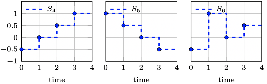
Figure 4: Discrete-time signals in Example 6.

TABLE I: Traditional and weighted AGM robustness for different values of $\gamma$ in $\varpi(t)=\gamma^{(t-1)}$ for $\varphi={\mathbf{F}}^{\varpi}_{[0,3]}(S\geq 0)$

Signal	$\rho$	$\eta$	$\eta^{w},\gamma=0.9$	$\eta^{w},\gamma=0.5$	$\eta^{w},\gamma=0.1$
$S_{4}$	1	0.375	0.330	0.133	0.005
$S_{5}$	1	0.375	0.420	0.666	0.945
$S_{6}$	1	0.375	0.367	0.300	0.090

Example 7

Consider Example 1 with trajectories $c_{1}$ and $c_{2}$. Assuming $\varpi=\mathbf{1}$, from (11) we have $\eta^{w}(\varphi_{2},c_{1})=\eta^{w}(\varphi_{3},c_{2})=-\frac{2}{8}$. Similarly, for the overall specification $\varphi$, we have $\eta^{w}(\varphi,c_{1})=\sum_{i=1}^{3}{\bar{p}_{i}{[\eta^{w}(\varphi_{i},c_{1})]_{-}}}={\bar{p}_{2}\;\eta^{w}(\varphi_{2},c_{1})}$ and $\eta^{w}(\varphi,c_{2})=\bar{p}_{3}\;\eta^{w}(\varphi_{3},c_{2})$. If $p_{2}=p_{3}$, satisfaction of both $\varphi_{1}$ and $\varphi_{2}$ will have the same importance. Thus, $c_{1}$ and $c_{2}$ have the same robustness. Assume avoiding Blocked is more important than staying in the lane. By choosing $p_{2}>p_{3}$, we can emphasize the importance of $\varphi_{2}$. As a result, $\bar{p}_{2}>\bar{p}_{3}$ and $\eta^{w}(\varphi,c_{1})<\eta^{w}(\varphi,c_{2})<0$. Since the satisfaction of all the sub-formulae is not feasible, $c_{2}$ is the minimally violating trajectory (compared to $c_{1}$).

V Synthesis Using Weighted Robustness

The soundness property of the weighted robustness $r^{w}$ allows us to reformulate the synthesis problem (6) as:

$$\small\begin{array}[]{c}\mathbf{u}^{*}={\mathop{\mathrm{argmax}}}_{u(t)\in\mathcal{U}}\;r^{w}(\varphi,\mathbf{q}(q_{0},\mathbf{u}))-\lambda\;J(u(t),q(t))\\ \text{s.t.}\;\;\;\;\text{dynamics}\;\;\eqref{eq:dynamics}\;\;\text{are satisfied},\\ {}r^{w}(\varphi,\mathbf{q}(q_{0},\mathbf{u}))>\epsilon,\end{array}\vspace{-2pt}$$ (12)

where $\epsilon\geq 0$ is the lower bound of the satisfaction margin (soundness threshold) as captured by the weighted generalization of the recursive STL robustness [9]. Since the weighted robustness of wSTL is defined as a generalization of an unweighted recursive STL robustness, previous robustness optimization frameworks can be adapted to solve (12).

We consider a discrete-time system with a finite time $T$ and assume the control policy to be synthesized is a discrete ordered sequence $\mathbf{u}=\small{u(0)u(1)\cdots u(T-1)}$. We use a gradient-based optimization to solve (12). Note that the weights do not increase the computation time compared to the unweighted robustness optimization. $r^{w}$ is iteratively maximized by updating the input variable $u(t)$ at each time $t$ proportional to the gradient of $r^{w}$ such that $\small{u(t)^{l+1}\leftarrow u(t)^{l}+\alpha^{l}\;\nabla r^{w}}$, where $l$ is optimization iteration, $\alpha^{l}$ is step size and $\nabla r^{w}=\frac{\partial r^{w}(\varphi,\mathbf{q}(q_{0},\mathbf{u}))}{\partial u(t)}$ [23]. Therefore, depending on the aggregation functions in $r^{w}$, the weights $p$ and $\varpi$ associated with $\varphi$ affect the gradient and optimization. A similar synthesis framework can be applied to continuous-time systems with a Zeroth-Order Hold (ZOH) input [17].

VI Case Study

Consider a discrete-time nonlinear dynamical system as:

$$\begin{array}[]{l}x(t+1)=x(t)+\cos\theta(t)v(t),\\ y(t+1)=y(t)+\sin\theta(t)v(t),\\ \theta(t+1)=\theta(t)+v(t)w(t),\end{array}\vspace{-3pt}$$ (13)

and a task “Eventually visit A or B within $[1,10]$ and eventually visit C within $[11,20]$ and Always avoid Unsafe and Always stay inside Boundary” given by wSTL formula:

$$\begin{array}[]{l}\varphi=(\mathbf{F}_{[1,10]}\;(\textit{A}\vee^{p}\textit{B}))\;\wedge(\mathbf{F}_{[11,20]}\textit{ C})\\ \;\;\;\;\;\;\;\;\;\;\;\wedge\;(\mathbf{G}_{[1,20]}\;\neg\textit{Unsafe})\;\wedge(\mathbf{G}_{[1,20]}\;\textit{Boundary}),\end{array}\vspace{-3pt}$$ (14)

where $\textit{A}=[7,9]\times[1,3]$ or $\textit{B}=[1,3]\times[7,9]$ and $\textit{C}=[7,9]^{2}$ are regions to be sequentially visited within the associated deadlines, $\textit{Unsafe}=[3,6]^{2}$ and $\textit{Boundary}=[0,10]^{2}$. $q=[x,y,\theta]$ is state vector with initial state $q_{0}=[1,1,\pi/4]$, $u=[v,w]$ is the input vector with $\mathcal{U}=[-2,2]^{2}$, and cost function is $J=\frac{1}{2}\sum_{t=0}^{T-1}{\|u(t)\|^{2}}$ with $T=20$, $\lambda=0.05$ in (12).

&

Figure 5: Trajectories from the synthesized control $\mathbf{u}^{*}$ satisfy $\varphi$ and minimize the cost. $p_{\textit{A}}>p_{\textit{B}}$ (left), $p_{\textit{A}}<p_{\textit{B}}$ (right).

By defining $\otimes^{\land}(p,x)=\widetilde{\min}_{i=1:N}\{\big{(}(\frac{1}{2}-\bar{p_{i}})\mathop{\mathrm{sign}}(x_{i})+\frac{1}{2}\big{)}\cdot x_{i}\}$, $\oplus^{\lor}(p,x)=\widetilde{\max}_{i=1:N}\{\big{(}-(\frac{1}{2}-\bar{p_{i}})\mathop{\mathrm{sign}}(x_{i})+\frac{1}{2}\big{)}\cdot x_{i}\}$ from (3) (similarly for $\oplus^{\mathbf{G}}$ and $\oplus^{\mathbf{F}}$), and approximating $\mathop{\mathrm{sign}}$ by $\mathop{\mathrm{sign}}(x)\simeq\tanh({\beta x})$, we obtain the weighted sound smooth robustness of [15], which is adjustable to a desired locality and masking level. Fig. VI shows trajectories obtained from optimizing (12) considering the weighted robustness of [15] with $\beta=10$, achieved up to the same termination criteria with different priorities for visiting A or B as $p_{\textit{A}}=2$, $p_{\textit{B}}=1$ (left), and $p_{\textit{A}}=1$, $p_{\textit{B}}=2$ (right). The optimization is implemented in Matlab using the SQP optimizer and takes about $1.2$ seconds on a Mac with 2.5 GHz Core i7 CPU 16GB RAM. For the given symmetrical configuration and initial state, optimizing the weighted robustness ensures that the optimal trajectory visits the higher priority region A or B as chosen by the disjunction aggregator priorities $p$.

VII Conclusion And Future Work

We presented an extension of STL to improve its expressivity by encoding the importance or priorities of sub-formulae and time in a formula. The new formalism, called wSTL, is advantageous especially in the problems where satisfaction of a formula is not feasible, and as a result, the less important sub-formulae or time are preferred to be violated to guarantee that more important ones are satisfied. The weighted robustness associated with wSTL also improved the optimal behavior in a control synthesis framework solved using gradient techniques where prioritized tasks were critical. Future work will investigate computationally efficient implementations of the wSTL robustness optimization, and learning frameworks for systematic design of weights to capture hierarchies of wSTL formulae consistently.

References

- [1] C. Baier and J. Katoen, Principles of model checking. The MIT Press, 2008.
- [2] C. Belta, B. Yordanov, and E. A. Gol, Formal methods for discrete-time dynamical systems. Springer, 2017, vol. 89.
- [3] P. Tabuada, Verification and control of hybrid systems: a symbolic approach. Springer Science & Business Media, 2009.
- [4] R. Alur, T. A. Henzinger, and E. D. Sontag, Hybrid systems III: verification and control. Springer, 1996, vol. 3.
- [5] O. Maler and D. Nickovic, “Monitoring temporal properties of continuous signals,” in Formal Techniques, Modelling and Analysis of Timed and Fault-Tolerant Systems. Springer, 2004, pp. 152–166.
- [6] N. Mehdipour, D. Briers, I. Haghighi, C. M. Glen, M. L. Kemp, and C. Belta, “Spatial-temporal pattern synthesis in a network of locally interacting cells,” in IEEE Conference on Decision and Control (CDC). IEEE, 2018, pp. 3516–3521.
- [7] S. Saha and A. A. Julius, “An MILP approach for real-time optimal controller synthesis with metric temporal logic specifications,” in American Control Conference (ACC). IEEE, 2016, pp. 1105–1110.
- [8] V. Raman, A. Donzé, M. Maasoumy, R. M. Murray, A. Sangiovanni-Vincentelli, and S. A. Seshia, “Model predictive control with signal temporal logic specifications,” in 53rd IEEE Conference on Decision and Control. IEEE, 2014, pp. 81–87.
- [9] Y. V. Pant, H. Abbas, and R. Mangharam, “Smooth operator: Control using the smooth robustness of temporal logic,” in Conference on Control Technology and Applications. IEEE, 2017, pp. 1235–1240.
- [10] C. Belta and S. Sadraddini, “Formal methods for control synthesis: An optimization perspective,” Annual Review of Control, Robotics, and Autonomous Systems, vol. 2, pp. 115–140, 2019.
- [11] A. Donzé and O. Maler, “Robust satisfaction of temporal logic over real-valued signals,” in International Conference on Formal Modeling and Analysis of Timed Systems. Springer, 2010, pp. 92–106.
- [12] L. Lindemann and D. V. Dimarogonas, “Robust control for signal temporal logic specifications using discrete average space robustness,” Automatica, vol. 101, pp. 377–387, 2019.
- [13] I. Haghighi, N. Mehdipour, E. Bartocci, and C. Belta, “Control from signal temporal logic specifications with smooth cumulative quantitative semantics,” in IEEE 58th Conference on Decision and Control (CDC). IEEE, 2019, pp. 4361–4366.
- [14] P. Varnai and D. V. Dimarogonas, “On Robustness Metrics for Learning STL Tasks,” in American Control Conference (ACC), 2020, pp. 5394–5399.
- [15] Y. Gilpin, V. Kurtz, and H. Lin, “A Smooth Robustness Measure of Signal Temporal Logic for Symbolic Control,” IEEE Control Systems Letters, vol. 5, no. 1, pp. 241–246, 2021.
- [16] N. Mehdipour, C.-I. Vasile, and C. Belta, “Arithmetic-geometric mean robustness for control from signal temporal logic specifications,” in American Control Conference (ACC). IEEE, 2019, pp. 1690–1695.
- [17] N. Mehdipour, C. Vasile, and C. Belta, “Average-based robustness for continuous-time signal temporal logic,” in 58th Conference on Decision and Control (CDC). IEEE, 2019, pp. 5312–5317.
- [18] P. Tabuada and D. Neider, “Robust Linear Temporal Logic,” in 25th EACSL Annual Conference on Computer Science Logic (CSL 2016), vol. 62, 2016, pp. 10:1–10:21.
- [19] C.-I. Vasile, J. Tumova, S. Karaman, C. Belta, and D. Rus, “Minimum-violation scltl motion planning for mobility-on-demand,” in International Conference on Robotics and Automation (ICRA). IEEE, 2017, pp. 1481–1488.
- [20] R. Dimitrova, M. Ghasemi, and U. Topcu, “Maximum realizability for linear temporal logic specifications,” in International Symposium on Automated Technology for Verification and Analysis. Springer, 2018, pp. 458–475.
- [21] B. Hoxha, A. Dokhanchi, and G. Fainekos, “Mining parametric temporal logic properties in model-based design for cyber-physical systems,” International Journal on Software Tools for Technology Transfer, vol. 20, no. 1, pp. 79–93, 2018.
- [22] C.-I. Vasile, D. Aksaray, and C. Belta, “Time window temporal logic,” Theoretical Computer Science, vol. 691, pp. 27–54, 2017.
- [23] D. P. Bertsekas, Nonlinear programming. Athena scientific Belmont, 1999.