Discontinuous Constituent Parsing as Sequence Labeling
Abstract
This paper reduces discontinuous parsing to sequence labeling. It first shows that existing reductions for constituent parsing as labeling do not support discontinuities. Second, it fills this gap and proposes to encode tree discontinuities as nearly ordered permutations of the input sequence. Third, it studies whether such discontinuous representations are learnable. The experiments show that despite the architectural simplicity, under the right representation, the models are fast and accurate.111https://github.com/aghie/disco2labels
1 Introduction
Discontinuous constituent parsing studies how to generate phrase-structure trees of sentences coming from non-configurational languages Johnson (1985), where non-consecutive tokens can be part of the same grammatical function (e.g. non-consecutive terms belonging to the same verb phrase). Figure 1 shows a German sentence exhibiting this phenomenon. Discontinuities happen in languages that exhibit free word order such as German or Guugu Yimidhirr Haviland (1979); Johnson (1985), but also in those with high rigidity, e.g. English, whose grammar allows certain discontinuous expressions, such as wh-movement or extraposition Evang and Kallmeyer (2011). This makes discontinuous parsing a core computational linguistics problem that affects a wide spectrum of languages.
There are different paradigms for discontinuous phrase-structure parsing, such as chart-based parsers Maier (2010); Corro (2020), transition-based algorithms Coavoux and Crabbé (2017); Coavoux and Cohen (2019) or reductions to a problem of a different nature, such as dependency parsing Hall and Nivre (2008); Fernández-González and Martins (2015). However, many of these approaches come either at a high complexity or low speed, while others give up significant performance to achieve an acceptable latency Maier (2015).
Related to these research aspects, this work explores the feasibility of discontinuous parsing under the sequence labeling paradigm, inspired by Gómez-Rodríguez and Vilares (2018)’s work on fast and simple continuous constituent parsing. We will focus on tackling the limitations of their encoding functions when it comes to analyzing discontinuous structures, and include an empirical comparison against existing parsers.

Contribution
(i) The first contribution is theoretical: to reduce constituent parsing of free word order languages to a sequence labeling problem. This is done by encoding the order of the sentence as (nearly ordered) permutations. We present various ways of doing so, which can be naturally combined with the labels produced by existing reductions for continuous constituent parsing. (ii) The second contribution is a practical one: to show how these representations can be learned by neural transducers. We also shed light on whether general-purpose architectures for NLP tasks Devlin et al. (2019); Sanh et al. (2019) can effectively parse free word order languages, and be used as an alternative to ad-hoc algorithms and architectures for discontinuous constituent parsing.
2 Related work
Discontinuous phrase-structure trees can be derived by expressive formalisms such as Multiple Context Free Grammmars Seki et al. (1991) (MCFGs) or Linear Context-Free Rewriting Systems (LCFRS) Vijay-Shanker et al. (1987). MCFGs and LCFRS are essentially an extension of Context-Free Grammars (CFGs) such that non-terminals can link to non-consecutive spans. Traditionally, chart-based parsers relying on this paradigm commonly suffer from high complexity Evang and Kallmeyer (2011); Maier and Kallmeyer (2010); Maier (2010). Let be the block degree, i.e. the number of non-consecutive spans than can be attached to a single non-terminal; the complexity of applying CYK (after binarizing the grammar) would be (Seki et al., 1991), which can be improved to if the parser is restricted to well-nested LCFRS (Gómez-Rodríguez et al., 2010), and Maier (2015) discusses how for a standard discontinuous treebank, (in contrast to in CFGs). Recently, Corro (2020) presents a chart-based parser for that can run in , which is equivalent to the running time of a continuous chart parser, while covering 98% of the discontinuities. Also recently, Stanojević and Steedman (2020) present an LCFRS parser with that runs in worst-case time, where is the number of unique non-terminal symbols, but in practice they show that the empirical running time is among the best chart-based parsers.
Differently, it is possible to rely on the idea that discontinuities are inherently related to the location of the token in the sentence. In this sense, it is possible to reorder the tokens while still obtaining a grammatical sentence that could be parsed by a continuous algorithm. This is usually achieved with transition-based parsing algorithms and the swap transition Nivre (2009) which switches the topmost elements in the stack. For instance, Versley (2014) uses this transition to adapt an easy-first strategy Goldberg and Elhadad (2010) for dependency parsing to discontinuous constituent parsing. In a similar vein, Maier (2015) builds on top of a fast continuous shift-reduce constituent parser Zhu et al. (2013), and incorporates both standard and bundled swap transitions in order to analyze discontinuous constituents. Maier’s system produces derivations of up to a length of given a sentence of length . More efficiently, Coavoux and Crabbé (2017) present a transition system which replaces swap with a gap transition. The intuition is that a reduction does not need to be always applied locally to the two topmost elements in the stack, and that those two items can be connected, despite the existence of a gap between them, using non-local reductions. Their algorithm ensures an upper-bound of transitions.222Or alternatively , if we apply additional constraints to the gap transition and transitions following a shift action. However this comes at a cost of not being able to map more than gaps within the same discontinuous constituent. With a different optimization goal, Stanojević and Alhama (2017) removed the traditional reliance of discontinuous parsers on averaged perceptrons and hand-crafted features for a recursive neural network approach that guides a swap-based system, with the capacity to generate contextualized representations. Coavoux and Cohen (2019) replace the stack used in transition-based systems with a memory set containing the created constituents. This model allows interactions between elements that are not adjacent, without the swap transition, to create a new (discontinuous) constituent. Trained on a 2 stacked BiLSTM transducer, the model is guaranteed to build a tree with in 4-2 transitions, given a sentence of length .
A middle ground between explicit constituent parsing algorithms and this paper is the work based on transformations. For instance, Hall and Nivre (2008) convert constituent trees into a non-linguistic dependency representation that is learned by a transition-based dependency parser, to then map its output back to a constituent tree. A similar approach is taken by Fernández-González and Martins (2015), but they proposed a more compact representation that leads to a much reduced set of output labels. Other authors such as Versley (2016) propose a two-step approach that approximates discontinuous structure trees by parsing context-free grammars with generative probabilistic models and transforming them to discontinuous ones. Corro et al. (2017) cast discontinuous phrase-structure parsing into a framework that jointly performs supertagging and non-projective dependency parsing by a reduction to the Generalized Maximum Spanning Arborescence problem Myung et al. (1995). The recent work by Fernández-González and Gómez-Rodríguez (2020a) can be also framed within this paradigm. They essentially adapt the work by Fernández-González and Martins (2015) and replace the averaged perceptron classifier with pointer networks Vinyals et al. (2015), adressing the problem as a sequence-to-sequence task (for dependency parsing) whose output is then mapped back to the constituent tree. And next, Fernández-González and Gómez-Rodríguez (2020b) extended pointer networks with multitask learning to jointly predict constituent and dependency outputs.
In this context, the closest work to ours is the reduction proposed by Gómez-Rodríguez and Vilares (2018), who cast continuous constituent parsing as sequence labeling.333Related to constituent parsing and sequence labeling, there are two related papers that made early efforts (although not a full reduction of the former to the latter) and need to be credited too. Ratnaparkhi (1999) popularized maximum entropy models for parsing and combined a sequence labeling process that performs PoS-tagging and chunking with a set of shift-reduce-like operations to complete the constituent tree. In a related line, Collobert (2011) proposed a multi-step approach consisting of passes over the input sentence, where each of them tags every word as being part of a constituent or not at one of the levels of the tree, using a IOBES scheme. In the next sections we build on top of their work and: (i) analyze why their approach cannot handle discontinuous phrases, (ii) extend it to handle such phenomena, and (iii) train functional sequence labeling discontinuous parsers.
3 Preliminaries
Let be an input sequence of tokens, and the set of (continuous) constituent trees for sequences of length ; Gómez-Rodríguez and Vilares (2018) define an encoding function to map continuous constituent trees into a sequence of labels of the same length as the input. Each label, , is composed of three components :
-
•
encodes the number of levels in the tree in common between a word and . To obtain a manageable output vocabulary space, is actually encoded as the difference , with . We denote by the absolute number of levels represented by . i.e. the total levels in common shared between a word and its next one.
-
•
represents the lowest non-terminal symbol shared between and at level .
-
•
encodes a leaf unary chain, i.e. non-terminals that belong only to the path from the terminal to the root.444Intermediate unary chains are compressed into a single non-terminal and treated as a regular branches. Note that cannot encode this information in (), as these components always represent common information between and .
Figure 2 illustrates the encoding on a continuous example.
Incompleteness for discontinuous phrase structures
Gómez-Rodríguez and Vilares proved that is complete and injective for continuous trees. However, it is easy to prove that its validity does not extend to discontinuous trees, by using a counterexample. Figure 3 shows a minimal discontinuous tree that cannot be correctly decoded.
The inability to encode discontinuities lies on the assumption that will always be attached to a node belonging to the path from the root to ( is then used to specify the location of that node in the path). This is always true in continuous trees, but not in discontinuous trees, as can be seen in Figure 3 where is the child of a constituent that does not lie in the path from to .
4 Encoding nearly ordered permutations
Next, we fill this gap to address discontinuous parsing as sequence labeling. We will extend the encoding to the set of discontinuous constituent trees, which we will call . The key to do this relies on a well-known property: a discontinuous tree can be represented as a continuous one using an in-order traversal that keeps track of the original indexes (e.g. the trees at the left and the right in Figure 4).555This is the discbracket format. See: https://discodop.readthedocs.io/en/latest/fileformats.html We will call this tree the (canonical) continuous arrangement of , .
Thus, if given an input sentence we can generate the position of every word as a terminal in , the existing encodings to predict continuous trees as sequence labeling could be applied on . In essence, this is learning to predict a permutation of . As introduced in §2, the concept of location of a token is not a stranger in transition-based discontinuous parsing, where actions such as swap switch the position of two elements in order to create a discontinuous phrase. We instead propose to explore how to handle this problem in end-to-end sequence labeling fashion, without relying on any parsing structure nor a set of transitions.
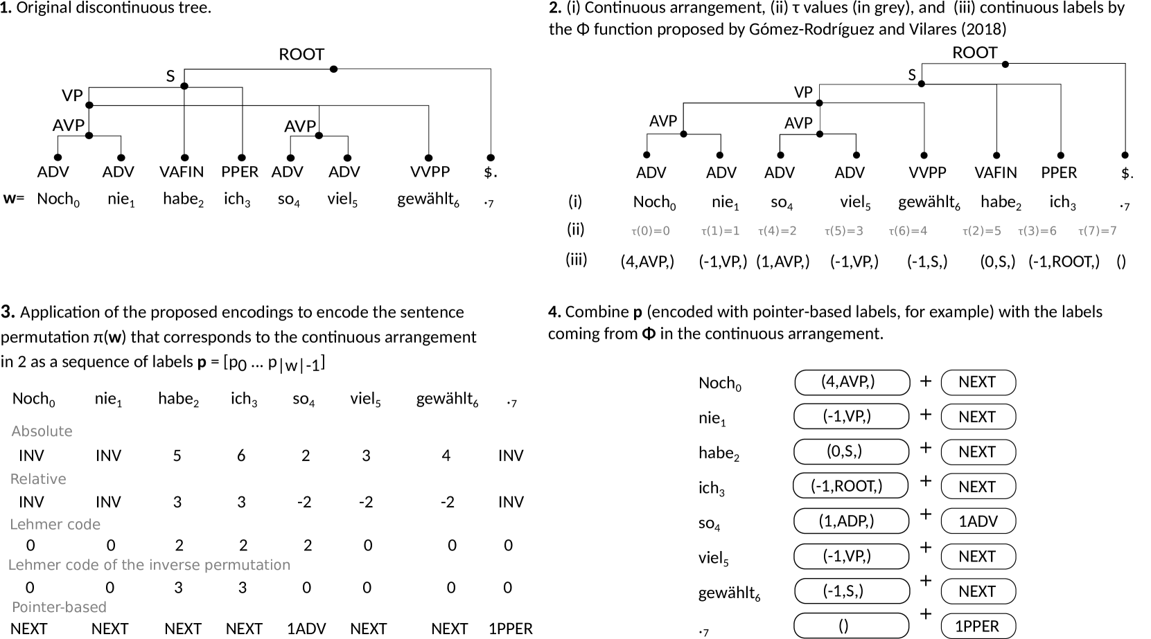
To do so, first we denote by the permutation that maps the position of a given in into its position as a terminal node in .666Permutations are often defined as mappings from the element at a given position to the element that replaces it, but for our purpose, we believe that the definition as a function from original positions to rearranged positions (following, e.g., (O’Donnell et al., 2007)) is more straightforward. From this, one can derive , a function that encodes a permutation of in such way that its phrase structure does not have crossing branches. For continuous trees, and are identity permutations. Then, we extend the tree encoding function to where is enriched with a fourth component such that , where is a discrete symbol such that the sequence of ’s encodes the permutation (typically each will be an encoding of , i.e. the position of in the continuous arrangement, although this need not be true in all encodings, as will be seen below).
The crux of defining a viable encoding for discontinuous parsing is then in how we encode as a sequence of values , for . While the naive approach would be the identity encoding (), we ideally want an encoding that balances minimizing sparsity (by minimizing infrequently-used values) and maximizing learnability (by being predictable). To do so, we will look for encodings that take advantage of the fact that discontinuities in attested syntactic structures are mild (Maier and Lichte, 2011), i.e., in most cases, . In other words, permutations corresponding to real syntactic trees tend to be nearly ordered permutations. Based on these principles, we propose below a set of concrete encodings, which are also depicted on an example in Figure 4. All of them handle multiple gaps (a discontinuity inside a discontinuity) and cover 100% of the discontinuities. Even if this has little effect in practice, it is an interesting property compared to algorithms that limit the number of gaps they can address Coavoux and Cohen (2019); Corro (2020).
Absolute-position
For every token , only if . Otherwise, we use a special label INV, which represents that the word is a fixed point in the permutation, i.e., it occupies the same place in the sentence and in the continuous arrangement.
Relative-position
If , then ; otherwise, we again use the INV label.
Lehmer code
Laisant (1888); Lehmer (1960) In combinatorics, let be a sorted sequence of objects, a Lehmer code is a sequence that encodes one of the permutations of , namely . The idea is intuitive: let be the subsequence of objects from that remain available after we have permuted the first objects to achieve the permutation , then equals the (zero-based) position in of the next object to be selected. For instance, given = and a valid permutation = , then = . Note that the identity permutation would be encoded as a sequence of zeros.
In the context of discontinuous parsing and encoding , can be seen as the input sentence where is encoded by . The Lehmer code is particularly suitable for this task in terms of compression, as in most of the cases we expect (nearly) ordered permutations, which translates into the majority of elements of being zero.777For a continuous tree, . However, this encoding poses some potential learnability problems. The root of the problem is that does not necessarily encode , but where is the index of the word that occupies the th position in the continuous arrangement (i.e., ). In other words, this encoding is expressed following the order of words in the continuous arrangement rather than the input order, causing a non-straightforward mapping between input words and labels. For instance, in the previous example, does not encode the location of the object =2 but that of =3.
Lehmer code of the inverse permutation
To ensure that each encodes , we instead interpret as meaning that should fill the th currently remaining blank in a sequence that is initialized as a sequence of blanks, i.e. . For instance, let be the original input and its desired continuous arrangement. At the first and second steps, and occupy the first available blanks (so ), generating partial arrangements of the form and . Then, would need to fill the third empty blank (so ), and we obtain . After that, and occupy the first available blank (so ). Thus, we obtain the desired arrangement , and the encoding is . It is easy to check that this produces the Lehmer code for the inverse permutation to . Hence, it shares the property that the identity permutation is encoded by a sequence of zeros, but it is more straightforward for our purposes as each encodes information about , the target position of in the continuous arrangement. Note that this and the Lehmer code coincide iff is a self-conjugate permutation (i.e., a conjugate that is its own inverse, see (Muir, 1891)), of which the identity is a particular case.
Pointer-based encoding
When encoding , the previous encodings generate the position for the target word, but they do not really take into account the left-to-right order in which sentences are naturally read,888We use left-to-right in an informal sense to mean that sentences are processed in linear temporal order. Of course, not all languages follow a left-to-right script. nor they are linguistically inspired.
In particular, informally speaking, in human linguistic processing (i.e. when a sentence is read from left to right) we could say that a discontinuity is processed when we read a word that continues a phrase other than that of the previously read word. For example, for the running example sentence (Figure 4), from an abstract standpoint we know that there is a discontinuity because , i.e., “nie” and “habe” are not contiguous in the continuous arrangement of the tree. However, in a left-to-right processing of the sentence, there is no way to know the final desired position of “habe” () until we read the words “so viel gewählt”, which go before it in the continuous arrangement. Thus, the requirement of the previous four encodings to assign a concrete non-default value to the s associated with “habe” and “ich” is not too natural from an incremental reading standpoint, as learning requires information that can only be obtained by looking to the right of . This can be avoided by using a model that just processes “Noch nie habe ich” as if it were a continuous subtree (in fact, if we removed “so viel gewählt” from the sentence, the tree would be continuous). Then, upon reading “so”, the model notices that it continues the phrase associated with “nie” and not with “ich”, and hence inserts it after “nie” in the continuous arrangement.
This idea of incremental left-to-right processing of discontinuities is abstracted in the form of a pointer that signals the last terminal in the current continuous arrangement of the constituent that we are currently filling. That said, to generate the labels this approach needs to consider two situations:
-
•
If is to be inserted right after (this situation is characterized by ). This case is abstracted by a single label, =NEXT, that means to insert at the position currently pointed by , and then update , where the function is defined as . can informally be described as a tentative value of , corresponding to the position of in the part of the continuous arrangement that involves the substring .
-
•
Otherwise, should be inserted after some with , which means there is a discontinuity and that the current pointer is no longer valid and needs to be first updated to point to . To generate the label we use a tuple that indicates that the predecessor of in is the th preceding word in with the PoS tag . After that, we update the pointer to . While this encoding could work with PoS-tag-independent relative offsets, or any word property, the PoS-tag-based indexing provides linguistic grounding and is consistent with sequence labeling encodings that have obtained good results in dependency parsing Strzyz et al. (2019).
Pointer-based encoding (with simplified PoS tags)
A pointer-based variant where the PoS tags in are simplified (e.g. NNS NN). The mapping is described in Appendix A.1. Apart from reducing sparsity, the idea is that a discontinuity is not so much influenced by specific information but by the coarse morphological category.
Ill-formed permutations are corrected with post-processing, following Appendix A.2, to ensure that the derived permutations contain all word indexes.
4.1 Limitations
The encodings are complete under the assumption of an infinite label vocabulary. In practice, training sets are finite and this could cause the presence of unseen labels in the test set, especially for the integer-based label components:999This is a general limitation also present in previous parsing as sequence labeling approaches (e.g. Gómez-Rodríguez and Vilares (2018)), and could potentially happen with any label component, e.g. predicting the non-terminal symbol. However, it is very unlikely that a non-terminal symbol has not been observed in the training set. Also, chart- and transition-based parsers would suffer from this same limitation. the levels in common () and the label component that encodes . However, as illustrated in Appendix A.3, an analysis on the corpora used in this work shows that the presence of unseen labels in the test set is virtually zero.
5 Sequence labeling frameworks
To test whether these encoding functions are learnable by parametrizable functions, we consider different sequence labeling architectures. We will be denoting by encoder a generic, contextualized encoder that for every word generates a hidden vector conditioned on the sentence, i.e. encoder()=. We use a hard-sharing multi-task learning architecture Caruana (1997); Vilares et al. (2019) to map every to four 1-layered feed-forward networks, followed by softmaxes, that predict each of the components of . Each task’s loss is optimized using categorical cross-entropy and the final loss computed as . We test four encoders, which we briefly review but treat as black boxes. Their number of parameters and the training hyper-parameters are listed in Appendix A.4.
Transducers without pretraining
We try (i) a 2-stacked BiLSTM Hochreiter and Schmidhuber (1997); Yang and Zhang (2018) where the generation of is conditioned on the left and right context. (ii) We also explore a Transformer encoder Vaswani et al. (2017) with 6 layers and 8 heads. The motivation is that we believe that the multi-head attention mechanism, in which a word attends to every other word in the sentence, together with positional embeddings, could be beneficial to detect discontinuities. In practice, we found training these transformer encoders harder than training BiLSTMs, and that obtaining a competitive performance required larger models, smaller learning rates, and more epochs (see also Appendix A.4).
The input to these two transducers is a sequence of vectors composed of: a pre-trained word embedding Ling et al. (2015) further fine-tuned during training, a PoStag embedding, and a second word embedding trained with a character LSTM. Additionally, the Transformer uses positional embeddings to be aware of the order of the sentence.
Transducers with pretraining
Previous work on sequence labeling parsing Gómez-Rodríguez and Vilares (2018); Strzyz et al. (2019) has shown that although effective, the models lag a bit behind state-of-the-art accuracy. This setup, inspired in Vilares et al. (2020), aims to evaluate whether general purpose NLP architectures can achieve strong results when parsing free word order languages. In particular, we fine-tune (iii) pre-trained BERT Devlin et al. (2019), and (iv) pre-trained DistilBERT Sanh et al. (2019). BERT and DistilBERT map input words to sub-word pieces Wu et al. (2016). We align each word with its first sub-word, and use their embedding as the only input for these models.
6 Experiments
Setup
For English, we use the discontinuous Penn Treebank (DPTB) by Evang and Kallmeyer (2011). For German, we use TIGER and NEGRA Brants et al. (2002); Skut et al. (1997). We use the splits by Coavoux and Cohen (2019) which in turn follow the Dubey and Keller (2003) splits for the NEGRA treebank, the Seddah et al. (2013) splits for TIGER, and the standard splits for (D)PTB (Sections 2 to 21 for training, 22 for development and 23 for testing). See also Appendix A.5 for more detailed statistics. We consider gold and predicted PoS tags. For the latter, the parsers are trained on predicted PoS tags, which are generated by a 2-stacked BiLSTM, with the hyper-parameters used to train the parsers. The PoS tagging accuracy (%) on the dev/test is: DPTB 97.5/97.7, TIGER 98.7/97.8 and NEGRA 98.6/98.1. BERT and DistilBERT do not use PoS tags as input, but when used to predict the pointer-based encodings, they are required to decode the labels into a parenthesized tree, causing variations in the performance.101010The rest of BERT models do not require PoS tags at all. Table 1 shows the number of labels per treebank.
| Label Component | #Labels | ||
|---|---|---|---|
| TIGER | NEGRA | DPTB | |
| 22 | 19 | 34 | |
| 93 | 56 | 137 | |
| 15 | 4 | 56 | |
| as absolute-position | 129 | 110 | 98 |
| as relative-position | 105 | 90 | 87 |
| as Lehmer | 39 | 34 | 27 |
| as inverse Lehmer | 68 | 57 | 61 |
| as pointer-based | 122 | 99⋆ | 110⋆ |
| as pointer-based simplified | 81 | 65 | 83⋆ |
| Encoding | Transducer | TIGER | NEGRA | DPTB | |||
|---|---|---|---|---|---|---|---|
| F1 | Disco F-1 | F1 | Disco F-1 | F1 | Disco F-1 | ||
| Absolute-position | BiLSTM | 75.2 | 12.4 | 72.8 | 12.8 | 86.0 | 10.7 |
| Relative-position | BiLSTM | 77.7 | 20.4 | 73.4 | 14.9 | 86.6 | 15.2 |
| Lehmer | BiLSTM | 81.6 | 33.4 | 76.8 | 26.2 | 88.4 | 30.7 |
| Inverse Lehmer | BiLSTM | 83.2 | 41.6 | 77.3 | 27.0 | 88.9 | 36.0 |
| Pointer-based | BiLSTM | 84.4 | 49.0 | 79.8 | 36.7 | 89.9 | 47.9 |
| Pointer-based simplified | BiLSTM | 84.6 | 48.7 | 79.8 | 38.1 | 90.0 | 46.3 |
| Absolute-position | Transformer | 81.9 | 38.3 | 75.3 | 25.4 | 87.5 | 25.8 |
| Relative-position | Transformer | 77.0 | 20.2 | 71.4 | 13.5 | 86.8 | 16.4 |
| Lehmer | Transformer | 82.6 | 38.5 | 75.4 | 21.4 | 88.1 | 24.8 |
| Inverse Lehmer | Transformer | 85.3 | 47.9 | 77.7 | 30.8 | 88.7 | 35.7 |
| Pointer-based | Transformer | 86.0 | 51.2 | 79.8 | 38.8 | 90.2 | 46.7 |
| Pointer-based simplified | Transformer | 86.0 | 50.4 | 80.6 | 42.5 | 90.2 | 46.2 |
| Absolute-position | BERT | 86.4 | 47.4 | 80.7 | 25.3 | 89.4 | 20.7 |
| Relative-position | BERT | 83.8 | 29.5 | 78.7 | 18.0 | 89.8 | 22.5 |
| Lehmer | BERT | 86.9 | 43.6 | 82.6 | 30.4 | 91.0 | 36.3 |
| Inverse Lehmer | BERT | 86.9 | 50.3 | 83.3 | 34.6 | 90.9 | 38.1 |
| Pointer-based | BERT | 89.2 | 57.8 | 86.4 | 52.0 | 92.2 | 53.8 |
| Pointer-based simplified | BERT | 89.2 | 59.7 | 86.4 | 49.3 | 92.0 | 50.9 |
| Absolute-position | DistilBERT | 82.0 | 30.6 | 75.6 | 19.0 | 88.2 | 17.7 |
| Relative-position | DistilBERT | 80.3 | 21.8 | 74.3 | 12.3 | 88.1 | 18.4 |
| Lehmer | DistilBERT | 83.3 | 32.8 | 77.6 | 21.6 | 89.5 | 33.0 |
| Inverse Lehmer | DistilBERT | 84.2 | 39.7 | 78.5 | 25.3 | 89.7 | 34.2 |
| Pointer-based | DistilBERT | 86.8 | 51.6 | 82.8 | 42.7 | 90.7 | 46.3 |
| Pointer-based simplified | DistilBERT | 87.0 | 54.7 | 82.7 | 40.5 | 90.7 | 43.1 |
Metrics
We report the F-1 labeled bracketing score for all and discontinuous constituents, using discodop van Cranenburgh et al. (2016)111111http://github.com/andreasvc/disco-dop and the proper.prm parameter file. Model selection is based on overall bracketing F1- score.
6.1 Results
Table 2 shows the results on the dev sets for all encodings and transducers. The tendency is clear showing that the pointer-based encodings obtain the best results. The pointer-based encoding with simplified PoS tags does not lead however to clear improvements, suggesting that the models can learn the sparser original PoS tags set. For the rest of encodings we also observe interesting tendencies. For instance, when running experiments using stacked BiLSTMs, the relative encoding performs better than the absolute one, which was somehow expected as the encoding is less sparse. However, the tendency is the opposite for the Transformer encoders (including BERT and DistilBERT), especially for the case of discontinuous constituents. We hypothesize this is due to the capacity of Transformers to attend to every other word through multi-head attention, which might give an advantage to encode absolute positions over BiLSTMs, where the whole left and right context is represented by a single vector. With respect to the Lehmer and Lehmer of the inverse permutation encodings, the latter performs better overall, confirming the bigger difficulties for the tested sequence labelers to learn Lehmer, which in some cases has a performance even close to the naive absolute-positional encoding (e.g. for TIGER using the vanilla Transformer encoder and BERT). As introduced in §4, we hypothesize this is caused by the non-straightforward mapping between words and labels (in the Lehmer code the label generated for a word does not necessarily contain information about the position of such word in the continuous arrangement).
In Table 3 we compare a selection of our models against previous work using both gold and predicted PoS tags. In particular, we include: (i) models using the pointer-based encoding, since they obtained the overall best performance on the dev sets, and (ii) a representative subset of encodings (the absolute positional one and the Lehmer code of the inverse permutation) trained with the best performing transducer. Additionally, for the case of the (English) DPTB, we also include experiments using a bert-large model, to shed more light on whether the size of the networks is playing a role when it comes to detect discontinuities. Additionally, we report speeds on CPU and GPU.121212For CPU, we used a single core of an Intel(R) Core(TM) i7-7700 CPU @ 3.60GHz. For GPU experiments, we relied on a single GeForce GTX 1080, except for the BERT-large experiments, where due to memory requirements we required a Tesla P40. The experiments show that the encodings are learnable, but that the model’s power makes a difference. For instance, in the predicted setup BILSTMs and vanilla Transformers perform in line with pre-deep learning models Maier (2015); Fernández-González and Martins (2015); Coavoux and Crabbé (2017), DistilBERT already achieves a robust performance, close to models such as Coavoux and Cohen (2019); Coavoux et al. (2019); and BERT transducers suffice to achieve results close to some of the strongest approaches, e.g. Fernández-González and Gómez-Rodríguez (2020a). Yet, the results lag behind the state of the art. With respect to the architectures that performed the best the main issue is that they are the bottleneck of the pipeline. Thus, the computation of the contextualized word vectors under current approaches greatly decreases the importance, when it comes to speed, of the chosen parsing paradigm used to generate the output trees (e.g. chart-based versus sequence labeling).
Finally, Table 4 details the discontinuous performance of our best performing models.
| Model | TIGER | NEGRA | DPTB | ||||||||||
| F1 | Dis F-1 | CPU | GPU | F1 | Dis F-1 | CPU | GPU | F1 | Dis F-1 | CPU | GPU | ||
| Predicted PoS tags, own tags, or no tags | Pointer-based BiLSTM | 77.5 | 39.5 | 210 | 568 | 75.6 | 34.6 | 244 | 715 | 88.8 | 45.8 | 194 | 611 |
| Pointer-based Transformer | 78.3 | 41.2 | 97 | 516 | 75.0 | 33.6 | 118 | 659 | 89.3 | 45.2 | 104 | 572 | |
| Pointer-based DistillBERT | 81.3 | 43.2 | 5 | 145 | 81.0 | 41.5 | 5 | 147 | 90.1 | 41.0 | 5 | 142 | |
| Pointer-based BERT base | 84.6 | 51.1 | 2 | 80 | 83.9 | 45.6 | 2 | 80 | 91.9 | 50.8 | 2 | 80 | |
| Pointer-based BERT large | - | - | - | - | - | - | - | - | 92.8 | 53.9 | 0.75 | 34 | |
| Absolute-position BERT base | 80.3 | 34.8 | 2 | 80 | 76.6 | 22.6 | 2 | 81 | 88.8 | 18.0 | 2 | 79 | |
| Inverse Lehmer BERT base | 81.5 | 38.7 | 2 | 80 | 80.5 | 34.4 | 2 | 81 | 89.7 | 29.3 | 2 | 80 | |
| Fernández-G. and Gómez-R. (2020b) | 86.6 | 62.6 | - | - | 86.8 | 69.5 | - | - | - | - | - | - | |
| Fernández-G. and Gómez-R. (2020b)⋆ | 89.8 | 71.0 | - | - | 91.0 | 76.6 | - | - | - | - | - | - | |
| Stanojević and Steedman (2020) | 83.4 | 53.5 | - | - | 83.6 | 50.7 | - | - | 90.5 | 67.1 | - | - | |
| Corro (2020) | 85.2 | 51.2 | - | 474 | 86.3 | 56.1 | - | 478 | 92.9 | 64.9 | - | 355 | |
| Corro (2020) | 84.9 | 51.0 | - | 3 | 85.6 | 53.0 | - | 41 | 92.6 | 59.7 | - | 22 | |
| Corro (2020) ⋆ | 90.0 | 62.1 | - | - | 91.6 | 66.1 | - | - | 94.8 | 68.9 | - | - | |
| Fernández-G. and Gómez-R. (2020a) | 85.7 | 60.4 | - | - | 85.7 | 58.6 | - | - | - | - | - | - | |
| Coavoux and Cohen (2019)⋄ | 82.5 | 55.9 | 64 | - | 83.2 | 56.3 | - | - | 90.9 | 67.3 | 38 | - | |
| Coavoux et al. (2019)⋄ | 82.7 | 55.9 | 126 | - | 83.2 | 54.6 | - | - | 91.0 | 71.3 | 80 | - | |
| Coavoux and Crabbé (2017)⋄ | 79.3 | - | 260 | - | - | - | - | - | - | - | - | - | |
| Corro et al. (2017) | - | - | - | - | - | - | - | - | 89.2 | - | 7 | - | |
| Stanojević and Alhama (2017) | 77.0 | - | - | - | - | - | - | - | - | - | - | - | |
| Versley (2016) | 79.5 | - | - | - | - | - | - | - | - | - | - | - | |
| Fernández and Martins (2015) | 77.3 | - | - | - | 77.0 | - | 37 | - | - | - | - | - | |
| Gold PoS tags | Pointer-based BiLSTM | 79.2 | 40.1 | 210 | 568 | 77.1 | 36.5 | 244 | 715 | 89.1 | 41.8 | 194 | 611 |
| Pointer-based Transformer | 79.4 | 41.0 | 97 | 516 | 77.1 | 34.9 | 118 | 659 | 89.9 | 48.0 | 104 | 572 | |
| Pointer-based DistillBERT | 81.4 | 43.8 | 5 | 145 | 80.7 | 36.8 | 5 | 147 | 90.4 | 42.7 | 5 | 142 | |
| Pointer-based BERT base | 84.7 | 51.6 | 2 | 80 | 84.2 | 46.9 | 2 | 81 | 91.7 | 49.1 | 2 | 80 | |
| Pointer-based BERT large | - | - | - | - | - | - | - | - | 92.8 | 55.4 | 0.75 | 34 | |
| Fernández-G. and Gómez-R. (2020b) | 87.3 | 64.2 | - | - | 87.3 | 71.0 | - | - | - | - | - | - | |
| Fernández-G. and Gómez-R. (2020a) | 86.3 | 60.7 | - | - | 86.1 | 59.9 | - | - | - | - | - | - | |
| Coavoux and Crabbé (2017)⋄ | 81.6 | 49.2 | 260 | - | 82.2 | 50.0 | - | - | - | - | - | - | |
| Corro et al. (2017) | 81.6 | - | - | - | - | - | - | - | 90.1 | - | 7 | - | |
| Stanojević and Alhama (2017) | 81.6 | - | - | - | 82.9 | - | - | - | - | - | - | - | |
| Maier and Lichte (2016) | 76.5 | - | - | - | - | - | - | - | - | - | - | - | |
| Fernández-G. and Martins (2015) | 80.6 | - | - | - | 80.5 | - | 37 | - | - | - | - | - | |
| Maier (2015) beam search⋄ | 74.7 | 18.8 | 73 | 77.0 | 19.8 | 80 | - | - | - | - | - | ||
| Maier (2015) greedy⋄ | - | - | - | - | - | - | 640 | - | - | - | - | - | |
| Model | TIGER | NEGRA | DPTB | ||||||
|---|---|---|---|---|---|---|---|---|---|
| Dis P | Dis R | Dis F-1 | Dis P | Dis R | Dis F-1 | Dis P | Dis R | Dis F-1 | |
| Pointer-based BiLSTM | 41.0 | 38.1 | 39.5 | 34.7 | 34.5 | 34.6 | 46.7 | 45.0 | 45.8 |
| Pointer-based Transformer | 39.0 | 43.8 | 41.2 | 30.4 | 37.7 | 33.6 | 43.3 | 47.2 | 45.2 |
| Pointer-based DistillBERT | 42.5 | 43.9 | 43.2 | 41.0 | 42.0 | 41.5 | 37.6 | 45.0 | 41.0 |
| Pointer-based BERT | 50.9 | 51.4 | 51.1 | 43.2 | 48.4 | 45.6 | 47.9 | 54.0 | 50.8 |
Discussion on other applications
It is worth noting that while we focused on parsing as sequence labeling, encoding syntactic trees as labels is useful to straightforwardly feed syntactic information to downstream models, even if the trees themselves come from a non-sequence-labeling parser. For example, Wang et al. (2019) use the sequence labeling encoding of Gómez-Rodríguez and Vilares (2018) to provide syntactic information to a semantic role labeling model. Apart from providing fast and accurate parsers, our encodings can be used to do the same with discontinuous syntax.
7 Conclusion
We reduced discontinuous parsing to sequence labeling. The key contribution consisted in predicting a continuous tree with a rearrangement of the leaf nodes to shape discontinuities, and defining various ways to encode such a rearrangement as a sequence of labels associated to each word, taking advantage of the fact that in practice they are nearly ordered permutations. We tested whether those encodings are learnable by neural models and saw that the choice of permutation encoding is not trivial, and there are interactions between encodings and models (i.e., a given architecture may be better at learning a given encoding than another). Overall, the models achieve a good trade-off speed/accuracy without the need of any parsing algorithm or auxiliary structures, while being easily parallelizable.
Acknowledgments
We thank Maximin Coavoux for giving us access to the data used in this work. We acknowledge the European Research Council (ERC), which has funded this research under the European Union’s Horizon 2020 research and innovation programme (FASTPARSE, grant agreement No 714150), MINECO (ANSWER-ASAP, TIN2017-85160-C2-1-R), Xunta de Galicia (ED431C 2020/11), and Centro de Investigación de Galicia ”CITIC”, funded by Xunta de Galicia and the European Union (European Regional Development Fund- Galicia 2014-2020 Program), by grant ED431G 2019/01.
References
- Brants et al. (2002) Sabine Brants, Stefanie Dipper, Silvia Hansen, Wolfgang Lezius, and George Smith. 2002. The tiger treebank. In Proceedings of the workshop on treebanks and linguistic theories, volume 168.
- Caruana (1997) Rich Caruana. 1997. Multitask learning. Machine learning, 28(1):41–75.
- Coavoux and Cohen (2019) Maximin Coavoux and Shay B Cohen. 2019. Discontinuous constituency parsing with a stack-free transition system and a dynamic oracle. In Proceedings of the 2019 Conference of the North American Chapter of the Association for Computational Linguistics: Human Language Technologies, Volume 1 (Long and Short Papers), pages 204–217.
- Coavoux and Crabbé (2017) Maximin Coavoux and Benoit Crabbé. 2017. Incremental discontinuous phrase structure parsing with the gap transition. In Proceedings of the 15th Conference of the European Chapter of the Association for Computational Linguistics: Volume 1, Long Papers, pages 1259–1270.
- Coavoux et al. (2019) Maximin Coavoux, Benoît Crabbé, and Shay B Cohen. 2019. Unlexicalized transition-based discontinuous constituency parsing. Transactions of the Association for Computational Linguistics, 7:73–89.
- Collobert (2011) Ronan Collobert. 2011. Deep learning for efficient discriminative parsing. In Proceedings of the fourteenth international conference on artificial intelligence and statistics, pages 224–232.
- Corro (2020) Caio Corro. 2020. Span-based discontinuous constituency parsing: a family of exact chart-based algorithms with time complexities from o (n^ 6) down to o (n^ 3). arXiv preprint arXiv:2003.13785.
- Corro et al. (2017) Caio Corro, Joseph Le Roux, and Mathieu Lacroix. 2017. Efficient discontinuous phrase-structure parsing via the generalized maximum spanning arborescence. In Proceedings of the 2017 Conference on Empirical Methods in Natural Language Processing, pages 1644–1654.
- van Cranenburgh et al. (2016) Andreas van Cranenburgh, Remko Scha, and Rens Bod. 2016. Data-oriented parsing with discontinuous constituents and function tags. Journal of Language Modelling, 4(1):57–111.
- Devlin et al. (2019) Jacob Devlin, Ming-Wei Chang, Kenton Lee, and Kristina Toutanova. 2019. BERT: Pre-training of deep bidirectional transformers for language understanding. In Proceedings of the 2019 Conference of the North American Chapter of the Association for Computational Linguistics: Human Language Technologies, Volume 1 (Long and Short Papers), pages 4171–4186, Minneapolis, Minnesota. Association for Computational Linguistics.
- Dubey and Keller (2003) Amit Dubey and Frank Keller. 2003. Probabilistic parsing for German using sister-head dependencies. In Proceedings of the 41st Annual Meeting of the Association for Computational Linguistics, pages 96–103, Sapporo, Japan. Association for Computational Linguistics.
- Evang and Kallmeyer (2011) Kilian Evang and Laura Kallmeyer. 2011. PLCFRS parsing of English discontinuous constituents. In Proceedings of the 12th International Conference on Parsing Technologies, pages 104–116. Association for Computational Linguistics.
- Fernández-González and Gómez-Rodríguez (2020a) Daniel Fernández-González and Carlos Gómez-Rodríguez. 2020a. Discontinuous constituent parsing with pointer networks. In Proceedings of the Thirty-Fourth AAAI Conference on Artificial Intelligence, AAAI 2020, New York, NY, USA, February 7-12, 2020, pages 7724–7731. AAAI Press.
- Fernández-González and Gómez-Rodríguez (2020b) Daniel Fernández-González and Carlos Gómez-Rodríguez. 2020b. Multitask Pointer Network for Multi-Representational Parsing. arXiv e-prints, page arXiv:2009.09730.
- Fernández-González and Martins (2015) Daniel Fernández-González and André FT Martins. 2015. Parsing as reduction. In Proceedings of the 53rd Annual Meeting of the Association for Computational Linguistics and the 7th International Joint Conference on Natural Language Processing (Volume 1: Long Papers), pages 1523–1533.
- Goldberg and Elhadad (2010) Yoav Goldberg and Michael Elhadad. 2010. An efficient algorithm for easy-first non-directional dependency parsing. In Human Language Technologies: The 2010 Annual Conference of the North American Chapter of the Association for Computational Linguistics, HLT ’10, page 742–750, USA. Association for Computational Linguistics.
- Gómez-Rodríguez et al. (2010) Carlos Gómez-Rodríguez, Marco Kuhlmann, and Giorgio Satta. 2010. Efficient parsing of well-nested linear context-free rewriting systems. In Human Language Technologies: The 2010 Annual Conference of the North American Chapter of the Association for Computational Linguistics, pages 276–284, Los Angeles, California. Association for Computational Linguistics.
- Gómez-Rodríguez and Vilares (2018) Carlos Gómez-Rodríguez and David Vilares. 2018. Constituent parsing as sequence labeling. In Proceedings of the 2018 Conference on Empirical Methods in Natural Language Processing, pages 1314–1324, Brussels, Belgium. Association for Computational Linguistics.
- Hall and Nivre (2008) Johan Hall and Joakim Nivre. 2008. A dependency-driven parser for german dependency and constituency representations. In Proceedings of the Workshop on Parsing German, pages 47–54.
- Haviland (1979) John B Haviland. 1979. Guugu yimidhirr brother-in-law language. Language in Society, 8(2-3):365–393.
- Hochreiter and Schmidhuber (1997) Sepp Hochreiter and Jürgen Schmidhuber. 1997. Long short-term memory. Neural computation, 9(8):1735–1780.
- Johnson (1985) Mark Johnson. 1985. Parsing with discontinuous constituents. In 23rd Annual Meeting of the Association for Computational Linguistics, pages 127–132.
- Laisant (1888) C-A Laisant. 1888. Sur la numération factorielle, application aux permutations. Bulletin de la Société Mathématique de France, 16:176–183.
- Lehmer (1960) Derrick H Lehmer. 1960. Teaching combinatorial tricks to a computer. In Proc. Sympos. Appl. Math. Combinatorial Analysis, volume 10, pages 179–193.
- Ling et al. (2015) Wang Ling, Chris Dyer, Alan W Black, and Isabel Trancoso. 2015. Two/too simple adaptations of word2vec for syntax problems. In Proceedings of the 2015 Conference of the North American Chapter of the Association for Computational Linguistics: Human Language Technologies, pages 1299–1304.
- Maier (2010) Wolfgang Maier. 2010. Direct parsing of discontinuous constituents in german. In Proceedings of the NAACL HLT 2010 First Workshop on Statistical Parsing of Morphologically-Rich Languages, pages 58–66. Association for Computational Linguistics.
- Maier (2015) Wolfgang Maier. 2015. Discontinuous incremental shift-reduce parsing. In Proceedings of the 53rd Annual Meeting of the Association for Computational Linguistics and the 7th International Joint Conference on Natural Language Processing (Volume 1: Long Papers), pages 1202–1212.
- Maier and Kallmeyer (2010) Wolfgang Maier and Laura Kallmeyer. 2010. Discontinuity and non-projectivity: Using mildly context-sensitive formalisms for data-driven parsing. In Proceedings of the 10th International Workshop on Tree Adjoining Grammar and Related Frameworks (TAG+ 10), pages 119–126.
- Maier and Lichte (2011) Wolfgang Maier and Timm Lichte. 2011. Characterizing discontinuity in constituent treebanks. In Formal Grammar. 14th International Conference, FG 2009. Bordeaux, France, July 25-26, 2009. Revised Selected Papers, volume 5591 of LNCS/LNAI, pages 167–182, Berlin-Heidelberg. Springer.
- Maier and Lichte (2016) Wolfgang Maier and Timm Lichte. 2016. Discontinuous parsing with continuous trees. In Proceedings of the Workshop on Discontinuous Structures in Natural Language Processing, pages 47–57.
- Muir (1891) Thomas Muir. 1891. On self-conjugate permutations. Proceedings of the Royal Society of Edinburgh, 17:7–13.
- Myung et al. (1995) Young-Soo Myung, Chang-Ho Lee, and Dong-Wan Tcha. 1995. On the generalized minimum spanning tree problem. Networks, 26(4):231–241.
- Nivre (2009) Joakim Nivre. 2009. Non-projective dependency parsing in expected linear time. In Proceedings of the Joint Conference of the 47th Annual Meeting of the ACL and the 4th International Joint Conference on Natural Language Processing of the AFNLP: Volume 1-Volume 1, pages 351–359. Association for Computational Linguistics.
- O’Donnell et al. (2007) John O’Donnell, Cordelia Hall, and Rex Page. 2007. Discrete mathematics using a computer. Springer Science & Business Media.
- Ratnaparkhi (1999) Adwait Ratnaparkhi. 1999. Learning to parse natural language with maximum entropy models. Machine learning, 34(1-3):151–175.
- Sanh et al. (2019) Victor Sanh, Lysandre Debut, Julien Chaumond, and Thomas Wolf. 2019. Distilbert, a distilled version of bert: smaller, faster, cheaper and lighter. arXiv preprint arXiv:1910.01108.
- Seddah et al. (2013) Djamé Seddah, Reut Tsarfaty, Sandra Kübler, Marie Candito, Jinho D. Choi, Richárd Farkas, Jennifer Foster, Iakes Goenaga, Koldo Gojenola Galletebeitia, Yoav Goldberg, Spence Green, Nizar Habash, Marco Kuhlmann, Wolfgang Maier, Joakim Nivre, Adam Przepiórkowski, Ryan Roth, Wolfgang Seeker, Yannick Versley, Veronika Vincze, Marcin Woliński, Alina Wróblewska, and Eric Villemonte de la Clergerie. 2013. Overview of the SPMRL 2013 shared task: A cross-framework evaluation of parsing morphologically rich languages. In Proceedings of the Fourth Workshop on Statistical Parsing of Morphologically-Rich Languages, pages 146–182, Seattle, Washington, USA. Association for Computational Linguistics.
- Seki et al. (1991) Hiroyuki Seki, Takashi Matsumura, Mamoru Fujii, and Tadao Kasami. 1991. On multiple context-free grammars. Theoretical Computer Science, 88(2):191–229.
- Skut et al. (1997) Wojciech Skut, Brigitte Krenn, Thorsten Brants, and Hans Uszkoreit. 1997. An annotation scheme for free word order languages. In Fifth Conference on Applied Natural Language Processing, pages 88–95, Washington, DC, USA. Association for Computational Linguistics.
- Stanojević and Alhama (2017) Miloš Stanojević and Raquel G Alhama. 2017. Neural discontinuous constituency parsing. In Proceedings of the 2017 Conference on Empirical Methods in Natural Language Processing, pages 1666–1676.
- Stanojević and Steedman (2020) Miloš Stanojević and Mark Steedman. 2020. Span-based LCFRS-2 parsing. In Proceedings of the 16th International Conference on Parsing Technologies and the IWPT 2020 Shared Task on Parsing into Enhanced Universal Dependencies, pages 111–121, Online. Association for Computational Linguistics.
- Strzyz et al. (2019) Michalina Strzyz, David Vilares, and Carlos Gómez-Rodríguez. 2019. Viable dependency parsing as sequence labeling. In Proceedings of the 2019 Conference of the North American Chapter of the Association for Computational Linguistics: Human Language Technologies, Volume 1 (Long and Short Papers), pages 717–723.
- Vaswani et al. (2017) Ashish Vaswani, Noam Shazeer, Niki Parmar, Jakob Uszkoreit, Llion Jones, Aidan N Gomez, Łukasz Kaiser, and Illia Polosukhin. 2017. Attention is all you need. In Advances in neural information processing systems, pages 5998–6008.
- Versley (2014) Yannick Versley. 2014. Incorporating semi-supervised features into discontinuous easy-first constituent parsing. In Proceedings of the First Joint Workshop on Statistical Parsing of Morphologically Rich Languages and Syntactic Analysis of Non-Canonical Languages, pages 39–53.
- Versley (2016) Yannick Versley. 2016. Discontinuity (re) 2-visited: A minimalist approach to pseudoprojective constituent parsing. In Proceedings of the Workshop on Discontinuous Structures in Natural Language Processing, pages 58–69.
- Vijay-Shanker et al. (1987) Krishnamurti Vijay-Shanker, David J Weir, and Aravind K Joshi. 1987. Characterizing structural descriptions produced by various grammatical formalisms. In Proceedings of the 25th annual meeting on Association for Computational Linguistics, pages 104–111. Association for Computational Linguistics.
- Vilares et al. (2019) David Vilares, Mostafa Abdou, and Anders Søgaard. 2019. Better, faster, stronger sequence tagging constituent parsers. In Proceedings of the 2019 Conference of the North American Chapter of the Association for Computational Linguistics: Human Language Technologies, Volume 1 (Long and Short Papers), pages 3372–3383, Minneapolis, Minnesota. Association for Computational Linguistics.
- Vilares et al. (2020) David Vilares, Michalina Strzyz, Anders Søgaard, and Carlos Gómez-Rodríguez. 2020. Parsing as pretraining. In Proceedings of the Thirty-Fourth AAAI Conference on Artificial Intelligence (AAAI-20).
- Vinyals et al. (2015) Oriol Vinyals, Meire Fortunato, and Navdeep Jaitly. 2015. Pointer networks. In Advances in neural information processing systems, pages 2692–2700.
- Wang et al. (2019) Yufei Wang, Mark Johnson, Stephen Wan, Yifang Sun, and Wei Wang. 2019. How to best use syntax in semantic role labelling. In Proceedings of the 57th Annual Meeting of the Association for Computational Linguistics, pages 5338–5343, Florence, Italy. Association for Computational Linguistics.
- Wu et al. (2016) Yonghui Wu, Mike Schuster, Zhifeng Chen, Quoc V Le, Mohammad Norouzi, Wolfgang Macherey, Maxim Krikun, Yuan Cao, Qin Gao, Klaus Macherey, et al. 2016. Google’s neural machine translation system: Bridging the gap between human and machine translation. arXiv preprint arXiv:1609.08144.
- Yang and Zhang (2018) Jie Yang and Yue Zhang. 2018. Ncrf++: An open-source neural sequence labeling toolkit. In Proceedings of ACL 2018, System Demonstrations, pages 74–79.
- Zhu et al. (2013) Muhua Zhu, Yue Zhang, Wenliang Chen, Min Zhang, and Jingbo Zhu. 2013. Fast and accurate shift-reduce constituent parsing. In Proceedings of the 51st Annual Meeting of the Association for Computational Linguistics (Volume 1: Long Papers), pages 434–443.
Appendix A Appendices
A.1 Simplified part-of-speech tags for the pointer-based encoding
Table 5 maps the original PoS tags in the DPTB treebank into the simplified ones used for the second variant of the pointer-based encoding. Table 6 does the same but for the TIGER and NEGRA treebanks.
| Original label | Coarse label |
|---|---|
| CC | CC |
| CD | CD |
| DT | DT |
| EX | EX |
| FW | FW |
| IN | IN |
| JJ,JJR,JJS | JJ |
| LS | LS |
| MD | MD |
| NN,NNS,NNP,NNPS | NN |
| PDT | PDT |
| POS | POS |
| PRP,PRP$ | PRP |
| RB,RBR,RBS | RB |
| RP | RP |
| SYM | SYM |
| TO | TO |
| UH | UH |
| VB,VBD,VBG,VBN,VBP,VBZ | V |
| WDT,WP,WP$,WRB | W |
| Original label | Coarse label |
|---|---|
| NN,NE | N |
| ADJA,ADJD | ADJ |
| CARD | CARD |
| VAFIN,VAIMP,VVFIN,VVIMP,VMFIN | V |
| VVINF,VAINF,VMINF,VVIZU | V |
| VVPP,VMPP,VAPP | V |
| ART | ART |
| PPER,PRF,PPOSAT,PPOSS,PDAT,PDS | P |
| PIDAT,PIS,PIAT,PRELAT,PRELS | P |
| PWAT,PWS,PWAV,PAV | P |
| ADV,ADJD | AD |
| KOUI,KOUS,KON,KOKOM | K |
| APPR,APPRART,APPO,APZR | AP |
| PTKZU,PTKNEG,PTKVZ | PT |
| ,PTKA,PTKANT | PT |
| $,$(,$. | $ |
| ITJ | ITJ |
| TRUNC | TRUNC |
| XY | XY |
| FM | FM |
A.2 Postprocessing of corrupted outputs
We describe below the post-processing of the encodings to ensure that the generated sequences can be later decoded to a well-formed tree. Before post-processing the predicted permutation, we make sure that one, and only one label , can be identified as the last word in the continuous arrangement. This is required because the component encodes unique information for the last word (an empty dummy value, as always encodes information between a word and the next one, which does not exist for the last token); which can conflict with some of the predicted s, that might put a different word into the last position. That said, we rely on the value to identify which word should be located as the last one.131313If more than one refers to the last word, we consider the one with the largest index.
Absolute-position and relative-position encodings
Given the sequence that encodes the permutation of the words of in the continuous arrangement , we: (i) fill the indexes for which the predicted labels indicate that the token should remain in the same position, i.e. =INV, and (ii) for the remaining ’s we check whether the predicted index has not been yet filled, and otherwise assign it to the closest available index (computed as the minimum absolute difference).
Lehmer encoding
Given and the list of available word indexes idxs (initially all the words), we process the elements in in a left-to-right fashion: (i) if the corresponding index encoded at is in idxs, then we select the index and remove it from idxs, (ii) otherwise, we select the last element in idxs and, again, remove it.
Lehmer of the inverse permutation encoding
The post-processing is similar to the Lehmer code encoding, but considering the available blanks instead of a list of word indexes.
Pointer-based encodings
Given the encoded permutation , we process the elements left-to-right and: (i) if =NEXT, then we apply no post-processing and we consider the word will be inserted after the current pointer at the moment of decoding, which is always valid. (ii) Otherwise, we are processing an element that encodes the pointer , and try to map it to . If such mapping is not possible, this is because is greater than the number of previously processed words that have the postag . If so, then we post-process to , where was the first processed word with postag , or to =NEXT, if there is no previous word labeled with the postag .
A.3 Unseen labels in the training set
Table 7 shows some statistics on the number of gold label components that are present in the test sets, but not on the corresponding training or dev splits. We do not show statistics for the label component that represents the number of levels in common () since for all treebanks the number of missing values on the test sets was zero. For , the missing elements correspond to rare situations. For instance, taking NEGRA as our reference corpus,141414We consider NEGRA as the reference corpus since it was the treebank that showed the largest percentage of missing elements. for the relative index encoding the only missing element was ‘-29’ and occurred a single time in the test set; and for the pointer-based encoding the missing components were just three: ‘-10 NN’ (2 occurrences), ‘-4 ADV’ (1 occurrence), ‘-4 $[’ (1 occurrence).
| Encoding | Treebank | Missing elements | ||
|---|---|---|---|---|
| Unique | Total | % | ||
| Absolute | TIGER | 6 | 6 | 6.5 |
| NEGRA | 0 | 0 | 0 | |
| DPTB | 0 | 0 | 0 | |
| Relative | TIGER | 1 | 8 | 8.7 |
| NEGRA | 1 | 1 | 5.9 | |
| DPTB | 0 | 0 | 0 | |
| Lehmer | TIGER | 0 | 0 | 0 |
| NEGRA | 1 | 1 | 5.9 | |
| DPTB | 0 | 0 | 0 | |
| Inverse Lehmer | TIGER | 1 | 1 | 1.1 |
| NEGRA | 0 | 0 | 0 | |
| DPTB | 0 | 0 | 0 | |
| Pointer-based | TIGER | 1 | 1 | 1.1 |
| NEGRA | 3 | 4 | 0.02 | |
| DPTB | 0 | 0 | 0 | |
| Pointer-based simp. | TIGER | 1 | 1 | 1.1 |
| NEGRA | 1 | 1 | 5.9 | |
| DPTB | 0 | 0 | 0 | |
A.4 Training hyper-parameters and size of the trained models
Table 8 shows the hyper-parameters used to train the BiLSTMs, both for the gold and predicted setups. We use pre-trained embeddings for English and German Ling et al. (2015). The embeddings for English have 100 dimensions, while the German ones only have 60. For the BiLSTMs, we did not do any hyper-parameter engineering and just considered the hyper-parameters reported by Gómez-Rodríguez and Vilares (2018).
| Hyperparameter | Value |
|---|---|
| BiLSTM size | 800 |
| # BiLSTM layers | 2 |
| optimizer | SGD |
| loss | cat. cross-entropy |
| learning rate | 0.2 |
| decay (linear) | 0.05 |
| momentum | 0.9 |
| dropout | 0.5 |
| word embs | Ling et al. (2015) |
| PoS tags emb size | 20 |
| character emb size | 30 |
| batch size training | 8 |
| training epochs | 100 |
| batch size test | 128 |
Table 9 shows the configuration used to train the vanilla Transformer encoders. As explained in the paper, we found out that Transformers were more unstable during training in comparison to BILSTMs. To overcome such unstability, we performed a small manual hyper-parameter search. This translated into training during more epochs, with a low learning rate and large dropout.
| Hyperparameter | Value | Value |
|---|---|---|
| (gold setup) | (pred setup) | |
| Att. heads | 8 | 8 |
| Att. layers | 6 | 6 |
| Hidden size | 800 | 800 |
| Hidden dropout | 0.4 | 0.4 |
| optimizer | SGD | SGD |
| loss | cross-entropy | cross-entropy |
| learning rate | 0.004⋆ | 0.003 |
| decay (linear) | 0.0 | 0.0 |
| momentum | 0.0 | 0.0 |
| word embs | Ling et al. (2015) | Ling et al. (2015) |
| PoS tags emb size | 20 | 20 |
| character emb size | 136/132△ | 136/132△ |
| batch size training | 8 | 8 |
| training epochs | 400 | 400 |
| batch size test | 128 | 128 |
To fine-tune the BERT and DistilBERT models we use the default fine-tuning setup provided by huggingface.151515See https://github.com/huggingface/transformers and https://github.com/aghie/disco2labels/blob/master/run_token_classifier.py Table 10 shows the hyper-parameters that we have modified. For English, the pre-trained models we relied on were: ‘bert-base-cased’, ‘distilbert-base-cased’ (distilled from ‘bert-base-cased’), and ‘bert-large-cased’. For German, we used ‘bert-base-german-dbmdz-cased’ and ‘distilbert-base-german-cased’ (distilled from ‘bert-base-german-dbmdz-cased’).
| Hyperparameter | Value |
|---|---|
| loss | cross-entropy |
| learning rate | |
| batch size training | 6 |
| training epochs | 45⋆ |
| batch size test | 8 |
Finally, in Table 11 we list the number of parameters for each of the transducers trained on the pointer-based encoding. For the rest of the encodings, the models have a similar number of parameters, as the only change in the architecture is the small part involving the feed-forward output layer that predicts the label component .
| Transducer | TIGER | NEGRA | DPTB |
|---|---|---|---|
| BiSLTM | 11.1M | 8.9M | 10.5M |
| Transformer | 8.6M | 6.5M | 8.8M |
| DistilBERT | 67.0M | 67.0M | 65.5M |
| BERT-base | 110.1M | 110.1M | 108.6M |
| BERT-large | 333.9M |
More in detail, for BiLSTMs and vanilla Transformers the TIGER model is the larger than the NEGRA one. This is because for these transducers we only store and use the word embeddings from Ling et al. (2015) that were seen in the training and dev sets, and the TIGER treebank is larger and contains more unique words. Also, we see that for the BiLSTMs the TIGER model is slightly larger than the DPTB one, while for the vanilla Transformer the opposite happens. This is due to the smaller char embedding size in the case of the German Transformers, which is required so the total size of the input vector is divisible by 8, the number of attention heads (the root of the need for the disparity in the char embedding sizes is that the pre-trained English and German embeddings also have a different number of dimensions). On the contrary, for the BERT-based models we use the same pre-trained model for TIGER and NEGRA, for example, which causes these models to have an almost identical number of parameters.
A.5 Treebank statistics
Table 12 shows the number of samples per treebank split.
| Treebank | Training | Dev | Test |
|---|---|---|---|
| TIGER | 40 472 | 5 000 | 5 000 |
| NEGRA | 18 602 | 1000 | 1000 |
| DPTB | 39 832 | 1 700 | 2 416 |