Composition determination of cosmic rays from the muon content of the showers

Abstract

The origin and nature of ultra high energy cosmic rays remains being a mystery. However, great progress has been made in recent years due to the observations performed by the Pierre Auger Observatory and Telescope Array. In particular, it is believed that the composition information of the cosmic rays as a function of the energy can play a fundamental role for the understanding of their origin. The best indicators for primary mass composition are the muon content of extensive air shower and the atmospheric depth of the shower maximum. In this work we consider a maximum likelihood method to perform mass composition analyses based on the number of muons measured by underground muon detectors. The analyses are based on numerical simulations of the showers. The effects introduced by the detectors and the methods used to reconstruct the experimental data are also taken into account through a dedicated simulation that uses as input the information of the simulated showers. In order to illustrate the use of the method, we consider AMIGA (Auger Muons and Infill for the Ground Array), the low energy extension of the Pierre Auger Observatory that directly measures the muonic content of extensive air showers. We also study in detail the impact of the use of different high energy hadronic interaction models in the composition analyses performed. It is found that differences of a few percent between the predicted number of muons have a significant impact on composition determination.

I Introduction

The cosmic ray energy spectrum extends over more than eleven orders of magnitude in energy (from below $10^{9}$ to above $10^{20}$ eV). It can be approximated by a broken power law with some spectral features: the knee at a few $10^{15}$ eV Kuli:58 ; Agli:04 ; Anto:05 ; Apel:09 ; Amen:11 , a second knee at $\sim 10^{17}$ eV Apel:11 , the ankle at $\sim 5\times 10^{18}$ eV Fenu:17 , and a suppression at $\sim 4\times 10^{19}$ eV Fenu:17 ; Iva:17 . Depending on the energy range under consideration, different experimental techniques have been used for the observation of the cosmic rays. Due to their low flux at energies $\gtrsim 10^{15}$ eV, their detection can only be achieved by measuring extensive air showers (EAS), cascades of billions of secondary particles resulting from the interaction of the primary cosmic rays with molecules of the Earth’s atmosphere. The EAS present two main components: the electromagnetic one which is formed by electrons, positrons, and gamma rays, and the muonic one which is formed by muons and antimuons.

Constructed in the province of Mendoza, Argentina, the Pierre Auger Observatory Aab:15 is the largest observatory at present for measuring ultra high energy cosmic rays (UHECR, with energies $\gtrsim 10^{18}$ eV). This observatory combines arrays of surface detectors (water-Cherenkov tanks) with fluorescence telescopes. The first allows one to reconstruct the lateral development of the showers by detecting secondary particles that reach the ground. Fluorescence telescopes are used to study the longitudinal development of the showers. The combination of the two techniques into a hybrid observatory maximizes the precision in the reconstruction of the EAS properties and minimizes systematic errors. Located in Utah, USA, the Telescope Array Observatory Fukushima:03 is also a hybrid detector that combines arrays of surface detectors with fluorescence telescopes, in this case the surface detectors are composed of scintillator detection devices housed inside metal clad containers.

Despite great theoretical and experimental efforts done in recent years, the cosmic ray origin still remains a mystery. Recent results Risse:07 ; Abra:07 ; Abra:10 suggest that the UHECR flux is composed predominantly of hadronic primary particles. As charged particles, they suffer deflections in cosmic magnetic fields and their directions do not point back directly to their sources. Therefore, an indirect search for their origin is necessary: the measurement of the energy spectrum, the estimation of primary mass composition as a function of the energy, and the distribution of their arrival directions. In particular, composition information appears to be crucial to find the transition between the galactic and extragalactic components of the cosmic rays Medi:07 and to elucidate the origin of the suppression at the highest energies Kamp:13 .

Together with the atmospheric depth corresponding to the maximum shower development, $X_{max}$, the best indicator of primary mass composition is the muon content of the shower Kamp:12 ; Supa:08 . In fact, heavier primaries produce more muons than lighter ones. The Auger Muon and Infill for the Ground Array (AMIGA) is an extension of the Pierre Auger Observatory that directly measures the muonic content of EAS Ravi:16 . It will consist in two triangular grids of $750$ m and $433$ m spacing composed by pairs of detectors, a water-Cherenkov tank and a $30$ $\textrm{m}^{2}$ muon counter buried underground. AMIGA operates in the energy region from $\sim 10^{16.5}$ to $\sim 10^{19}$ eV. With sufficient statistics, AMIGA will contribute to the mass composition determination in this energy range.

Primary mass composition analyses can only be performed by comparing experimental data with EAS simulations. These simulations are subject to large systematic uncertainties because they are based on high energy hadronic interaction models (HEHIMs) that extrapolate low energy accelerator data to the highest energies. The most used HEHIMs in the literature have been recently updated by using data taken by the Large Hadron Collider (LHC). These models (Sibyll 2.3c Riehn:17 , EPOS-LHC Pierog:15 , and QGSJETII-04 Ostap:13 ) are called post-LHC models, due to their tuning to LHC data. Concerning the number of muons at ground, predictions of these HEHIMs differ only by about 10% Pierog:17 . However, experimental results indicate that the muon content of the showers is 30 to $80\%$ greater than that estimated from simulations Aab2:15 ; Aab:16 ; Muller:18 ; Dembinski:19 . A parameter very closely related to the muon content of the showers is the muon density at a given distance to the shower axis, which presents a dependence on the zenith angle of the EAS Supa:09 ; Apel:17 .

In this work, a Maximum Likelihood method developed to perform primary mass composition analyses is considered. Here, the parameter sensitive to primary mass is the number of muons detected at ground at a given distance to the shower axis and for different zenith angle of EAS. The studies are performed by using numerical simulations, which include experimental uncertainties in the reconstruction of the energy and in the measurement of the number of muons. The effect of the shape of the cosmic ray energy spectrum is also considered. The analyses are performed for binary mixtures of different hypothetical values of proton primary abundance. The method combines all values of the number of muons in a given zenith angle range. The impact of the differences between HEHIMs predictions of the number of muons at ground as a function of the zenith angle is also studied. It is worth mentioning that in this work several parameters of the AMIGA design are assumed but the same study can be applied to any other experiment that involves muon number measurements.

II Analysis

II.1 Maximum Likelihood Method

In this section the Maximum Likelihood (ML) method to determine the mass composition is described. As mentioned in the previous section, the composition analysis is carried out based on the number of muons at ground for the same distance to the shower axis. Therefore, all shower variables and distribution functions defined hereafter will be referred to this fixed parameter.

Let $\rho_{\mu}(\theta)$ be the muon density of a shower with zenith angle, $\theta$. The number of muons, $N_{\mu}$, that impact to a horizontal muon counter of area $a_{d}$, is computed as

$$N_{\mu}=\rho_{\mu}(\theta)\ a_{d}\cos(\theta).$$ (1)

Let $P^{\theta}_{A}(\widetilde{N}_{\mu}|E)\equiv P(\widetilde{N}_{\mu}|E,\textrm{sec}(\theta),A)$ be the distribution function of the measured (reconstructed) number of muons, $\widetilde{N}_{\mu}$, due to a primary of type $A$ with a zenith angle $\theta$ and energy $E$. Whereas the number of muons is a function of the true energy $E$, the measured number of muons is a function of the reconstructed energy $E_{R}$. Then, the probability $P^{\theta}_{A}(\widetilde{N}_{\mu}|E_{Ri})\equiv P(\widetilde{N}_{\mu}|E_{Ri},\textrm{sec}(\theta),A)$ of $\widetilde{N}_{\mu}$ calculated in the $i$-th reconstructed energy bin, takes the following form (see appendix A of Ref. Supa:08 ),

$$P^{\theta}_{A}(\widetilde{N}_{\mu}|E_{Ri})=\frac{\displaystyle\int_{0}^{\infty}\int_{E_{Ri}^{-}}^{E_{Ri}^{+}}J(E)\,G(E_{R}|E)\,P^{\theta}_{A}(\widetilde{N}_{\mu}|E)\,dE\,dE_{R}}{\displaystyle\int_{0}^{\infty}\int_{E_{Ri}^{-}}^{E_{Ri}^{+}}J(E)\,G(E_{R}|E)dE\,dE_{R}},$$ (2)

where $E_{Ri}$ is the center of the $i$-th reconstructed energy bin, $E_{Ri}^{-}$ and $E_{Ri}^{+}$ are the lower and upper limits of that bin, $J(E)$ is the cosmic ray energy spectrum, and $G(E_{R}|E)$ is the conditional probability distribution of $E_{R}$ conditioned to $E$.

Note from Eq. (2) that the energy of a real or simulated air shower with true energy $E$ is estimated by means of the reconstruction procedure producing a value, $E_{R}$, according to $G(E_{R}|E)$. Furthermore, the distribution of the true energy $E$ is given by the cosmic ray spectrum $J(E)$.

For the composition method described in this section let us consider the simplified case in which there are just two nuclear species, $A_{1}$ and $A_{2}$. Let $N$ be the number of detected showers, i.e. $N$ is the sample size. Then, the probability of the configuration $\mathbf{\widetilde{N}}=(\widetilde{N}_{\mu,1},...,\widetilde{N}_{\mu,N})$ is given by,

$$P(\mathbf{\widetilde{N}}\,|E_{Ri},c_{A_{1}}) = \prod^{N}_{j=1}\left[c_{A_{1}}P^{\theta_{j}}_{A_{1}}(\widetilde{N}_{\mu,j}|E_{Ri})\right.$$ (3)

$$\left.+\;(1-c_{A_{1}})\,P^{\theta_{j}}_{A_{2}}(\widetilde{N}_{\mu,j}|E_{Ri})\right],$$

where $c_{A_{1}}$ is the abundance of $A_{1}$. Taking the logarithm of Eq. (3) and equating to zero its derivative with respect to $c_{A_{1}}$, the following condition for the estimator of $c_{A_{1}}$, $\hat{c}_{A_{1}}$, is obtained

$$\sum^{N}_{j=1}\frac{P^{\theta_{j}}_{A_{1}}(\widetilde{N}_{\mu,j}|E_{Ri})-P^{\theta_{j}}_{A_{2}}(\widetilde{N}_{\mu,j}|E_{Ri})}{\hat{c}_{A_{1}}P^{\theta_{j}}_{A_{1}}(\widetilde{N}_{\mu,j}|E_{Ri})+(1-\hat{c}_{A_{1}})P^{\theta_{j}}_{A_{2}}(\widetilde{N}_{\mu,j}|E_{Ri})}=0.$$ (4)

Therefore, the solution of Eq. (4) gives the maximum likelihood estimator of the abundance of the $A_{1}$ nuclear type.

II.2 Simulations of EAS and $P^{\theta}_{A}(\widetilde{N}_{\mu}|E_{Ri})$ determination

In order to calculate the distribution functions considered in this work, different EAS simulations were performed. The shower library used in this work is generated with CORSIKA v76300 Knapp:98 . The HEHIMs considered are EPOS-LHC Pierog:15 and Sibyll 2.3c Riehn:17 . Proton ($A_{1}=p$) and iron ($A_{2}=Iron$) are considered as primaries in sections III.1 and III.2, while nitrogen ($A_{2}=Nitrogen$) is considered in section III.3. The low-energy hadronic interactions are simulated by using FLUKA Ferr:05 . The ground level is set at the Auger altitude ($1452$ m). The magnetic field at the Auger location is taken into account. The showers are simulated for primary energies between $10^{17.25}$ and $10^{18.75}$ eV in steps of $\Delta\log(E/\textrm{eV})=0.25$ and zenith angle, $\theta$, corresponding to $\sec(\theta)$ between 1 and $1.5$ in steps of $0.1$. For each direction, a set of 100, 30 and 10 EAS are generated for proton, nitrogen, and iron, respectively. Muons at 450 m from the shower axis (sampled in a 20 m wide ring) are considered since this is the distance that minimizes the fluctuations for a 750 m array spacing Newton:07 ; Ravignani:15 . Muon counters with $a_{d}=30\ \textrm{m}^{2}$, $100\%$ of efficiency, and buried underground at $2.3$ m depth, which corresponds to a muon energy threshold of 1 GeV for a vertical incidence, are considered. That is, only muons with energy greater than 1 GeV/cos($\theta_{k}$) reach the detector, being $\theta_{k}$ the zenith angle of the direction of motion of the individual muons.

The number of muons at a given distance from the shower axis presents shower to shower fluctuations. Its distribution function is characterized by the mean value $\langle N_{\mu}\rangle^{\theta,E}_{A}\equiv\langle N_{\mu}\rangle(E,\textrm{sec}(\theta),A)$ and the standard deviation, $\sigma_{sh}[N_{\mu}]^{\theta,E}_{A}\equiv\sigma_{sh}[N_{\mu}](E,\textrm{sec}(\theta),A)$. It is worth mentioning that the distribution functions present asymmetric tails, which is commonly found in EAS physics. The top panel of Fig. 1 shows the mean value of the number of muons as a function of $\sec(\theta)$ for proton and iron primaries with $E=10^{18}$ eV and for the two HEHIMs considered. It can be seen that the mean value of $N_{\mu}$ is a decreasing function of $\sec(\theta)$ and also that, as mentioned before, the differences between the predictions corresponding to the two HEHIMs considered are of the order of $10\%$ for proton and iron primaries.

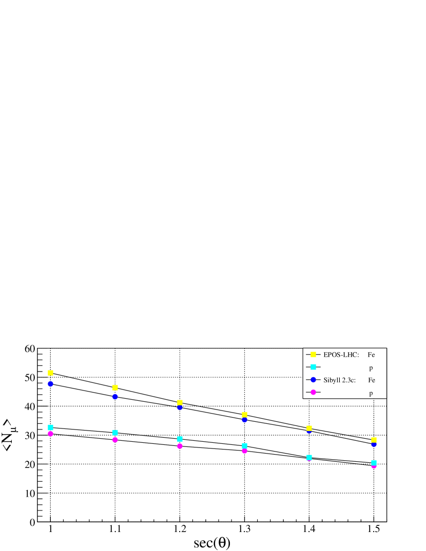
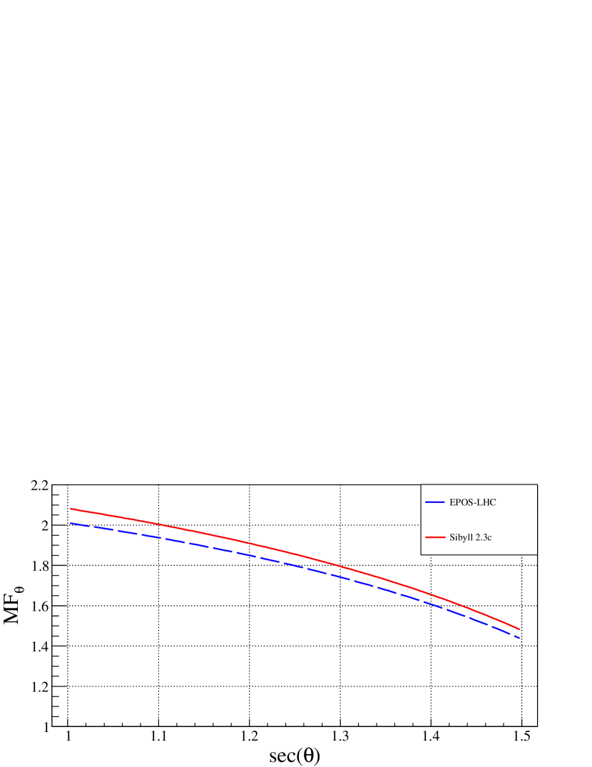
Figure 1: Top: $\langle N_{\mu}\rangle$ as a function of sec$(\theta)$ for $E=10^{18}$ eV corresponding to proton ($p$) and iron ($Fe$) primaries. The error bars are smaller than the marker size. Bottom: Merit factor of $\widetilde{N}_{\mu}$ as a function of $\sec(\theta)$. The two HEHIMs considered are EPOS-LHC and Sibyll 2.3c.

As mentioned above, the distribution function of $N_{\mu}$ presents asymmetric tails. However, the distribution function of the reconstructed $N_{\mu}$, i.e. $\widetilde{N}_{\mu}$, is given by the convolution of the distribution function of $N_{\mu}$ with the one that takes into account the fluctuations introduced by the detectors and the effects of the reconstruction methods. As a result, a Gaussian distribution is a good approximation of the distribution function corresponding to the reconstructed number of muons Supa:15 , which is given by,

$$P^{\theta}_{A}(\widetilde{N}_{\mu}|E)=\frac{1}{\sqrt{2\pi}\ \sigma[\widetilde{N}_{\mu}]^{\theta,E}_{A}}\exp\left[-\frac{\left(\widetilde{N}_{\mu}-\langle N_{\mu}\rangle^{\theta,E}_{A}\right)^{2}}{2\ \sigma^{2}[\widetilde{N}_{\mu}]^{\theta,E}_{A}}\right],$$ (5)

where $\sigma[\widetilde{N}_{\mu}]^{\theta,E}_{A}\equiv\sigma[\widetilde{N}_{\mu}](E,\textrm{sec}(\theta),A)$ is given by,

$$\sigma^{2}[\widetilde{N}_{\mu}]^{\theta,E}_{A} = \sigma_{sh}^{2}[N_{\mu}]^{\theta,E}_{A}\left(\sigma^{2}[\epsilon]^{\theta,E}_{A}+1\right)$$ (6)

$$+\sigma^{2}[\epsilon]^{\theta,E}_{A}\left[\langle N_{\mu}\rangle^{\theta,E}_{A}\right]^{2}.$$

Here $\sigma[\epsilon]^{\theta,E}_{A}\equiv\sigma[\epsilon](E,\sec(\theta),A)$ is the relative error of the reconstructed number of muons, i.e. $\sigma[\epsilon]=\sigma[\widetilde{N}_{\mu}/\langle N_{\mu}\rangle-1]$.

In Ref. Supa:15 $\sigma[\epsilon]$ at 750 m from the shower axis is calculated from simulations of the showers and the AMIGA detectors by using the reconstruction method of the muon lateral distribution function developed in that work. In that calculation the core position and the arrival direction of the showers are reconstructed by using the information of the water Cherenkov detectors whereas the muon lateral distribution function is reconstructed by using the information given by the muon counters but using the core position determined with the Cherenkov detectors. The values of $\sigma[\epsilon]$ used in this work are obtained by fitting the data points shown in Fig. 9 (right panel) of Ref. Supa:15 between $10^{17.6}$ and $10^{18.5}$ eV, for proton and iron primaries and for $\theta=45^{\circ}$. The proton data points are fitted with a cubic function of $\log(E/\textrm{eV})$ with coefficients: $a_{0}=1163.0$, $a_{1}=-190.199$, $a_{2}=10.3725$ and $a_{3}=-0.188612$. The iron data points are fitted with a quadratic function of $\log(E/\textrm{eV})$ with coefficients: $b_{0}=21.2686$, $b_{1}=-2.27008$ and $b_{2}=0.0607638$. Note that $a_{i}$ and $b_{i}$ are the coefficients of the $i$th power of $\log(E/\textrm{eV})$. Fig. 2 shows the fitted $\sigma[\epsilon]$ as a function of $\log(E/\textrm{eV})$ for proton and iron primaries. Although $\sigma[\epsilon]$ is nearly independent of zenith angle, the $\theta=45^{\circ}$ data points are considered due to their slightly larger values compared with the ones obtained for $\theta=30^{\circ}$ (see Fig. 9 of Ref. Supa:15 ). Also, $\sigma[\epsilon]$ at 750 m from the shower axis is used for $\sigma[\epsilon]$ at 450 m, this is an approximation based on the results obtained in Ref. Ravignani:15 in which it is shown that a similar or even smaller value of $\sigma[\epsilon]$ is obtained at 450 m from the shower axis considering an improved reconstruction method developed in that work. Therefore, the values of $\sigma[\epsilon]$ used for the present calculations include the effects introduced by the detectors and the reconstruction methods conservatively.

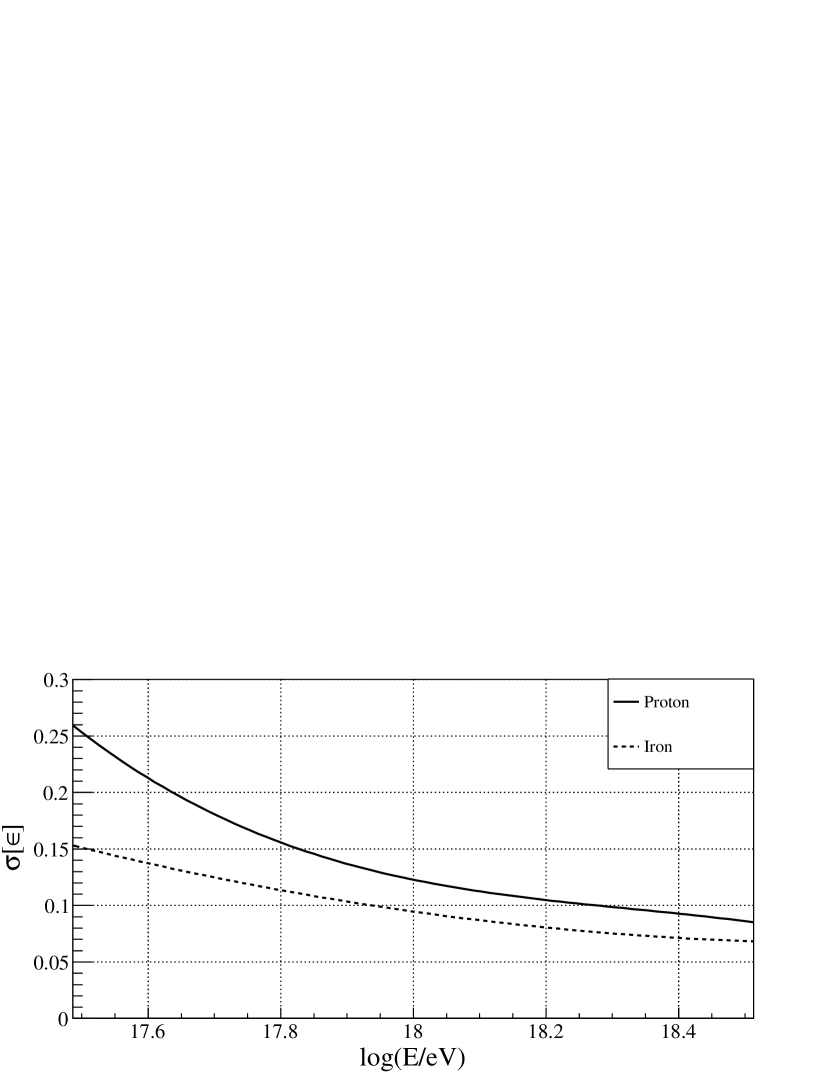
Figure 2: Relative error corresponding to the reconstructed number of muons as a function of the logarithm of the energy for proton and iron nuclei and zenith angle $\theta=45^{\circ}$.

$\langle N_{\mu}\rangle^{\theta,E}_{A}$ and $\sigma_{sh}[N_{\mu}]^{\theta,E}_{A}$ are obtained from the CORSIKA simulations. For each primary type and HEHIM both quantities are obtained by fitting the simulated data with linear functions of $\sec(\theta)$ such that the coefficients are cubic functions of $\log(E/\textrm{eV})$.

The discrimination power of a given mass sensitive parameter, $q$, can be assessed by the commonly used merit factor, which is defined as,

$$\textrm{MF}(q)=\frac{\langle q\rangle_{A_{2}}-\langle q\rangle_{A_{1}}}{\sqrt{\textrm{Var}[q]_{A_{2}}+\textrm{Var}[q]_{A_{1}}}},$$ (7)

where $\textrm{Var}[q]_{A}$ is the variance of parameter $q$ for the primary type $A$. The bottom panel of Fig. 1 shows the $\textrm{MF}(\widetilde{N}_{\mu})$ as a function of $\sec(\theta)$ (denoted in this work as $\textrm{MF}_{\theta}$) for the two HEHIMs. It can be seen that the curves present similar $\textrm{MF}_{\theta}$ due to the small differences between the number of muons predicted by the two different HEHIMs considered. It can also be seen that the curves have $\textrm{MF}_{\theta}$ values compatible with those found in Ref. Supa:08 reaffirming that the muon content of the showers is the best indicator of primary mass composition together with $X_{max}$ Kamp:12 ; Supa:08 .

The energy range considered in this work ranges from $10^{17.5}$ to $10^{18.5}$ eV, which corresponds to the 750 m array of AMIGA. In this energy range the cosmic ray flux can be approximated as $J(E)=C\,E^{-3.27}$ Verzi:19 where $C$ is a normalization constant. The conditional probability distribution $G(E_{R}|E)$ is assumed to be a Gaussian distribution,

$$G(E_{R}|E)=\frac{1}{\sqrt{2\pi}\ \sigma[E]}\exp\left[-\frac{(E_{R}-E)^{2}}{2\ \sigma^{2}[E]}\right],$$ (8)

where $\sigma[E]=(0.084+0.047\sqrt{10^{18}\,\textrm{eV}/E})\times E$ is the surface detectors energy resolution corresponding to Auger in the energy range under consideration Cole:19 . Then, by using Eq. (8) it is possible to express Eq. (2) as follows,

$$P^{\theta}_{A}(\widetilde{N}_{\mu}|E_{Ri})=\frac{\displaystyle\int_{0}^{\infty}\!\!\!I(E,E_{Ri}^{+},E_{Ri}^{-})\,J(E)\,P^{\theta}_{A}(\widetilde{N}_{\mu}|E)\,dE}{\displaystyle\int_{0}^{\infty}\!\!\!I(E,E_{Ri}^{+},E_{Ri}^{-})\,J(E)\,dE},$$ (9)

where

$$I(E,E_{Ri}^{+},E_{Ri}^{-})=\frac{1}{2}\left[\text{erf}\left(\frac{E_{Ri}^{+}-E}{\sqrt{2}\,\sigma[E]}\right)-\text{erf}\left(\frac{E_{Ri}^{-}-E}{\sqrt{2}\,\sigma[E]}\right)\right],$$ (10)

being $\text{erf}(x)$ the error function. Reconstructed energy bins of width $\log(E_{Ri}^{+}/\textrm{eV})-\log(E_{Ri}^{-}/\textrm{eV})=0.1$ centered at $E_{Ri}$ are considered. Finally, it is worth mentioning that the integrals of Eq. (9) are solved numerically.

II.3 Simulations for the study of the proton abundance estimator

The simulations for the study of the performance of $\hat{c}_{p}$, the estimator of the proton abundance ($A_{1}=p$), $c_{p}$, are performed by using the ROOT package Root . The values of $c_{p}$ considered range between $0.1$ and $0.9$ in steps of $0.1$. Given the $i$-th reconstructed energy bin, for each value of $c_{p}$, the number of events, $N_{p}$, due to proton induced air showers is obtained by sampling a Binomial distribution function, $B(N,c_{p})$, where $N$ is the total number of events in the $i$-th bin. $N$ is obtained by sampling a Poisson distribution with mean value given by,

$$\mu_{i}=T\,A_{c}\,\int_{E_{Ri}^{-}}^{E_{Ri}^{+}}J(E)dE$$ (11)

where $T$ is the observation time considered (5 and 10 years) and $A_{c}$ is the acceptance of the detector. The zenith angle interval from 0 to $45^{\circ}$ is considered (the one corresponding to the AMIGA muon detectors), then, $A_{c}=S\,\pi\sin^{2}(45^{\circ})$ where $S=25$ $\textrm{km}^{2}$ is approximately the area of the 750 m AMIGA array. The number of events due to the other primary $A_{2}$ ($Iron$ or $Nitrogen$) is calculated as $N_{A_{2}}=N-N_{p}$.

The simulated energy $E_{j}$ of an event that belongs to the $i$-th bin is obtained by sampling the flux $J(E)$ (adequately normalized) in a wide energy interval centered at $E_{Ri}$. The reconstructed energy $E_{R,j}$ is obtained by sampling the Gaussian distribution of Eq. (8) centered at $E_{j}$. This sampling process is repeated until the reconstructed energy $E_{R,j}$ falls in the $i$-th reconstructed energy bin. The zenith angle corresponding to each event is taken at random from an isotropic distribution ($f(\theta)\propto\sin(\theta)\cos(\theta)$) in the zenith angle range mentioned before. The parameter $\widetilde{N}_{\mu}$ for each event is obtained by sampling a Gaussian distribution (see Eq. (5)) obtained evaluating the mean value and the standard deviation, corresponding to the primary type of the event, in the zenith angle and simulated energy obtained before.

For each value of $c_{p}$, $10^{3}$ independent samples are generated in order to obtain the distribution function of $\hat{c}_{p}$. The mean value of the proton abundance estimator, $\langle\hat{c}_{p}\rangle$, and its standard deviation, $\sigma_{\hat{c}_{p}}$ are calculated.

In order to analyze the impact of the differences between HEHIMs on composition analyses a given HEHIM, called the reference model, is used to generate the event samples, which is not necessarily the same as the one used to analyze the data, i.e. to calculate the parameters of the Gaussian distributions involved in the calculation of $\hat{c}_{p}$ by means of Eq. (4).

We consider the HEHIMs Sibyll 2.3c, EPOS-LHC, and *Sibyll 2.3c, a modified version of Sibyll 2.3c for which the values of $\langle N_{\mu}\rangle^{\theta,E}_{A}$ and $\sigma[\widetilde{N}_{\mu}]^{\theta,E}_{A}$ are obtained by multiplying the ones corresponding to Sibyll 2.3c by a factor (1 + $\varepsilon$) with $\varepsilon=\textrm{constant}$. Note that *Sibyll 2.3c is constructed in such a way that the parameter $N_{\mu}$ has the same merit factor as the one obtained for Sibyll 2.3c, regardless the pair of primary types considered.

In order to analyze the results obtained from the simulations the following quantities are considered: The bias of $\hat{c}_{p}$, which is given by,

$$\delta_{c_{p}}=\langle\hat{c}_{p}\rangle(\textrm{HM},\textrm{HM}_{ref})-c_{p},$$ (12)

and the percentage difference, $\Delta\sigma_{c_{p}}$, which is defined as,

$$\Delta\sigma_{c_{p}}=100\%\ \left[\frac{\sigma_{\hat{c}_{p}}(\textrm{HM},\textrm{HM}_{ref})}{\sigma_{\hat{c}_{p}}(\textrm{HM}_{ref},\textrm{HM}_{ref})}-1\right],$$ (13)

where $\langle\hat{c}_{p}\rangle(\textrm{HM},\textrm{HM}_{ref})$ and $\sigma_{\hat{c}_{p}}(\textrm{HM},\textrm{HM}_{ref})$ are the mean value and the standard deviation of the estimator $\hat{c}_{p}$, respectively, $\textrm{HM}_{ref}$ is the reference model considered, and HM is the HEHIM used to analyze the simulated data.

III Results and Discussion

III.1 Performance of the Maximum Likelihood method

Figure 3 shows $\delta_{c_{p}}$ (top) and $\sigma_{\hat{c}_{p}}$ (bottom) as a function of $c_{p}$ calculated with the ML method for Sibyll 2.3c and EPOS-LHC used each one of those as the reference model and to analyze the data (HM = HM_ref), $E_{Ri}=10^{18}$ eV and random sample size $N$ corresponding to 5 and 10 years of collected events at AMIGA 750 m array ($N\sim 10^{3}$ for 5 years). From Fig. 3 (top) one can see that the bias is negligible over the entire $c_{p}$ range for both HEHIMs considered. It is worth mentioning that in previous studies done for fixed values of the zenith angle the biases obtained are also negligible in the entire zenith angle range considered. From the $\sigma_{\hat{c}_{p}}$ values of Fig. 3 (bottom) it can also be seen that proton abundance is estimated with high resolution showing that the muon content of the shower is one of the best indicators of primary mass composition. Fig. 3 (bottom) also shows that the differences between the values of $\sigma_{\hat{c}_{p}}$ obtained with Sibyll 2.3c and EPOS-LHC are less than $10\%$ due to the similarity of their $\textrm{MF}_{\theta}$ (Fig. 1 bottom). From the figure it can also be seen that $\sigma_{\hat{c}_{p}}$ has a maximum around $c_{p}=0.5$ and that it is smaller for $c_{p}=0.1$ than for $c_{p}=0.9$. The maximum at $c_{p}\cong 0.5$ can be understood from the fact that at $c_{p}=0.5$ the fluctuations on the number of proton events only and in the number of iron events only are the largest (from the expression of the standard deviation of a binomial variable it can be seen that $\sigma[N_{p}]=\sigma[N_{Fe}]=\sqrt{N}/2$) causing the appearance of the maximum. For values of $c_{p}$ close to zero the number of iron events increases and its fluctuations decrease ($\sigma[N_{Fe}]=\sqrt{Nc_{p}(1-c_{p})}$) causing the decrease of the uncertainty on the determination of $c_{p}$. The same happens for values of $c_{p}$ close to one. The larger values of $\sigma_{\hat{c}_{p}}$ obtained at $c_{p}=0.9$ compared with the ones obtained for $c_{p}=0.1$ has to do with the fact that the width of the $\widetilde{N}_{\mu}$ proton distribution is larger than the one corresponding to iron.

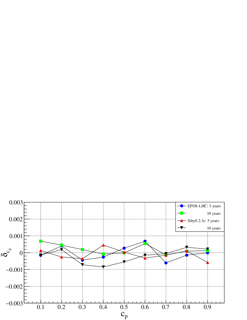
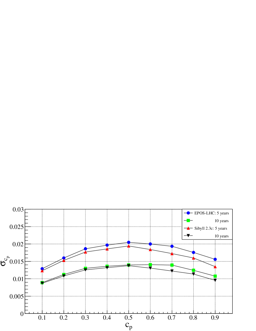
Figure 3: $\delta_{c_{p}}$ (top) and $\sigma_{\hat{c}_{p}}$ (bottom) versus $c_{p}$ calculated with the ML method for $E_{Ri}=10^{18}$ eV, sample size $N$ corresponding to 5 and 10 years of observation, and for binary mixtures of proton and iron primaries. The HEHIMs used are Sibyll 2.3c and EPOS-LHC. In both cases the reference model is also used to analyze the data, i.e.  HM=HM_ref.

Hereafter only Sibyll 2.3c will be considered as the reference model, i.e. HM_ref = Sibyll 2.3c. Fig. 4 shows $\delta_{c_{p}}$ (top) and $\Delta\sigma_{c_{p}}$ (bottom) for different values of $\varepsilon$ (see section II.3), i.e. HM = *Sibyll 2.3c. The case corresponding to HM = EPOS-LHC is also shown in the figure. All cases correspond to $E_{Ri}=10^{18}$ eV and $N$ for 5 years of observation. Note that $\varepsilon=0$ corresponds to the case in which HM = HM _ref, then $\Delta\sigma_{c_{p}}(\varepsilon=0)=0$ by definition and $\delta_{c_{p}}(\varepsilon=0)=0$ since the ML method does not produce bias. Note also that $\delta_{c_{p}}$ is greater than zero since $\varepsilon>0$. The same applies for the case of EPOS-LHC whose $\langle N_{\mu}\rangle$ values are greater than those of Sibyll 2.3c (Fig. 1 top).

From Fig. 4 it can also be seen that as $\varepsilon$ approaches zero, the curve $\delta_{c_{p}}$ ($\Delta\sigma_{c_{p}}$) becomes more symmetric (antisymmetric) around $c_{p}=0.5$. The same can be said for $\varepsilon<0$ cases (not shown in the figure) since $\delta_{c_{p}}(\varepsilon)=-\delta_{c_{p}}(-\varepsilon)$ and $\Delta\sigma_{c_{p}}(\varepsilon)=-\Delta\sigma_{c_{p}}(-\varepsilon)$ when $|\varepsilon|\ll 1$.

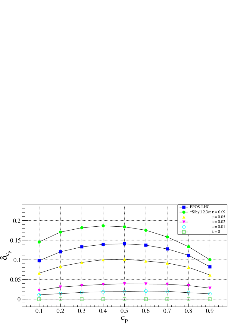
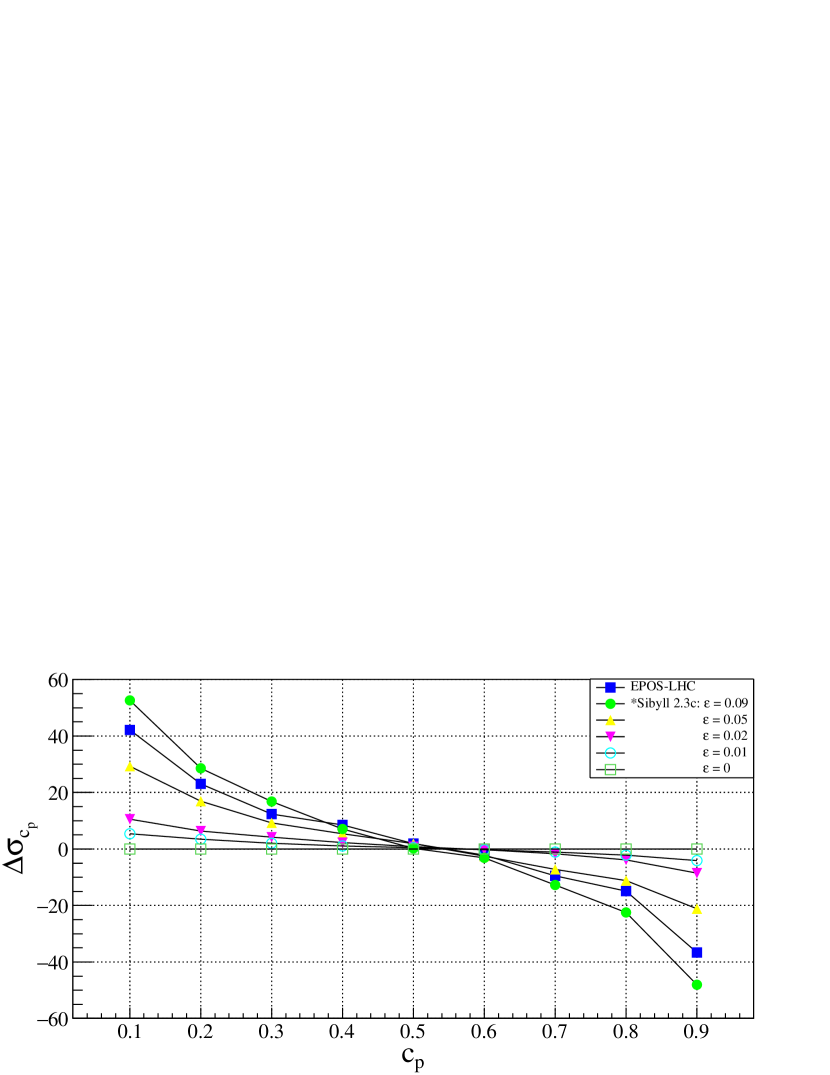
Figure 4: $\delta_{c_{p}}$ (top) and $\Delta\sigma_{c_{p}}$ (bottom) versus $c_{p}$ for the ML method and for different values of $\varepsilon$ (see section II.3). The case corresponding to HM=EPOS-LHC is also shown. All cases correspond to $E_{Ri}=10^{18}$ eV, binary mixtures of proton and iron primaries, and sample size for 5 years of observation.

The small differences between the number of muons at ground predicted by post-LHC HEHIMs and therefore, between their $\textrm{MF}_{\theta}$, allows us to use any of them as a reference, obtaining similar absolute values of $\delta_{c_{p}}$ and $\Delta\sigma_{c_{p}}$. From the figure it can also be seen that $|\delta_{c_{p}}|$ and $|\Delta\sigma_{c_{p}}|$ increase strongly with $\varepsilon$, indicating that slight differences between the number of muons predicted by different HEHIMs have a significant impact on composition determination (see for instance Prado:16 ).

It is worth mentioning that the values of $\delta_{c_{p}}$, $\sigma_{\hat{c}_{p}}$ and $\Delta\sigma_{c_{p}}$ depend on the statistical method used to estimate $c_{p}$. However, impacts of the same order are expected for other methods that make use of the number of muons as a mass sensitive parameter. As an example, let us consider the case in which the sample mean of the measured $\widetilde{N}_{\mu}$ is used to estimate $c_{p}$. To simplify the calculation let us assume that the energy uncertainty is negligible. Under this assumption the following expression for the bias, at order one in $\varepsilon$, is obtained,

$$\delta_{c_{p}}\cong\varepsilon\left[\frac{\langle\widetilde{N}_{\mu}\rangle_{Fe}}{\langle\widetilde{N}_{\mu}\rangle_{Fe}-\langle\widetilde{N}_{\mu}\rangle_{p}}-c_{p}\right]$$ (14)

where $\langle\widetilde{N}_{\mu}\rangle_{p}$ and $\langle\widetilde{N}_{\mu}\rangle_{Fe}$ are the mean values of $\widetilde{N}_{\mu}$ corresponding to proton and Iron primaries for the reference model. Assuming that $\langle\widetilde{N}_{\mu}\rangle_{p}=27$ and $\langle\widetilde{N}_{\mu}\rangle_{Fe}=42$, the values obtained for Sibyll 2.3c at $\theta=30^{\circ}$, the median of the $\sin(\theta)\cos(\theta)$ distribution for $\theta\in[0^{\circ},45^{\circ}]$ (see Fig. 1), the bias obtained for $\varepsilon=0.09$ decrease from $\sim 0.25$ at $c_{p}=0$ to $\sim 0.16$ at $c_{p}=1$, which is even larger than the one obtained for the ML method.

III.2 Current and future HEHIMs features

An analysis performed by the Pierre Auger Observatory indicates that, in the best case, the number of muons measured in the energy range from $10^{18.8}$ to $10^{19.2}$ eV and for $0-60^{\circ}$ inclined showers differs from HEHIMs predictions by a factor $R=1.33\pm 0.16$ Aab:16 . At lower energies, between $10^{17.5}$ and $10^{18}$ eV, the AMIGA data show a muon deficit in simulations of $38\%$ for EPOS-LHC and $50-53\%$ for QGSJETII-04 Muller:18 . This deficit in the muon content of the showers has been observed also by other experiments in different energy ranges (see Ref. Dembinski:19 and references there in). The experimental data show that this deficit increases with primary energy. It is not yet known whether this discrepancy in the number of muons could be indicative of the beginning of some new phenomenon in hadronic interactions at ultra high energies Farrar:13 ; Alvarez:13 or can be explained by some incorrectly modeled features of hadronic interactions even at low energy Dres:04 ; Maris:09 , as for example, baryon-antibaryon pair production Pierog:08 ; Pierog:13 or resonance mesons Dres:08 .

The experimental data also show that the muon deficit observed increases with $\sec(\theta)$. This behavior is observed at low energies (between $10^{16.3}$ and $10^{17}$ eV) by the KASCADE-Grande Collaboration Kascade and at higher energies (between $10^{18.8}$ and $10^{19.2}$ eV) by Auger Aab:16 . This behavior can be partially explained by the fact that the experimental value of the attenuation length of the number of muons in the atmosphere is greater than the values obtained from Monte Carlo simulations of the showers Kascade . This implies that the observed air showers attenuate more slowly in the atmosphere than the simulated ones. The disagreement on the attenuation length between Monte Carlo predictions and the experimental measurements most likely originates from muon prediction deficiencies of the HEHIMs Kascade . The uncertainty in the shape of the muon lateral distribution function employed to reconstruct the EAS data also contributes to this discrepancy, but it is not the principal effect Kascade .

The produced number of muons increases with a small power of the mass number and almost linearly with the primary energy. This behavior can be understood in terms of the Heitler-Matthews model of hadronic air showers Matthews:05 , which predicts that the mean value of the total number of muons produced in a shower is $\langle N_{\mu}^{T}\rangle(E,A)=A\left[E/(A\ \xi_{c})\right]^{\beta}$, where $\xi_{c}$ is the critical energy at which charged pions decay into muons. Simulations with post-LHC HEHIMs show that $\beta\simeq 0.915-0.928$ Pierog:17 ; Prado:16 . Note from Fig. 1 (top) that the ratio $\langle N_{\mu}\rangle^{\theta,E}_{Fe}/\langle N_{\mu}\rangle^{\theta,E}_{p}$, evaluated at $E_{0}=10^{18}$ eV, is greater than $\left(56/1\right)^{1-\beta}$. This increment occurs because the energy spectrum of muons is harder for iron showers than for proton ones Espadanal:16 . In the same way, since the muon counters are buried underground, the soil attenuates in a greater proportion the muons from proton primaries. Although there is still a large uncertainty related to the energy spectrum of the produced muons Pierog:17 , in Ref. Espadanal:16 it was found that by changing the energy spectrum by an amount consistent with the difference between current HEHIMs, the number of muons at ground for the same $\sec(\theta)$ changes by the same factor for all primaries and hadronic models. This factor increases (decreases) with $\sec(\theta)$ if the muon energy spectrum is hardened (softened). This behavior occurs because at larger zenith angles, muons travel, on average, larger distances before reaching ground, making the decay of low energy muons more important Espadanal:16 .

On the other hand, the number of muons can change under variation of several important features of the hadronic interactions i.e., hadronic particle production cross sections, multiplicity, elasticity and, in particular, pion charge-ratio Ulrich:11 . Fluctuations in the number of muons can also change under a modification of these interaction features, being especially sensitive to elasticity Ulrich:11 . The Pierre Auger Observatory also found no evidence of a larger event-to-event variance in the ground signal for fixed $X_{max}$ than the one predicted by current HEHIMs Aab:16 . This suggests that the muon deficit cannot be attributed to an exotic phenomenon producing a very large muon signal in a fraction of events only Aab:16 , such as a high rate production of microscopic black holes Feng:02 .

It is expected that the observed muon deficit can be reduced in the next generation of HEHIMs, at least for $0-60^{\circ}$ inclined showers Pierog:17 . Therefore, assuming that the current mean values $\langle N_{\mu}\rangle^{\theta,E}_{A}$ will be increased by some factor, $R(E,\sec(\theta))$ (almost independent of $A$), the difference $\langle N_{\mu}\rangle^{\theta,E}_{A_{2}}-\langle N_{\mu}\rangle^{\theta,E}_{A_{1}}$ will be increased by the same factor. Although it is not possible to know whether $\sigma_{sh}[N_{\mu}]^{\theta,E}_{A}$ will increase, decrease or remain unchanged, $\sigma[\widetilde{N}_{\mu}]^{\theta,E}_{A}$ will increase because it is dominated by $\langle N_{\mu}\rangle^{\theta,E}_{A}$ (see Eq. (6)). Then, the $\textrm{MF}_{\theta}$ will suffer only a slight modification, having a similar impact on composition determination under the same relative differences between HEHIMs, or eventually, between a given HEHIM and the experimental data. Fig. 5 shows $\delta_{c_{p}}$ (top) and $\Delta\sigma_{c_{p}}$ (bottom) for the same cases of Fig. 4 but with the $\langle N_{\mu}\rangle^{\theta,E}_{A}$ values multiplied by a hypothetical (naive) factor $R(E,\sec(\theta))=1.4$. In the same way Fig. 6 shows $\delta_{c_{p}}$ (top) and $\Delta\sigma_{c_{p}}$ (bottom) for the same cases of Fig. 5 with $R(E,\sec(\theta))=1.4$ but with the $\sigma_{sh}[N_{\mu}]^{\theta,E}_{A}$ values multiplied by a factor 2. It can be seen that $|\delta_{c_{p}}|$ and $|\Delta\sigma_{c_{p}}|$ of Figs. 5 and 6 are similar to the ones corresponding to Fig. 4. Therefore, these results suggest that future HEHIMs will have a similar impact on composition determination than current ones.

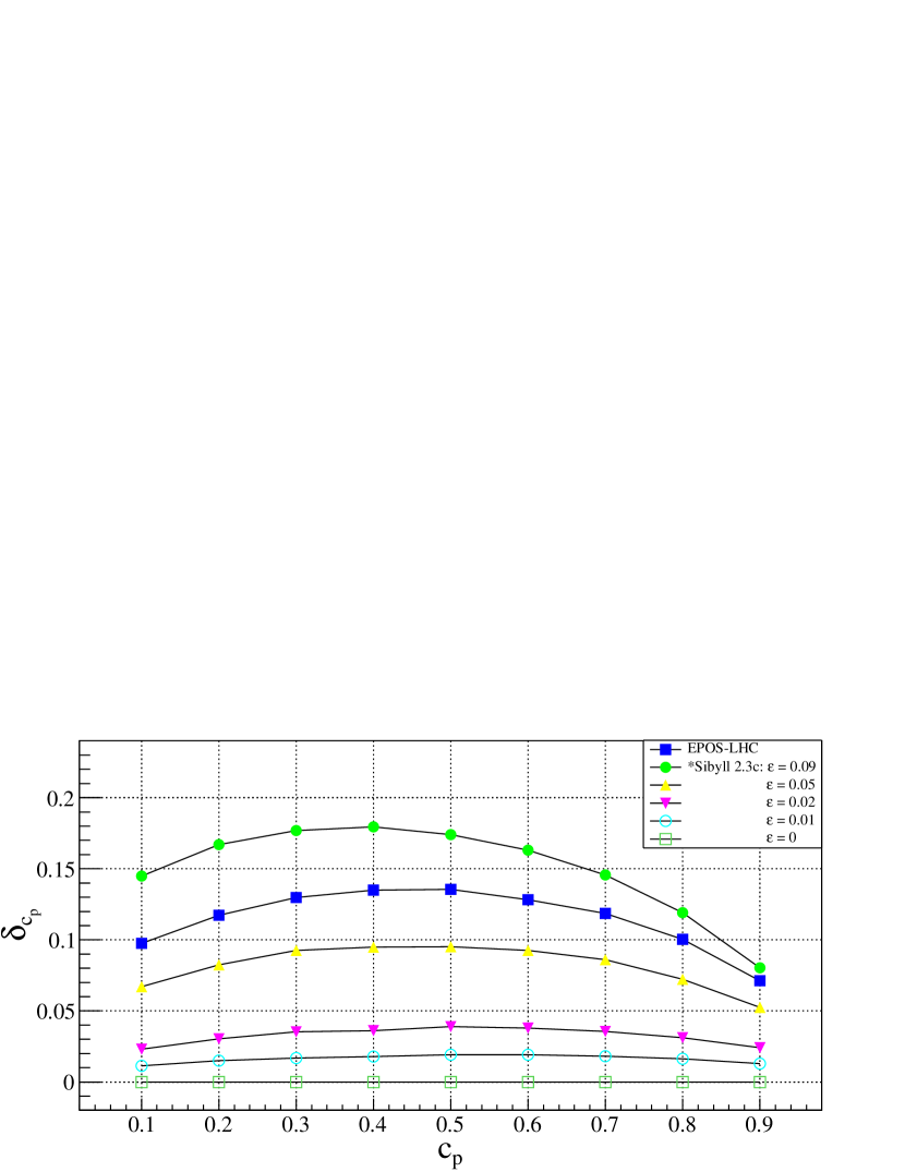
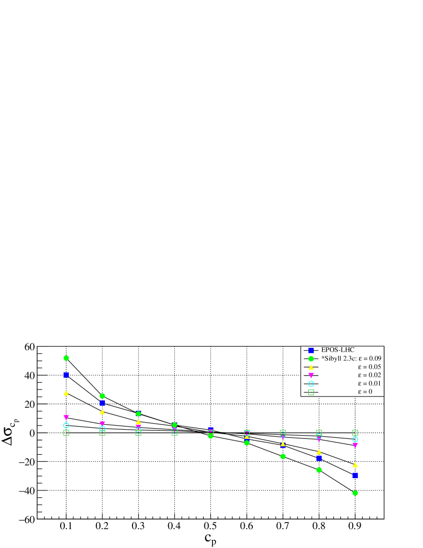
Figure 5: $\delta_{c_{p}}$ (top) and $\Delta\sigma_{c_{p}}$ (bottom) versus $c_{p}$ for the ML method and for different values of $\varepsilon$ (see section II.3). The case corresponding to HM=EPOS-LHC is also shown. All cases correspond to $E_{Ri}=10^{18}$ eV, sample size for 5 years of observation, and $R(E,\sec(\theta))=1.4$.

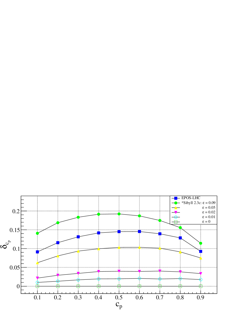
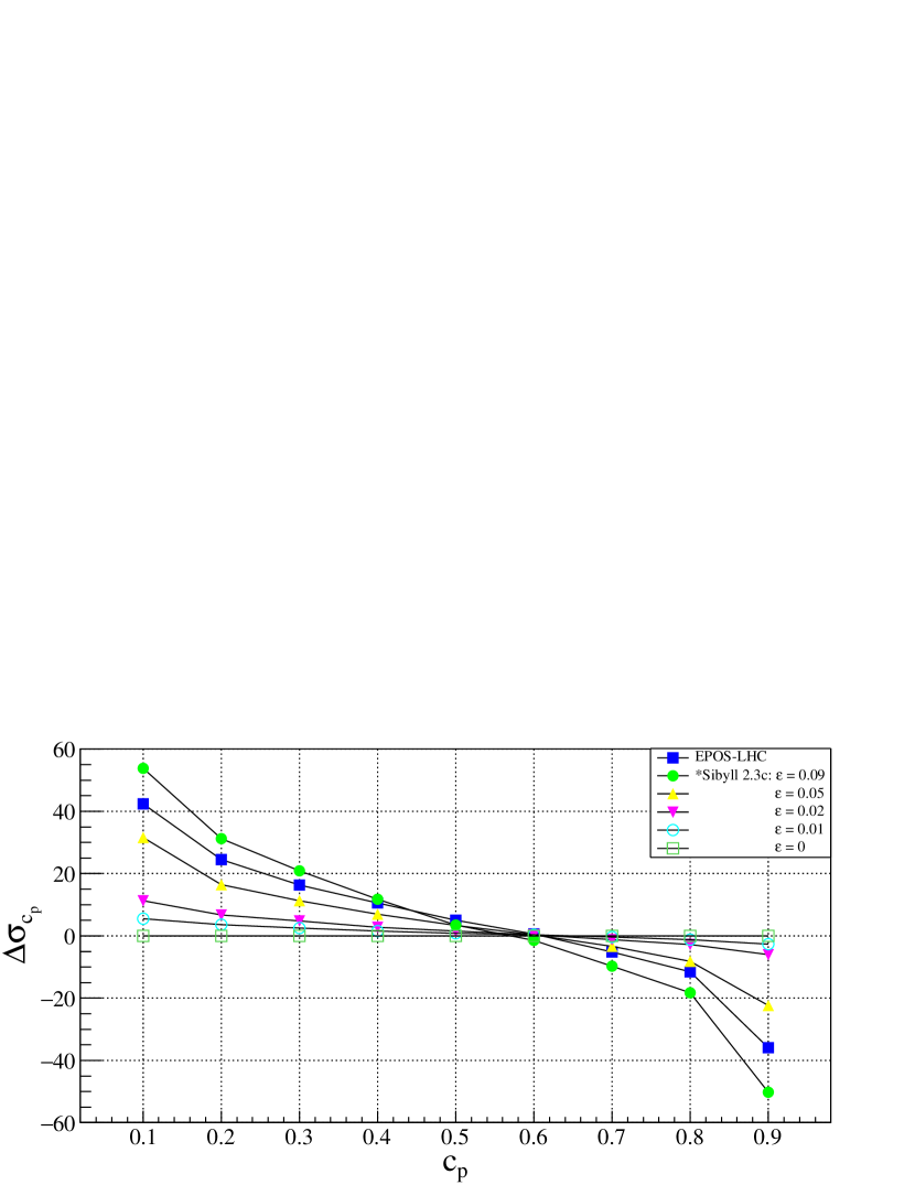
Figure 6: $\delta_{c_{p}}$ (top) and $\Delta\sigma_{c_{p}}$ (bottom) versus $c_{p}$ for the ML method and for different values of $\varepsilon$ (see section II.3). The case corresponding to HM=EPOS-LHC is also shown. All cases correspond to $R(E,\sec(\theta))=1.4$, but with the $\sigma_{sh}[N_{\mu}]^{\theta,E}_{A}$ values multiplied by a factor 2 (for both, Sibyll 2.3c and EPOS-LHC).

III.3 Application to a simplified case

In this section the impact of the HEHIMs in composition analyses is studied in the energy range from $10^{17.5}$ and $10^{18.5}$ eV, assuming a binary mixture of protons and nitrogen nuclei. This assumption is based on the results obtained in Ref. Bellido . In that work a sample of 42466 events recorded by the Pierre Auger Observatory is used to obtain the $X_{max}$ distributions in energy bins of $\Delta\log(E/\textrm{eV})=0.1$, ranging from $10^{17.2}$ eV to $10^{19.6}$ eV. The experimental distributions are fitted considering the $X_{max}$ distributions obtained for Sibyll 2.3c, EPOS-LHC, and QGSJETII-04, including the detector effects. The composition fractions are estimated assuming four elemental primary groups: proton, helium, nitrogen, and iron. In the energy range from $10^{17.5}$ to $10^{18.5}$ eV protons and nitrogen nuclei turn out to be the most abundant nuclear species when Sibyll 2.3c is considered to analyze the $X_{max}$ Auger data. Note that the fraction of helium is also appreciable for energies greater than $10^{18}$ eV but with large error bars.

The top panel of Fig. 7 shows the inferred $\hat{c}_{p}$ values with their statistical uncertainties for sample size $N$ corresponding to 5 years of observation and Sibyll 2.3c as the reference HEHIM, obtained for different values of $\varepsilon$ in the energy range under consideration. The relative error of the reconstructed number of muons, $\sigma[\epsilon]$, used for nitrogen is approximated by the average between the ones corresponding to proton and iron primaries. The values of $c_{p}(E_{Ri})$ considered as input are extracted from the Fig. 6 of Ref. Bellido . The error bars correspond to $\sigma_{\hat{c}_{p}}$. Note that $\delta_{c_{p}}(E_{Ri}=10^{18}\ \textrm{eV},\varepsilon)$ are larger than those of Fig. 4 (top), this is due to the fact that the merit factor for proton and nitrogen is smaller than the one corresponding to proton and iron.

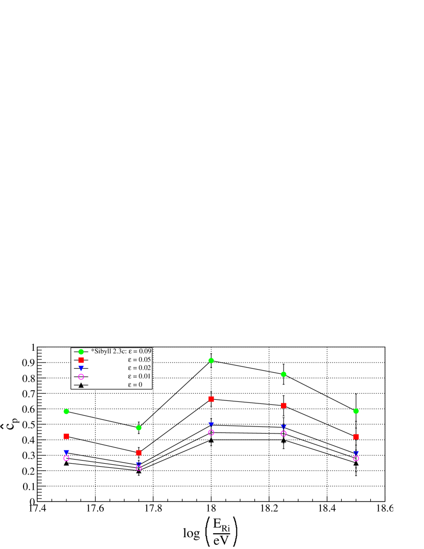
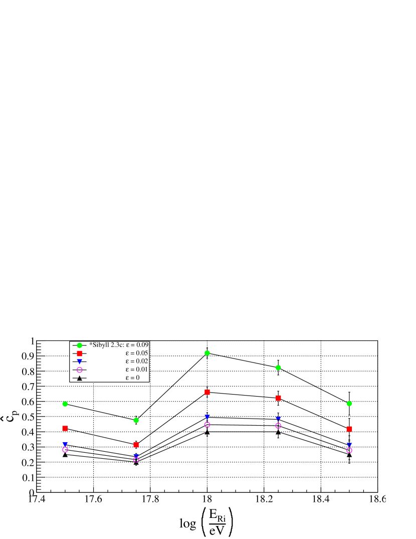
Figure 7: $\hat{c}_{p}$ as a function of $E_{Ri}$ for different values of $\varepsilon$ (see section II.3) and sample size corresponding to 5 (top) and 10 (bottom) years of observation. The error bars correspond to $\sigma_{\hat{c}_{p}}$. $\sigma[\epsilon]$ for nitrogen is approximated by the average between the ones corresponding to proton and iron primaries.

The bottom panel of Fig. 7 shows the $\hat{c}_{p}$ values for the same case shown at the top one but for sample size $N$ corresponding to 10 years of observation. As expected, the error bars of the reconstructed $c_{p}$ are smaller than those at the top panel.

Figure 8 shows the inferred $\hat{c}_{p}$ values for the same cases as in Fig. 7 but using the same $\sigma[\epsilon]$ for nitrogen as for proton (conservative case). As expected, the biases and the error bars in Fig. 8 are larger than those of Fig. 7 (especially for $\varepsilon\gtrsim 0.05$). However, they are very similar for energies $\geq 10^{18}$ eV. This can be explained from Fig. 2 where it is seen that for energies above $10^{18}$ eV $\sigma[\epsilon]$ of protons is larger than $\sigma[\epsilon]$ of iron nuclei in less than 3%.

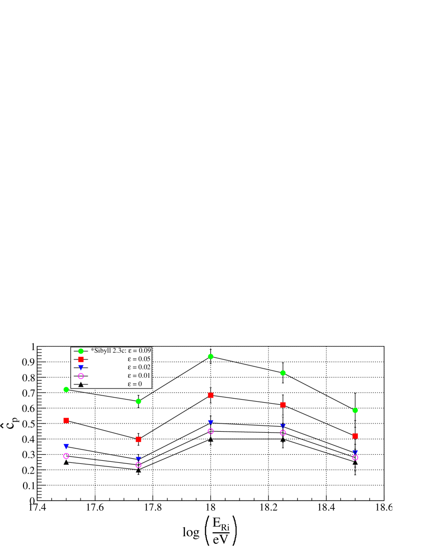
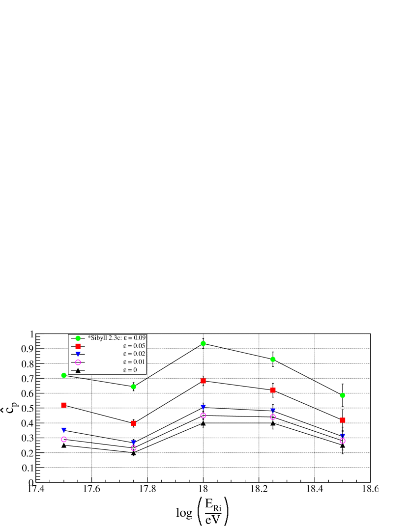
Figure 8: $\hat{c}_{p}$ as a function of $E_{Ri}$ for different values of $\varepsilon$ (see section II.3) and sample size corresponding to 5 (top) and 10 (bottom) years of observation. The error bars correspond to $\sigma_{\hat{c}_{p}}$. $\sigma[\epsilon]$ used for nitrogen is the same as the one obtained for proton primaries (conservative case).

From Figs. 7 and 8 it can also be seen that to ensure $|\delta_{c_{p}}|\lesssim 0.05$, the differences between $\langle N_{\mu}\rangle^{\theta,E}_{A}$ of different HEHIMs must be smaller than $2\%$. It is well known that the mass composition determination obtained from the $X_{max}$ parameter also depends on the HEHIMs used in the analyses Bellido ; Abreu:13 ; Aab:14 . Comparing the results obtained in this work with the ones obtained in Ref. Bellido at $E_{Ri}=10^{18}$ eV (energy at which the mass composition obtained by using $X_{max}$ corresponds basically to a binary mixture of protons and nitrogen nuclei), it can be seen that $\delta_{c_{p}}(E_{Ri}=10^{18}\ \textrm{eV},\varepsilon=0.05)$ is of the order of the bias found in the analysis based on the $X_{max}$ parameter when Sibyll 2.3c and EPOS-LHC are used to estimate the proton abundance. Therefore, it indicates that the systematic uncertainties introduced by the use of different HEHIMs on composition analyses based on the $N_{\mu}$ parameter are of the same order as the ones based on the $X_{max}$ parameter.

In summary it is found that small differences between the predicted values of $\langle N_{\mu}\rangle^{\theta,E}_{A}$ and $\sigma_{sh}[N_{\mu}]^{\theta,E}_{A}$ obtained when different HEHIMs are considered have a significant impact on composition determination. It is worth mentioning that in recent years different mass composition methods that seem to have a reduced dependence on the assumed HEHIM have been developed. In Ref. Blaess:18 a method of this type, which is based on the $X_{max}$ distributions, is presented. This method is based on parametrizations of the $X_{max}$ distributions obtained from simulations in which the normalization levels of the mean value and the standard deviation of $X_{max}$ are determined from experimental data. In this way the influence of HEHIMs on composition analyses is reduced. In Ref. Younk:12 a new method, based on the correlation between $X_{max}$ and the number of muons in air showers, is introduced. The purpose of this method is to determine whether the mass composition is pure or mixed. A similar method is used by Auger to study the composition in the ankle region Aab:16-2 . In this case the correlation between $X_{max}$ and $S$(1000), the signal of the Cherenkov detectors at 1000 m from the shower axis, is considered. The use of $S$(1000) is based on the fact that for $\theta=20-60^{\circ}$ the muon component represent the $40-90$% of the total signal at 1000 m from the shower axis Kegl:13 . The results obtained in Ref. Aab:16-2 are robust with respect to experimental systematic uncertainties and to the details of the hadronic interactions. Therefore, it is expected that similar methods based on the combination of the number of muons with other mass sensitive parameters can be developed in order to reduce the dependence of the composition analyses on HEHIMs.

IV Conclusions

We have presented a maximum likelihood method to perform mass composition analyses based on the number of muons at a given distance to the shower axis measured by underground muon detectors. This method includes the dependency of the muon number with the zenith angle of the showers. All the studies have been done from simulations, which include the effects introduced by the detectors and the reconstruction methods. The shape of the energy spectrum in combination with the uncertainties in the reconstruction of the primary energy has also been taken into account. The proton abundance has been estimated with a good statistical resolution, reaffirming that the muon content of the shower is one of the best indicators of the primary mass.

We have also studied in detail the impact of the use of different high energy hadronic interaction models in the composition analyses performed by using the method developed. The biases introduced by the differences on the prediction of that models resulted to be the dominant uncertainties on the composition determination. The development of composition methods with a reduced influence of the high energy hadronic interaction models are required in order to reduce these important systematic uncertainties.

- (1) G. Kulikov and G. Khristiansen, J. Exp. Theor. Phys. 35, 635 (1958).
- (2) M. Aglietta et al., Astropart. Phys. 20, 641 (2004).
- (3) T. Antoni et al., Astropart. Phys. 24, 1 (2005).
- (4) W. Apel et al., Astropart. Phys. 31, 86 (2009).
- (5) M. Amenomori et al., Advances in Space Research 47, 629 (2011).
- (6) W. Apel et al., Phys. Rev. Lett. 107, 171104 (2011).
- (7) F. Fenu et al., Proc. ICRC, Busan, Korea 486 (2017).
- (8) D. Ivanov et al., Proc. ICRC, Busan, Korea 349 (2017).
- (9) A. Aab et al., Nucl. Instrum. Meth. A 798, 172 (2015).
- (10) M. Fukushima et al., Prog. Theor. Phys. Suppl. 151, 206 (2003).
- (11) M. Risse et al., Mod. Phys. Lett. A 22, 749766 (2007).
- (12) J. Abraham et al., Astropart. Phys. 27, 155168 (2007).
- (13) J. Abraham, et al., Phys. Rev. Lett. 104, 091101 (2010).
- (14) G. Medina-Tanco et al., Proc. of ICRC, Merida, Mexico 1101 (2007).
- (15) K. Kampert, Brazilian Journal of Physics 43, 375 (2013).
- (16) K. Kampert and M. Unger, Astropart. Phys. 35, 660 (2012).
- (17) A.D. Supanitsky et al., Astropart. Phys. 29, 461 (2008).
- (18) D. Ravignani et al., Astropart. Phys. 82, 108 (2016).
- (19) F. Riehn, H.P. Dembinski, R. Engel, A. Fedynitch, T.K. Gaisser, T. Stanev, PoS ICRC 2017, 301 (2017), 1709.07227.
- (20) T. Pierog et al., Phys. Rev. C 92, 034906 (2015).
- (21) S. Ostapchenko, EPJ Web Conf. 52, (2013).
- (22) T. Pierog, Proc. ICRC, Busan, Korea, 1100 (2017).
- (23) A. Aab et al., Phys. Rev. D 91, 032003 (2015).
- (24) A. Aab et al., Phys. Rev. Lett. 117, 192001 (2016).
- (25) S. Muller et al., for the Pierre Auger Collaboration, EPJ Web of Conferences 210, 02013 (2019).
- (26) H. P. Dembinski et al., Proceeding of Ultra High Energy Cosmic Rays 2018 (UHECR 2018), EPJ Web Conf. 210, 02004 (2019).
- (27) A.D. Supanitsky et al., Astropart. Phys. 31, 116 (2009).
- (28) W.D. Apel et al., Astropart. Phys. 95, 25 (2017).
- (29) J. Knapp , D. Heck , Extensive air shower simulations with the CORSIKA code, Nachr. Forsch. zentr. Karlsruhe 30 (1998) 27.
- (30) A. Ferrari, P.R. Sala, A. Fasso, and J. Ranft, FLUKA: a multi-particle transport code, CERN-2005-10 (2005), INFN/TC_05/11, SLAC-R-773.
- (31) D. Newton et al., Astropart. Phys. 26, 414 (2007).
- (32) D. Ravignani and A. D. Supanitsky, Astropart. Phys. 65, 1 (2015).
- (33) A.D. Supanitsky, et al., Astropart. Phys. 68, 7 (2015).
- (34) V. Verzi, Proc. ICRC, Madison, Wisconsin, USA 9 (2019).
- (35) A. Coleman, Proc. ICRC, Madison, Wisconsin, USA 17 (2019).
- (36) https://root.cern.ch
- (37) R.R. Prado et al., Astropart. Phys. 83 (2016) 40.
- (38) G.R. Farrar and J.D. Allen, EPJ Web of Conf. 53, 07007 (2013).
- (39) J. Alvarez-Muñiz et al., arXiv:1209.6474 (2012).
- (40) H. J. Drescher et al., Astropart. Phys. 21, 87 (2004).
- (41) I. C. Maris et al., Nucl. Phys. B, Proc. Suppl. 196, 86 (2009).
- (42) T. Pierog and K. Werner, Phys. Rev. Lett. 101, 171101 (2008).
- (43) T. Pierog, Proc. ISVHECRI 2012, EPJ Web Conf. 52, 03001 (2013).
- (44) H.J. Drescher, Phys. Rev. D 77, 056003 (2008).
- (45) W.D. Apel et al., arXiv:1801.05513 [astro-ph.HE] (2018) .
- (46) J. Matthews, Astropart. Phys. 22, 387 (2005).
- (47) J. Espadanal et al., arXiv:1607.06760v2 [hep-ph] (2016).
- (48) R. Ulrich, R. Engel and M. Unger, Phys. Rev. D 83, 054026 (2011).
- (49) J.L. Feng and A.D. Shapere, Phys. Rev. Lett. 88, 021303 (2002).
- (50) J. Bellido, Proc. ICRC, Busan, Korea 506 (2017).
- (51) P. Abreu, et al., Pierre Auger Collaboration J. Cosmol. Astropart. Phys., 1302 (2013).
- (52) A. Aab, et al., Phys. Rev. D 90, 122005 (2014).
- (53) S. Blaess, J. A. Bellido, and B. R. Dawson, arXiv: 1803.02520v1 [astro-ph.HE] (2018).
- (54) P. Younk, M. Risse, Astropart. Phys. D 35, 807 arXiv:1203.3732 (2012).
- (55) A. Aab et al., Phys. Lett. B 762, 288 (2016).
- (56) B. Kégl et al, Proc. ICRC, Rio de Janeiro, Brazil arXiv:1307.5059 (2013).