The Electro-Weak Phase Transition at Colliders: Confronting Theoretical Uncertainties and Complementary Channels.

Abstract

We explore and contrast the capabilities of future colliders to probe the nature of the electro-weak phase transition. We focus on the real singlet scalar field extension of the Standard Model, representing the most minimal, yet most elusive, framework that can enable a strong first-order electro-weak phase transition. By taking into account the theoretical uncertainties and employing the powerful complementarity between gauge and Higgs boson pair channels in the searches for new scalar particles, we find that a 100 TeV proton collider has the potential to confirm or falsify a strong first-order transition. Our results hint towards this occurring relatively early in its lifetime. Furthermore, by extrapolating down to 27 TeV, we find that a lower-energy collider may also probe a large fraction of the parameter space, if not all. Such early discoveries would allow for precise measurements of the new phenomena to be obtained at future colliders and would pave the way to definitively verify whether this is indeed the physical remnant of a scalar field that catalyses a strong first-order transition.

1 Introduction

One of the biggest scientific questions that could be answered by the largest next-generation experiments is “What was the nature of the cosmological electro-weak symmetry breaking?” [1, 2, 3]. If the electroweak phase transition (EWPT) was strongly first order, a property that we shall discuss below in detail, signatures would potentially be detectable at space-based gravitational wave observatories such as LISA [2] or Decigo [4], whose sensitivities peak at the millihertz to the decihertz range, frequencies that would occur if a phase transition took place at the electro-weak scale [5, 6, 7].

The Standard Model (SM) of particle physics by itself predicts the electro-weak transition to be a smooth crossover [12]. Therefore, a strong first-order electro-weak phase transition (SFO-EWPT) dictates physics beyond the SM. Although the nature of the EWPT is an interesting inquiry in itself, the requirement of new physics that enable it can also provide the right conditions to explain the baryon asymmetry of the Universe [13, 14]. Next-generation collider experiments are expected to dramatically increase sensitivity to states that interact with the electro-weak sector, making such new phenomena a prime target.

To design a collider that can answer both quantitative and qualitative questions about the nature of the EWPT, it is imperative to address the fact that there exists a multitude of models that can catalyse a SFO-EWPT [15, 16, 17, 18, 19, 20, 21, 22, 23, 24, 25, 26, 27, 28, 29, 30, 31, 32, 33, 34, 35, 36, 37, 38, 39, 40, 41, 42, 43, 10, 44, 45, 46, 47, 48, 49, 50, 51]. Keeping to models that are reasonably minimal, the real singlet scalar field extension of the SM is an ideal test case, as it has no direct gauge interactions, making detection at a collider significantly challenging. Therefore, a collider powerful enough to falsify or confirm the relevant parameter space of this model should also be powerful enough to make a qualitative statement about the cosmological EWPT [52, 53, 54, 55, 1, 56].

To investigate the nature of the EWPT, one has to confront the breakdown of conventional analysis techniques of the EWPT [57]. In particular, the scale dependence and gauge dependence of thermal parameters, including the actual strength of a phase transition, can potentially result in theoretical uncertainties large enough to qualitatively alter conclusions derived using such techniques. Here, we strive to include the theoretical uncertainties when approaching the question of what collider specifications are needed to uncover the nature of the EWPT. The dramatic nature of these uncertainties was recently discussed in detail in context of the SM effective field theory [57]. The problems discussed in ref. [57] are even further accentuated if the theory catalysing the EWPT involves large couplings and scale hierarchies.

The prospective high-energy upgrade of the Large Hadron Collider (HE-LHC) and the Future Circular Collider (FCC) at proton centre-of-mass energies of 27 TeV and 100 TeV, respectively, are the focus of our studies. To draw our conclusions, multiple detection channels of the new scalar resonance that appears in the real singlet model were considered. Specifically, parameter-space points that are difficult to detect in decays of the new scalar to two SM-like Higgs bosons, become easier to detect in its decays to vector bosons. Thus far in hadron collider analyses of the real singlet extension of the SM, the latter channels have been mostly neglected. We find that including decays to vector bosons dramatically improves the reach of a collider. Finally, we note that the theoretical uncertainty appears to grow with the mass of the new scalar particle.

The paper is organised so as to summarise our methods and key results in its main portion, while deferring several technical aspects of interest to appendices. The structure is as follows: in section 2 we outline the model that forms the focus of our investigations, the real singlet scalar field extension of the SM. As a complement, appendix A provides further details on the features of the model. In section 3 we describe the method that we employ to calculate the order of the electro-weak phase transition, including the treatment of theoretical uncertainties that leads to our phase-space segmentation into categories which encapsulate varying degrees of theoretical uncertainties. Appendix B provides details on the form of the one-loop potential. In section 4 we provide a summary of the collider information that we employ in our phenomenological analysis, deferring a host of detailed information to appendices C, D, E and F, where we discuss current collider constraints, high-luminosity LHC prospects, electron-positron collider constraints and future hadron collider analyses, respectively. We present the phenomenological results, obtained for a 100 TeV and extrapolated to a 27 TeV collider in section 5. There, we also give a selection of benchmark points in the form of parameter sets with a selection of associated relevant observables. In addition, in appendix G we briefly discuss results originating from the alternative parameter-space parametrisation and in appendix H we study the degree of fine tuning present in the model. We provide our conclusions and outlook in section 6.

2 Standard Model Augmented by a Real Singlet Scalar Field

We focus on the SM extended by a real singlet scalar field. Then, the most general form of the scalar potential that depends on the Higgs doublet field, $H$, and a gauge-singlet scalar field, $S$, is given by (see, e.g. [61, 62, 63, 21, 64, 65, 52, 66, 67, 68]):

$$V(H,S) = \mu^{2}(H^{\dagger}H)+\frac{1}{2}\lambda(H^{\dagger}H)^{2}+K_{1}(H^{\dagger}H)S$$

$$+ \frac{K_{2}}{2}(H^{\dagger}H)S^{2}+\frac{M_{S}^{2}}{2}S^{2}+\frac{\kappa}{3}S^{3}+\frac{\lambda_{S}}{2}S^{4}\;,$$

where the interactions proportional to $K_{1,2}$ constitute the Higgs “portal” that links the SM with the singlet scalar. Note that we do not impose a $\mathbold{Z}_{2}$ symmetry that would preclude terms of odd powers of $S$. Such terms are often key in catalysing a tree-level barrier between the electro-weak symmetric and broken phases, thus resulting in a stronger transition.

After electro-weak symmetry breaking (EWSB) occurs, the Higgs doublet and the singlet scalar fields both attain vacuum expectation values (vevs) $v_{0}$ and $x_{0}$, respectively. To obtain the physical states, we expand about these: $H\rightarrow(v_{0}+h)/\sqrt{2}$, with $v_{0}\simeq 246$ GeV and $S\rightarrow x_{0}+s$. Inevitably, the two states $h$ and $s$ mix through both the Higgs portal parameters $K_{1}$ and $K_{2}$ as well as the singlet vev and hence they do not represent mass eigenstates. Therefore, upon diagonalising the mass matrix one obtains two eigenstates,

$$h_{1} = h\cos\theta+s\sin\theta\;,$$ (2.2)

$$h_{2} = -h\sin\theta+s\cos\theta\;.$$

where $\theta$ is a mixing angle that can be expressed in terms of the parameters of the model. For $\theta\sim 0$, $h_{1}\sim h$ and $h_{2}\sim s$. We will identify the eigenstate $h_{1}$ with the state observed at the LHC, and hence set $m_{1}=125.1$ GeV. We will only consider $m_{2}>m_{1}$ here.

All the couplings of $h_{1,2}$ to the rest of the SM states are simply obtained by rescaling:

$$g_{h_{1}XX}=g_{hXX}^{\mathrm{SM}}\cos\theta\;,\;\;g_{h_{2}XX}=-g_{hXX}^{\mathrm{SM}}\sin\theta\;,$$ (2.3)

with $XX$ any SM final state, i.e. fermions or gauge bosons. These allow for constraints to be imposed on $\theta$ through the measurements of SM-like Higgs boson (i.e. $h_{1}$) signal strengths and for searches of $h_{2}$ decaying to SM particles. In addition, if $m_{2}\geq 2m_{1}$, then $h_{2}\rightarrow h_{1}h_{1}$ becomes kinematically viable and potentially significant, providing an additional search channel.

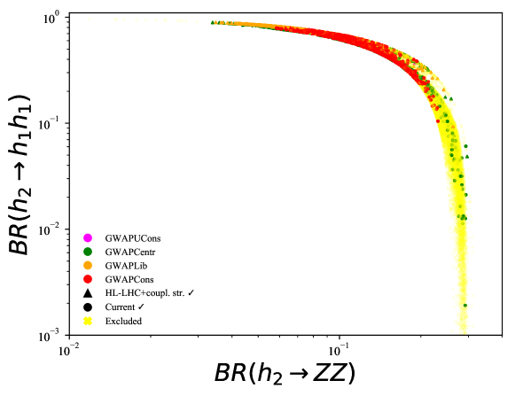
Figure 1: The branching ratio BR$(h_{2}\rightarrow h_{1}h_{1})$ plotted against BR$(h_{2}\rightarrow ZZ)$, over the parameter-space points of the present study for the various categorisations (see section 3.3). We show points that pass the current constraints ($\CIRCLE$) or the HL-LHC constraints plus future signal strength ($|\sin\theta|<0.1$) constraints ($\blacktriangle$), as well as those that are currently excluded (faint $\color[rgb]{1,1,0}\boldsymbol{\times}\color[rgb]{0,0,0}$).

We discuss the decay modes of the $h_{2}$ boson within the context of our study in detail in appendix A. Here, we wish emphasise the complementarity between the decay modes $h_{2}\rightarrow h_{1}h_{1}$ and $h_{2}\rightarrow VV$ ($V=Z,W$), exemplified by fig. 1, where the branching ratio of BR$(h_{2}\rightarrow h_{1}h_{1})$ is plotted against BR$(h_{2}\rightarrow ZZ)$, over the parameter-space points of the present study (see section 3.3 for their definitions). From fig 1, it also becomes clear that since the $h_{2}\rightarrow ZZ$ decay (and hence $h_{2}\rightarrow W^{+}W^{-}$) never becomes less frequent than $\mathcal{O}(\mathrm{few}~{}\%)$, it is has the potential to be overall a more powerful probe of the parameter space than $h_{2}\rightarrow h_{1}h_{1}$, which can attain small BR values, down to $\mathcal{O}(10^{-3})$. We also note that there are exist viable SFO-EWPT parameter-space points with $m_{2}<2m_{1}$, where $h_{1}h_{1}$ production is not kinematically allowed. In appendix A we show an alternative view of the complementarity between the $h_{1}h_{1}$ and $ZZ$ final states, through the ratio of BR$(h_{2}\rightarrow h_{1}h_{1})$/BR$(h_{2}\rightarrow ZZ)$ versus the mass of $h_{2}$, in the bottom-right panel of fig. 8.

3 Calculating the order of the phase transition

Perturbative methods of treating the effective potential at finite temperature suffer from both gauge [70] and a break down of perturbation theory [71]. The breakdown of perturbation theory arises due to Linde’s infamous infrared problem – during the phase transition as the expansion parameter is not the actual coupling but the coupling multiplied by the mode occupation instead: $gn_{B}\sim gT/m$ (where $T$ is the temperature, $n_{B}$ is the mode occupation, $m$ is a mass and $g$ is some coupling), which clearly diverges for $m\to 0$. A probe of how well perturbation theory is working is to measure the scale dependence of the theory. If perturbation theory is converging quickly, we can define our potential at one loop order and the scale dependence from running should approximately cancel the scale dependence at one loop, any remaining scale dependence is formally higher order. A large sensitivity therefore shows that the theory is particularly sensitive to higher-loop corrections which points to the failure of perturbation theory to converge quickly.

The scale dependence is the dominant theoretical uncertainty if one keeps within the perturbative region of the theory [57]. A partial solution to the scale dependence is to perform a resummation of the masses. Doing so makes the uncertainty in the critical temperature of the SM effective theory non-trivial but manageable, in contrast to the uncertainty in the gravitational wave amplitude generated from a first-order transition which is at the multi-order of magnitude level [57]. In the present paper we consider bosons that couple to the SM with potentially large couplings - in fact past papers that studied the EWPT, considered portal couplings of $K_{2}\sim\mathcal{O}(10)$ [52]. For that reason we expect the theoretical uncertainties even in the strength of the phase transition to be very large.

The gauge dependence can be avoided via an expansion in the Planck constant, $\hbar$, instead of the usual loop expansion, but unless one expands to second order in $\hbar$, the scale dependence is unmanageable [72]. Going to two loops is cumbersome and we will not pursue it here as a solution. Another solution is to integrate out the heavy “Matsubara” modes, which results in a theory that is effectively three-dimensional [74, 75, 76, 77, 78, 79, 80, 81, 82, 83, 84, 85, 86]. The dimensionally-reduced theory is manifestly gauge-invariant and includes all-orders of resummation, resulting in a substantial reduction in the uncertainties [57]. For the SM extended by a real singlet scalar field, there can be two light dynamical modes, rendering the analysis a theoretical challenge that we leave to future work.

Here we instead advocate to analyse the electro-weak phase diagram within a given model via an approach that balances convenience, while limiting theoretical uncertainties. Given that we are interested in assessing the order of the phase transition and not gravitational wave phenomenology, the uncertainties are often large but nonetheless manageable in the usual four-dimensional perturbative calculation, where the gauge and scale dependence are treated as theoretical uncertainties.

To assess the question whether a collider rules out a SFO-EWPT, we consider the maximum value of the order parameter, requiring

$${\rm Max}\left(\frac{\Delta h}{T_{C}}\right)>1\;,$$ (3.1)

for a given parameter point with physical quantities matched at the $Z$ pole and with the renormalisation scale and gauge parameters varied. In the above, $T_{C}$ is the critical temperature at which the theory has a degenerate ground state and $\Delta h$ is the difference in the Higgs field between the two vacua at the critical temperature. By contrast, to assess the discovery prospects we instead look at the minimum value, requiring

$${\rm Min}\left(\frac{\Delta h}{T_{C}}\right)>1\;,$$ (3.2)

when varying over the same range of the scale and gauge parameters. It is therefore useful to classify which points might be strongly first order, as they sometimes are when vary scale and gauge parameters, and when they are robust to theoretical uncertainties. The specific implementation of this and how we categorise our points we discuss in section 3.3.

3.1 Gauge and Scale Dependence

To capture the theoretical uncertainties coming from the gauge dependence, we construct the effective potential in the general covariant gauge (also known as Fermi gauges) rather than the usual $R_{\xi}$ gauge [87]. The $R_{\xi}$ gauge uses a different gauge for every value of the scalar field(s). It is not a priori clear that this is possible [88, 89]. To construct the potential we follow the techniques of ref. [87].

The potential at one loop in the covariant gauge is given by

$$V_{\rm 1-loop}=V_{\rm tr}(h,s,Q)+V_{\rm CW}(h,s,Q,\xi_{W},\xi_{B})+V_{T}(h,s,Q,\xi_{W},\xi_{B})\;,$$ (3.3)

where $V_{\rm tr}$ is the tree-level potential, $V_{\rm CW}$ the Coleman-Weinberg (CW) term, $V_{T}$ the thermal term, $Q$ is the renormalisation scale and the $\xi_{i}$ ($i=W,B$) are the gauge parameters. The remaining details of the effective potential at finite temperature in the covariant gauge are given in appendix B.

To minimise scale dependence, we use “Arnold-Espinosa” resummation [73] of the masses and allow all parameters in the effective potential to run. We use the program SARAH [90] to derive the one-loop renormalisation group equations (RGEs) and we vary the RGE scale, $Q$, that defines the coupling and the CW potential, by an order of magnitude: $m_{Z}/2<Q<m_{Z}\times 5$, where $m_{Z}$ is the $Z$ boson mass.

3.2 Numerical calculation of the phase transition

PhaseTracer is a publicly-available C++ package [91] that traces the thermal evolution of the effective potential using the algorithm developed in ref. [92]. It was designed to be robust, with an improved treatment of thermal functions [93] and discrete symmetries.

We have developed a module for PhaseTracer for the real scalar singlet extension of the SM in the covariant gauge with “Arnold-Espinosa” resummation of thermal masses. Since the choice of gauge only enters the effective potential through the field-dependent masses, the covariant gauge can be readily implemented in PhaseTracer by simply providing expressions for these. We can then treat the gauge parameters as inputs we vary.

The requirement that we have a SFO-EWPT typically requires large portal couplings, which implies that the unphysical scale dependence at one loop can become quite large, even at zero temperature. This, in addition to the unphysical gauge dependence of the minimum calculated at one loop, motivates a generous tolerance for the zero-temperature vev value of the Higgs field. In particular, if we wish to claim that a certain collider can exclude the possibility of the cosmological phase transition being strongly first order, we choose to be liberal and not too aggressive in excluding points that could be potential candidates. We discuss our analysis of the phase structure in detail in the next sub-section.

3.3 Parameter-space categorisation

Parameter	Range
$\lambda_{s}$	$[10^{-4},3]$
$K_{1}$	$[-2000,0]$ GeV
$K_{2}$	$[0,10]$
$M_{S}$	$[-2000,2000]$ GeV
$\kappa$	$-[1800,1800]$ GeV

Table 1: The range of parameters used in our scans of the parameter space of the real singlet scalar extension of the SM.

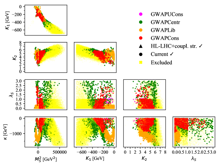
Figure 2: Two-dimensional projections of the parameter space showing points obtained in our scan for the five free parameters that we scanned over. We show points that pass the current constraints ($\CIRCLE$) or the HL-LHC constraints plus future signal strength ($|\sin\theta|<0.1$) constraints ($\blacktriangle$), as well as those that are currently excluded (faint $\color[rgb]{1,1,0}\boldsymbol{\times}\color[rgb]{0,0,0}$).

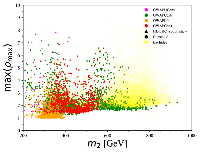
Figure 3: The maximum value of $\rho_{\mathrm{max}}=\phi_{C}/T_{C}$ over the set of eight scale/gauge variations for each of the parameter-space points against the mass of $h_{2}$, $m_{2}$. We show points that pass the current constraints ($\CIRCLE$) or the HL-LHC constraints plus future signal strength ($|\sin\theta|<0.1$) constraints ($\blacktriangle$), as well as those that are currently excluded (faint $\color[rgb]{1,1,0}\boldsymbol{\times}\color[rgb]{0,0,0}$).

To derive parameter-space points that satisfy SFO-EWPT, we perform random scans over the five free parameters in the potential. We generate points with viable zero-temperature phenomenology, leaving a large leeway for theoretical uncertainties. Table 1 presents our scan range, which was performed for $\mathcal{O}(10^{6})$ points. We impose a cutoff on dimensionful parameters, at around 2 TeV, as well as on the dimensionless portal coupling $K_{2}$, in order to lie well below the perturbativity bound. This is because the theoretical uncertainties become unmanageable for larger couplings and large scale hierarchies. Note that our scan does not represent a uniform sampling of the parameter space: this implies that our results should not be interpreted so as to indicate densities of points in parameter space, but rather to map out its boundaries. We create a set of eight points for each parameter point with $\{\mu,\xi_{W,Z}\}\in\{(m_{Z}/2,m_{Z},2m_{Z},5m_{Z}),(0,3)\}$. We require the Higgs boson mass to equal $125.1$ GeV at $\mu=m_{Z},~{}\xi_{W,Z}=0$ and we impose a restriction on the one-loop value of the sine of the mixing angle: $|\sin\theta|<0.25$. Each of the eight points is individually passed to PhaseTracer for further processing. PhaseTracer calculates the phases and the transitions between them. The transitions are classified according to the value of $\rho=\phi_{C}/T_{C}$, where $\phi_{C}$ is the Higgs field vev and $T_{C}$ is the critical temperature.

PhaseTracer has multiple advantages [91] over CosmoTransitions [92]. However, PhaseTracer does not calculate the nucleation rate at present. We therefore consider approximate criteria in categorizing a strong first order phase transition. If there exist phase transitions with $T_{c}>30$ GeV and $\rho>1$, and no other transitions with $\rho\in[0.1,1.0]$ with higher $T_{c}$ than the $\rho>1.0$ transition, then we label a point as satisfying the “SFO condition”. Additionally, the maximum value of $\rho$, denoted as $\rho_{\mathrm{max}}$, is kept for each of the eight scale/gauge variations. Furthermore, if for an individual point there exists a Higgs field vev within $v_{0}=246\pm 30$ GeV, that also corresponds to a transition to the absolute (i.e. deepest) minimum of the potential, we label it as satisfying the “first type of vev condition”. The subset of points that satisfy the “SFO condition” are considered for additional post-processing. We also save the value of the Higgs field vev at the deepest minimum for each of these points. During the post-processing of the points, we also consider an additional property, pertaining to the group of eight scale/gauge variations: if at least one point has for the deepest minimum $v_{0}<246$ GeV and another has for the deepest minimum $v_{0}>246$ GeV, we label it as satisfying the “second type of vev condition”. We use these conditions to categorise the points. To best take into account the theoretical uncertainties, we consider two types of classification. The first type of classification separates points into:

• Ultra-Conservative points: all eight of them satisfy the SFO and all eight also satisfy the first type of vev condition.

• Conservative points: all eight of them have to satisfy SFO and at least one point has to satisfy the first type of vev condition. Ultra-Conservative points are excluded from this category.

• Centrist points: at least one point within the eight satisfying SFO and first type of vev conditions simultaneously. (Ultra-)Conservative points are excluded from this category.

• Liberal points: at least one point within the eight satisfies SFO and any other satisfies the first type of vev conditions. Centrist and (Ultra-)Conservative points are excluded from this category.

The second classification separates points into two mutually-exclusive categories:

• Tight points: all eight of them have to satisfy SFO and the group has to satisfy the second type of vev condition.

• Loose points: at least one point within the eight satisfying SFO and the group has to satisfy the second type of vev condition.

In the main part of the article we show results for the first type of classification (GWAPUCons, GWAPCons, GWAPCentr and GWAPLib as defined above, respectively), with a selection of results for the second type (GWAPTight, GWAPLoose, respectively) shown in Appendix G. Our results show that the “Centrist” and “Loose” categories behave in a similar fashion, whereas the “Liberal” category of the first classification has no correspondence in the second and allows for larger theoretical uncertainties.

We show two-dimensional projections of the parameter-space points obtained in our scan, for the five free parameters that we scanned over in fig. 2. Notice that the theoretical uncertainties get large when there is either a large scale hierarchy (including a large ratio of dimensionful parameters) or a large dimensionless coupling. Specifically if $\lambda_{s}\gtrsim 2$ or $K_{2}\gtrsim 4$ then the theoretical uncertainties begin to get large. This is precisely what is to be expected if the uncertainties mostly arise due to the unphysical scale dependence coming from the breakdown of perturbativity. In fig. 3 we show the resulting maximum value of $\rho_{\mathrm{max}}$ over the eight scale and gauge variations for each of the parameter-space points. In both figs. 2 and 3 we show points that pass the current constraints ($\CIRCLE$) or the HL-LHC constraints plus future signal strength ($|\sin\theta|<0.1$) constraints ($\blacktriangle$), as well as those that are currently excluded (faint $\color[rgb]{1,1,0}\boldsymbol{\times}\color[rgb]{0,0,0}$), see the next section and the relevant appendices for further clarification of these conditions. We emphasise that, in all of the phenomenological studies that follow, we employ the “central” parameter-space point in the group, i.e. with $\{\mu,\xi_{W,Z}\}=\{m_{Z},0\}$, irrespective of whether it satisfies the above conditions.

4 Summary of collider constraints

There exist several categories of collider constraints that affect the parameter space of the real singlet extension of the SM. These come through direct searches for heavy scalar resonances (i.e. $h_{2}$), SM-like Higgs boson signal strength measurements (i.e. $h_{1}$) and electro-weak precision observables. To assess the potential of future colliders for exclusion or discovery of the real singlet model in the context of a SFO-EWPT, at the end of the lifetime of the high-luminosity run of the LHC (HL-LHC), we consider the most up-to-date collider constraints coming from these categories.

To impose current constraints coming from heavy Higgs boson searches and Higgs boson measurements, we employ the HiggsBounds [95, 96, 97, 98] and HiggsSignals [99, 100, 101] packages. In addition, we consider constraints coming from resonant Higgs boson pair production, $h_{2}\rightarrow h_{1}h_{1}$ and also incorporate the latest 13 TeV ATLAS and CMS SM-like Higgs boson global signal strengths, $\mu=\sigma^{\mathrm{measured}}/\sigma^{\mathrm{SM}}$, that are currently not included in HiggsSignals. Further details on these can be found in Appendix C.

For the HL-LHC, we consider the prospects for the Higgs boson signal strength measurement, as well as various analyses assessing the heavy Higgs boson prospects of the HL-LHC in final states originating from $h_{2}\rightarrow h_{1}h_{1}$, $h_{2}\rightarrow ZZ$ and $h_{2}\rightarrow W^{+}W^{-}$. We combine these with extrapolations of results from 13 TeV where appropriate. For further details, see Appendix D.

Electron-positron colliders may also provide relevant constraints on the model. In particular, electro-weak precision observable measurements (EWPO) coming from LEP and future lepton colliders, such as the International Linear Collider (ILC) can also probe the effects of new scalar particles. To consider these, we follow the treatment of refs. [29, 52, 53]. We found the resulting constraints to be generally weaker than either the direct heavy Higgs boson searches or the Higgs signal strength measurements and we defer the detailed description and results to Appendix E. There, we also discuss phenomenological results obtained for the Compact Linear Collider (CLIC) [58], which we briefly contrast to the hadron collider results.

To derive the prospects of future hadron colliders to either discover or rule out the real singlet extension of the SM in regards to SFO-EWPT, we have constructed detailed phenomenological analyses at the Monte Carlo level, considering the processes $h_{2}\rightarrow h_{1}h_{1}$, $h_{2}\rightarrow ZZ$ and $h_{2}\rightarrow W^{+}W^{-}$ at a 100 TeV proton collider in the mass range $m_{2}\in[200,1000]$ GeV. These were inspired by current LHC analyses, with appropriate modifications at 100 TeV. To obtain the HE-LHC constraints we have performed an extrapolation of the 100 TeV results down to 27 TeV. These phenomenological analyses and associated results are discussed in detail in Appendix F.

To estimate the future colliders constraints on the mixing angle through signal strength measurements, we note the several signal strength and coupling measurement projections for various channels that are found in ref. [102]. These point towards a $\mathcal{O}(1\%)$ uncertainty or better at electron-positron colliders and at a 100 TeV proton collider. In the absence of a full signal strength combination at these colliders, to remain conservative, we will assume the 95% C.L. constraint $\sin^{2}\theta<0.01$. We apply this constraint in addition to those coming from direct searches for heavy Higgs bosons at future colliders.

Throughout this article we will only show parameter-space points that pass the current constraints described in detail in Appendix C (denoted by a $\CIRCLE$), or the HL-LHC constraints described in detail in Appendix D plus future signal strength ($|\sin\theta|<0.1$) constraints (denoted by a $\blacktriangle$). For completeness, we also show those that are currently excluded (faint $\color[rgb]{1,1,0}\boldsymbol{\times}\color[rgb]{0,0,0}$) without indicating the category they fall into.

5 Phenomenological results

5.1 Theoretical uncertainties

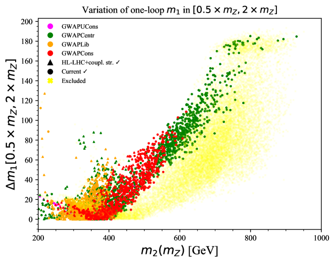
Figure 4: The change of the one-loop SM-like Higgs boson ($h_{1}$) mass, $m_{1}$, with scale taken in $[0.5m_{Z},2m_{Z}]$. We show points that pass the current constraints ($\CIRCLE$) or the HL-LHC constraints plus future signal strength ($|\sin\theta|<0.1$) constraints ($\blacktriangle$), as well as those that are currently excluded (faint $\color[rgb]{1,1,0}\boldsymbol{\times}\color[rgb]{0,0,0}$).

To assess the severity of the theoretical uncertainties at the (zero-temperature) phenomenological level, we have calculated the variation of the one-loop mass of the SM-like Higgs boson with scale, $\Delta m_{1}$, taken in $[0.5m_{Z},2m_{Z}]$. The resulting values are shown in fig. 4. One can observe that the “Conservative” points generally possess a lower variation, $\Delta m_{1}\lesssim 80$ GeV, whereas the “Centrist” plus the “Liberal” points possess variations as large as 100 GeV at $\sim 600$ GeV, which then reach 150–200 GeV around $m_{2}\sim 900$ GeV. It is also evident that the current constraints “push” the parameter-space points towards higher theoretical uncertainties, removing a large proportion of the higher-$m_{2}$ points with a relatively lower value of the variation.

5.2 Future collider prospects

5.2.1 Proton colliders at 100 TeV

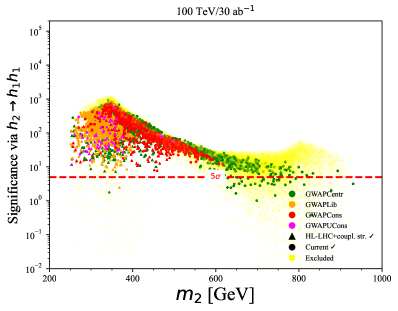
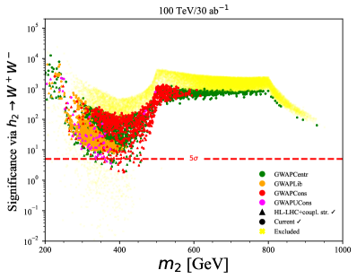
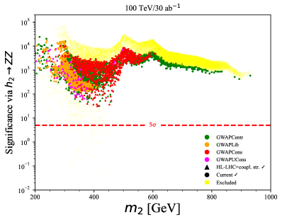
Figure 5: The statistical significances for a heavy Higgs boson ($h_{2}$) signal at a 100 TeV collider with an integrated luminosity corresponding to $30$ ab^-1, for each of individual analyses: $pp\rightarrow h_{2}\rightarrow h_{1}h_{1}$, $pp\rightarrow h_{2}\rightarrow W^{+}W^{-}$ and $pp\rightarrow h_{2}\rightarrow ZZ$. We indicate the $5\sigma$ (discovery) boundaries by the red dashed lines. We show points that pass the current constraints ($\CIRCLE$) or the HL-LHC constraints plus future signal strength ($|\sin\theta|<0.1$) constraints ($\blacktriangle$), as well as those that are currently excluded (faint $\color[rgb]{1,1,0}\boldsymbol{\times}\color[rgb]{0,0,0}$).

Following the Monte Carlo-level phenomenological analyses for $h_{2}$ resonant searches we have developed, presented in Appendix F in detail, we have derived the expected statistical significance at a 100 TeV proton-proton collider, for each of the parameter-space points for a lifetime integrated luminosity of 30 ab^-1. The significances for each of the individual analyses: $pp\rightarrow h_{2}\rightarrow h_{1}h_{1}$, $pp\rightarrow h_{2}\rightarrow W^{+}W^{-}$ and $pp\rightarrow h_{2}\rightarrow ZZ$ are shown in fig. 5. It is evident that the $pp\rightarrow h_{2}\rightarrow h_{1}h_{1}$ process can probe a large part of the parameter space, at an integrated luminosity of 30 ab^-1 on its own, apart from a limited number of points, mostly at higher values of $m_{2}$. The $pp\rightarrow h_{2}\rightarrow ZZ$ and $pp\rightarrow h_{2}\rightarrow W^{+}W^{-}$ channels yield high significances even for points with a large branching ratio $h_{2}\rightarrow h_{1}h_{1}$. This is due to the fact that the parameter-space branching ratios for $h_{2}\rightarrow ZZ$ and $h_{2}\rightarrow W^{+}W^{-}$ remain relatively significant, at least $\mathcal{O}(\mathrm{few}~{}\%)$, even for large BR$(h_{2}\rightarrow h_{1}h_{1})$, and due to the power of the gauge boson analyses themselves. In turn, the $pp\rightarrow h_{2}\rightarrow ZZ$ analysis performs better than the $pp\rightarrow h_{2}\rightarrow W^{+}W^{-}$ analysis that we have constructed, which fails to yield high enough significances for discovery in the intermediate mass range. The sensitivity of the $ZZ$ analyses is driven by the $ZZ\rightarrow(2\ell)(2\nu)$ channel, which yields the most stringent constraints on the $pp\rightarrow h_{2}\rightarrow ZZ$ cross section. The $ZZ$ analysis itself represents by far the highest significance for any parameter-space point.

5.2.2 Proton colliders at 27 TeV

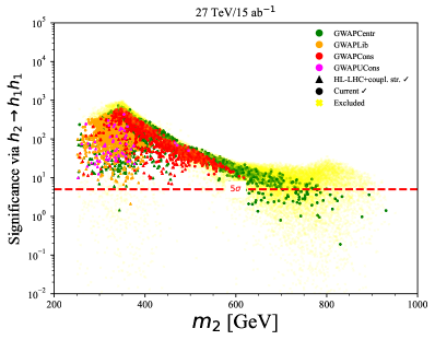
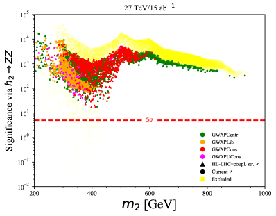
Figure 6: The statistical significances for a heavy Higgs boson ($h_{2}$) signal at 27 TeV collider with an integrated luminosity corresponding to $15$ ab^-1, for each of individual analyses: $pp\rightarrow h_{2}\rightarrow h_{1}h_{1}$, $pp\rightarrow h_{2}\rightarrow W^{+}W^{-}$ and $pp\rightarrow h_{2}\rightarrow ZZ$. We indicate the $5\sigma$ (discovery) boundaries by the red dashed lines. We show points that pass the current constraints ($\CIRCLE$) or the HL-LHC constraints plus future signal strength ($|\sin\theta|<0.1$) constraints ($\blacktriangle$), as well as those that are currently excluded (faint $\color[rgb]{1,1,0}\boldsymbol{\times}\color[rgb]{0,0,0}$).

Following the extrapolation described in appendix F.2, we show equivalent plots for the significances obtained in the $h_{1}h_{1}$ and gauge boson channels in fig. 6, for the case of the HE-LHC 27 TeV proton-proton collider with an integrated luminosity of 15 ab^-1. It is evident that a 27 TeV collider could be powerful enough to exclude or discover a large fraction of the SFO-EWPT parameter space, with reductions in significance of $\mathcal{O}(\mathrm{a~{}few})$. We emphasise, however, that this result should be validated by a full phenomenological analysis, taking into account the signal and background kinematics at 27 TeV.

5.2.3 Summary

It is evident that both a 27 TeV collider with an integrated luminosity of 15 ab^-1 and a 100 TeV collider with 30 ab^-1 may be able to exclude or discover the whole of the parameter-space points. We note that since the 27 TeV result originates in an extrapolation down from 100 TeV/30 ab^-1, it is essential that future studies verify this directly through detailed phenomenological analyses that take into account the changes in kinematics at 27 TeV directly. Nevertheless, it is clear that a 100 TeV machine possesses the power to potentially quite efficiently discover the real singlet scalar extension of the SM. The very high statistical significances found all over the parameter space, particularly in the $ZZ$ final state, point to an early discovery. This would allow for further precise measurements of the properties of the heavy scalar to be obtained during the lifetime of a 100 TeV machine, so as to definitively verify whether indeed this is the physical remnant of a real singlet scalar field that catalyses SFO-EWPT.

5.3 Selected benchmark points

(Ultra-)Conservative benchmarks
Name	UCons1	UCons2	Cons1	Cons2	Cons3	Cons4
$\mathbold{x_{0}}$ [GeV]	49.2	48.8	36.3	46.2	40.1	35.0
$\mathbold{\mu^{2}}$ [GeV2]	-2204.7	-1466.7	-3328.2	-2146.1	-3407.8	-7955.2
$\mathbold{M_{S}^{2}}$ [GeV2]	-8129.0	77814.0	53473.6	98974.7	100232.2	160581.1
$\mathbold{K_{1}}$ [GeV]	-204.3	-299.5	-228.1	-357.1	-336.7	-358.9
$\mathbold{K_{2}}$	4.33	4.53	5.35	4.61	5.58	5.75
$\mathbold{\kappa}$ [GeV]	-61.0	-219.0	-229.1	-23.47	-17.6	-37.1
$\mathbold{\lambda_{S}}$	0.52	-0.0002	0.25	0.45	0.08	0.26
$\mathbold{\lambda}$	0.15	0.16	0.03	0.17	0.02	0.01
max$\mathbold{(\rho_{\mathrm{max}})}$	1.58	2.05	1.49	2.24	1.88	3.43
sin$\mathbold{\theta}$	-0.034	0.138	0.068	0.152	0.118	0.129
$\mathbold{m_{2}}$ [GeV]	377.5	466.29	480.3	527.0	550.8	617.5
$\mathbold{\Gamma_{2}}$ [GeV]	0.098	1.686	0.604	2.32	1.89	2.69
BR($\mathbold{ZZ}$)	0.074	0.147	0.109	0.197	0.167	0.207
BR($\mathbold{W^{+}W^{-}}$)	0.161	0.309	0.228	0.410	0.347	0.427
BR($\mathbold{h_{1}h_{1}}$)	0.736	0.430	0.578	0.246	0.364	0.234
BR($\mathbold{t\bar{t}}$)	0.028	0.11	0.085	0.148	0.121	0.131
$\mathbold{\sigma_{13}}$ [pb]	0.012	0.113	0.024	0.085	0.041	0.030
$\mathbold{\sigma_{27}}$ [pb]	0.060	0.535	0.115	0.399	0.195	0.143
$\mathbold{\sigma_{100}}$ [pb]	0.497	4.873	1.062	3.880	1.948	1.532

Table 2: The “(Ultra-)Conservative” benchmark points (UCons1–Ucons2) Cons1–Cons4 in increasing mass of the $h_{2}$ from left to right. The top panel shows the real singlet-extended SM potential parameters and the bottom panel shows some useful derived quantities, including the significant branching ratios and the gluon-fusion cross sections at 13, 27 and 100 TeV. Note that conservative points have tend to have reasonably large $K_{2}$ and no large hierarchies of scale either in $M_{S}/|\mu|$ or $K_{1}/|\mu|$.

Centrist benchmarks
Name	Centr1	Centr2	Centr3	Centr4	Centr5	Centr6
$\mathbold{x_{0}}$ [GeV]	3.84	26.65	17.9	43.1	38.9	39.7
$\mathbold{\mu^{2}}$ [GeV2]	-6665.1	-4711.8	-5997.3	-1724.8	-3701.0	-13203.1
$\mathbold{M_{S}^{2}}$ [GeV2]	-46929.5	-7926.1	9804.3	96682.3	117494.1	291088.2
$\mathbold{K_{1}}$ [GeV]	0.06	-76.3	-89.1	-289.4	-374.1	-432.9
$\mathbold{K_{2}}$	4.06	5.22	4.85	5.60	5.55	6.07
$\mathbold{\kappa}$ [GeV]	-603.2	-1488.3	-205.7	-787.6	-122.7	-650.5
$\mathbold{\lambda_{S}}$	0.004	-0.0003	1.75	1.485	1.487	0.897
$\mathbold{\lambda}$	0.196	0.125	0.088	0.022	0.029	0.022
max$\mathbold{(\rho_{\mathrm{max}})}$	2.73	1.52	1.33	3.03	3.40	1.73
sin$\mathbold{\theta}$	-0.050	-0.055	0.006	0.098	0.115	0.146
$\mathbold{m_{2}}$ [GeV]	299.6	364.7	434.8	528.1	605.8	732.9
$\mathbold{\Gamma_{2}}$ [GeV]	0.133	0.185	0.004	1.479	1.925	5.002
BR($\mathbold{ZZ}$)	0.046	0.087	0.202	0.130	0.215	0.247
BR($\mathbold{WW}$)	0.104	0.188	0.404	0.271	0.444	0.506
BR($\mathbold{h_{1}h_{1}}$)	0.849	0.704	0.349	0.501	0.201	0.127
BR($\mathbold{t\bar{t}}$)	0.0	0.020	0.043	0.098	0.140	0.120
$\mathbold{\sigma_{13}}$ [pb]	0.024	0.032	0.0003	0.0355	0.0255	0.1572
$\mathbold{\sigma_{27}}$ [pb]	0.114	0.159	0.001	0.166	0.123	0.080
$\mathbold{\sigma_{100}}$ [pb]	0.893	1.291	0.012	1.616	1.299	0.956

Table 3: The “Centrist” benchmark points Centr1–Centr6 in increasing mass of the $h_{2}$ from left to right. The top panel shows the real singlet-extended SM potential parameters and the bottom panel shows some useful derived quantities, including the significant branching ratios and the gluon-fusion cross sections at 13, 27 and 100 TeV. The extra theoretical uncertainty is mostly driven by the large hierarchies in scale - either a large $|M_{S}|/|\mu|$ or a large $K_{1}/|\mu|$.

We present a selection of benchmark points within the “(Ultra-)Conservative” and “Centrist” categories that we have defined in section 3.3. These represent the (very) “low” and “medium” theoretical uncertainty categories of points. Tables 2 and 3 show these points in increasing mass of the $h_{2}$ from left to right. The top panel shows the real singlet-extended potential parameters and the bottom panel shows some useful derived quantities: the maximum value of $\rho_{\mathrm{max}}$ over the variations of scale and gauge parameters, $\sin\theta$, the width of $h_{2}$, the significant branching ratios of $h_{2}$ and the gluon-fusion production cross sections of $h_{2}$ at 13, 27 and 100 TeV. The cross sections are given at NNLO+NNLL according to the CERN “Yellow Report 4” [104] at 13 TeV and calculated at N³LO+NNLL as described in Appendix F.1 via the ihixs program (v2.0) [105] at 27 TeV and 100 TeV. We also show the branching ratio to top quarks, which was not part of our analysis. It is nevertheless of interest, as it could provide the only direct way to measure the coupling of the $h_{2}$ to fermions.

6 Conclusions

We have performed a multi-channel analysis of the electro-weak phase transition at future colliders utilising the real scalar extension of the SM as the test model. Considering decays into vector bosons dramatically improves the reach of colliders to the point that a substantially “weaker” collider, particularly in terms of the integrated luminosity, may be needed to probe the nature of the electro-weak transition than previously thought. This is true even when theoretical uncertainties are taken into account, dramatically expanding the potentially relevant parameter space.

However, it is not clear that the entire relevant parameter space can be probed, as theoretical uncertainties become unmanageable for large scale hierarchies and/or large portal couplings. Improved techniques, such as a higher-loop expansion, an improved resummation or dimensional reduction, will be needed to verify if the real singlet extension of the SM can indeed catalyse the eletro-weak transition within its viable parameter space. Furthermore, an improved analysis could probe larger portal couplings than we were able to consider here. Nevertheless, we emphasise that the present treatment of theoretical uncertainties is generous, and we expect our conclusions to be robust.

Finally, if a new heavy scalar particle is discovered early on at any future collider experiment, as our studies indicate, the challenge would then be to comprehend whether it is indeed the remnant of a new scalar field related to the electro-weak phase transition. This endeavour, part of the so-called “inverse” problem, should be pursued in future investigations.

Appendix A Heavy Higgs boson decay modes

Since we concentrate on the scenario $m_{2}>m_{1}$, no new decay modes appear for the $h_{1}$. For $m_{2}\geq 2m_{1}$, the $h_{2}\rightarrow h_{1}h_{1}$ decay mode opens up, with width:

$$\Gamma_{h_{2}\rightarrow h_{1}h_{1}}=\frac{\lambda^{2}_{112}\sqrt{1-4m_{1}^{2}/m_{2}^{2}}}{8\pi m_{2}}\;,$$ (A.1)

where $\lambda_{112}$ is the $h_{1}-h_{1}-h_{2}$ coupling contained in the scalar potential after electroweak symmetry breaking, $V(h_{1},h_{2})\supset\lambda_{112}h_{1}h_{1}h_{2}$, and $m_{1}$, $m_{2}$ are the masses of the $h_{1}$ and $h_{2}$ particles, respectively. For completeness, we give the full list of the tree-level triple couplings between the scalars $h_{1}$ and $h_{2}$, representing terms of the form $V(h_{1},h_{2})\supset\lambda_{ijk}h_{i}h_{j}h_{k}$, $i,j,k=\{1,2\}$ (see, e.g. [106]):

$$\lambda_{111} = \lambda v_{0}c_{\theta}^{3}+\frac{1}{2}(K_{1}+K_{2}x_{0})c_{\theta}^{2}s_{\theta}\;,$$

$$+ \frac{1}{2}K_{2}v_{0}s_{\theta}^{2}c_{\theta}+\left(\frac{\kappa}{3}+2\lambda_{S}x_{0}\right)s_{\theta}^{3}\;,$$

$$\lambda_{112} = v_{0}(K_{2}-6\lambda)c_{\theta}^{2}s_{\theta}-\frac{1}{2}K_{2}v_{0}s_{\theta}^{3}$$

$$+ (-K_{1}-K_{2}x_{0}+\kappa+6\lambda_{S}x_{0})c_{\theta}s_{\theta}^{2}+\frac{1}{2}(K_{1}+K_{2}x_{0})c_{\theta}^{3}\;,$$

$$\lambda_{122} = v_{0}(6\lambda-K_{2})s_{\theta}^{2}c_{\theta}+\frac{1}{2}K_{2}v_{0}c_{\theta}^{3}$$

$$+ (\kappa+6\lambda_{S}x_{0}-K_{1}-K_{2}x_{0})s_{\theta}c_{\theta}^{2}+\frac{1}{2}(K_{1}+K_{2}x_{0})s_{\theta}^{3}\;,$$

$$\lambda_{222} = \frac{1}{12}\left[4(\kappa+6\lambda_{S}x_{0})c_{\theta}^{3}-6K_{2}v_{0}c_{\theta}^{2}s_{\theta}\right.$$

$$+ \left.6(K_{1}+K_{2}x_{0})c_{\theta}s_{\theta}^{2}-24\lambda v_{0}s_{\theta}^{3}\right]\;,$$

where we have defined $c_{\theta}\equiv\cos\theta$ and $s_{\theta}\equiv\sin\theta$.

The total width of the $h_{2}$ scalar is given by:

$$\Gamma_{h_{2}}=\sin^{2}\theta~{}\Gamma^{\mathrm{SM}}(m_{2})+\Gamma_{h_{2}\rightarrow h_{1}h_{1}}\;,$$ (A.3)

where $\Gamma^{\mathrm{SM}}(m_{2})$ corresponds to the width of a scalar boson of mass $m_{2}$ possessing the same decay modes as the SM Higgs. In what follows, we have used the $\Gamma^{\mathrm{SM}}(m_{2})$ corresponding to the CERN “Yellow Report 4” (YR4) [104], interpolated for intermediate values up to $m_{2}=1000$ GeV. The branching ratios corresponding to $h_{2}\rightarrow xx$, for $x\neq h_{1}$, are then given by:

$$\mathrm{BR}(h_{2}\rightarrow xx)=\sin^{2}\theta\frac{\Gamma_{xx}^{\mathrm{SM}}(m_{2})}{\Gamma_{h_{2}}}\;,$$ (A.4)

where $\Gamma_{xx}^{\mathrm{SM}}(m_{2})$ corresponds to the SM-like width of a scalar boson of mass $m_{2}$ into the final state $xx$, i.e. in the limit $\lambda_{112}\rightarrow 0$. The values $\Gamma_{xx}^{\mathrm{SM}}(m_{2})$ were likewise obtained from the CERN YR4 and interpolated. We note that owing to the current constraints on $\sin\theta$, the width of $h_{2}$ for viable parameter-space points is small compared to its mass. Therefore, throughout this paper, we have assumed that $\Gamma_{h_{2}}\ll m_{2}$.

Figure 7: The value of $\sin\theta$ for each of the parameter-space points against the mass of $h_{2}$, $m_{2}$. We show points that pass the current constraints ($\CIRCLE$) or the HL-LHC constraints plus future signal strength ($|\sin\theta|<0.1$) constraints ($\blacktriangle$), as well as those that are currently excluded (faint $\color[rgb]{1,1,0}\boldsymbol{\times}\color[rgb]{0,0,0}$).

In fig. 7 we show the one-loop value of $\sin\theta$, the most crucial ingredient when calculating the collider production cross sections of $h_{2}$. We note that this can also attain negative values, which dominate the lower-$m_{2}$ region of parameter space. Although the sign of $\sin\theta$ does not affect single scalar production, it has an impact on multi-scalar production processes. The portion of parameter space above $|\sin\theta|\sim 0.16$ is excluded by current experimental results.

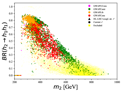
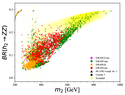
Figure 8: The branching ratios for the heavy Higgs boson, $h_{2}\rightarrow h_{1}h_{1}$ (top right), $h_{2}\rightarrow ZZ$ (top left) and $h_{2}\rightarrow W^{+}W^{-}$ (bottom left) for the parameter-space points in the “Conservative” (red), “Liberal” (orange) and “Centrist” (green) categories, plotted against its mass, $m_{2}$. The bottom right plot shows the ratio of the $h_{2}\rightarrow h_{1}h_{1}$ branching ratio to that of $h_{2}\rightarrow ZZ$. We show points that pass the current constraints ($\CIRCLE$) or the HL-LHC constraints plus future signal strength ($|\sin\theta|<0.1$) constraints ($\blacktriangle$), as well as those that are currently excluded (faint $\color[rgb]{1,1,0}\boldsymbol{\times}\color[rgb]{0,0,0}$).

In fig. 8, we show the branching ratios of the $h_{2}$ for the parameter-space points that we have generated. The “(Ultra-)Conservative” points exhibit a relatively high branching ratio to $h_{2}\rightarrow h_{1}h_{1}$, between $\sim 0.2-0.75$, whereas the “Centrist” plus “Liberal” points span values from $\mathcal{O}(10^{-2})$ up to $\sim 0.9$. The lower-right plot of fig. 8 shows the ratio of the rate to $h_{2}\rightarrow h_{1}h_{1}$ over that to $h_{2}\rightarrow ZZ$. It is clear that the gauge boson final states can play a crucial in discovering or excluding the existence of $h_{2}$, particularly in the higher-mass regions ($m_{2}>600$ GeV), where the decay to $h_{1}h_{1}$ is sub-dominant.

Appendix B One-loop corrections to the effective potential in the covariant gauge

In this appendix we give details about how to derive the effective potential at zero and finite temperature in the covariant gauge (also known as Fermi gauges). We follow the prescription given in ref. [87]. We begin by writing the Higgs doublet components as

$$H=\left(\begin{array}[]{c}\phi_{1}+i\psi_{1}\\ \phi_{2}+i\psi_{2}\end{array}\right)\ .$$ (B.1)

It then becomes useful to write a vector of the five real scalars, including the singlet component which we denote as $s$,

$$\Psi_{a}=\left(\begin{array}[]{c}\phi_{1}\\ \phi_{2}\\ \psi_{1}\\ \psi_{2}\\ s\end{array}\right)\ .$$ (B.2)

Similarly, we write a vector of gauge bosons

$$V_{\mu}=\left(\begin{array}[]{c}W^{1}_{\mu}\\ W^{2}_{\mu}\\ W^{3}_{\mu}\\ B_{\mu}\end{array}\right)\ .$$ (B.3)

The one-loop Lagrangian can be written as:

$${\cal L}_{\rm 1-loop}=V(H,s)-\frac{1}{2}\Phi^{\dagger}\left[\begin{array}[]{cc}D^{ab}&M^{a}_{\mu}\\ M_{\mu}^{a}{}^{\dagger}&\bar{\Delta}_{\mu\nu}\end{array}\right]\Phi+{\cal L}_{\rm fermion}\supset\frac{1}{2}\Phi^{\dagger}\Sigma\Phi\;,$$ (B.4)

where $\Phi=(\Psi_{a},V_{\mu})^{\rm T}$ and

$$D^{ab} = \left(\begin{array}[]{ccccc}-p^{2}+d_{11}&0&0&0&0\\ 0&-p^{2}+d_{22}&0&0&d_{25}\\ 0&0&0-p^{2}+d_{33}&0&0\\ 0&0&0&-p^{2}+d_{44}&0\\ 0&d_{52}&0&0&-p^{2}+d_{55}\end{array}\right)\;,$$ (B.10)

$$M^{a}_{\mu} = \left(\begin{array}[]{cccc}0&\frac{i}{2}g_{2}\phi_{2}p_{\mu}&0&0\\ 0&0&0&0\\ \frac{i}{2}g_{2}\phi_{2}p_{\mu}&0&0&0\\ 0&0&-\frac{i}{2}g_{2}\phi_{2}p_{\mu}&\frac{i}{2}g_{1}\phi_{2}p_{\mu}\\ 0&0&0&0\end{array}\right)\;,$$ (B.16)

$$\bar{\Delta}_{\mu\nu} = \left(\begin{array}[]{cccc}\Delta^{11}_{\mu\nu}&0&0&0\\ 0&\Delta^{11}_{\mu\nu}&0&0\\ 0&0&\Delta^{33}_{\mu\nu}&\Delta^{34}_{\mu\nu}\\ 0&0&\Delta^{43}_{\mu\nu}&\Delta^{44}_{\mu\nu}\end{array}\right)\;,$$ (B.22)

$$d_{11} = d_{22}=d_{33}=d_{44}-\mu^{2}+\frac{\lambda}{2}\phi_{2}^{2}+K_{1}s+\frac{K_{2}}{2}x^{2}\;,$$ (B.23)

$$d_{25} = d_{52}=K_{1}\phi_{2}+\phi_{2}sK_{2}\;,$$ (B.24)

$$d_{55} = \frac{K_{2}}{2}\phi_{2}^{2}+M_{S}^{2}+2s\kappa+6\lambda_{s}s^{2}\;,$$ (B.25)

$$\Delta^{11}_{\mu\nu} = \Delta^{22}_{\mu\nu}=\Delta^{33}_{\mu\nu}g_{\mu\nu}\left(p^{2}-\frac{1}{4}g_{2}^{2}\phi_{2}^{2}\right)-\left(1-\frac{1}{\xi_{W}}p_{\mu}p_{\nu}\right)\;,$$ (B.26)

$$\Delta^{34}_{\mu\nu} = \Delta^{43}_{\mu\nu}=\frac{1}{4}g_{1}g_{2}\phi_{2}^{2}g_{\mu\nu}\;,$$ (B.27)

$$\Delta^{44}_{\mu\nu} = g_{\mu\nu}\left(p^{2}-\frac{1}{4}g_{1}^{2}\phi_{2}^{2}\right)-\left(1-\frac{1}{\xi_{B}}\right)p_{\mu}p_{\nu}\;.$$ (B.28)

Taking the determinant of the matrix $\Sigma$, it is straightforward to derive the mass eigenvalues that enter the one-loop corrections to the tree-level potential:

$$V_{\rm tr}(h,s,Q) = \frac{\mu^{2}(Q)}{2}h^{2}+\frac{\lambda_{h}(Q)}{8}h^{4}$$ (B.29)

$$+\frac{K_{1}(Q)}{2}h^{2}s+\frac{K_{2}(Q)}{4}h^{2}s^{2}$$

$$+\frac{M_{S}(Q)^{2}}{2}s^{2}+\frac{\kappa(Q)}{3}s^{3}+\frac{\lambda_{s}(Q)}{2}s^{4}\;,$$

$$V_{\rm CW}(h,s,Q,\xi_{W},\xi_{B}) = \sum_{i\in\rm scalars}n_{i}\frac{m_{i}^{4}(h,s,Q,\xi_{W},\xi_{B})}{64\pi^{2}}\left[\log\left(\frac{m_{i}^{2}(h,s,Q,\xi_{W},\xi_{B})}{Q^{2}}\right)-\frac{3}{2}\right]$$ (B.30)

$$-\frac{3m_{t}^{4}(h,Q)}{16\pi^{2}}\left(\frac{m_{t}^{2}(h,Q)}{Q^{2}}\right)$$

$$+\sum_{i\in\rm gauge}n_{i}\frac{m_{i}^{4}(h,s,Q)}{64\pi^{2}}\left[\log\left(\frac{m_{i}^{2}(h,s,Q)}{Q^{2}}\right)-\frac{5}{6}\right]\;,$$

$$V_{T}(h,s,Q,\xi_{W},\xi_{B}) = \frac{T^{4}}{2\pi^{2}}\sum_{i}n_{i}J_{B}\left(\frac{m_{i}(h,s,Q,\xi_{W},\xi_{B})}{T^{2}}\right)$$ (B.31)

$$+12\frac{T^{4}}{2\pi^{2}}J_{F}\left(\frac{m_{t}(Q,h)}{T^{2}}\right)\;.$$

In the above, the field-dependent top and gauge boson masses take their usual form. The four Goldstone-like scalar masses and two physical modes are, respectively,

$$m_{1,\pm}^{2} = \frac{1}{2}\left(\chi\pm\sqrt{\chi^{2}-\Upsilon_{W}}\right)\;,$$ (B.32)

$$m_{2,\pm}^{2} = \frac{1}{2}\left(\chi\pm\sqrt{\chi^{2}-\Upsilon_{Z}}\right)\;,$$ (B.33)

$$m_{h,\pm} = \frac{1}{2}\left(-b\pm\sqrt{b^{2}-4c}\right)\;,$$ (B.34)

where

$$\chi = \mu^{2}(Q)+\frac{\lambda(Q)}{2}h^{2}+\frac{K_{2}(Q)}{2}s^{2}+K_{1}(Q)s\;,$$ (B.35)

$$\Upsilon_{W} = \frac{1}{2}\left(2\mu^{2}(Q)+s(2K_{1}(Q)+sK_{2}(Q))+\lambda(Q)h^{2}\right)g_{2}^{2}(Q)h^{2}\xi_{W}\;,$$ (B.36)

$$\Upsilon_{Z} = \frac{1}{2}\left(2\mu^{2}(Q)+s(2K_{1}(Q)+sK_{2}(Q))+\lambda(Q)h^{2}\right)(g_{2}^{2}(Q)\xi_{W}+g_{1}^{2}(Q)\xi_{B})h^{2}\;,$$ (B.37)

$$b = -M_{S}^{2}(Q)-\frac{s}{2}\left(2K_{1}(Q)+sK_{2}(Q)+12\lambda_{s}(Q)s+4\kappa(Q)\right)-\mu^{2}(Q)$$ (B.38)

$$-\frac{h^{2}}{2}\left(K_{2}(Q)+3\lambda(Q)\right)\;,$$

$$c = \frac{1}{4}(2(M_{S}^{2}(Q)+2s(3\lambda_{s}(Q)s+\kappa(Q)))(2K_{1}(Q)sK_{2}(Q)s^{2}2\mu^{2}(Q))$$

$$+(-4K_{1}^{2}(Q)-6K_{1}(Q)K_{2}(Q)s-3K_{2}^{2}(Q)s^{2}$$

$$+6(M_{S}^{2}(Q)+2s(3\lambda_{s}(Q)s+\kappa(Q)))\lambda(Q)+2K_{2}(Q)\mu^{2}(Q))h^{2}+3K_{2}(Q)\lambda(Q)h^{4})\;.$$

Finally, the multiplicities for the scalar masses are $n_{1,+}=n_{1,-}=2$ and $n_{2,\pm}=n_{h,\pm}=1$. The “Arnold-Espinosa” method involves resumming the bosonic masses which results in the addition of Daisy terms to the effective potential

$$V_{D}=-\frac{T}{12\pi}\sum_{i}n_{i}\left(\tilde{m_{i}}^{3}-m_{i}^{3}\right)\;,$$ (B.40)

where we have suppressed gauge, field and scale dependence in the arguments. The scalar Debye masses are given by

$$\Pi_{h} = \left(\frac{\lambda}{4}+\frac{g_{1}^{2}+3g_{2}^{2}}{16}+\frac{y_{t}^{2}}{4}\right)T^{2}\;,$$

$$\Pi_{s} = \frac{\lambda_{s}}{2}T^{2}\;.$$ (B.41)

The scalar masses that go into the Daisy resummation term of the potential are simply $\tilde{m}^{2}=m_{i,\pm}^{2}+\Pi_{h}$ for the four Goldstone-like mass terms. For the physical states, the tilded masses are the eigenvalues of the matrix

$$\left(\begin{array}[]{cc}\frac{\partial^{2}V_{\rm tr}}{dh^{2}}+\Pi_{h}&\frac{\partial^{2}V_{\rm tr}}{dhds}\\ \frac{\partial^{2}V_{\rm tr}}{dhds}&\frac{\partial^{2}V_{\rm tr}}{ds^{2}}+\Pi_{s}\end{array}\right)\ .$$ (B.42)

To remarkable accuracy, one can write the two gauge boson Debye masses as

$$\Pi_{W} = \frac{11}{6}g_{2}^{2}T^{2}\;,$$ (B.43)

$$\Pi_{Z} = \frac{11}{6}\frac{g_{1}^{4}+g_{2}^{4}}{g_{1}^{2}+g_{2}^{2}}\;.$$ (B.44)

Appendix C Current constraints

C.1 Current constraints through HiggsBounds and HiggsSignals

To incorporate an array of current collider constraints into our analysis, we employ the HiggsBounds (v5.9.0) [95, 96, 97, 98] and HiggsSignals (v2.5.1) [99, 100, 101] packages. HiggsBounds takes a selection of Higgs sector predictions for any model as input and then uses the experimental topological cross section limits from Higgs boson searches at LEP, the Tevatron and the LHC to determine if this parameter point has been excluded at 95% C.L.. HiggsSignals performs a statistical test of the Higgs sector predictions of arbitrary models with the measurements of Higgs boson signal rates and masses from the Tevatron and the LHC. HiggsBounds returns a boolean corresponding to whether the Higgs sector passes the constraints at 95% C.L. (true) or not (false). HiggsSignals returns a probability value ($p$-value) corresponding to the goodness-of-fit of the Higgs sector over several SM-like “peak” observables. At present these involve the LHC 13 TeV results of refs. [107, 108, 109, 110, 111, 112, 113, 114, 115, 116].

Effectively, HiggsBounds and HiggsSignals impose constraints through direct SM-like Higgs boson signals ($h_{1}$) and direct searches for heavy scalars ($h_{2}$). The SM-like Higgs boson signals impose constraints through the reduction of the rate via $\cos\theta$ and the $h_{2}$ searches impose constraints on $\sin\theta$ and the branching ratio to a particular final state, according to eq. 2.3. In HiggsBounds, the most constraining analyses have been found to be the CMS combination of SM-like Higgs boson searches and measurements of its properties using 7 and 8 TeV proton-proton centre-of-mass data corresponding to an integrated luminosity of 5.1 fb^-1 and 12.2 fb^-1 respectively [117] ($pp\rightarrow h_{1}$), the ATLAS combination of searches for heavy resonances decaying into bosonic and leptonic final states using 36 fb^-1 of data at 13 TeV [118] ($pp\rightarrow h_{2}\rightarrow VV$), and CMS searches for new scalar resonances decaying to $Z$ boson pairs at 13 TeV with 35 fb^-1 of data [119] ($pp\rightarrow h_{2}\rightarrow ZZ$).

C.2 Current constraints through resonant $h_{2}\rightarrow h_{1}h_{1}$

To supplement the HiggsBounds and HiggsSignal constraints we consider in addition the searches of resonant SM-like Higgs boson pair production conducted by ATLAS [120] and CMS [121]. These searches consider combinations of searches for resonant Higgs boson pair production at 13 TeV centre-of-mass energy, using 36.1 fb^-1 and 35.9 fb^-1 of data, respectively. Both analyses include the final states $h_{1}h_{1}\rightarrow(b\bar{b})(\gamma\gamma)$, $(b\bar{b})(\tau^{+}\tau^{-})$, $(b\bar{b})(b\bar{b})$ and $(b\bar{b})(W^{+}W^{-})$ and consider resonances with $m_{2}>250$ GeV. The CMS analysis contains in addition the $h_{1}h_{1}\rightarrow(b\bar{b})(ZZ)$ final state and the ATLAS analysis contains the $h_{1}h_{1}\rightarrow(W^{+}W^{-})(W^{+}W^{-})$ and $(W^{+}W^{-})(\gamma\gamma)$ final states. We consider the results of fig. 5(a) of ref. [120] and of fig. 3 of ref. [121], both constructed in the cases of narrow resonances. To construct a constraint for a given parameter-space point of the real-singlet extended SM, we compare to the rescaled 13 TeV cross section calculated at next-to-next-to-to-leading order in QCD with next-to-next-to-leading logarithmic resummation (NNLO+NNLL), which appear in the CERN “Yellow Report 4” [104].

C.3 Current Higgs boson signal strength constraints

The on-peak SM-like Higgs boson measurements directly constrain the mixing angle. For the current measurements, these constraints are implemented in our analysis through the HiggsSignals package. The latest 13 TeV ATLAS and CMS SM-like Higgs boson global signal strengths, $\mu=\sigma^{\mathrm{measured}}/\sigma^{\mathrm{SM}}$ have been found to be $\mu_{\mathrm{ATLAS}}=1.11^{+0.09}_{-0.08}$ [122] and $\mu_{\mathrm{CMS}}=1.02^{+0.07}_{-0.06}$ [123], with 80 fb^-1 and 137 fb^-1 of data, respectively. These measurements are currently not included in the HiggsSignals constraints. Since $\mu=\mu_{SM}\cos^{2}\theta$ in the SM extended by a real scalar, the model cannot accommodate measurements of $\mu>1$. Therefore, the fact that current experimental central values both lie in $\mu>1$ results in more stringent constraints than expected. In particular, at 95% C.L. (2$\sigma$), the ATLAS measurement would imply that $\sin^{2}\theta=-0.11^{+0.18}_{-0.16}$ and the CMS measurement, $\sin^{2}\theta=-0.02^{+0.14}_{-0.12}$. Since $\sin^{2}\theta>0$, taking only the positive values results in $\sin^{2}\theta<0.07$ and $\sin^{2}\theta<0.12$ for the ATLAS and CMS measurements respectively, at 95% C.L.. Combining the two measurements by taking their mean and their errors in quadrature results in $\sin^{2}\theta<0.05$ for the combined current ATLAS and CMS constraint at 95% C.L.. We impose this constraint in addition to the HiggsSignals constraints.

Appendix D High-Luminosity LHC

D.1 HL-LHC Higgs boson signal strength

Both ATLAS and CMS have presented projections for the high-luminosity phase of the LHC, foreseen to collect 3000 fb^-1 of data at 14 TeV [124, 125]. In ref. [124], the ATLAS collaboration provides a projection on a global coupling modifier, which they call $\kappa$, of $\delta\kappa=2.2\%$ for the “halved systematics” scenario (table 3 of ref. [124]). Since the signal strength $\mu$ is proportional to $\kappa^{2}$, the expected uncertainty on $\mu$ would be $\delta\mu=4.4\%$. The CMS analysis of ref. [125] does not provide a global signal strength or coupling modifier estimate, therefore we take their “S2” projection for the gluon-fusion Higgs boson production mode, with an expected uncertainty on $\mu$ of $\delta\mu=3\%$ (fig. 3 of [125]). Combining the two in quadrature would result in a total ultimate uncertainty estimate at the HL-LHC of $\delta\mu\sim 2.7\%$. This would imply a 95% C.L. constraint on the mixing angle of $\sin^{2}\theta<0.054$. This is in fact almost identical to the current constraint. This is due to the fact that the current measured central value of the signal strength is $\mu>1$, providing a more stringent constraint on the mixing angle than expected. Thus, in the absence of new phenomena, as the central value of the signal strength measurement $\mu\rightarrow 1$, it is likely that the current constraint will become weaker at the HL-LHC.

D.2 HL-LHC Heavy Higgs boson searches

D.2.1 HL-LHC $\mathbold h_{2}\rightarrow ZZ$

Ref. [126] presented an extrapolation of the results of ref. [127] at 13 TeV, of searches of a heavy resonance decaying to a pair of $Z$ bosons. This was done in the narrow-resonance limit, matching the analysis of the present article. The extrapolation focuses on a single final state $ZZ\rightarrow(2\ell)(2q)$ (for $\ell$ representing electrons or muons and $q$ quarks). This final state is more sensitive in the high-mass region at LHC energies and therefore the extrapolation only provides constraints for $m_{2}\geq 550$ GeV. If $m_{2}<550$ GeV, we will assume that no information is given by this analysis on $h_{2}\rightarrow ZZ$. A parameter $f_{\mathrm{VBF}}$ is defined as the fraction of the electroweak production cross section with respect to the total cross section. The results are given in two scenarios: $f_{\mathrm{VBF}}$ floated, and $f_{\mathrm{VBF}}$ = 1. In the expected result, the two scenarios correspond to the gluon fusion (ggF) and vector-boson fusion production (VBF) modes, respectively. Here we consider the floating VBF scenario, corresponding to the ggF mode. We consider the “YR18” systematics scenario presented in ref. [126], where the systematic uncertainties are halved with respect to the values given in ref. [127]. This corresponds to the lower-left plot of fig. 173 in ref. [126]. Here and in the rest of this article, we have “digitised” the constraints of the figure using the package EasyNData [128]. As in section C.2, we compare to the rescaled 13 TeV cross section at N³LO.

To estimate the expected HL-LHC limit for $m_{2}<550$ GeV through $h_{2}\rightarrow ZZ$, we naively extrapolate the results of the 13 TeV analysis of ref. [129] that employed the $ZZ\rightarrow 4\ell$, $\rightarrow(2\ell)(2q)$ and $\rightarrow(2\ell)(2\nu)$ channels for 35.9 fb^-1 of data. This is done simply by rescaling the expected 95%.C.L. cross section by the square root of the ratio of luminosities, $\sqrt{\mathcal{L}_{\mathrm{curr.}}/\mathcal{L}_{\mathrm{HL-LHC}}}$, where $\mathcal{L}_{\mathrm{curr.}}$ is the luminosity used to derive the constraints of the ATLAS and CMS analyses and $\mathcal{L}_{\mathrm{HL-LHC}}=3000$ fb^-1. Further details of this analysis are outlined in section F.1.2, where we re-purpose it for our future proton collider studies.

D.2.2 HL-LHC $\mathbold h_{2}\rightarrow W^{+}W^{-}$

The ATLAS note [130] has presented the HL-LHC prospects for narrow-width diboson resonance searches in the $WW\rightarrow(\ell\nu)(qq)$ final state. The analysis considered a 14 TeV centre-of-mass energy and therefore we use the NNLO+NNLL ggF Higgs boson cross sections of ref. [104] to deduce whether a parameter-space point is excluded or not. For this purpose, we have digitised the lower-left plot of fig. 5 in ref. [130]. As before, the $h_{2}\rightarrow W^{+}W^{-}$ analysis considered relatively high-mass resonances, $m_{2}\geq 500$ GeV, therefore we will assume that it provides no information on parameter-space points with $m_{2}<500$ GeV. To accommodate points with $m_{2}<500$, we extrapolate the ATLAS analysis of ref. [131], where the final state $WW\rightarrow(e\nu)(\mu\nu)$ was investigated at 13 TeV with 36.1 fb^-1 of data. Further details of this analysis are provided in F.1.3.

D.2.3 HL-LHC resonant Higgs boson pair production, $\mathbold h_{2}\rightarrow h_{1}h_{1}$

To derive the approximate expected constraints at the HL-LHC originating from searches of resonant SM-like Higgs boson pair production, we perform a naive extrapolation of the ATLAS [120] and CMS [121] analyses considered in section C.2.

Appendix E Electron-positron colliders

E.1 Electroweak precision observables

To incorporate the constraints of electroweak precision observables (EWPO), we follow the procedure outlined in refs. [29, 52, 53]. The existence of a real singlet scalar field will modify the Higgs field’s contributions to the diagonal weak gauge boson vacuum polarisation diagrams and will induce additional contributions. The effect can be characterised via the $S$, $T$ and $U$ parameters [132] which can be calculated pertubatively in any model from the gauge boson propagator functions. A change in an EWPO $\mathcal{O}$ due to the presence of a real singlet field, $\Delta\mathcal{O}$, with respect to the SM value is then given by: $\Delta\mathcal{O}=\mathcal{O}_{\mathrm{BSM}}-\mathcal{O}_{\mathrm{SM}}$, where $\mathcal{O}_{\mathrm{SM}}=\mathcal{O}(m_{1}^{2})$ is the contribution of the SM Higgs boson. At one loop, the change is then $\Delta\mathcal{O}=\mathcal{O}(m_{2}^{2})\sin^{2}\theta+\mathcal{O}(m_{1}^{2})\cos^{2}\theta-\mathcal{O}(m_{1})$. This leads to:

$$\Delta\mathcal{O}=(\mathcal{O}(m_{2}^{2})-\mathcal{O}(m_{1}^{2}))\sin^{2}\theta\;.$$ (E.1)

The above expression implies weaker constraints for $m_{2}\sim m_{1}$ and small mixing angles. The parameter $U$ has a negligible dependence on the mass of the scalar particle involved, and hence we only consider modifications of $S$ and $T$, i.e. $\Delta S$ and $\Delta T$, as in ref. [53]. The relevant contributions come from the $S_{B}$ and $T_{B}$ functions found in the appendices C.1 and C.2 of ref. [132].

To extract “current” constraints, i.e. those coming from LEP, we performed a correlated $\chi^{2}$ fit of the Gfitter results [133]:

$$\Delta S=0.06\pm 0.09,\;\Delta T=0.10\pm 0.07,$$ (E.2)

with correlation coefficient $\rho_{ST}=0.91$. The $\chi^{2}$ is then given by:

$$\chi^{2}(m_{2},\sin^{2}\theta)=\sum_{ij}\left[\Delta\mathcal{O}_{i}(m_{2},\sin^{2}\theta)-\Delta\mathcal{O}_{i}^{\mathrm{meas.}}\right](\bm{\sigma^{2}})^{-1}_{ij}\left[\Delta\mathcal{O}_{j}(m_{2},\sin^{2}\theta)-\Delta\mathcal{O}_{j}^{\mathrm{meas.}}\right]\;,$$ (E.3)

where $\Delta\mathcal{O}_{i}={S,T}$ for $i={1,2}$ respectively, $\Delta\mathcal{O}_{i}^{\mathrm{meas.}}$ is the measured difference of the corresponding observable from the SM expectation and the matrix $(\bm{\sigma^{2}})^{-1}$ is the inverse of the covariance matrix:

$$\bm{\sigma^{2}}=\begin{pmatrix}\sigma_{S}^{2}&\rho_{ST}\sigma_{S}\sigma_{T}\\ \rho_{ST}\sigma_{S}\sigma_{T}&\sigma_{T}^{2}\end{pmatrix}\;,$$ (E.4)

where $\sigma_{S}$ and $\sigma_{T}$ are the uncertainties on the measured differences coming from the global electroweak fit.

In addition, future lepton collider prospects of EWPO measurements are discussed in ref. [133]. Assuming no deviation from the SM expectations, the International Linear Collider (ILC) “GigaZ” option at 90 to 200 GeV $e^{+}e^{-}$ centre-of-mass energy, is expected to yield:

$$\Delta S=0.000\pm 0.017(\mathrm{exp.})\pm 0.006(\mathrm{th.}),\;\Delta T=0.000\pm 0.022(\mathrm{exp.})\pm 0.005(\mathrm{th.}),$$ (E.5)

where the first uncertainty is experimental and the second theoretical. We combine these in quadrature in what follows.

Figure 9: The exclusion regions for a real singlet scalar particle with mixing angle $\theta$ and mass $m_{2}$ through EWPO precision observables obtained through LEP measurements (left) and future ILC/GigaZ projections (right). The curves correspond to constant $\chi^{2}=2.30,6.18,11.83$, giving the $1,2,3\sigma$ exclusion regions, respectively. The grey dashed lines show the $|\sin\theta|=0.25$ and $|\sin\theta|=0.1$ boundaries, the former corresponding to the upper limit in our scans and the latter to the future collider limit from Higgs boson signal strength measurements. We note that points with $\sin\theta\gtrsim 0.16$ are excluded by current signal strength constraints. We show points that pass the current constraints ($\CIRCLE$) or the HL-LHC constraints plus future signal strength ($|\sin\theta|<0.1$) constraints ($\blacktriangle$), as well as those that are currently excluded (faint $\color[rgb]{1,1,0}\boldsymbol{\boldsymbol{\times}}\color[rgb]{0,0,0}$).

Using the above considerations we have calculated the $\chi^{2}$ on the $(|\sin\theta|,m_{2})$-plane, shown in fig. 9, both using the current LEP results and the ILC/GigaZ projections. The curves correspond to constant $\chi^{2}=2.30,6.18,11.83$, giving the $1,2,3\sigma$ exclusion regions, respectively. It is clear that by comparing the $2\sigma$ region excluded by current EWPO constraints to the $2\sigma$ region coming from future ones, that the current region appears to be more restricted than the future one. In fact, all points on the parameter space are currently incompatible at more than $1\sigma$ with LEP results through EWPO. That is due to the fact that the central values of the $S$ and $T$ parameters extracted LEP measurements are not centred about the SM expectations, thereby increasing the value of $\chi^{2}$. It is also clear that the constraints coming from EWPO observables will not be as stringent as the future signal strength measurements. Nevertheless, they could provide information on the overall picture, in case a signal is observed.

E.2 Direct searches for Heavy Higgs bosons at future lepton colliders

A comprehensive study of prospects of constraining the real singlet extension of the SM at the Compact Linear Collider (CLIC) was performed in ref. [58]. The article examined the decays $h_{2}\rightarrow VV$ for $V=W$ and $V=Z$ gauge bosons, as well as $h_{2}\rightarrow h_{1}h_{1}$ at $e^{+}e^{-}$ centre-of-mass energies of 1.4 TeV and 3 TeV and concluded that CLIC would allow an up to two orders of magnitude improvement with respect to the sensitivity achievable by HL-LHC in $m_{2}\in[250,1000]$ GeV. To incorporate constraints in our study, we have extracted the combined $h_{2}\rightarrow VV$ constraints of fig. 7 of  [58], at 3 TeV, $\mathcal{L}=2000$ fb^-1, (green curve) and the $h_{2}\rightarrow h_{1}h_{1}$ constraints of fig. 9 at 1.4 TeV ($\mathcal{L}=1500$ fb^-1) and 3 TeV ($\mathcal{L}=2000$ fb^-1), with the high $b$-tagging option (90%), corresponding to the orange dashed and blue dashed curves respectively. The limits are given in terms of the $\kappa=\sigma(m_{2})/\sigma(m_{2})^{\mathrm{SM}}$ for the $h_{2}\rightarrow VV$ final states and in terms of $\kappa=\sigma(m_{2})/\sigma(m_{2})^{\mathrm{SM}}\times BR(h_{2}\rightarrow h_{1}h_{1})$ for the $h_{2}\rightarrow h_{1}h_{1}$ final state.

	Fraction excluded
Analysis	Ultra-Conservative	Conservative	Central	Liberal	Tight	Loose
$h_{1}h_{1}$ (1.4 TeV)	0.91	0.98	0.97	0.98	0.94	0.97
$h_{1}h_{1}$ (3 TeV)	$\sim$1.0	$\sim$1.0	$\sim$1.0	$\sim$1.0	$\sim$1.0	$\sim$1.0
$VV$ (3 TeV)	$\sim$0.0	$\sim$0.0	$\sim$0.0	$\sim$ 0.0	$\sim$0.0	$\sim$0.0

Table 4: The fraction of currently-viable parameter-space points in $m_{2}\in[200,1000]$ GeV excluded by each of the CLIC analyses performed in ref. [58], for each of the categories defined in section 3.3.

In table 4 we show the fraction of currently-viable points in $m_{2}\in[200,1000]$ GeV that is excluded by each of the CLIC analyses performed in ref. [58], for each of the categories defined in section 3.3. Evidently, at CLIC, the $h_{1}h_{1}$ analyses are much more powerful in excluding points than the $VV$ analysis. At a 3 TeV CLIC, the $h_{1}h_{1}$ analysis on its own could exclude the whole of the viable parameter space. Therefore, CLIC should be able to provide strong constraints on the parameter space of the real singlet scalar model, but will most likely be unable to exclude the totality of the viable parameter space on its own, except at 3 TeV centre-of-mass energies.

Appendix F Future proton colliders

F.1 Heavy Higgs boson searches at a 100 TeV proton collider

F.1.1 Monte Carlo analysis details

To the best of our knowledge, the prospects of detecting heavy scalar resonances at a 100 TeV proton collider have not been previously examined in detail. To this end, we have performed detailed phenomenological analyses at the Monte Carlo level, of the main decay channels of a heavy scalar resonance with SM-like couplings in the mass range $m_{h_{2}}\in[200,1000]$ GeV, assuming a narrow width, i.e. $\Gamma_{h_{2}}\ll m_{h_{2}}$. We have considered both gluon-fusion (GF) production and vector boson-fusion (VBF) production of the $h_{2}$.

All the parton-level events have been generated via the Monte Carlo (MC) event generator MadGraph5_aMC@NLO (v2.7.2) [134, 135], with a custom modification of the loop_sm model to incorporate an additional scalar particle and its interactions with the SM particles. Both GF and VBF production channels have been simulated at leading order (LO). In the case of GF, we have calculated approximate next-to-next-to-next-to-leading (N³LO) corrections via the ihixs program (v2.0) [105], with renormalisation/factorisation scales set to $\mu_{R}=\mu_{F}=m_{2}/2$ and the PDF set NNPDF23_nnlo_as_0119 [136]. The corrections were calculated in the Higgs Effective Field Theory, including full NLO quark mass dependence and threshold resummation up to next-to-next-to-leading logarithmic accuracy. In the case of VBF we calculated the next-to-leading (NLO) corrections via fixed-order runs in MadGraph5_aMC@NLO. Next-to-leading order matching and multi-jet merging (where appropriate), QCD parton showering, hadronization and underlying event simulation were all performed within the general-purpose MC event generator HERWIG (v7.2.1) [137, 138, 139, 140, 141, 142, 143]. We consider NLO matching through the MC@NLO method [144] and for a subset of processes we employ FxFx merging [145, 146]. The Monte Carlo simulations were performed with the PDF NNPDF23_nlo_as_0119 for LO and NNPDF23_nlo_as_0118_qed for NLO. Events were analysed via the HwSim module [147] for HERWIG which saves events in a ROOT compressed file format [148], with jets clustered using FastJet (v3.3.2) [149]. The anti-$k_{T}$ algorithm [150] with a radius parameter $R=0.4$ was chosen to be the default jet clustering algorithm, unless otherwise stated.

To capture the detector effects, we restrict the pseudo-rapidity coverage of all objects to $|\eta|<4$ and only consider particles with transverse momentum with $p_{T}>400$ MeV as being detectable. We smear all the final state reconstructed object momenta according to $\Delta p_{T}=1.0\times\sqrt{p_{T}}$ for jets, $\Delta p_{T}=0.2\times\sqrt{p_{T}}+0.017\times p_{T}$ for photons [52], with $p_{T}$ in GeV. Muons and electron momenta are smeared according to [151]. The lepton identification efficiency is assumed to be $\epsilon(p_{T})=0.85-0.191\times\exp(1-p_{T}/(20~{}\mathrm{GeV}))$ for electrons and $\epsilon=0.54$ for muons in $|\eta|<0.1$ and $\epsilon=0.97$ otherwise. The efficiency for measuring a jet was taken to be $\epsilon(p_{T})=0.75+0.2\times p_{T}/(30~{}\mathrm{GeV})$ [151, 152]. The tagging of heavy-flavour jets is discussed, where applicable, in the individual analyses outlined below.

Following the construction of a set of observables for each analysis, we employ ROOT’s “Toolkit for Multivariate Data Analysis” (TMVA) to obtain the optimal signal versus background discrimination. We use the “Boosted Decision Tree” (BDT) classifier method with AdaBoost. To further reduce dependence on the size of our Monte Carlo samples, we have run the BDT classifier a number of times where appropriate, and obtained the mean signal cross section that yields the desired significance. We have requested that at least 100 signal events remain in all analyses.

The statistical significance, $\mathcal{S}$, of the analysis is calculated as:

$$\mathcal{S}=\frac{S}{\sqrt{B+(\alpha B)^{2}}}\;,$$ (F.1)

where $\sigma_{S}$ is the signal cross section, $\sigma_{B}$ is the sum of the background cross sections, $S=\sigma_{S}\mathcal{L}$ and $B=\sigma_{B}\mathcal{L}$ are total signal and background events at an integrated luminosity $\mathcal{L}$ for a specific analysis channel, after the BDT classification has been applied and $\alpha$ is a fractional systematic uncertainty on the background processes, aiming to approximate the individual process systematic uncertainties. We do not include any systematic uncertainty on the signals, as it is very likely to be sub-dominant at the time of analysis of any future collider results. We consider $\alpha=0.05$ as the systematic uncertainty estimate on all the backgrounds throughout our analysis.

F.1.2 pp@100 TeV $h_{2}\rightarrow ZZ$

The final states arising through the decay of a heavy scalar to Z bosons, $h_{2}\rightarrow ZZ$, provide a relatively clean avenue to discovery at hadron colliders, usually ranking as the second or third branching ratio. We have adapted the CMS analyses of [127] to 100 TeV, where the final states $ZZ\rightarrow(2\ell)(2\nu)$, $ZZ\rightarrow 4\ell$ and $ZZ\rightarrow(2\ell)(2q)$ were examined.

$\mathbold{h_{2}\rightarrow ZZ\rightarrow(2\ell)(2\nu)}$: The event selection for this final state consists of combining di-lepton $Z$ boson candidates with a relatively large missing transverse momentum ($\not{p}_{T}$). We require two oppositely-charged leptons of the same flavour, each with $p_{T}(\ell)>50$ GeV. We further require their combined invariant mass within 30 GeV of the $Z$ boson mass and di-lepton transverse momentum, $p_{T}(\ell\ell)>55$ GeV. In addition require $p_{T}^{\mathrm{miss}}>125$ GeV. We veto events if $\Delta\phi(\vec{\not{p}}_{T},~{}\mathrm{any~{}jet~{}with~{}}p_{T}>30\mathrm{~{}GeV})<0.5$, where $\Delta\phi$ is the difference in angle between the $\vec{\not{p}}_{T}$ and any jet on the plane perpendicular to the beam axis. We also require the $Z$ boson candidate to satisfy $\Delta\phi(Z,\vec{\not{p}}_{T})>0.5$. We construct the transverse mass as:

$$m_{T}^{2}=\left(\sqrt{p_{T}(\ell\ell)^{2}+m(\ell\ell)^{2}}+\sqrt{\not{p}_{T}^{2}+m_{Z}^{2}}\right)^{2}-(\vec{p}_{T}(\ell\ell)+\vec{\not{p}}_{T})^{2}\;,$$ (F.2)

where $m(\ell\ell)$ is the invariant mass of the di-lepton system. The final set of observables that are used in the discrimination of signal versus background consists of: $\bullet$ the transverse momenta of the leptons that form the $Z$ boson candidate, $p_{T}(\ell_{1})$, $p_{T}(\ell_{2})$, $\bullet$ the corresponding, di-lepton invariant mass, $m(\ell\ell)$, and transverse momentum, $p_{T}(\ell\ell)$, $\bullet$ their pseudo-rapidity distance $\Delta\eta=|\eta(\ell_{1})-\eta(\ell_{2})|$ and their distance $\Delta R=\sqrt{\Delta\eta^{2}+\Delta\phi^{2}}$, $\bullet$ the transverse mass $m_{T}$ as defined above and $\bullet$ the magnitude of the missing transverse momentum, $\not{p}_{T}$. As backgrounds, we consider those that can yield the $2\ell$ final state with an associated missing transverse momentum, originating from the on-shell production of $ZZ$, $WZ$, $ZVV$ where $V=W,Z$, $t\bar{t}$ and $WW$ production, all matched via the MC@NLO method to the parton shower. We do not consider the mis-identification of jets or photons as leptons, and we do not include $\tau$ leptons in either signal or backgrounds, here and whenever we consider leptons in the following analyses. These would contribute additional sensitivity when considered in future analyses.

$\mathbold{h_{2}\rightarrow ZZ\rightarrow(2\ell)(2q)}$: The leptons that form one of the $Z$ boson candidates are required to satisfy the same constraints as in the $(2\ell)(2\nu)$ analysis described above, with the only difference being $p_{T}(\ell\ell)>100$ GeV instead. In addition to the jets with $R=0.4$, we cluster “fat” jets with the anti-$k_{T}$ algorithm with $R=0.8$. The hadronic $Z$ candidate can thus be formed either from the “resolved” $R=0.4$ jets or through a fat $R=0.8$ jet. The fat jets undergo “pruning” [154], with parameters $\beta=1.0$, $z_{\mathrm{cut}}=0.1$ and $r_{\mathrm{cut}}=0.5$ and the ratio of the observables “2-subjettiness” to “1-subjettiness”, $\tau_{21}$ is calculated for each jet [155]. For the fat jets that will form $Z$ boson candidates, $Z_{\mathrm{had}}^{\mathrm{fat}}$ we require that $\tau_{21}<0.6$, $m(Z_{\mathrm{had}}^{\mathrm{fat}})\in(70,105)$ GeV, $p_{T}(Z_{\mathrm{had}}^{\mathrm{fat}})>170$ GeV, and the distance from any lepton to satisfy $\Delta R(\ell,Z_{\mathrm{had}}^{\mathrm{fat}})>0.8$. For the candidates formed through the resolved $R=0.4$ jets, $Z_{\mathrm{had}}^{\mathrm{res}}$, we require $m(Z_{\mathrm{had}}^{\mathrm{res}})\in(40,180)$ GeV and $p_{T}(Z_{\mathrm{had}}^{\mathrm{res}})>100$ GeV. We then choose the “best” candidate through the following procedure:

• If there exists a fat jet candidate with $p_{T}>300$ GeV and $p_{T}(\ell\ell)>200$ GeV then it takes precedence.

• Otherwise if there’s no merged candidate with precedence, move to the resolved jets and pick the highest-$p_{T}$ one.

• If there are no resolved candidates, but there are fat ones, pick the highest-$p_{T}$ one.

Contrary to the analysis of [127], we do not impose any cut on the invariant mass of the $ZZ$ system. The final set of observables used in the BDT consists of: $\bullet$ the transverse momenta of the leptons that form the leptonic $Z$ boson candidate, $p_{T}(\ell_{1})$, $p_{T}(\ell_{2})$, $\bullet$ their invariant mass $m(\ell\ell)$ and transverse momentum, $p_{T}(\ell\ell)$, $\bullet$ their pseudo-rapidity distance $\Delta\eta=|\eta(\ell_{1})-\eta(\ell_{2})|$ and $\bullet$ their distance $\Delta R=\sqrt{\Delta\eta^{2}+\Delta\phi^{2}}$, $\bullet$ the invariant mass of the hadronic $Z$ boson candidate, $m(Z_{\mathrm{had}}$), $\bullet$ its transverse momentum $p_{T}(Z_{\mathrm{had}})$, $\bullet$ the transverse momentum of the combined $ZZ$ leptonic and hadronic candidates, $p_{T}(Z_{\mathrm{lep}}Z_{\mathrm{had}})$, $\bullet$ the invariant mass of their combination $m(Z_{\mathrm{lep}}Z_{\mathrm{had}})$, and $\bullet$ the distance between them, $\Delta R(Z_{\mathrm{lep}},Z_{\mathrm{had}})$. As backgrounds we consider those originating from the $Z$+jets events, $ZZ$, $WZ$, $WW$ and $t\bar{t}$. The $Z$+jets backgrounds have been matched/merged via the FxFx method, whereas the rest have been matched via MC@NLO.

$\mathbold{h_{2}\rightarrow ZZ\rightarrow(4\ell)}$: Events are considered if they contain four leptons with transverse momenta satisfying, from hardest to softest, at least: $p_{T}(\ell_{1,2,3,4})>50,50,30,20$ GeV. Further, events are only accepted if they contain two pairs of oppositely-charged same-flavour leptons and these are combined to form the $Z$ boson candidates, with the constraint $m(\ell\ell)\in[12,120]$ GeV. If an event does not contain at least two $Z$ boson candidates, it is rejected. In the case of four same-flavour leptons, if there exist two viable lepton combinations, the combination $(\ell_{i}\ell_{j})(\ell_{k}\ell_{l})$ with the lowest value of $\chi^{2}=(m(\ell_{i}\ell_{j})-m_{Z})^{2}+(m(\ell_{k}\ell_{l})-m_{Z})^{2}$ is chosen, forming the candidates $Z_{1}$ and $Z_{2}$. We require that the combined invariant mass of the four leptons satisfies $m(\ell_{i}\ell_{j}\ell_{k}\ell_{l})>180$ GeV.

The final set observables consists of: $\bullet$ the lepton transverse momenta, $p_{T}(\ell_{1,2,3,4})$, $\bullet$ the combined lepton invariant mass $m(\ell_{i}\ell_{j}\ell_{k}\ell_{l})$, $\bullet$ the transverse momentum of the two $Z$ boson candidates, $p_{T}(Z_{1})$, $p_{T}(Z_{2})$, $\bullet$ their invariant masses, $m(Z_{1})$, $m(Z_{2})$, $\bullet$ their distance $\Delta R(Z_{1},Z_{2})$, $\bullet$ the distance between the leptons that form the two candidates, $\Delta R(\ell_{i},\ell_{j})$ and $\Delta R(\ell_{k}\ell_{l})$, $\bullet$ the invariant mass of the combined $Z$ boson candidates $m(Z_{1}Z_{2})$ and $\bullet$ their combined transverse momentum, $p_{T}(Z_{1}Z_{2})$. We consider only the dominant backgrounds, originating from non-resonant and resonant SM four lepton production, matched at NLO via the MC@NLO method. In addition, we consider the LO gluon-fusion component of four lepton production that originates from the resonant loop-induced production of two $Z$ bosons, i.e. $gg\rightarrow ZZ$, deemed to be important at higher proton-proton centre-of-mass energies [156].

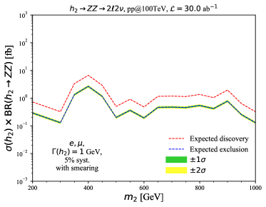
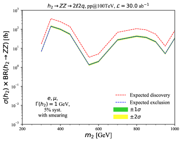
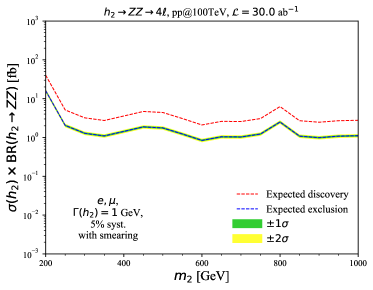
Figure 10: The expected discovery ($5\sigma$, red dashes) and exclusion ($2\sigma$, blue dashes) cross sections multiplied by the branching ratio of $h_{2}\rightarrow ZZ$, at a 100 TeV proton collider with an integrated luminosity of 30 ab^-1, coming from the three analyses $h_{2}\rightarrow ZZ\rightarrow 2\ell 2\nu$ (top left), $h_{2}\rightarrow ZZ\rightarrow 2\ell 2q$ (top right) and $h_{2}\rightarrow ZZ\rightarrow 4\ell$ (bottom). The expected $1\sigma$ and $2\sigma$ variation bands are shown for the expected exclusion.

To obtain the best limit on $\sigma(h_{2})\times\mathrm{BR}(h_{2}\rightarrow ZZ)$, we pick the most constraining analysis at each value of $m_{2}$. This is in fact represented by the $h_{2}\rightarrow ZZ\rightarrow(2\ell)(2\nu)$ analysis in the mass range we consider, as can be observed in fig. 10. A combination of the channels should yield a more stringent limit, but we omit it in the absence of a full study of the correlations between channels. Furthermore, the $(2\ell)(2q)$ and $4\ell$ final states will allow for reconstruction of the $h_{2}$ and therefore a precise determination of its mass in case of discovery.

F.1.3 pp@100 TeV $h_{2}\rightarrow W^{+}W^{-}$

For the analysis of the $W^{+}W^{-}$ final state we follow the ATLAS analysis of [131] focusing on the $WW\rightarrow(e\nu)(\mu\nu)$ final state. We require two oppositely-charged different-flavour leptons with transverse momenta $p_{T}(\ell_{1,2})>80,60$ GeV with combined invariant mass $m(\ell_{1}\ell_{2})>60$ GeV and maximum pseudo-rapidity difference $|\eta(\ell_{1})-\eta(\ell_{2})|$. We veto events that contain additional leptons with $p_{T}\geq 15$ GeV. To reject the backgrounds originating from $t\bar{t}$, we veto events containing $b$-jets with $p_{T}>30$ GeV. The $b$-jet tagging probability was chosen to be $0.75$. We also allow for the mis-identification of jets as leptons, with flat probability $5\times 10^{-3}$. For the events that pass the above constraints, we construct the transverse masses of the two $W_{i}$’s ($i=1,2$) as:

$$m_{T}^{W_{i}}=\sqrt{2p_{T}(\ell_{i})\not{p}_{T}(1-\cos(\phi^{\ell_{i}}-\not{\phi}))}\;,$$ (F.3)

where $p_{T}(\ell_{i})$ are the lepton transverse momenta, $\not{p}_{T}$ is the missing transverse momentum, $\phi^{\ell_{i}}$ and $\not{\phi}$ are the azimuthal angles of the lepton $i$ and the missing transverse momentum vector, respectively. We require both of these observables $i=1,2$ to satisfy $m_{T}^{W_{i}}>60$ GeV. We also construct an event transverse mass via:

$$m_{T}=\sqrt{(E_{T}(\ell\ell)+\not{p}_{T})^{2}-|\vec{p}_{T}(\ell\ell)+\vec{\not{p}}_{T}|^{2}}\;,$$ (F.4)

where the combined transverse energy of the leptons was defined as $E_{T}(\ell\ell)=\sqrt{|\vec{p}_{T}(\ell\ell)|^{2}+m(\ell\ell)^{2}}$.

The final set of observables consists of: $\bullet$ the lepton transverse momenta, $p_{T}(\ell_{1,2})$, $\bullet$ the di-lepton transverse momentum, $p_{T}(\ell\ell)$, $\bullet$ the di-lepton invariant mass $m(\ell\ell)$, $\bullet$ the distance between the leptons $\Delta R(\ell_{1},\ell_{2})$, $\bullet$ their pseudo-rapidity distance $\Delta\eta=|\eta(\ell_{1})-\eta(\ell_{2})|$, $\bullet$ the $W$ transverse masses $m_{T}^{W_{i}}$, $\bullet$ the event transverse mass, $m_{T}$, and $\bullet$ the magnitude of the missing transverse momentum, $\not{p}_{T}$. As background processes we have considered the SM $WW$, $t\bar{t}$, $ZZ$, $WZ$ processes, simulated at NLO via MC@NLO and the $W$+jets process simulated via FxFx merging at NLO.

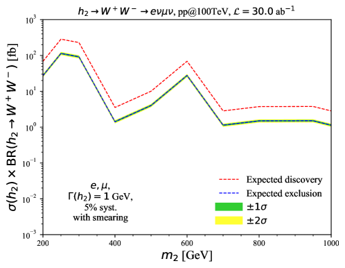
Figure 11: The expected discovery ($5\sigma$, red dashes) and exclusion ($2\sigma$, blue dashes) cross sections multiplied by the branching ratio of $h_{2}\rightarrow W^{+}W^{-}$, coming from the $h_{2}\rightarrow W^{+}W^{-}\rightarrow e\nu\mu\nu$ analysis, at a 100 TeV proton collider with an integrated luminosity of 30 ab^-1. The expected $1\sigma$ and $2\sigma$ variation bands are shown for the expected exclusion.

We show the resulting expected ($5\sigma$, red dashes) and exclusion ($2\sigma$, blue dashes) cross sections times branching ratio, $\sigma(h_{2})\times\mathrm{BR}(h_{2}\rightarrow W^{+}W^{-})$, in fig. 11. The constraints obtained through the $h_{2}\rightarrow W^{+}W^{-}\rightarrow e\nu\mu\nu$ are comparable to those coming from the $h_{2}\rightarrow ZZ$ analyses. These could be improved in future studies, e.g. by including hadronic decay modes of the $W$ bosons.

F.1.4 pp@100 TeV resonant Higgs boson pair production, $h_{2}\rightarrow h_{1}h_{1}$

The non-resonant $h_{1}h_{1}$ final state has been investigated at a 100 TeV collider in [157]. Here we investigate resonant $pp\rightarrow h_{2}\rightarrow h_{1}h_{1}$ production at 100 TeV. We focus on by far the most sensitive final state, $h_{1}h_{1}\rightarrow(b\bar{b})(\gamma\gamma)$. Future studies may include other final states to improve on this, see e.g. [158, 159, 160]. We require all jets (including $b$-tagged) to have transverse momentum $p_{T}>30$ GeV and to lie within $|\eta|<3.0$. The $b$-jet tagging probability was set to 0.75, uniform over the transverse momentum, as for the previous analysis. The jet to photon mis-identification probability was set to $0.01\times\exp{(p_{T}/30~{}\mathrm{GeV})}$, where $p_{T}$ is the jet transverse momentum [161]. We require that the invariant mass of the two $b$-jets lies in $m_{bb}\in[100,150]$ GeV and that the invariant mass of the di-photon system within $m_{\gamma\gamma}\in[115,135]$ GeV.

The final set of observables constructed for the BDT consists of: $\bullet$ the invariant mass of the two $b$-jets, $m_{bb}$, $\bullet$ the invariant mass of the di-photon system, $m_{\gamma\gamma}$, $\bullet$ the invariant mass of the combined system of the two $b$-jets and the photons, $m_{bb\gamma\gamma}$, $\bullet$ the distance between the $b$-jets, $\Delta R(b,b)$ $\bullet$ the distance between the photons, $\Delta R(\gamma\gamma)$, $\bullet$ the distance between the two $b$-jet system and the di-photon system, $\Delta R(bb,\gamma\gamma)$, $\bullet$ the transverse momentum of each $b$-jet, $p_{T}(b_{1},2)$, $\bullet$ the transverse momentum of each photon $p_{T}(\gamma_{1})$, $p_{T}(\gamma_{2})$, $\bullet$ the transverse momentum of the two $b$-jet system, $p_{T}(bb)$, $\bullet$ the transverse momentum of the di-photon system $p_{T}(\gamma\gamma)$, the transverse momentum of the combined $b$-jet and photon systems, $p_{T}(bb\gamma\gamma)$ and $\bullet$ the distances between any photon and any $b$-jet, $\Delta R(b_{i},\gamma_{j})$ with $i,j=1,2$. As backgrounds we consider $\gamma\gamma$+jets, $\gamma$+jets, by producing, respectively, $\gamma\gamma j$ and $\gamma jj$ via MC@NLO, $t\bar{t}\gamma\gamma$ via MC@NLO, $b\bar{b}\gamma\gamma$ and $bj\gamma\gamma$ at LO. We also consider backgrounds originating from single Higgs boson production: $b\bar{b}h_{1}$, $Zh_{1}$, $t\bar{t}h_{1}$, where we assume that the branching ratios possess their SM values. We also consider the non-resonant part of $h_{1}h_{1}$ as a background, assuming that the self-coupling maintains a value close to the SM value. In the case of discovery of a new scalar particle, the full interference pattern should be considered in a more detailed analysis. We leave this endeavour to future work.

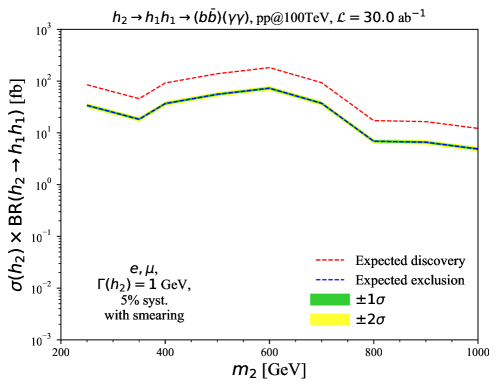
Figure 12: The expected discovery ($5\sigma$, red dashes) and exclusion ($2\sigma$, blue dashes) cross sections multiplied by the branching ratio of $h_{2}\rightarrow h_{1}h_{1}$, coming from the $h_{2}\rightarrow h_{1}h_{1}\rightarrow e\nu\mu\nu$ analysis, at a 100 TeV proton collider with an integrated luminosity of 30 ab^-1. The expected $1\sigma$ and $2\sigma$ variation bands are shown for the expected exclusion.

We show the expected discovery ($5\sigma$, red dashes) and exclusion ($2\sigma$, blue dashes) cross sections multiplied by the branching ratio of $h_{2}\rightarrow h_{1}h_{1}$ in fig. 12. The magnitude of the constraints is comparable to that of the gauge boson analyses. We note here that the same process was also considered in [52] in the context of the real singlet extension of the SM. Our results appear to be comparable but somewhat different. This can be attributed to differences in the analysis approach: we have calculated the $K$-factors for both signal and backgrounds, we have considered the vector-boson fusion process as part of the signal process as well as a different set of observables for which we ran the BDT. We also use the HERWIG Monte Carlo event generator, hence a completely different “tune” for the parton showering and the description of non-perturbative effects. We expect the aforementioned facts, in conjunction with different parton density functions for the incoming proton beams, that contain rather large uncertainties when extrapolated to higher energies, will introduce large differences in the significances, at the level observed between our results and the results of [52]. We expect all of these issues to be evaluated in detail at the onset of operation of any future collider through more precise phenomenological analyses.

F.2 Extrapolation of Heavy Higgs boson searches to 27 TeV

To obtain an estimate of the performance of a potential upgrade of the LHC to 27 TeV centre-of-mass energy, we consider an extrapolation of the detailed analyses obtained in the previous sections. We write the collider energy ($E$) dependence of the cross sections in the significance, given in Eq. F.1, as

$$\mathcal{S}(E,\mathcal{L})=\frac{\sigma_{S}(E)\mathcal{L}}{\sqrt{\sigma_{B}(E)\mathcal{L}+\alpha^{2}\sigma_{B}^{2}(E)\mathcal{L}^{2}}}\;.$$ (F.5)

To extrapolate the obtained limits through our detailed analyses to a different energy $E^{\prime}$ and luminosity $\mathcal{L}^{\prime}$, we solve Eq. F.1 for $\sigma_{S}(E^{\prime})$:

$$\sigma_{S}({E^{\prime}})=\frac{\mathcal{S}(E^{\prime},\mathcal{L}^{\prime})}{\mathcal{L}^{\prime}}\sqrt{\sigma_{B}(E^{\prime})\mathcal{L}+\alpha^{2}\sigma_{B}^{2}(E^{\prime})\mathcal{L}^{\prime 2}}\;.$$ (F.6)

Under the approximation that the impact of the analysis cuts remains the same between 100 TeV and 27 TeV, to obtain a limit on the signal cross section at the new energy $E^{\prime}$ we only need to determine the change in the total background cross section $\sigma_{B}(E)\rightarrow\sigma_{B}(E^{\prime})$ with energy. We achieve this by assuming that the background cross sections scale in the same way as either the $gg\rightarrow h_{2}$ process or a (hypothetical) $q\bar{q}\rightarrow h_{2}$ process. Since the analysis cuts will emphasise regions of phase space in which the backgrounds behave similarly to the signal, this should be a reasonable approximation. We assume that the $gg$ and $q\bar{q}$ scalings provide the error estimate on this part of our extrapolation. In the derivation of the actual limits, we use the one that provides the weakest signal constraints, so as to provide a conservative performance of a 27 TeV machine under this procedure. Another noteworthy assumption is that there will remain a sufficient number of signal events at 27 TeV after the analysis cuts are applied. This assumption ignores the fact that the extrapolation is performed from higher centre-of-mass energy and luminosity. This leads to potentially optimistic results and these should be assessed in a fully-fledged phenomenological analysis at 27 TeV.

The results for the 27 TeV extrapolation of the individual channels are shown in fig. 6. The $ZZ$ final state represents the highest significance all over parameter space as for the case of the 100 TeV collider.

Appendix G Results for the alternative categorisation of parameter-space points

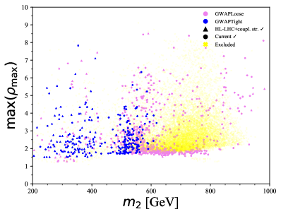
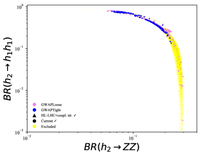
Figure 13: A selection of results for the “Tight” and “Loose” categorisations section 3.3. Left: The maximum value of $\rho_{\mathrm{max}}=\phi_{C}/T_{C}$ over the set of eight variations for each of the parameter-space points against the mass of $h_{2}$, $m_{2}$, right: The branching ratio of BR$(h_{2}\rightarrow h_{1}h_{1})$ plotted against BR$(h_{2}\rightarrow ZZ)$. We show points that pass the current constraints ($\CIRCLE$) or the HL-LHC constraints plus future signal strength ($|\sin\theta|<0.1$) constraints ($\blacktriangle$), as well as those that are currently excluded (faint $\color[rgb]{1,1,0}\boldsymbol{\times}\color[rgb]{0,0,0}$).

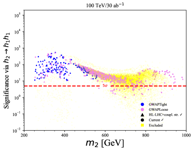
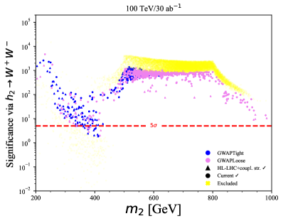
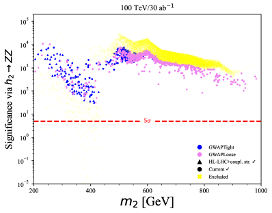
Figure 14: A selection of results for the “Tight” and “Loose” categorisations section 3.3. Top left: the statistical significance for a heavy Higgs boson ($h_{2}$) signal at a 100 TeV collider with an integrated luminosity corresponding to $30$ ab^-1 through $pp\rightarrow h_{2}\rightarrow h_{1}h_{1}$, top right: through $pp\rightarrow h_{2}\rightarrow W^{+}W^{-}$ and bottom: through $pp\rightarrow h_{2}\rightarrow ZZ$. We indicate the $5\sigma$ (discovery) boundaries by the red dashed lines. We show points that pass the current constraints ($\CIRCLE$) or the HL-LHC constraints plus future signal strength ($|\sin\theta|<0.1$) constraints ($\blacktriangle$), as well as those that are currently excluded (faint $\color[rgb]{1,1,0}\boldsymbol{\times}\color[rgb]{0,0,0}$).

Figures 13 and 14 present a selection of results for the alternative categorisation of “Tight” and “Loose” points described in section 3.3, found during the parameter-space scans via PhaseTracer. The results show that the “Centrist” and “Loose” categories behave in a similar fashion, whereas the “Liberal” category of the first classification has no correspondence in the second and allows for larger theoretical uncertainties.

Appendix H Fine-tuning studies

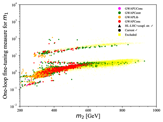
Figure 15: The value of the one-loop fine-tuning measure plotted against the one-loop mass of $h_{2}$, $m_{2}$. We show points that pass the current constraints ($\CIRCLE$) or the HL-LHC constraints plus future signal strength ($|\sin\theta|<0.1$) constraints ($\blacktriangle$), as well as those that are currently excluded (faint $\color[rgb]{1,1,0}\boldsymbol{\times}\color[rgb]{0,0,0}$).

Any parameter-space point has to contain a light Higgs boson, $h_{1}$, close enough to $125.1$ GeV, if it is to be phenomenologically relevant. It is therefore reasonable to investigate whether the introduction of additional interactions requires fine tuning of the parameters to achieve the observed Higgs boson mass. To do this, we employ the Barbieri-Giudice measure [162] (see also [163]):

$$\Delta=\max_{i,j}\left|\frac{\partial\log\mathcal{O}_{i}}{\partial\log p_{j}}\right|=\max_{i,j}\left|\frac{\mathcal{O}_{i}}{p_{j}}\frac{\partial\mathcal{O}_{i}}{\partial p_{j}}\right|\;,$$ (H.1)

for a set of observables $\mathcal{O}_{i}$ and a set of model parameters $p_{j}$. One can roughly interpret the logarithm of $\Delta$ as the number of significant digits that need to be tuned in at least one of the parameters of the theory.

We are interested in fine tuning in the Higgs boson mass and hence we consider derivatives of the one-loop expression for $\mathcal{O}=m_{1}$ with respect to the relevant free parameters in this case.

$$\Delta=\max_{j}\left|\frac{p_{j}}{m_{1}}\frac{\partial m_{1}}{\partial p_{j}}\right|\;.$$ (H.2)

We consider this quantity for each of the parameter-space points and plot against the one-loop value of $m_{2}$ at renormalisation scale $\mu=m_{Z}$. The derivatives have been calculated numerically.

The results are shown in fig. 15. It is evident that the parameter-space points that we consider do not possess substantial fine tuning. This is in line with the tree-level studies of ref. [163], where it was pointed out that it is possible to have a large hierarchy of scales in theories with extended Higgs sectors, without having fine tuning.

References

- [1] M.J. Ramsey-Musolf, The Electroweak Phase Transition: A Collider Target, 1912.07189.
- [2] C. Caprini et al., Detecting gravitational waves from cosmological phase transitions with LISA: an update, JCAP 03 (2020) 024 [1910.13125].
- [3] M. Benedikt, M. Capeans Garrido, F. Cerutti, B. Goddard, J. Gutleber, J.M. Jimenez et al., Future Circular Collider - European Strategy Update Documents, Tech. Rep. CERN-ACC-2019-0005, CERN, Geneva (Jan, 2019).
- [4] S. Sato, S. Kawamura, M. Ando, T. Nakamura, K. Tsubono, A. Araya et al., The status of DECIGO, Journal of Physics: Conference Series 840 (2017) 012010.
- [5] D.J. Weir, Gravitational waves from a first order electroweak phase transition: a brief review, Phil. Trans. Roy. Soc. Lond. A 376 (2018) 20170126 [1705.01783].
- [6] A. Mazumdar and G. White, Review of cosmic phase transitions: their significance and experimental signatures, Rept. Prog. Phys. 82 (2019) 076901 [1811.01948].
- [7] R. Zhou, L. Bian and H.-K. Guo, Connecting the electroweak sphaleron with gravitational waves, Phys. Rev. D 101 (2020) 091903 [1910.00234].
- [8] A. Kobakhidze, C. Lagger, A. Manning and J. Yue, Gravitational waves from a supercooled electroweak phase transition and their detection with pulsar timing arrays, Eur. Phys. J. C 77 (2017) 570 [1703.06552].
- [9] B. von Harling and G. Servant, QCD-induced Electroweak Phase Transition, JHEP 01 (2018) 159 [1711.11554].
- [10] A. Beniwal, M. Lewicki, M. White and A.G. Williams, Gravitational waves and electroweak baryogenesis in a global study of the extended scalar singlet model, JHEP 02 (2019) 183 [1810.02380].
- [11] M. Punturo et al., The Einstein Telescope: A third-generation gravitational wave observatory, Class. Quant. Grav. 27 (2010) 194002.
- [12] K. Kajantie, M. Laine, K. Rummukainen and M.E. Shaposhnikov, Is there a hot electroweak phase transition at m(H) larger or equal to m(W)?, Phys. Rev. Lett. 77 (1996) 2887 [hep-ph/9605288].
- [13] D.E. Morrissey and M.J. Ramsey-Musolf, Electroweak baryogenesis, New J. Phys. 14 (2012) 125003 [1206.2942].
- [14] G.A. White, A Pedagogical Introduction to Electroweak Baryogenesis, .
- [15] M. Pietroni, The Electroweak phase transition in a nonminimal supersymmetric model, Nucl. Phys. B 402 (1993) 27 [hep-ph/9207227].
- [16] J.M. Cline and P.-A. Lemieux, Electroweak phase transition in two Higgs doublet models, Phys. Rev. D 55 (1997) 3873 [hep-ph/9609240].
- [17] S.W. Ham, S.K. OH, C.M. Kim, E.J. Yoo and D. Son, Electroweak phase transition in a nonminimal supersymmetric model, Phys. Rev. D 70 (2004) 075001 [hep-ph/0406062].
- [18] K. Funakubo, S. Tao and F. Toyoda, Phase transitions in the NMSSM, Prog. Theor. Phys. 114 (2005) 369 [hep-ph/0501052].
- [19] V. Barger, P. Langacker, M. McCaskey, M. Ramsey-Musolf and G. Shaughnessy, Complex Singlet Extension of the Standard Model, Phys. Rev. D 79 (2009) 015018 [0811.0393].
- [20] D.J.H. Chung and A.J. Long, Electroweak Phase Transition in the munuSSM, Phys. Rev. D 81 (2010) 123531 [1004.0942].
- [21] J.R. Espinosa, T. Konstandin and F. Riva, Strong Electroweak Phase Transitions in the Standard Model with a Singlet, Nucl. Phys. B854 (2012) 592 [1107.5441].
- [22] T.A. Chowdhury, M. Nemevsek, G. Senjanovic and Y. Zhang, Dark Matter as the Trigger of Strong Electroweak Phase Transition, JCAP 02 (2012) 029 [1110.5334].
- [23] G. Gil, P. Chankowski and M. Krawczyk, Inert Dark Matter and Strong Electroweak Phase Transition, Phys. Lett. B 717 (2012) 396 [1207.0084].
- [24] M. Carena, G. Nardini, M. Quiros and C.E. Wagner, MSSM Electroweak Baryogenesis and LHC Data, JHEP 02 (2013) 001 [1207.6330].
- [25] J.M. No and M. Ramsey-Musolf, Probing the Higgs Portal at the LHC Through Resonant di-Higgs Production, Phys. Rev. D 89 (2014) 095031 [1310.6035].
- [26] G.C. Dorsch, S.J. Huber and J.M. No, A strong electroweak phase transition in the 2HDM after LHC8, JHEP 10 (2013) 029 [1305.6610].
- [27] D. Curtin, P. Meade and C.-T. Yu, Testing Electroweak Baryogenesis with Future Colliders, JHEP 11 (2014) 127 [1409.0005].
- [28] W. Huang, Z. Kang, J. Shu, P. Wu and J.M. Yang, New insights in the electroweak phase transition in the NMSSM, Phys. Rev. D 91 (2015) 025006 [1405.1152].
- [29] S. Profumo, M.J. Ramsey-Musolf, C.L. Wainwright and P. Winslow, Singlet-catalyzed electroweak phase transitions and precision Higgs boson studies, Phys. Rev. D 91 (2015) 035018 [1407.5342].
- [30] J. Kozaczuk, S. Profumo, L.S. Haskins and C.L. Wainwright, Cosmological Phase Transitions and their Properties in the NMSSM, JHEP 01 (2015) 144 [1407.4134].
- [31] M. Jiang, L. Bian, W. Huang and J. Shu, Impact of a complex singlet: Electroweak baryogenesis and dark matter, Phys. Rev. D 93 (2016) 065032 [1502.07574].
- [32] D. Curtin, P. Meade and H. Ramani, Thermal Resummation and Phase Transitions, Eur. Phys. J. C 78 (2018) 787 [1612.00466].
- [33] V. Vaskonen, Electroweak baryogenesis and gravitational waves from a real scalar singlet, Phys. Rev. D 95 (2017) 123515 [1611.02073].
- [34] G. Dorsch, S. Huber, T. Konstandin and J. No, A Second Higgs Doublet in the Early Universe: Baryogenesis and Gravitational Waves, JCAP 05 (2017) 052 [1611.05874].
- [35] P. Huang, A.J. Long and L.-T. Wang, Probing the Electroweak Phase Transition with Higgs Factories and Gravitational Waves, Phys. Rev. D 94 (2016) 075008 [1608.06619].
- [36] M. Chala, G. Nardini and I. Sobolev, Unified explanation for dark matter and electroweak baryogenesis with direct detection and gravitational wave signatures, Phys. Rev. D 94 (2016) 055006 [1605.08663].
- [37] P. Basler, M. Krause, M. Muhlleitner, J. Wittbrodt and A. Wlotzka, Strong First Order Electroweak Phase Transition in the CP-Conserving 2HDM Revisited, JHEP 02 (2017) 121 [1612.04086].
- [38] A. Beniwal, M. Lewicki, J.D. Wells, M. White and A.G. Williams, Gravitational wave, collider and dark matter signals from a scalar singlet electroweak baryogenesis, JHEP 08 (2017) 108 [1702.06124].
- [39] J. Bernon, L. Bian and Y. Jiang, A new insight into the phase transition in the early Universe with two Higgs doublets, JHEP 05 (2018) 151 [1712.08430].
- [40] G. Kurup and M. Perelstein, Dynamics of Electroweak Phase Transition In Singlet-Scalar Extension of the Standard Model, Phys. Rev. D 96 (2017) 015036 [1704.03381].
- [41] J.O. Andersen, T. Gorda, A. Helset, L. Niemi, T.V.I. Tenkanen, A. Tranberg et al., Nonperturbative Analysis of the Electroweak Phase Transition in the Two Higgs Doublet Model, Phys. Rev. Lett. 121 (2018) 191802 [1711.09849].
- [42] C.-W. Chiang, M.J. Ramsey-Musolf and E. Senaha, Standard Model with a Complex Scalar Singlet: Cosmological Implications and Theoretical Considerations, Phys. Rev. D 97 (2018) 015005 [1707.09960].
- [43] G.C. Dorsch, S.J. Huber, K. Mimasu and J.M. No, The Higgs Vacuum Uplifted: Revisiting the Electroweak Phase Transition with a Second Higgs Doublet, JHEP 12 (2017) 086 [1705.09186].
- [44] S. Bruggisser, B. Von Harling, O. Matsedonskyi and G. Servant, Electroweak Phase Transition and Baryogenesis in Composite Higgs Models, JHEP 12 (2018) 099 [1804.07314].
- [45] P. Athron, C. Balazs, A. Fowlie, G. Pozzo, G. White and Y. Zhang, Strong first-order phase transitions in the NMSSM — a comprehensive survey, JHEP 11 (2019) 151 [1908.11847].
- [46] K. Kainulainen, V. Keus, L. Niemi, K. Rummukainen, T.V.I. Tenkanen and V. Vaskonen, On the validity of perturbative studies of the electroweak phase transition in the Two Higgs Doublet model, JHEP 06 (2019) 075 [1904.01329].
- [47] L. Bian, Y. Wu and K.-P. Xie, Electroweak phase transition with composite Higgs models: calculability, gravitational waves and collider searches, JHEP 12 (2019) 028 [1909.02014].
- [48] H.-L. Li, M. Ramsey-Musolf and S. Willocq, Probing a Scalar Singlet-Catalyzed Electroweak Phase Transition with Resonant Di-Higgs Production in the Channel, 1906.05289.
- [49] C.-W. Chiang and B.-Q. Lu, First-order electroweak phase transition in a complex singlet model with symmetry, JHEP 07 (2020) 082 [1912.12634].
- [50] K.-P. Xie, Y. Wu and L. Bian, Electroweak baryogenesis and gravitational waves in a composite Higgs model with high dimensional fermion representations, 2005.13552.
- [51] N.F. Bell, M.J. Dolan, L.S. Friedrich, M.J. Ramsey-Musolf and R.R. Volkas, Two-Step Electroweak Symmetry-Breaking: Theory Meets Experiment, JHEP 05 (2020) 050 [2001.05335].
- [52] A.V. Kotwal, M.J. Ramsey-Musolf, J.M. No and P. Winslow, Singlet-catalyzed electroweak phase transitions in the 100 TeV frontier, Phys. Rev. D 94 (2016) 035022 [1605.06123].
- [53] T. Huang, J. No, L. Pernié, M. Ramsey-Musolf, A. Safonov, M. Spannowsky et al., Resonant di-Higgs boson production in the channel: Probing the electroweak phase transition at the LHC, Phys. Rev. D 96 (2017) 035007 [1701.04442].
- [54] C.-Y. Chen, J. Kozaczuk and I.M. Lewis, Non-resonant Collider Signatures of a Singlet-Driven Electroweak Phase Transition, JHEP 08 (2017) 096 [1704.05844].
- [55] A. Alves, T. Ghosh, H.-K. Guo and K. Sinha, Resonant Di-Higgs Production at Gravitational Wave Benchmarks: A Collider Study using Machine Learning, JHEP 12 (2018) 070 [1808.08974].
- [56] A. Alves, D. Gonçalves, T. Ghosh, H.-K. Guo and K. Sinha, Di-Higgs Production in the Channel and Gravitational Wave Complementarity, 1909.05268.
- [57] D. Croon, O. Gould, P. Schicho, T.V. Tenkanen and G. White, Theoretical uncertainties for cosmological first-order phase transitions, 2009.10080.
- [58] J. No and M. Spannowsky, Signs of heavy Higgs bosons at CLIC: An road to the Electroweak Phase Transition, Eur. Phys. J. C 79 (2019) 467 [1807.04284].
- [59] A. Alves, D. Gonçalves, T. Ghosh, H.-K. Guo and K. Sinha, Di-Higgs Blind Spots in Gravitational Wave Signals, 2007.15654.
- [60] D. Buttazzo, F. Sala and A. Tesi, Singlet-like Higgs bosons at present and future colliders, JHEP 11 (2015) 158 [1505.05488].
- [61] D. O’Connell, M.J. Ramsey-Musolf and M.B. Wise, Minimal Extension of the Standard Model Scalar Sector, Phys. Rev. D75 (2007) 037701 [hep-ph/0611014].
- [62] S. Profumo, M.J. Ramsey-Musolf and G. Shaughnessy, Singlet Higgs phenomenology and the electroweak phase transition, JHEP 08 (2007) 010 [0705.2425].
- [63] V. Barger, P. Langacker, M. McCaskey, M.J. Ramsey-Musolf and G. Shaughnessy, LHC Phenomenology of an Extended Standard Model with a Real Scalar Singlet, Phys. Rev. D77 (2008) 035005 [0706.4311].
- [64] G.M. Pruna and T. Robens, Higgs singlet extension parameter space in the light of the LHC discovery, Phys. Rev. D 88 (2013) 115012 [1303.1150].
- [65] C.-Y. Chen, S. Dawson and I.M. Lewis, Exploring resonant di-Higgs boson production in the Higgs singlet model, Phys. Rev. D91 (2015) 035015 [1410.5488].
- [66] T. Robens and T. Stefaniak, LHC Benchmark Scenarios for the Real Higgs Singlet Extension of the Standard Model, Eur. Phys. J. C 76 (2016) 268 [1601.07880].
- [67] C. Englert, J. Jaeckel, M. Spannowsky and P. Stylianou, Power meets Precision to explore the Symmetric Higgs Portal, Phys. Lett. B 806 (2020) 135526 [2002.07823].
- [68] S. Adhikari, I.M. Lewis and M. Sullivan, Beyond the Standard Model Effective Field Theory: The Singlet Extended Standard Model, 2003.10449.
- [69] J. Kozaczuk, M.J. Ramsey-Musolf and J. Shelton, Exotic Higgs boson decays and the electroweak phase transition, Phys. Rev. D 101 (2020) 115035 [1911.10210].
- [70] H.H. Patel and M.J. Ramsey-Musolf, Baryon Washout, Electroweak Phase Transition, and Perturbation Theory, JHEP 07 (2011) 029 [1101.4665].
- [71] A.D. Linde, Infrared Problem in Thermodynamics of the Yang-Mills Gas, Phys. Lett. 96B (1980) 289.
- [72] C.-W. Chiang, Y.-T. Li and E. Senaha, Revisiting electroweak phase transition in the standard model with a real singlet scalar, Phys. Lett. B 789 (2019) 154 [1808.01098].
- [73] P.B. Arnold and O. Espinosa, The Effective potential and first order phase transitions: Beyond leading-order, Phys. Rev. D47 (1993) 3546 [hep-ph/9212235].
- [74] T. Appelquist and R.D. Pisarski, High-Temperature Yang-Mills Theories and Three-Dimensional Quantum Chromodynamics, Phys. Rev. D23 (1981) 2305.
- [75] S. Nadkarni, Dimensional Reduction in Hot QCD, Phys. Rev. D27 (1983) 917.
- [76] M. Laine, Exact relation of lattice and continuum parameters in three-dimensional SU(2) + Higgs theories, Nucl. Phys. B 451 (1995) 484 [hep-lat/9504001].
- [77] K. Kajantie, M. Laine, K. Rummukainen and M.E. Shaposhnikov, Generic rules for high temperature dimensional reduction and their application to the standard model, Nucl. Phys. B458 (1996) 90 [hep-ph/9508379].
- [78] M. Karjalainen and J. Peisa, Dimensionally reduced U(1) + Higgs theory in the broken phase, Z. Phys. C 76 (1997) 319 [hep-lat/9607023].
- [79] M. Losada, High temperature dimensional reduction of the MSSM and other multiscalar models, Phys. Rev. D 56 (1997) 2893 [hep-ph/9605266].
- [80] J.M. Cline and K. Kainulainen, Supersymmetric electroweak phase transition: Dimensional reduction versus effective potential, Nucl. Phys. B 510 (1998) 88 [hep-ph/9705201].
- [81] J.O. Andersen, Dimensional reduction of the two Higgs doublet model at high temperature, Eur. Phys. J. C 11 (1999) 563 [hep-ph/9804280].
- [82] M. Laine and M. Losada, Two loop dimensional reduction and effective potential without temperature expansions, Nucl. Phys. B582 (2000) 277 [hep-ph/0003111].
- [83] M. Vepsalainen, Applications of dimensional reduction to electroweak and QCD matter, Ph.D. thesis, Helsinki U., 2007. 0709.2773.
- [84] T. Brauner, T.V.I. Tenkanen, A. Tranberg, A. Vuorinen and D.J. Weir, Dimensional reduction of the Standard Model coupled to a new singlet scalar field, JHEP 03 (2017) 007 [1609.06230].
- [85] T. Gorda, A. Helset, L. Niemi, T.V. Tenkanen and D.J. Weir, Three-dimensional effective theories for the two Higgs doublet model at high temperature, JHEP 02 (2019) 081 [1802.05056].
- [86] L. Niemi, H.H. Patel, M.J. Ramsey-Musolf, T.V. Tenkanen and D.J. Weir, Electroweak phase transition in the real triplet extension of the SM: Dimensional reduction, Phys. Rev. D 100 (2019) 035002 [1802.10500].
- [87] A. Andreassen, Gauge Dependence of the Quantum Field Theory Effective Potential, Master’s thesis, Norwegian U. Sci. Tech., 2013.
- [88] P.B. Arnold, Phase transition temperatures at next-to-leading order, Phys. Rev. D 46 (1992) 2628 [hep-ph/9204228].
- [89] M. Laine, The Two loop effective potential of the 3-d SU(2) Higgs model in a general covariant gauge, Phys. Lett. B335 (1994) 173 [hep-ph/9406268].
- [90] F. Staub, SARAH, 0806.0538.
- [91] P. Athron, C. Balázs, A. Fowlie and Y. Zhang, PhaseTracer: tracing cosmological phases and calculating transition properties, Eur. Phys. J. C 80 (2020) 567 [2003.02859].
- [92] C.L. Wainwright, CosmoTransitions: Computing Cosmological Phase Transition Temperatures and Bubble Profiles with Multiple Fields, Comput. Phys. Commun. 183 (2012) 2006 [1109.4189].
- [93] A. Fowlie, A fast C++ implementation of thermal functions, Comput. Phys. Commun. 228 (2018) 264 [1802.02720].
- [94] S. Baum, M. Carena, N.R. Shah, C.E. Wagner and Y. Wang, Nucleation is More than Critical – A Case Study of the Electroweak Phase Transition in the NMSSM, 2009.10743.
- [95] P. Bechtle, O. Brein, S. Heinemeyer, G. Weiglein and K.E. Williams, HiggsBounds: Confronting Arbitrary Higgs Sectors with Exclusion Bounds from LEP and the Tevatron, Comput. Phys. Commun. 181 (2010) 138 [0811.4169].
- [96] P. Bechtle, O. Brein, S. Heinemeyer, G. Weiglein and K.E. Williams, HiggsBounds 2.0.0: Confronting Neutral and Charged Higgs Sector Predictions with Exclusion Bounds from LEP and the Tevatron, Comput. Phys. Commun. 182 (2011) 2605 [1102.1898].
- [97] P. Bechtle, O. Brein, S. Heinemeyer, O. Stal, T. Stefaniak, G. Weiglein et al., Recent Developments in HiggsBounds and a Preview of HiggsSignals, PoS CHARGED2012 (2012) 024 [1301.2345].
- [98] P. Bechtle, S. Heinemeyer, O. Stal, T. Stefaniak and G. Weiglein, Applying Exclusion Likelihoods from LHC Searches to Extended Higgs Sectors, Eur. Phys. J. C 75 (2015) 421 [1507.06706].
- [99] P. Bechtle, S. Heinemeyer, O. Stål, T. Stefaniak and G. Weiglein, : Confronting arbitrary Higgs sectors with measurements at the Tevatron and the LHC, Eur. Phys. J. C 74 (2014) 2711 [1305.1933].
- [100] O. Stål and T. Stefaniak, Constraining extended Higgs sectors with HiggsSignals, PoS EPS-HEP2013 (2013) 314 [1310.4039].
- [101] P. Bechtle, S. Heinemeyer, O. Stål, T. Stefaniak and G. Weiglein, Probing the Standard Model with Higgs signal rates from the Tevatron, the LHC and a future ILC, JHEP 11 (2014) 039 [1403.1582].
- [102] FCC collaboration, FCC Physics Opportunities, Eur. Phys. J. C79 (2019) 474.
- [103] I.M. Lewis and M. Sullivan, Benchmarks for Double Higgs Production in the Singlet Extended Standard Model at the LHC, Phys. Rev. D 96 (2017) 035037 [1701.08774].
- [104] LHC Higgs Cross Section Working Group collaboration, Handbook of LHC Higgs Cross Sections: 4. Deciphering the Nature of the Higgs Sector, 1610.07922.
- [105] F. Dulat, A. Lazopoulos and B. Mistlberger, iHixs 2 — Inclusive Higgs cross sections, Comput. Phys. Commun. 233 (2018) 243 [1802.00827].
- [106] A. Papaefstathiou, G. Tetlalmatzi-Xolocotzi and M. Zaro, Triple Higgs boson production to six -jets at a 100 TeV proton collider, Eur. Phys. J. C 79 (2019) 947 [1909.09166].
- [107] ATLAS collaboration, Search for Higgs bosons produced via vector-boson fusion and decaying into bottom quark pairs in collisions with the ATLAS detector, Phys. Rev. D 98 (2018) 052003 [1807.08639].
- [108] ATLAS collaboration, Search for the standard model Higgs boson produced in association with top quarks and decaying into a pair in collisions at = 13 TeV with the ATLAS detector, Phys. Rev. D 97 (2018) 072016 [1712.08895].
- [109] ATLAS collaboration, Analysis of and production in multilepton final states with the ATLAS detector, .
- [110] CMS collaboration, Measurement of the associated production of a Higgs boson and a pair of top-antitop quarks with the Higgs boson decaying to two photons in proton-proton collisions at , .
- [111] CMS collaboration, Search for the Higgs boson decaying to two muons in proton-proton collisions at 13 TeV, Phys. Rev. Lett. 122 (2019) 021801 [1807.06325].
- [112] CMS collaboration, Evidence for the Higgs boson decay to a bottom quark–antiquark pair, Phys. Lett. B 780 (2018) 501 [1709.07497].
- [113] CMS collaboration, Inclusive search for a highly boosted Higgs boson decaying to a bottom quark-antiquark pair, Phys. Rev. Lett. 120 (2018) 071802 [1709.05543].
- [114] CMS collaboration, Measurement of production in the decay channel in of proton-proton collision data at , .
- [115] CMS collaboration, Evidence for associated production of a Higgs boson with a top quark pair in final states with electrons, muons, and hadronically decaying leptons at 13 TeV, JHEP 08 (2018) 066 [1803.05485].
- [116] CMS collaboration, Measurement of the associated production of a Higgs boson with a top quark pair in final states with electrons, muons and hadronically decaying leptons in data recorded in 2017 at , .
- [117] CMS Collaboration collaboration, Combination of standard model Higgs boson searches and measurements of the properties of the new boson with a mass near 125 GeV, Tech. Rep. CMS-PAS-HIG-12-045, CERN, Geneva (2012).
- [118] ATLAS collaboration, Combination of searches for heavy resonances decaying into bosonic and leptonic final states using 36 fb-1 of proton-proton collision data at TeV with the ATLAS detector, Phys. Rev. D 98 (2018) 052008 [1808.02380].
- [119] CMS Collaboration collaboration, Search for a new scalar resonance decaying to a pair of Z bosons in proton-proton collisions at = 13 TeV, Tech. Rep. CMS-PAS-HIG-17-012, CERN, Geneva (2017).
- [120] ATLAS collaboration, Combination of searches for Higgs boson pairs in collisions at 13 TeV with the ATLAS detector, Phys. Lett. B 800 (2020) 135103 [1906.02025].
- [121] CMS collaboration, Combination of searches for Higgs boson pair production in proton-proton collisions at 13 TeV, Phys. Rev. Lett. 122 (2019) 121803 [1811.09689].
- [122] ATLAS collaboration, Combined measurements of Higgs boson production and decay using up to fb-1 of proton-proton collision data at 13 TeV collected with the ATLAS experiment, Phys. Rev. D 101 (2020) 012002 [1909.02845].
- [123] CMS collaboration, Combined Higgs boson production and decay measurements with up to 137 fb-1 of proton-proton collision data at sqrts = 13 TeV, .
- [124] Projections for measurements of Higgs boson signal strengths and coupling parameters with the ATLAS detector at a HL-LHC, .
- [125] CMS collaboration, Sensitivity projections for Higgs boson properties measurements at the HL-LHC, .
- [126] HL/HE WG2 group collaboration, Higgs Physics at the HL-LHC and HE-LHC, 1902.00134.
- [127] CMS collaboration, Search for a new scalar resonance decaying to a pair of Z bosons in proton-proton collisions at TeV, JHEP 06 (2018) 127 [1804.01939].
- [128] P. Uwer, EasyNData: A Simple tool to extract numerical values from published plots, 0710.2896.
- [129] CMS collaboration, Search for a new scalar resonance decaying to a pair of Z bosons in proton-proton collisions at = 13 TeV, .
- [130] ATLAS collaboration, HL-LHC prospects for diboson resonance searches and electroweak vector boson scattering in the final state, .
- [131] ATLAS collaboration, Search for heavy resonances decaying into in the final state in collisions at TeV with the ATLAS detector, Eur. Phys. J. C 78 (2018) 24 [1710.01123].
- [132] K. Hagiwara, S. Matsumoto, D. Haidt and C. Kim, A Novel approach to confront electroweak data and theory, Z. Phys. C 64 (1994) 559 [hep-ph/9409380].
- [133] Gfitter Group collaboration, The global electroweak fit at NNLO and prospects for the LHC and ILC, Eur. Phys. J. C 74 (2014) 3046 [1407.3792].
- [134] J. Alwall, R. Frederix, S. Frixione, V. Hirschi, F. Maltoni, O. Mattelaer et al., The automated computation of tree-level and next-to-leading order differential cross sections, and their matching to parton shower simulations, JHEP 07 (2014) 079 [1405.0301].
- [135] V. Hirschi and O. Mattelaer, Automated event generation for loop-induced processes, JHEP 10 (2015) 146 [1507.00020].
- [136] R.D. Ball et al., Parton distributions with LHC data, Nucl. Phys. B867 (2013) 244 [1207.1303].
- [137] M. Bahr et al., Herwig++ Physics and Manual, Eur. Phys. J. C58 (2008) 639 [0803.0883].
- [138] S. Gieseke et al., Herwig++ 2.5 Release Note, 1102.1672.
- [139] K. Arnold et al., Herwig++ 2.6 Release Note, 1205.4902.
- [140] J. Bellm et al., Herwig++ 2.7 Release Note, 1310.6877.
- [141] J. Bellm et al., Herwig 7.0/Herwig++ 3.0 release note, Eur. Phys. J. C76 (2016) 196 [1512.01178].
- [142] J. Bellm et al., Herwig 7.1 Release Note, 1705.06919.
- [143] J. Bellm et al., Herwig 7.2 release note, Eur. Phys. J. C 80 (2020) 452 [1912.06509].
- [144] S. Frixione and B.R. Webber, Matching NLO QCD computations and parton shower simulations, JHEP 06 (2002) 029 [hep-ph/0204244].
- [145] R. Frederix and S. Frixione, Merging meets matching in MC@NLO, JHEP 12 (2012) 061 [1209.6215].
- [146] R. Frederix, S. Frixione, A. Papaefstathiou, S. Prestel and P. Torrielli, A study of multi-jet production in association with an electroweak vector boson, JHEP 02 (2016) 131 [1511.00847].
- [147] Papaefstathiou, Andreas, “The HwSim analysis package for HERWIG 7.”
- [148] R. Brun and F. Rademakers, ROOT: An object oriented data analysis framework, Nucl. Instrum. Meth. A389 (1997) 81.
- [149] M. Cacciari, G.P. Salam and G. Soyez, FastJet User Manual, Eur. Phys. J. C72 (2012) 1896 [1111.6097].
- [150] M. Cacciari, G.P. Salam and G. Soyez, The anti- jet clustering algorithm, JHEP 04 (2008) 063 [0802.1189].
- [151] ATLAS collaboration, Performance assumptions for an upgraded ATLAS detector at a High-Luminosity LHC, ATL-PHYS-PUB-2013-004 (2013) .
- [152] ATLAS collaboration, Performance assumptions based on full simulation for an upgraded ATLAS detector at a High-Luminosity LHC, ATL-PHYS-PUB-2013-009 (2013) .
- [153] P. Speckmayer, A. Hocker, J. Stelzer and H. Voss, The toolkit for multivariate data analysis, TMVA 4, J. Phys. Conf. Ser. 219 (2010) 032057.
- [154] S.D. Ellis, C.K. Vermilion and J.R. Walsh, Recombination Algorithms and Jet Substructure: Pruning as a Tool for Heavy Particle Searches, Phys. Rev. D 81 (2010) 094023 [0912.0033].
- [155] J. Thaler and K. Van Tilburg, Identifying Boosted Objects with N-subjettiness, JHEP 03 (2011) 015 [1011.2268].
- [156] R. Harlander, J. Klappert, C. Pandini and A. Papaefstathiou, Exploiting the WH/ZH symmetry in the search for New Physics, Eur. Phys. J. C 78 (2018) 760 [1804.02299].
- [157] M.L. Mangano, G. Ortona and M. Selvaggi, Measuring the Higgs self-coupling via Higgs-pair production at a 100 TeV p-p collider, 2004.03505.
- [158] A. Papaefstathiou, L.L. Yang and J. Zurita, Higgs boson pair production at the LHC in the channel, Phys. Rev. D87 (2013) 011301 [1209.1489].
- [159] D.E. Ferreira de Lima, A. Papaefstathiou and M. Spannowsky, Standard model Higgs boson pair production in the ( )( ) final state, JHEP 08 (2014) 030 [1404.7139].
- [160] A. Papaefstathiou, Discovering Higgs boson pair production through rare final states at a 100 TeV collider, Phys. Rev. D91 (2015) 113016 [1504.04621].
- [161] ATLAS Collaboration collaboration, Performance assumptions based on full simulation for an upgraded ATLAS detector at a High-Luminosity LHC, Tech. Rep. ATL-PHYS-PUB-2013-009, CERN, Geneva (Sep, 2013).
- [162] R. Barbieri and G. Giudice, Upper Bounds on Supersymmetric Particle Masses, Nucl. Phys. B 306 (1988) 63.
- [163] D. Boer, R. Peeters and S. Zeinstra, Analysis of fine-tuning measures in models with extended Higgs sectors, Nucl. Phys. B (2019) 114695 [1902.01258].