Cardea: An Open Automated Machine Learning Framework for Electronic Health Records

Abstract

An estimated 180 papers focusing on deep learning and EHR were published between 2010 and 2018. Despite the common workflow structure appearing in these publications, no trusted and verified software framework exists, forcing researchers to arduously repeat previous work. In this paper, we propose Cardea, an extensible open-source automated machine learning framework encapsulating common prediction problems in the health domain and allows users to build predictive models with their own data. This system relies on two components: Fast Healthcare Interoperability Resources (FHIR) – a standardized data structure for electronic health systems – and several AutoML frameworks for automated feature engineering, model selection, and tuning. We augment these components with an adaptive data assembler and comprehensive data- and model-auditing capabilities. We demonstrate our framework via 5 prediction tasks on Mimic-iii and Kaggle datasets, which highlight Cardea’s human competitiveness, flexibility in problem definition, extensive feature generation capability, adaptable automatic data assembler, and its usability.

I Introduction

Over the last decade, the number of data-driven machine learning models developed to tackle problems in healthcare has increased tremendously [1, 2]. Numerous studies have demonstrated machine learning’s effectiveness for predicting readmission rates, emergency room wait times, and the probability of a patient not showing up for an appointment [3, 4, 5].

However, a hospital or entity trying to build a model must start from scratch – a difficult process given that, at present, there is a significant shortage of data scientists with the requisite machine learning skills. Moreover, starting from scratch means retreading existing work: repeating essentially the same steps as previous studies, facing similar limitations and pitfalls, and re-engineering strategies to overcome them. Even worse, hospitals may complete this process only to find that gaps in data prevent their newly-built model from achieving the accuracy promised by the studies.

To address this complicated and troubling situation, we ask: “Could there be a simple way to share software that enables development of healthcare models more broadly?” Imagine this scenario: A user decides that s/he needs a model for predicting readmissions. S/he has access to a data engineer with programming and data management experience but not necessarily machine learning skills. The two of them access a community-driven, verified software platform to help develop a machine learning model from raw data. After two or three simple functional calls, they build a model and obtain numerous metrics, reports and recommendations. Such a workflow is the goal of our framework, which we call Cardea.

The integration of many sources of electronic health records via the wide scale adoption of the Fast Healthcare Interoperability Resources (FHIR) standardized format (schema) was intended to enable the development of reusable machine learning-based models [6, 7, 8, 9]. But while reusability was the original goal of the FHIR schema, the inevitable variance in the amount and quality of available data requires a framework that can adapt to missing tables and data items. In addition, the framework should be able to run the full prediction process using only available information.

Additionally, the past few years have seen the rise of automated approaches to machine learning model development. However, the construction of a powerful framework requires automation to work end-to-end: defining the initial prediction task, creating the features required for machine learning, and facilitating machine learning model development and tuning. Thus Cardea needed to define abstractions and intermediate data representations that allow the software to not be bound by intricacies specific to a particular data at hand.

Moreover, the system must be able to adapt to varying data availabilities and context-specific intricacies. For example, two hospitals with different subsets of tables and fields may spur an AutoML method to choose entirely different features and pipelines without manual intervention. The method must also allow users to tweak and extend predefined problems by adding functionality and/or modifying corresponding parameters. It should also enable advanced users to easily define and contribute new prediction problems, and allow the community to evaluate the contribution’s adherence to the abstractions.

In this paper, we present Cardea, an open-source framework for automatically creating predictive models from electronic healthcare data. Our contributions in this paper are:

• The first ever open-source, end-to-end automated machine learning framework for electronic healthcare data. .

• A set of key abstractions and data representations designed by carefully scrutinizing hundreds of machine learning studies on healthcare data. These abstractions allow us to transport data from its raw form to a predictive model while capturing metadata and statistics.

• An end-to-end framework incorporating an adaptive data assembler, an automated feature extractor, and an automated model tuning system.

• Through numerous case studies, we show the ability of the framework to adapt to different scenarios across multiple healthcare datasets. These datasets include Mimic-iii– an accessible, openly available and multi-purpose dataset – and the Kaggle dataset.

• Through case studies, we also present the framework’s competitiveness when compared with humans performance across many dimensions: model accuracy, reduction of software complexity, and ability to support numerous tasks humans can envision for the data.

The rest of this paper is organized as follows: We describe related work in the field in Section II, followed by the description of Cardea and its components in Section III. We demonstrate some use cases and their results in Sections IV & V. We report our user study in Section VI. Finally, Section VII presents discussion and Section VIII concludes the paper.

II Background and Related Work

II-A FHIR

There is a vast amount of literature proposing various standards for the electronic exchange of health information, most taking interoperability and integration as main objectives. Health Level 7 (HL7) introduced several of these standards in 1989; their first contribution is still used in over 90% of US hospitals [10].

Most recently, HL7 introduced FHIR, a new standard that aims to transcend the shortcomings of previous standards [11]. FHIR has been adopted across many technologies in the health industry, including mobile applications, prediction software, and health management systems. FHIR has been used to communicate patient information in addition to reporting prediction results [6]; for scalable development of deep learning models [7]; and to provide streamlined access to data for the development of mortality decision support applications [8]. Finally, FHIR standards are being integrated with several health management systems [9].

II-B Predictive Health Automation

The continuous collection of various patient data (demographics, lab tests, visits, procedures, drugs administered, etc.) [1] has driven an increase in the number of models and algorithms tackling health-related problems. Xiao et al. identified over 180 publications related to deep learning and EHR between 2010 and 2018.

The health-predictive models include: patient health prediction [12, 13, 14]; health-sector operations [15]; predicting patient mortality based on the competing risks that patients may experience over time [16]; and predicting the progression of Alzheimer’s in a patient [13]. In [14], the authors classify the severity of a radiology report based on the report’s textual features. The authors of [15] utilize insurance claim data to predict a patient’s length of stay.

In [17], the authors built a framework to identify survival risk factors. Their work demonstrates how automatic feature generation can surpass expert factors in performance. In addition, they highlight the impact of data-driven approaches in which they were able to deploy a machine learning model in $<1$ month, in comparison to the estimated 1-3 year development period. Computational Healthcare is another endeavor developed to analyze health data, generate statistics, and train and evaluate machine learning models [18]. However, although the tool is open-source and available online, it has not been updated over the past three years. Moreover, both frameworks support a limited number of prediction problems and are not generalizable across different data. They are instead tailored around a specific machine learning library, which limits their extensiblity.

III Cardea System

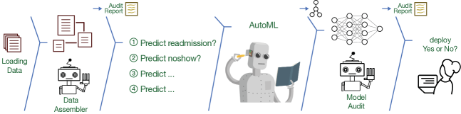
Figure 1: Cardea: A fully automated open-source framework for learning predictive models from electronic healthcare records. Cardea consists of multiple automated components. A automatic data assembler loads and organizes the data. A data-audit module automatically assesses the quality of different parts of the data. A set of prediction problems is stored in the library, allowing users to choose from them and set some of their parameters. An AutoML component generates and tunes training examples, features, labels, and models. A model-audit module appraises the resulting model along various metrics.

Cardea is an automated framework for building machine learning models from electronic health care records. Users first load their dataset into the framework through an adaptive data assembler. The data auditor generates a report that summarizes any discrepancies within the data. The user then selects a prediction problem to tackle from a list of predefined problems. Next, the framework starts the AutoML phase, which consists of three components: feature engineering, model selection, and hyperparameter tuning. Finally, the framework helps the user to audit the model’s results by reporting the model’s performance. Figure 1 depicts the framework’s workflow.

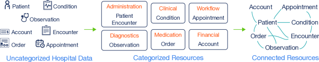
Figure 2: The FHIR standard can represent any health data in a categorized container format, which simplifies the exchange of data between connected resources. For example, $S^{p}$ (patient) and $S^{e}$ (encounter) fall under the administration module. $S^{c}$ (condition), which captures the health conditions for a patient, falls under the clinical module and is linked to the $S^{p}$.

III-A Adaptive Data Assembler

A typical healthcare dataset captures information about the various day-to-day aspects of a hospital, including administration, clinical records, drugs, and financial information. The extensive nature of this data creates a complex structure of intertwined information that could lead to disparate data organization schemas. FHIR is an international standard that helps to organize the exchange of hospital data [11]. Resources (tables), which are the basic building blocks in FHIR, define all exchangeable content for a particular resource, which then falls under a module, as shown in figure 2. In addition, possible connections with neighboring resources are preset in each resource’s metadata. The metadata identifying these relationships, table names, field names, and their types are available at: https://hl7.org/fhir/.

Notationally, for a given dataset, we have resources, $\mathcal{S}$, $S^{1..N}$, where each resource $S^{k}$ comprises variables $v_{1..j}$. We denote a variable $v_{j}\in S^{k}$ as $S^{k}_{j}$. To determine a relationship between $S^{1}$ and $S^{2}$ we form a dependence notation $S^{1}_{a}\rightarrow S^{2}_{b}$ which illustrates that $S^{1}$ holds a foreign key $v_{a}$ that references the primary key $v_{b}$ in $S^{2}$. This can be further simplified to $(S^{1}_{a},S^{2}_{b})\in\mathcal{R}$, where $\mathcal{R}$ is the set of all possible relations over $\mathcal{S}$. The structure is analogous to a directed graph $\mathcal{G}=\langle\mathcal{S},\mathcal{R}\rangle$ with vertices $\mathcal{S}$, and edges $\mathcal{R}$. Therefore, any data with an underlying relational database structure can be expressed in the framework as graph $\mathcal{G}$.

Although most standard schemata are comprehensive – for example, FHIR has a total of 492 resources with 2342 relational links – in almost all the scenarios we faced, we found that only a subset of the overall data was available to each hospital. Thus what data is available varies significantly. Therefore, as mentioned in Algorithm 1, an adaptive data assembler must accept any data $\mathcal{D}$ where $\mathcal{D}\subseteq\mathcal{S}$ and load $D^{k}_{a}$ into $S^{k}_{a}$ if $v_{a}\in D^{k}$ otherwise it continues to load the remaining $v_{b..j}\in D^{k}$; excluding nonexistent variables. Next, the algorithm tests loaded variables and adds possible relationships $\{(S^{k}_{i},S^{l}_{j})\;|\;\forall\;l\leq k\}$ s.t. $(S^{k}_{i},S^{l}_{j})\in\mathcal{R}$. In our current implementation, when a user uploads the data, the data assembler creates an in-memory representation (dictionary) of the metadata for only the resources loaded and relevant foreign keys, which we call an entityset $E$. In each iteration, the algorithm checks for a cycle graph in the relationships. If a conflict arises, the loader calls the function $\psi$($\cdot$, $\cdot$) to alter the structure of $E$ and $R$. The method receives any operation in which it consolidates the root resource with another and breaks the causing link in the least intrusive approach. Such a procedure is critical for adapting a metadata structure that conforms to the original schema, while resolving the challenges of foreign keys with missing primary keys.

Data: set of ingested data $\mathcal{D}$

Result: entityset $E$ of organized data, and relationships $R$

for $S^{k}\in\mathcal{S}$ do

       for $v_{i}\in S^{k}$ do

             if $v_{i}\in D^{k}$ then

                   $S^{k}\leftarrow S^{k}\cup D^{k}_{i}$

                   $R\leftarrow R\cup\{(S^{k}_{i},S^{l}_{j})\;|\;\forall\;l\leq k,(S^{k}_{i},S^{l}_{j})\in\mathcal{R}\}$

             else

                   $S^{k}\leftarrow S^{k}\cup\{\phi\}$

            

       end for

      $E(k)\leftarrow S^{k}$

       if $\exists\>(S^{1},\dots,S^{k})\in R\wedge S^{1}=S^{k}$ then

             $[E(k),R]\leftarrow\psi$($E$, $\bowtie$)

      

end for

return $E+R$;

Algorithm 1 Adaptive data assembler

III-B Specifying Prediction Problems

For most machine learning models, users define a specific outcome they would like to predict. They then prepare the data by identifying and generating labeled training examples along with time points for each training example. These time points separate the data that can be used to learn the model from the data that can’t be used. Authors in [19] note that this process underpins most prediction tasks across several domains; thus, formulating a prediction task and creating training examples can be further abstracted. Here is a breakdown of how Cardea undertakes these three steps:

Generating cutoff times: The cutoff time is a timestamp that splits the data into two segments: before and after. The data before the cutoff time is used to learn the model, while the data after is used for labeling. This is important because it ensures that predictive models are trained on data that does not already contain label information or other future information that is not usually available at the time of prediction, a problem widely known as label leakage. Cutoff times can be generated in several ways. In some cases, they are set based on the problem definition. For example, the cutoff time in a readmission problem is usually the time of discharge for each patient, whereas the cutoff time for a length of stay problem would be the time of admission. In Cardea, the method gct extracts pre-specified cutoff times, but the user also has the ability to overwrite the algorithm and create custom cutoff times. Figure 3 shows an example of a uniform cutoff time across several patients.

Writing a labeling function: Given a relational dataset, the cutoff time, and the target entity for which the prediction is sought, the labeling function $f(\cdot)$ is written to produce a label or target value.

Creating labeled training examples: Given a list of cutoff times for multiple entities, this method iterates over the cutoff times and generates labels for each entity-instance in the list.

After these three steps are complete, we have $\mathcal{X}$, what we call “label_times” - a tuple of $<e_{id}$, $t_{c}$, $l>$. With these label_times, the task of defining a prediction problem in Cardea is generalized. The problem definition is configured once, and it can be later stored and reused in the framework by any user. The procedure of these steps is detailed in Algorithm 2. For a given entityset $E$, and a target entity $E(k)$, the target label or outcome that one wants to predict may already exist as a column called target label $v_{l}$. Otherwise, a labeling function enables computation of the label for each entity instance. For every $e_{id}\in E(k)$ we specify a cutoff time $t_{c}$ as the start time or end time of an event + an offset (e.g. 24 hours) using gct, depending on the nature of the problem. To avoid label leakage, any event that occurs after that time will not be used to generate features.

Data: entityset $E$, target $k$, target label $v_{l}$

Result: set of tuples $\mathcal{X}$

Initialize $\mathcal{X}\leftarrow\{\phi\}$, offset $\epsilon$

for $e_{id}\in E(k)$ do

       $t_{c}\leftarrow$ gct($e_{id},\epsilon$)

       if $v_{l}\notin E(k)$ then

             $l\leftarrow f(E,t_{c},e_{id})$

            

       else

             $l\leftarrow v_{l}(e_{id})$

            

       $\mathcal{X}\leftarrow\mathcal{X}\cup{<e_{id},t_{c},l>}$

end for

return $\mathcal{X}$

Algorithm 2 Generating Label Times

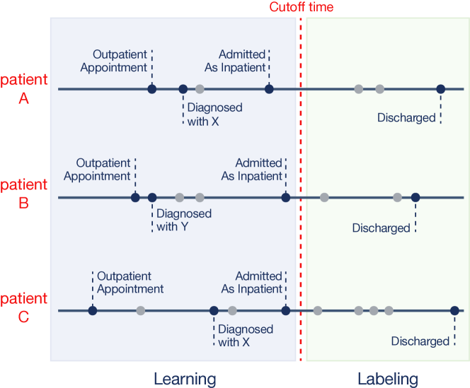
Figure 3: An example of cutoff time. Any events before a certain time are used for learning, while events after that time are used for labeling.

We present an initial list of predefined problems. These include predicting no-show appointments, length of stay, readmission, diagnosis prediction, and mortality prediction. This list will be expanded to include a broader set of prediction problems.

III-B1 Appointment No-Show

Predicting no-show appointments can help hospitals optimize their scheduling policies [4]. This problem is defined as a binary classification problem, as it predicts whether or not a patient will attend an appointment.

III-B2 Length of Stay

The system approaches this problem two ways: as a classification problem that determines which patients stayed more than a week from the point of admission [7], and as a regression problem that predicts the number of days a patient is expected to stay in a hospital [5].

III-B3 Readmission

Predicting patient readmission can help a hospital better manage its resources and measure its own performance and quality [20]. This is implemented as a binary classification prediction that predicts whether a patient will revisit the hospital within 30 days from the date of discharge [21].

III-B4 Diagnosis Prediction

Patient diagnosis prediction can help with the planning of intervention and care as well as with the optimization of resources [22]. The user provides a diagnosis code, and Cardea generates a target label according to whether the patient has received the specified diagnosis since the point of admission.

III-B5 Mortality Prediction

Hospital performance can be measured by predicting mortality as a performance indicator [23]. In the case where the mortality label is not present, the framework extracts this information through a list of underlying causes of death according to the visits’ diagnosis code, which includes motor vehicle accidents, intentional self-harm (suicide) and assault (homicide), then generates a target label based on this list of codes. Cardea treats this as a classification problem where it predicts patient mortality from the point of admission.

III-C Auto Machine Learning

Data scientists typically follow a fairly similar procedure for prediction problems. This repetitive effort motivated the automation of the machine learning workflow (e.g., [24, 25, 26]), which includes two main phases: first, the featurization of data, and second, modeling and tuning hyperparameters.

III-C1 Feature Engineering

Cardea utilizes the relational nature of the entityset $E$ to perform feature synthesis [27]. We use automated feature engineering tool called featuretools. Given an entityset, for each entry, corresponding to the entity instance $e_{id}$ in label_times, featuretools automatically performs two steps:

• Removes the data past the corresponding $t_{c}$ for that entry.

• Computes a rich set of features by aggregating and transforming data across all the entities. This is accomplished by executing an algorithm called Deep Feature Synthesis. For more details we refer the reader to [27] and the Featuretools library itself available at: https://github.com/FeatureLabs/featuretools.

Users can control the type of features and the number of features generated by Featuretools through specifying hyperparameters - such as aggregation primitives, depth, etc. The output of the feature engineering is a matrix of each entry $e_{id}$ with its engineered features. We combine the features generated with the labels extracted in algorithm 2 to obtain a dataset that is perfectly formatted for the succeeding component.

III-C2 Modeling and Hyperparameter Tuning

Considering the copious amount of machine learning algorithm libraries (e.g., scikit-learn, Tensorflow, Keras, and their AutoML versions), we opted to give the user the flexibility and freedom of using the library of their choice. We are able to accommodate for this dynamic structure while maintaining an interpretable format by using primitives and computational graphs as proposed in [28]. The user specifies the preprocessing, postprocessing, and ML algorithm s/he is interested in. In addition, we use Bayesian optimization methods to tune the hyperparameters [29]. This method aims to find optimal hyperparameters in fewer iterations by evaluating those that appear more promising based on past results (informed search). It achieves a better performance than random search or grid search [30, 31, 32, 33, 34].

IV Experimental Settings

In this section, we describe the characteristics of datasets loaded into Cardea, elaborate on the prediction tasks selected, and detail the settings used for the AutoML phase.

Datasets: To emphasize Cardea’s adaptivity to complex datasets, variability in data availability, and disparate prediction problems, we utilize two publicly available, widely studied complex datasets. To qualify as realistic, datasets have to be multi-table, with multiple entities, and complex. with several foreign key relationships. We used two datasets. The first, Kaggle’s Medical Appointment No-Shows dataset  [35], consists of 21 variables that were loaded into Cardea ’s data assembler to generate a total of 9 resources conforming to the FHIR structure. Kaggle contains an approximate 20:80 class division across patients that showed up to their appointments vs. not. The second, Mimic-iii, is a rich Electronic Health Records (EHR) dataset widely used in the research community to perform various prediction tasks. Overall, the data is composed of 40 tables, storing 534 variables and 63 relationships. (see appendix -B for complete description).

Prediction problem definitions: For Kaggle, we predict whether a patient will show up to an appointment. On the other hand, Mimic-iii includes both patient- and operations-centric information. Mimic-iii’s versatiliity allows us to test Cardea on a number of different prediction problems, including mortality, readmission, and length of stay.

AutoML Settings: AutoML is divided into two main components: first, feature engineering; second, modeling and hyperparameter tuning. For feature engineering, we apply central tendency and distribution operations $\oplus=\{$sum, standard deviation, max, min, skew, mean, count, and mode$\}$. In addition, we utilize time-oriented functions that extract day, month, year, and type of day (weekend/weekday). Maximum depth for extracting features is set to $N=2$. For preprocessing, we employ simple imputation and min-max scalers to normalize the data between [0, 1]. For modeling, we utilize eight classification methods and seven regression methods. (see appendix -C for full results). Moreover, each machine learning algorithm has a set of tunable hyperparameters used for Bayesian optimization of the model [29].

V Case studies

Our framework proposes a number of abstractions and data representations, and a set of automated tools, aimed at enabling the wide-scale use of machine learning to work with electronic healthcare records. In addition to performing competitively compared to a human, the framework should be adaptable, flexible across use cases, and easy to work with, and should reduce the need for extensive software re-engineering. In the following subsections, through a series of case studies, we demonstrate Cardea’s efficacy along these lines.

V-A Case study: Human competitiveness

Figure 4: Accuracy scores of Kaggle participants. The blue dotted lines indicate where Cardea was able to achieve an equivalent accuracy.

In this subsection, we showcase the results obtained by Cardea on Kaggle’s Medical Appointment No-Shows dataset and compare it to 78 kernel notebooks from [35] with their reported accuracy for the same prediction problem. One challenge is that individual users choose train-test splits, cross-validate, and report metrics differently. For a fair comparison with our classifiers, we report the average result over several cross-validation rounds. Figure 4 compares the framework to other users’ models at each percentile. Overall, Cardea performed well compared to the human users. More specifically, the Gradient Boosting Classifier (GB), which had an accuracy of 0.91, was able to score higher than 90% of kernel notebooks. Running the framework end-to-end automatically generates 95 features, which feed an ML pipeline that will likely outperform 80% of existing models.

V-B Case study: Flexibility and coverage

One of Cardea’s claims is that its abstractions support the formulation of any prediction problem on a healthcare dataset. To support this claim, we examine the Mimic-iii dataset, which is popular among researchers for modeling prediction tasks in healthcare. (As of writing this paper, there are 1,278 citations of the Mimic-iii dataset.) We surveyed a collection of 186 papers that applied machine learning to the Mimic-iii between 2017 and 2019; of those, 90 of them had prediction tasks. For each of these papers, we recorded (1) the prediction task it was trying to solve, (2) the data used, and (3) the label source of the data. Typically, authors combine multiple data sources to formulate a prediction problem. We summarize the prediction task information in Table I, where: $p_{1}$ is predicting patient mortality; $p_{2}$ is patient length of stay; $p_{3}$ is readmission; $p_{4}$ is ICD-9 code; $p_{5}$ is the treatment of a patient; and $p_{+}$ refers to the remaining problems. Note that $p_{1-3}$ are fully available in Cardea.

	Cardea			External
	$p_{1}$	$p_{2}$	$p_{3}$	$p_{4}$	$p_{5}$	$p_{+}$	Total
Tabular	19	6	3	7	6	8	49
Time series	6	1	0	1	1	13	22
Unstructured	5	0	1	15	3	7	31
Total	30	7	4	23	10	28	102*

• Papers targeting multiple prediction problems / using multiple data structures are counted separately.

TABLE I: Mimic-iii Surveyed Papers Summary.

Observing Table I, we notice that $\sim 30\%$ of the papers tackled the same prediction task ($p_{1}$, patient mortality). Given the copious number of prediction problems, we wondered why a generalized framework for reducing repetitive tasks does not exist. As presented in section III-B, we believe we can systematically abstract the problem definition task without losing each model’s nuances. To test our abstraction, we further examined all papers related to $p_{1}$ to understand how they can be formulated in Cardea.

Figure 5 depicts the breakdown of models that solve $p_{1}$. Viewing the plot from left to right, we first select entityset components: the target label $v_{l}$ and the entity of concern $k$. Next, we identify time-sensitive formulations through $t_{c}$ and $\epsilon$. For example, one of the most common formulations is predicting patient mortality after 48 hours of admission. In this case, our reference point $t_{c}$ is set to the time of admission and the offset for learning is $\epsilon=48$ hours. We discovered that each rendition of $p_{1}$ surveyed fit our proposed abstraction.

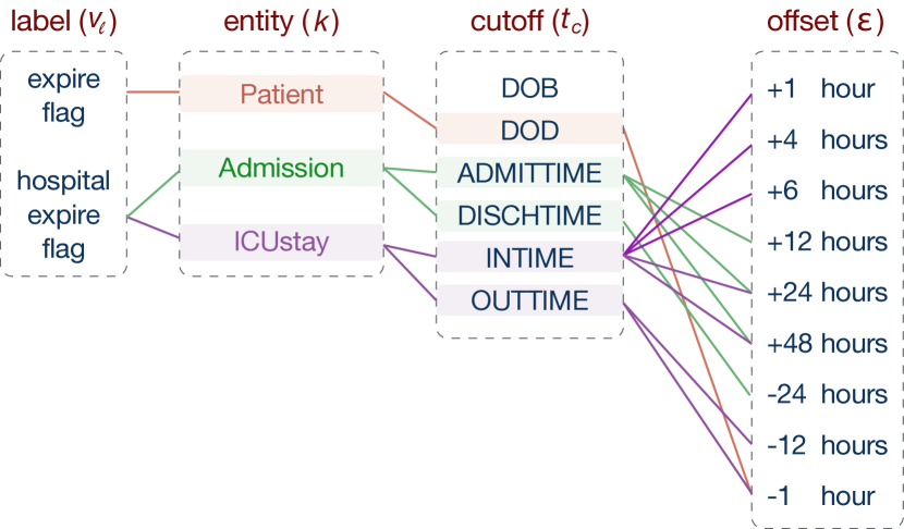
Figure 5: Breakdown of mortality prediction. The enclosing box details how Cardea’s abstraction can articulate all mortality prediction problems presented. The edges showcase all combinations present in $p_{1}$.

V-C Case study: Adaptivity

	MIMIC-Extract + AutoML			Cardea
	$\mu$ $\pm$ $\sigma$	best	best CL	$\mu$ $\pm$ $\sigma$	best	best CL
Mortality	0.540 $\pm$ 0.1643	0.740	LR	0.566 $\pm$ 0.0529	0.660	XGB
Readmission	0.459 $\pm$ 0.1455	0.540	SGD	0.540 $\pm$ 0.0628	0.635	XGB
LOS $\geq$ 7	0.560 $\pm$ 0.1296	0.691	GB	0.519 $\pm$ 0.1650	0.789	LR

TABLE II: Comparison of F1 Macro scores for models whose features were generated by classical approaches (MIMIC-Extract) and models whose features were generated automatically (Cardea)

After defining a widely accepted schema, one possible alternative is to write software for the rest of the process: data assembly, manipulation, pre-processing, and feature engineering. This approach was recently proposed by Wang et al., 2019 for the Mimic-iii database. Their tool, MIMIC-Extract, standardized this process and produced a structured input for widely known prediction tasks - mortality and length of stay [36] - the idea being that other users can exploit this software as long as their data follows the same schema. In addition to requiring subject matter experts with data science expertise to write software, this approach requires significant software maintenance. For instance, What if a new user only has data corresponding to a certain subset of tables? What if the original schema is updated over time? Software that is hard-coded can be brittle and would need consistent updates. Over time, this process would inevitably lead to large technical debt.

In this case study, we ask whether Cardea can help mitigate these two situations. Can Cardea’s automated submodules for feature engineering and data assembly do away with extensive hard-coded software engineering? Can it do so while maintaining competitiveness against experts? Even if automation creates competitive solutions, are they expressive?

Reducing the need for extensive software (re)engineering: MIMIC-Extract extracts 8 tables from the Mimic-iii database to prepare data for processing. Over 1,000 lines of code were written for the sole purpose of data structuring and featurization. We ask, how can more data from Mimic-iii be utilized? Can features other than the ones intended be used?

Our proposed framework adapts the entityset to any subschema available, thereby enabling the ingestion of any data type. Moreover, we use automated feature engineering. Figure 6 shows the distribution of correlations between expert-generated features and the most correlated feature from automated feature engineering. Cardea was able to extract a high proportion of features correlated to MIMIC-Extract. Cardea also generated features that were not in MIMIC-Extract: Cardea generated a total of  400 features, while the latter generated 180 features. The median correlation value is 0.39, 0.54, and 0.35 for the mortality, readmission, and length of stay features, respectively. What are these features, and how significant are they? To investigate this more deeply, we examined the important features (generated using the Random Forest (RF) classifier) which showed that Cardea relies on variables fetched from different sources, including the number of times the patient was previously diagnosed, the type of admission, and the number of conducted lab tests, which were fetched from the diagnosis, admission, and labevents tables respectively. On the other hand, the MIMIC-Extract approach focused on utilizing patient readings such as the Glasgow Coma Scale, lactic acid measurements, and arterial pH mean values, which all trace back to the chartevents table.

Figure 6: Histogram of feature correlation using Pearson’s correlation coefficient between expert-identified features through MIMIC-Extract and automatic feature generation by Cardea

Adapting to data availability The automation in Cardea not only eliminates the need for meticulously engineering features, it also allows for taking advantage of all the data at hand. But why is more data useful? Are the tables referred to by MIMIC-Extract only the important ones? To examine this further, we fed Cardea the same tables as MIMIC-Extract, set it as our baseline, and introduced more tables. From figure 7, we can see that in certain prediction problems the introduction of more tables improves the model’s performance - specifically in the LOS prediction. The best model was able to increase in performance from $0.61$ to $0.74$ (a 21% improvement). A huge performance increase happened at $x=6$, as table procedureevents was introduced, which is not included in the MIMIC-Extract pipeline. But how does the performance of Cardea compare to MIMIC-Extract?

Table II summarizes the results obtained from applying AutoML to features that were automatically generated by Cardea versus MIMIC-Extract, which we consider to exemplify a classical approach to making a prediction model. While MIMIC-Extract’s approach surpasses Cardea in mortality prediction by 12%, the latter triumphs in the other two problems. Moreover, in comparison to the other classifiers we tested, (see appendix -C for all classifiers), Cardea had a more consistent predictive accuracy, indicating that the features it considered are more telling. Overall, Cardea showed competitiveness and an ability to extract useful features from any shaped dataset.

Figure 7: The score of the model as we add more data tables. The line represents the smoothed curve of the best-performing classifier.

VI User Study

We conducted a user study to evaluate Cardea from different angles and to answer the following questions: (R1) Can users understand the concepts and functions of Cardea quickly and correctly? (R2) How effective is Cardea in supporting medical data analysis? and (R3) How do users perceive the usefulness of Cardea?

We held a 90-minute workshop with 10 participants, 7 males and 3 females, each having between 4 and 12 years of coding experience ($\mu$=7.7, $\sigma$=2.53) and between 2 and 5 years of machine learning experience ($\mu$=4.0, $\sigma$=1.10). The participants included graduate students, data analysts, researchers, and engineers. They are general users whose daily work involves data analysis, but they are not experts in analyzing medical data.

VI-A Tasks and Procedure

We started the workshop with a 30-minute tutorial+demo session, introducing the relevant background knowledge and demonstrating how to use Cardea. Next, we set up an one-hour quiz. We created our study datasets based on the Mimic-iii Demo data . The sampled data contains the same tables as the complete dataset, but the number of patients is reduced to 100.

The quiz required the participants to use Cardea to perform four tasks. Task 1 asked the participants to use Cardea  to load a specified dataset and observe the loaded tables. Task 2 asked the participants to explore potential prediction problems and then use Cardea to explore the predefined problems. Task 3 required the participants to use Cardea  to generate the feature matrix and prepare training and testing data for later use. Task 4 requested the participants to explore different pipelines and report the accuracy scores of the obtained models. To investigate whether users can effectively understand and use Cardea  (R1), after every task, the participants were asked several questions (Table III). We recorded the task accuracy and completion time. We also asked the participants to estimate what the completion time sould be without Cardea (R2). Four options ($<10$ minutes, $<1$ hour, $<3$ hours, and $\geq 3$ hours) were given, and we used $5$, $35$, $120$, and $180$ respectively as the actual estimated times in order to compute the average time.

At the end of the quiz, to get a more comprehensive understanding of Cardea ’s usefulness (R3), we asked the participants to fill out a survey to rate Cardea. We used 5-point Likert-scale questions with 1 being ”strongly disagree” and 5 being ”strongly agree.” The questions covered ease of use, ease of learning, effectiveness in solving medical data prediction problems, satisfaction, and utility (i.e., whether it provides all the features you need.).

Task	Question	Accuracy	Completion Time
			Cardea (min)	Estimated (min)	Speedup Times ($\simeq$x)
T1	Q1. How many entries were in the ”icustays” table? Q2. Is it helpful to display the ”relationship” of the entityset?	100%	4.86 (2.25)	57.50 (57.54)	12
T2	Q3. Given the data, can we predict a patient’s ICU time? Q4. Given the data, what is your prediction problem? Q5. Does your prediction problem already exist in Cardea?	70%	5.77 (2.11)	40.00 (42.19)	7
T3	Q6. How many features were generated? Q7. What is the datatype of y?	80% 100%	4.45 (0.84)	121.5 (67.57)	27
T4	Q8. Can you get a model with accuracy > 80%? Q9. What was the best accuracy score you obtained?	100%	4.25 (3.77)	55.63 (51.20)	13

TABLE III: Experimental tasks, questions, and results. Tasks are categorized into four classes corresponding to Cardea’s 4 components: data assembler (T1), problem definer (T2), featurizer (T3), and ML pipelines (T4). Task completion time is shown in Avg. (SD). The speedup times of every task are reported.

Ratings on	Mean	SD
Ease of use	4.2	0.6
Ease of learning	4.1	0.7
Effectiveness (in medical data predictive analysis)	4.2	0.87
Satisfaction	4.2	0.75
Utility (cover all desired features)	3.8	0.87

TABLE IV: Ratings on the overall experience on Cardea (1 $=$ strongly disagree, 2 $=$ disagree, 3 $=$ neutral, 4 $=$ agree, 5 $=$ strongly agree).

VI-B Result Analysis

Quiz results—task accuracy Table III summarizes the quiz results. We observed that all of the participants were able to answer the three questions (Q1, Q7, and Q8) related to data assembler (T1), featurizer (T3), and ML pipelines (T4), respectively. However, a few participants still failed to answer Q3 (with T2—problem definer; acc$=70\%$, 7/10) and Q6 (with T3—featurizer; acc$=80\%$, 8/10). This indicates that the participants had a good understanding of how data were loaded, transformed (y labels) and fed for training predictive models. Three participants (1 No and 2 Not sure) had difficulty judging whether a prediction problem was feasible given the data. This further motivated us to automatically provide a comprehensive prediction problem list. We also found that two participants had difficulty in understanding the feature matrix (Q6).

We asked several other questions to collect feedback from the participants, including Q2, Q4, Q5, and Q9. For Q2, the participants rated helpfulness on a 5-point Likert-scale score ($\mu$=4.0, $\sigma$=1.00). The prevailing score, 4, suggested that most people (70%, 7/10) thought this feature very helpful. For both Q4 and Q5, our purpose was to investigate whether our predefined problem list could satisfy user demands. The results reported that 4 out of 10 (40%) participants found their target prediction problems existed in Cardea, while the rest thought of a question outside. For Q9, the average accuracy is 89.8%, with the standard deviation being 4.30%, which suggests that the participants were able to try different pipelines to run the experiments. We further noted that one participant obtained 100% accuracy, which was possible as the experiments were run on a sampled dataset.

Quiz results—task completion time. From table III, we found that using Cardea  can significantly improve the efficiency of performing each type of task. The speedup time ranged from 7 to 27, where T3 (featurizer) had the largest efficiency increase (27x). On average, tasks regarding the types were expected to be completed in around 4 to 6 minutes using Cardea. T2 ($\mu$=5.77 min, $\sigma$=2.11) took the longest; this could be because participants had to spend time observing the metadata and investigating the problems. Although T4 ($\mu$=4.25 min, $\sigma$=3.77) had the least completion time, its SD was the highest. This can be explained by the fact that users can generally use Cardea  to learn a model in a short time, and the time a user spent depends on his/her expectation regarding performance.

Survey results—usability. Overall, as shown in Table IV, we received good feedback from the participants. Most participants agree or strongly agree that Cardea  is easy to use (9/10, $\mu$=4.2, $\sigma$=0.6), easy to learn (8/10, $\mu$=4.1, $\sigma$=0.7), and able to significantly improve their efficiency to perform prediction tasks (7/10, $\mu$=4.2, $\sigma$=0.87). Few participants held neutral options on these three aspects, which confirmed with our quiz results that few participants had difficulty in identifying proper prediction problems and understanding the auto-featurization process. Nearly all participants (8/10, $\mu$=4.2, $\sigma$=0.75) felt satisfied with the presented tool. Compared with the other four, the “utility” was scored relatively lower ($\mu$=3.8, $\sigma$=0.87), suggesting the absence of some user-desired features. The concerns lay mainly in two aspects: visual interface and controllability. One participant pointed out that a friendly visual interface would make Cardea  accessible to a wider audience. As for the controllability, one critic was concerned about high automation partly limiting users’ ability to explore freely.

VII Further Discussion

Cardea takes AutoML to the next level by engineering components that allow for flexible data ingestion, problem selection, and data- and model-understanding. In this section, we shed light on some of the more interesting findings from the results obtained in section V.

Adaptivity of Automatic Data Assembler: Most publicly available EHR datasets involve minimal, non-sensitive information about patients, and do not represent real scenarios. Therefore, we needed to test the robustness of the automatic data assembler. For this, we randomly sampled 100 subsets of Mimic-iii and fed it to the framework. In all cases, the framework adapts to the dimensions of the data and seamlessly proceeds to the next components.

Acceleration in Building Prediction Models: We conduct another experiment where we try to solve a new problem; predicting the risk of acquiring a certain disease [37]. We utilize a large dataset of $1.1$ million encounter records from a private EHR entity. The dataset is composed of 10 separate hospital records that were merged together. Using Cardea, not only were they able to run the framework from raw data to deployable models, but they achieved this result in $<1$ month.

Model Interpretation: The data- and model-auditor supplement the user with vital information describing the model. Continuing on the same real-world application mentioned, we leveraged the property of auditing into understanding the characteristics of the data. For example, out of the collection of 10 hospitals, we noticed that $hospital_{1}$ performed better than $hospital_{2}$, because the patient cohort in $hospital_{1}$ is less diverse than in $hospital_{2}$, decreasing the variance of the training data [38].

VIII Concluding Remarks

In this paper, we introduced Cardea, an open framework for creating healthcare prediction models automatically. In Cardea, we adopt HL7’s FHIR standard as an interface for representing data, and provide an abstraction for defining prediction problems, a set of coded prediction problems, and multiple modeling approaches. Through the proposed design, users overcome the limitations of manual feature engineering and single-model application, and are not limited to one prediction problem. While automation allows for scaling the number of prediction problems and hospitals that we can address without much manual effort, it also allows us to focus on developing a comprehensive systematic approach for assessing data and models. We demonstrated the efficacy of this framework by solving 5 prediction problems, comparing its performance to existing models, and evaluating the usability by a user study.

-A Auditing

-A1 Data Auditor

Data from different hospitals will inevitably have variations even if they conform to a standardized schema. These variations stem from hospitals’ differing execution of health management systems, resulting, for example, in missing values for certain fields; serving different populations. We most commonly encountered lack of demographic variables and diagnosis information; data from different and/or short time periods (temporal coverage); data from different geographical areas (spatial coverage); and general quality issues (inaccuracy, incompleteness, format inconsistency, etc.).

In a typical data science endeavor, data scientists summarize these caveats; while they don’t preclude the building of a predictive model, they do affect the model’s accuracy. For example, imagine a prediction problem for which age is an important feature. A dataset with incomplete age-related data will reduce the overall accuracy of the model. These issues should be reported in a systematic fashion, enabling the user to debug and ultimately trust the models. To address this, we created a data auditor. The data auditor uses a dictionary of checks for different fields and generates a data summary report. These checks are divided into two categories: data quality metrics and distribution checks.

Data quality metrics: calculate metrics pertaining to missing information in the entityset. One example is the number and percentage of missing values (i.e. NaN values).
Data distribution checks: consider if the entityset complies with general assumptions regarding the data. These checks record the distribution, number of unique values for categorical values, percentage frequency, and the minimum/maximum values, all of which are compared against standard expected values.

-A2 Model Auditor

The ability to audit and report a prediction model’s result is critical, as it allows domain experts to assess a trained model’s performance. Due to variations in problem type (regression, binary, or multi-classification), issues with data imbalance, sparse or high-dimensional feature matrices, and different applications of models, it is difficult to find a single metric applicable across different prediction problems and algorithms. However, a set of metrics can be identified that provide an overall understanding for various prediction problems while simplifying models’ complexities. Furthermore, the model auditor allows users to apply their own metrics to the model’s results. We provide evaluation metrics like accuracy, F1 scores, precision, recall, and area under the curve (AUC) (for classification problems); and mean square errors, mean absolute errors, and R squared (for regression problems).

-B Datasets

Kaggle, a platform where data scientists compete to solve various prediction problems  [39], presented a competition in May 2016 to predict patient no-show. The dataset is is composed of 110,527 labeled scheduled appointments. Each appointment is described by a limited patient demographic information, the name of the physician the patient is booked with, the dates in which the appointment was scheduled and the actual date of the appointment, and a flag operator that mentions whether the patient has received a reminder or not.

	Appointment Data
Data assembler
No. of loaded variables	21
No. of loaded resources	9
Appointment no-show
No. training examples	110,527
Positive classes ratio (%)	22,319 (20.19%)
Negative classes ratio (%)	88,208 (79.81%)
Featurization
No. generated features	95

TABLE V: Metadata report created by Cardea.

	Negative	Positive
Scholarship	90.71%	9.29%
Hypertension	80.35%	19.65%
Diabetes	92.91%	7.09%
Alcoholism	97.58%	2.42%

TABLE VI: Cohort of Kaggle generated by the data auditor.

		LOS
Algorithm		$R^{2}$	MSE
Stochastic Gradient Descent	NT	0.283	0.402
	T	0.273	0.407
XGB	NT	0.514	0.279
	T	0.515	0.278
K-Nearest Neighbors	NT	0.269	0.409
	T	0.258	0.416
Ridge	NT	0.372	0.355
	T	0.373	0.354
AdaBoost	NT	-0.156	0.64
	T	-9.007	5.337
SVR	NT	-1.113	1.142
	T	-0.733	0.944
Linear Regression	NT	-1.1e+20	4.9e+19
	T	-1.6e+17	7.5e+16

TABLE VII: Results from predicting the number of days a patient will stay at the hospital (regression) using Mimic-iii.

	Mortality	Readmission	LOS $\geq$ 7
Problem Definition
No. training examples	58,928	58,464	61,478
Positive classes ratio (%)	5,849 (9.92%)	3,406 (5.83%)	9,872 (16.06%)
Negative classes ratio (%)	53,079 (90.08%)	55,058 (94.17%)	51,606 (83.94%)
Featurization
No. generated features	449	443	178

TABLE VIII: Metadata report created by Cardea of Mimic-iii.

	Mortality		Readmission		LOS $\geq$ 7
	F1 Macro	Accuracy	F1 Macro	Accuracy	F1 Macro	Accuracy
Logistic Regression (LR)	0.740 $\pm$ 0.0084	0.925 $\pm$ 0.0036	0.532 $\pm$ 0.0091	0.943 $\pm$ 0.0026	0.637 $\pm$ 0.0074	0.642 $\pm$ 0.0074
K-Nearest Neighbors (KNN)	0.557 $\pm$ 0.0062	0.897 $\pm$ 0.0037	0.530 $\pm$ 0.0082	0.940 $\pm$ 0.0021	0.596 $\pm$ 0.0075	0.597 $\pm$ 0.0074
Random Forest (RF)	0.490 $\pm$ 0.0040	0.895 $\pm$ 0.0037	0.485 $\pm$ 0.0027	0.941 $\pm$ 0.0027	0.651 $\pm$ 0.0084	0.654 $\pm$ 0.0084
Gaussian Naive Bayes (GNB)	0.227 $\pm$ 0.0406	0.228 $\pm$ 0.0406	0.103 $\pm$ 0.0050	0.103 $\pm$ 0.0049	0.406 $\pm$ 0.0210	0.505 $\pm$ 0.0114
Multinomial Naive Bayes (MNB)	0.474 $\pm$ 0.0015	0.893 $\pm$ 0.0036	0.485 $\pm$ 0.0027	0.941 $\pm$ 0.0027	0.549 $\pm$ 0.0064	0.586 $\pm$ 0.0048
XGBoost (XGB)	0.472 $\pm$ 0.0010	0.893 $\pm$ 0.0036	0.485 $\pm$ 0.0007	0.941 $\pm$ 0.0027	0.322 $\pm$ 0.0018	0.475 $\pm$ 0.0040
Stochastic Gradient Descent (SGD)	0.699 $\pm$ 0.0373	0.920 $\pm$ 0.0060	0.540 $\pm$ 0.0085	0.943 $\pm$ 0.0026	0.627 $\pm$ 0.0169	0.636 $\pm$ 0.0120
Gradient Boosting (GB)	0.658 $\pm$ 0.0118	0.915 $\pm$ 0.0025	0.509 $\pm$ 0.0078	0.942 $\pm$ 0.0027	0.691 $\pm$ 0.0094	0.693 $\pm$ 0.0093

TABLE IX: Results from applying Cardea’s AutoML on several classification problems using MIMIC-Extract features.

		Mortality		Readmission		LOS $\geq$ 7
		F1 Macro	Accuracy	F1 Macro	Accuracy	F1 Macro	Accuracy
Logistic Regression	NT	0.559 $\pm$ 0.0069	0.903 $\pm$ 0.0024	0.601 $\pm$ 0.0091	0.946 $\pm$ 0.0018	0.789 $\pm$ 0.1155	0.921 $\pm$ 0.0022
	T	0.605 $\pm$ 0.0042	0.731 $\pm$ 0.0041	0.601 $\pm$ 0.0090	0.946 $\pm$ 0.0017	0.789 $\pm$ 0.1155	0.921 $\pm$ 0.0022
K-Nearest Neighbors	NT	0.534 $\pm$ 0.0057	0.894 $\pm$ 0.0022	0.556 $\pm$ 0.0075	0.943 $\pm$ 0.0020	0.436 $\pm$ 0.0640	0.845 $\pm$ 0.0026
	T	0.557 $\pm$ 0.0056	0.884 $\pm$ 0.0023	0.569 $\pm$ 0.0074	0.940 $\pm$ 0.0020	0.446 $\pm$ 0.0693	0.835 $\pm$ 0.0027
Random Forest	NT	0.590 $\pm$ 0.0080	0.900 $\pm$ 0.0027	0.598 $\pm$ 0.0094	0.947 $\pm$ 0.0017	0.618 $\pm$ 0.0960	0.938 $\pm$ 0.0019
	T	0.474 $\pm$ 0.0007	0.901 $\pm$ 0.0026	0.485 $\pm$ 0.0005	0.942 $\pm$ 0.0019	0.318 $\pm$ 0.0435	0.840 $\pm$ 0.0033
Gaussian Naive Bayes	NT	0.119 $\pm$ 0.0037	0.124 $\pm$ 0.0036	0.206 $\pm$ 0.0051	0.214 $\pm$ 0.0056	0.361 $\pm$ 0.1103	0.181 $\pm$ 0.0041
	T	0.551 $\pm$ 0.0073	0.728 $\pm$ 0.0108	0.485 $\pm$ 0.0005	0.942 $\pm$ 0.0020	0.380 $\pm$ 0.0055	0.710 $\pm$ 0.0140
Multinomial Naive Bayes	NT	0.569 $\pm$ 0.0062	0.762 $\pm$ 0.0061	0.463 $\pm$ 0.0083	0.655 $\pm$ 0.0109	0.421 $\pm$ 0.0047	0.793 $\pm$ 0.0059
	T	0.572 $\pm$ 0.0063	0.771 $\pm$ 0.0060	0.463 $\pm$ 0.0083	0.655 $\pm$ 0.0109	0.421 $\pm$ 0.0048	0.792 $\pm$ 0.0060
XGB	NT	0.569 $\pm$ 0.0069	0.906 $\pm$ 0.0026	0.576 $\pm$ 0.0097	0.947 $\pm$ 0.0019	0.912 $\pm$ 0.0144	0.941 $\pm$ 0.0023
	T	0.660 $\pm$ 0.0065	0.898 $\pm$ 0.0026	0.635 $\pm$ 0.0089	0.949 $\pm$ 0.0018	0.624 $\pm$ 0.0986	0.941 $\pm$ 0.0022
Stochastic Gradient Descent	NT	0.502 $\pm$ 0.0128	0.901 $\pm$ 0.0026	0.594 $\pm$ 0.0115	0.945 $\pm$ 0.0018	0.746 $\pm$ 0.1193	0.916 $\pm$ 0.0032
	T	0.591 $\pm$ 0.0383	0.834 $\pm$ 0.0699	0.595 $\pm$ 0.0147	0.946 $\pm$ 0.0017	0.746 $\pm$ 0.1258	0.916 $\pm$ 0.0033
Gradient Boosting	NT	0.477 $\pm$ 0.0020	0.901 $\pm$ 0.0024	0.546 $\pm$ 0.0082	0.945 $\pm$ 0.0019	0.901 $\pm$ 0.0301	0.939 $\pm$ 0.0023
	T	0.516 $\pm$ 0.0102	0.701 $\pm$ 0.0190	0.485 $\pm$ 0.0005	0.942 $\pm$ 0.0021	0.430 $\pm$ 0.0183	0.737 $\pm$ 0.0288

TABLE X: Cardea classification performance on Mimic-iii.

Mimic-iii is a de-identified, freely accessible relational EHR database from Beth Israel Deaconess Medical Center in Boston, Massachusetts. The dataset spans patients who stayed within the Intensive Care Unit (ICU) between 2001 and 2012. It provides multiple attributes: demographics, vital signs, laboratory tests, medical notes, etc. Overall, there are approximately $\sim 59K$ hospital admissions for $38,597$ distinct patients detailed in Mimic-iii.

Table VIII shows the number of training examples, the label split, and number of features generated across the different problems defined in the use-cases.

-C Features and Model Training

Cardea produced varied number of features depending on the data ingested, as described in section III-C. The MIMIC-Extract approach  [36] created 180 features; where 10 were from patient and admission details: gender, ethnicity, age, insurance, admittime, dischtime, intime, outtime, admission type, and first careunit. The remaining 170 features were generated from in-hospital information: chartevents and labevents.

Model Training: models were training using 80-20 train and test split. We used a 10 fold cross validation scheme. We use Bayesian hyperparamter tuning and performed 100 evaluations. In addition, we performed bootstrapping to measure the robustness of the results, which is shown by the confidence interval posed in table X.

References

- [1] C. Xiao, E. Choi, and J. Sun, “Opportunities and challenges in developing deep learning models using electronic health records data: a systematic review,” Journal of the American Medical Informatics Association, 2018.
- [2] E. W. Steyerberg, Clinical prediction models: a practical approach to development, validation, and updating. Springer Science & Business Media, 2008.
- [3] J. Futoma, J. Morris, and J. Lucas, “A comparison of models for predicting early hospital readmissions,” J. of Biomedical Informatics, vol. 56, no. C, pp. 229–238, Aug. 2015. [Online]. Available: http://dx.doi.org/10.1016/j.jbi.2015.05.016
- [4] R. M. Goffman, S. L. Harris, J. H. May, A. S. Milicevic, R. Monte, L. Myaskovsky, K. L. Rodriguez, Y. C. Tjader, and D. L. Vargas, “Modeling patient no-show history and predicting future outpatient appointment behavior in the veterans health administration.” Military medicine, vol. 182 5, pp. e1708–e1714, 2017.
- [5] V. Liu, P. Kipnis, M. K. Gould, and G. J. Escobar, “Length of stay predictions: Improvements through the use of automated laboratory and comorbidity variables,” Medical Care, vol. 48, no. 8, pp. 739–744, 2010. [Online]. Available: http://www.jstor.org/stable/25701529
- [6] M. Khalilia, M. Choi, A. Henderson, S. Iyengar, M. Braunstein, and J. Sun, “Clinical predictive modeling development and deployment through fhir web services,” in AMIA Annual Symposium Proceedings, vol. 2015. American Medical Informatics Association, 2015, p. 717.
- [7] A. Rajkomar, E. Oren, K. Chen, A. M. Dai, N. Hajaj, M. Hardt, P. J. Liu, X. Liu, J. Marcus, M. Sun et al., “Scalable and accurate deep learning with electronic health records,” npj Digital Medicine, vol. 1, no. 1, p. 18, 2018.
- [8] R. A. Hoffman, H. Wu, J. Venugopalan, P. Braun, and M. D. Wang, “Intelligent mortality reporting with fhir,” IEEE journal of biomedical and health informatics, vol. 22, no. 5, pp. 1583–1588, 2018.
- [9] S. N. Kasthurirathne, B. Mamlin, G. Grieve, and P. Biondich, “Towards standardized patient data exchange: integrating a fhir based api for the open medical record system,” Studies in Health Technology and Informatics, 2015.
- [10] G. C. Lamprinakos, A. S. Mousas, A. P. Kapsalis, D. I. Kaklamani, I. S. Venieris, A. D. Boufis, P. D. Karmiris, and S. G. Mantzouratos, “Using fhir to develop a healthcare mobile application,” in Wireless Mobile Communication and Healthcare (Mobihealth), 2014 EAI 4th International Conference on. IEEE, 2014, pp. 132–135.
- [11] K. D. Mandl, J. C. Mandel, I. S. Kohane, D. A. Kreda, and R. B. Ramoni, “SMART on FHIR: a standards-based, interoperable apps platform for electronic health records,” Journal of the American Medical Informatics Association, vol. 23, no. 5, pp. 899–908, 02 2016. [Online]. Available: https://doi.org/10.1093/jamia/ocv189
- [12] K. G. Moons, A. P. Kengne, D. E. Grobbee, P. Royston, Y. Vergouwe, D. G. Altman, and M. Woodward, “Risk prediction models: Ii. external validation, model updating, and impact assessment,” Heart, vol. 98, no. 9, pp. 691–698, 2012.
- [13] X. J. Hunt, S. Emrani, I. K. Kabul, and J. Silva, “Multi-task learning with incomplete data for healthcare,” arXiv preprint arXiv:1807.02442, 2018.
- [14] A. Tiwari, S. Fodeh, S. Baccei, and M. Rosen, “Automatic classification of critical findings in radiology reports,” in Medical Informatics and Healthcare, 2017, pp. 35–39.
- [15] A. Riascos and N. Serna, “Predicting annual length-of-stay and its impact on health,” Proceedings of Machine Learning Research, vol. 69, pp. 27–34, 14 Aug 2017. [Online]. Available: http://proceedings.mlr.press/v69/riascos17a.html
- [16] N. Nori, H. Kashima, K. Yamashita, H. Ikai, and Y. Imanaka, “Simultaneous modeling of multiple diseases for mortality prediction in acute hospital care,” in Proceedings of the 21th ACM SIGKDD International Conference on Knowledge Discovery and Data Mining. ACM, 2015, pp. 855–864.
- [17] P. Chakraborty and F. Farooq, “A robust framework for accelerated outcome-driven risk factor identification from ehr,” in Proceedings of the 25th ACM SIGKDD International Conference on Knowledge Discovery & Data Mining. ACM, 2019, pp. 1800–1808.
- [18] A. U. Bhat, P. M. Fleischut, and R. Zabih, “Computational healthcare,” 2017. [Online]. Available: https://www.computationalhealthcare.com
- [19] J. M. Kanter, O. Gillespie, and K. Veeramachaneni, “Label, segment, featurize: a cross domain framework for prediction engineering,” in 2016 IEEE International Conference on Data Science and Advanced Analytics (DSAA). IEEE, 2016, pp. 430–439.
- [20] A. L. Brewster, E. J. Cherlin, C. D. Ndumele, D. Collins, J. F. Burgess, M. P. Charns, E. H. Bradley, and L. A. Curry, “What works in readmissions reduction,” Medical Care, vol. 54, no. 6, p. 600–607, Apr 2016. [Online]. Available: https://www.ncbi.nlm.nih.gov/pubmed/27050446
- [21] F. Casalini, S. Salvetti, S. Memmini, E. Lucaccini, G. Massimetti, P. L. Lopalco, and G. P. Privitera, “Unplanned readmissions within 30 days after discharge: improving quality through easy prediction,” International Journal for Quality in Health Care, vol. 29, no. 2, pp. 256–261, 2017. [Online]. Available: http://dx.doi.org/10.1093/intqhc/mzx011
- [22] J. A. D. Joon Lee, David M. Maslove, “Personalized mortality prediction driven by electronic medical data and a patient similarity metric,” PLoS One, 2015.
- [23] A. S. Gomes, M. M. Klück, J. Riboldi, and J. M. G. Fachel, “Mortality prediction model using data from the hospital information system.” Revista de saude publica, vol. 44 5, pp. 934–41, 2010.
- [24] Z. Ghahramani, “Automating machine learning,” Lecture Notes in Computer Science (including subseries Lecture Notes in Artificial Intelligence and Lecture Notes in Bioinformatics), vol. 9852, p. XX, 2016.
- [25] C. Thornton, F. Hutter, H. H. Hoos, and K. Leyton-Brown, “Auto-weka: Combined selection and hyperparameter optimization of classification algorithms,” in Proceedings of the 19th ACM SIGKDD International Conference on Knowledge Discovery and Data Mining. New York, NY, USA: ACM, 2013, pp. 847–855. [Online]. Available: http://doi.acm.org/10.1145/2487575.2487629
- [26] M. Feurer, A. Klein, K. Eggensperger, J. Springenberg, M. Blum, and F. Hutter, “Efficient and robust automated machine learning,” in Advances in Neural Information Processing Systems, 2015, pp. 2962–2970.
- [27] J. M. Kanter and K. Veeramachaneni, “Deep feature synthesis: Towards automating data science endeavors,” in Data Science and Advanced Analytics (DSAA), 2015. 36678 2015. IEEE International Conference on. IEEE, 2015, pp. 1–10.
- [28] M. J. Smith, C. Sala, J. M. Kanter, and K. Veeramachaneni, “The machine learning bazaar: Harnessing the ml ecosystem for effective system development,” in Proceedings of the 2020 ACM SIGMOD International Conference on Management of Data, 2020, pp. 785–800.
- [29] J. Bergstra, B. Komer, C. Eliasmith, D. Yamins, and D. D. Cox, “Hyperopt: a python library for model selection and hyperparameter optimization,” Computational Science & Discovery, vol. 8, no. 1, p. 014008, 2015.
- [30] J. S. Bergstra, R. Bardenet, Y. Bengio, and B. Kégl, “Algorithms for hyper-parameter optimization,” in Advances in neural information processing systems, 2011, pp. 2546–2554.
- [31] J. Bergstra, D. Yamins, and D. D. Cox, “Making a science of model search: Hyperparameter optimization in hundreds of dimensions for vision architectures,” in Proceedings of the 30th International Conference on International Conference on Machine Learning - Volume 28, ser. ICML’13. JMLR.org, 2013, pp. I–115–I–123. [Online]. Available: http://dl.acm.org/citation.cfm?id=3042817.3042832
- [32] F. Hutter, H. H. Hoos, and K. Leyton-Brown, “Sequential model-based optimization for general algorithm configuration,” in International Conference on Learning and Intelligent Optimization. Springer, 2011, pp. 507–523.
- [33] C. Thornton, F. Hutter, H. H. Hoos, and K. Leyton-Brown, “Auto-weka: Combined selection and hyperparameter optimization of classification algorithms,” in Proceedings of the 19th ACM SIGKDD international conference on Knowledge discovery and data mining. ACM, 2013, pp. 847–855.
- [34] J. Snoek, H. Larochelle, and R. P. Adams, “Practical bayesian optimization of machine learning algorithms,” in Advances in neural information processing systems, 2012, pp. 2951–2959.
- [35] Kaggle, “Kaggle Medical Appointment No Shows.” https://www.kaggle.com/joniarroba/noshowappointments/home, 2015.
- [36] S. Wang, M. B. A. McDermott, G. Chauhan, M. Ghassemi, M. C. Hughes, and T. Naumann, “Mimic-extract: A data extraction, preprocessing, and representation pipeline for mimic-iii,” in Proceedings of the ACM Conference on Health, Inference, and Learning, ser. CHIL ’20. New York, NY, USA: Association for Computing Machinery, 2020, p. 222–235. [Online]. Available: https://doi.org/10.1145/3368555.3384469
- [37] Y. Cheng, F. Wang, P. Zhang, and J. Hu, “Risk prediction with electronic health records: A deep learning approach,” in Proceedings of the 2016 SIAM International Conference on Data Mining. SIAM, 2016, pp. 432–440.
- [38] H. Suresh, J. J. Gong, and J. V. Guttag, “Learning tasks for multitask learning: Heterogenous patient populations in the icu,” in Proceedings of the 24th ACM SIGKDD International Conference on Knowledge Discovery & Data Mining, 2018, pp. 802–810.
- [39] Kaggle, “Kaggle,” 2010. [Online]. Available: https://www.kaggle.com/