Reducing Subspace Models for Large-Scale Covariance Regression

Abstract

We develop an envelope model for joint mean and covariance regression in the large $p$, small $n$ setting. In contrast to existing envelope methods, which improve mean estimates by incorporating estimates of the covariance structure, we focus on identifying covariance heterogeneity by incorporating information about mean-level differences. We use a Monte Carlo EM algorithm to identify a low-dimensional subspace which explains differences in both means and covariances as a function of covariates, and then use MCMC to estimate the posterior uncertainty conditional on the inferred low-dimensional subspace. We demonstrate the utility of our model on a motivating application on the metabolomics of aging. We also provide R code which can be used to develop and test other generalizations of the response envelope model.

Keywords: covariance regression; spiked covariance model; envelope model; Stiefel manifold; Grassmann manifold; large $p$, small $n$; high-dimensional data; metabolomics.

1 Introduction

Multivariate regression analyses are typically focused on how population means change with covariates. However, there has been a growing need to infer covariance heterogeneity across observations as well. For instance, in many applications mean-level effects may be small relative to subject variability. In these settings, distributional differences may be more apparent from feature covariances. Even when mean-level differences are large, better covariance estimates may lead to an improved understanding of the mechanisms underlying these apparent differences. In this context, covariance regression models, in which the goal is to infer $\text{Cov}[Y\mid X]$, can be an important complement to existing regression analyses. In this paper, we propose a novel approach for joint mean and covariance regression in the setting in which the number of measured features may be larger than the number of observations (“large $p$, small $n$”). Our proposed method is motivated by an application in the metabolomics of aging (Kristal and Shurubor, 2005). Metabolomics is a useful way to study age and age-related disease because the small molecules measured in metabolomic experiments represent the products of metabolism and reflect a detailed snapshot of physiological state of an organism. Although there are many studies exploring how mean metabolite levels change with age, relatively little is understood about how the co-dependency of features changes with age (Le Goallec and Patel, 2019).

We gain traction on the large $p$, small $n$ problem by assuming that differences in high-dimensional outcomes are confined to a low-dimensional subspace. Such an assumption is often well-motivated, especially in biological applications, where the measured molecules can be highly correlated due to their roles in a much smaller set of functional pathways (Liland, 2011; Heimberg et al., 2016). We formalize this idea by leveraging recent developments in the response envelope model (Cook, 2018). The original envelope model was developed in the context of efficient multivariate regression, where the goal is to recover the matrix of regression coefficients $\beta$ from an matrix of outcomes $Y$ given covariates $X$:

$$Y_{n\times p}=X_{n\times q}\beta_{q\times p}+\epsilon_{n\times p}$$ (1)

typically with $\epsilon\sim N_{p}(0,\Sigma)$. Even when $\Sigma$ is non-diagonal, the maximum likelihood solution to the multivariate regression is the same as the OLS solution (Mardia et al., 1980). As an alternative efficient strategy, Cook et al. (2010) proposed “response envelopes” for estimating $\beta$. They posit a parametric link between the regression coefficients and the residual covariance:

$$Y =X\eta_{q\times s}V_{s\times p}+\epsilon$$ (2)

$$\Sigma =V\Psi_{1}V^{T}+V_{\perp}\Psi_{0}V_{\perp}^{T}$$ (3)

where $\beta=\eta V$. $V_{p\times s}$ and $V_{\perp_{p\times(p-s)}}$ are orthogonal bases for complementary subspaces of dimension $s$ and $p-s$ respectively, with $V^{T}V_{\perp}=0$. The space spanned by $V$ corresponds to what Cook calls the “material part” because this subspace is relevant for inference on $\beta$. In contrast, the subspace spanned by $V_{\perp}$ is “immaterial” since $YV_{\perp}$ is invariant to $X$. Equation 3 implies $V$ spans a reducing subspace of $\Sigma$, since $\Sigma=VV^{T}\Sigma VV^{T}+V_{\perp}V_{\perp}^{T}\Sigma V_{\perp}V_{\perp}^{T}$ (Conway, 1990). When $V$ spans the smallest reducing subspace also satisfying Equation 2 it is called the $\Sigma$-envelope of $\beta$, denoted $\mathcal{E}_{\Sigma}(\beta)$, and reflects the subspace of material variation. Most importantly, large efficiency gains for estimates of $\beta$ are possible over the OLS estimator when the dimension of $\mathcal{E}_{\Sigma}(\beta)$ is much smaller than $p$ and the leading eigenvalues of $\Psi_{1}$ are smaller than the leading eigenvalues of $\Psi_{0}$. Variants and extensions of the classical response envelope model are well-summarized in recent review papers (Lee and Su, 2019; Cook, 2018).

In these envelope-based methods, the focus is on efficient mean-level estimation. While differences between multivariate means are useful for prediction and classification, our focus is on the covariance structure. Different commonly used methods for covariance estimation provide unique insights about the underlying signal. For example, in Gaussian graphical models, sparsity in the inverse covariance matrix captures conditional independence relationships between variables (Friedman et al., 2008; Meinshausen and Bühlmann, 2006). Danaher et al. (2014) extend the graphical models framework to jointly infer multiple sparse precision matrices with similar sparsity patterns. Graphical models are especially appealing when the system being analyzed is well-suited to graphical descriptions (e.g, as with biological pathways or social networks), but are inaccurate when important variables in the network are unobserved (Chandrasekaran et al., 2010).

In settings in which several relevant features are unobserved, factor models may be more appropriate. Many variants of factor or principal components models have been proposed for characterizing covariance heterogeneity, especially in cases where the observations can be split across a finite set of discrete groups (Flury, 1987; Schott, 1991; Boik, 2002; Hoff, 2009). More recent proposals incorporate reducing subspace assumptions by assuming that all differences between covariance matrices are confined to a low-dimensional common subspace. Cook and Forzani (2008) proposed an early version of such covariance reducing models and Franks and Hoff (2019) proposed an empirical Bayes generalization of their approach for the large $p$, small $n$ setting. Wang et al. (2019) propose an even more general covariance reducing model for characterizing network heterogeneity via sparse inference of precision matrices, whereas Su and Cook (2013) consider covariance heterogeneity across groups in the response envelope model but still focus on inference for the mean in the $n>p$ setting.

When observations cannot be grouped according to unordered categorical variables more sophisticated methods are needed. For example, in our motivating application, we expect feature co-dependency to change continuously with age. Covariance regression methods are applicable in this setting, where the goal is to infer a mapping from q-dimensional predictor space to the space of $p\times p$ symmetric positive definite matrices. Hoff and Niu (2012) propose a linear covariance regression model to elucidate how covariability evolves jointly with the mean as a function of observed covariates and demonstrate the applicability of their approach with a 4-dimensional health outcome (Niu and Hoff, 2019). Fox and Dunson (2015) propose a non-linear generalization of the linear covariance regression. However, these existing methods do not scale to high dimensional data and do not account for the potential efficiency gains from incorporating low-dimensional reducing subspace. In this work, we bridge the gap between existing covariance reducing models and covariance regression models. To this end, we propose a general envelope-based framework for exploring how large-scale covariance matrices vary with (possibly continuous) covariates in the large $p$, small $n$ setting.

1.1 Contributions and Overview

We generalize the shared subspace covariance model of (Franks and Hoff, 2019) in two ways: 1) we explicitly incorporate a mean model and demonstrate empirically that including a mean can improve inference for covariance matrices and 2) we allow for covariance matrices to vary continuously with covariates, as opposed to discrete groups. We synthesize ideas from existing envelope and reducing subspace models (Lee and Su, 2019; Cook, 2018; Wang et al., 2019) and covariance regression approaches (Hoff and Niu, 2012; Fox and Dunson, 2015) and show that existing methods can be expressed as special cases of our more general framework. Our approach is applicable to high-dimensional settings without requiring sparsity in the observed features (e.g. as in Su et al., 2016). In Section 2 we introduce relevant notation and describe the class of envelope models we use for covariance regression. In Section 3 we propose a maximum marginal likelihood approach for inferring envelopes, and show that objective functions used previously in the literature can be easily derived in this framework. We propose a Monte Carlo EM algorithm for the most general models for which no analytic objective function can be derived and provide R code which can be applied with any Bayesian model for the distribution of the projected data (Franks, 2020). In Section 4 we demonstrate the effectiveness of our framework in simulation, with a particular focus on the conditions under which mean-level estimates can in turn improve inference on covariance heterogeneity. In Section 5, we demonstrate the utility of our approach in our motivating application on a large $p$, small $n$ dataset of metabolite abundances in cerebrospinal fluid samples from nearly one hundred human subjects. We demonstrate how our model can be used to infer how correlations in metabolite abundances evolve with age and sex, and characterize functional metabolic groups that are associated with these changes.

2 Envelope Models for Joint Mean and Covariance Regression

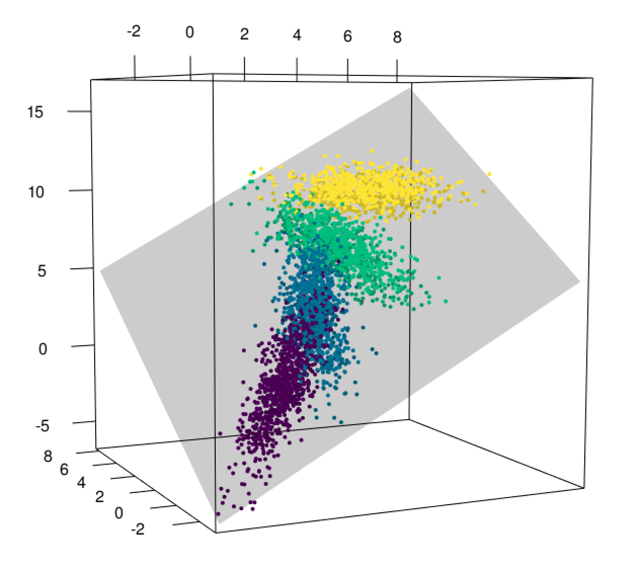
(a) Projection in $\mathbb{R}^{3}$

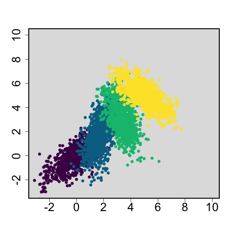
(b) $Y_{x}V$

(c) $Y_{x}V_{\perp}$

Figure 1: An illustration of high-dimensional data, $Y$, colored according to discretized levels of a covariate, $X$, and projected into low-dimension subspaces. Colors a) The projection of $Y$ into $\mathbb{R}^{3}$. In this example, the differences in both the means and covariances of $Y_{x}$ are confined to a two-dimensional envelope, $\mathcal{E}_{\mathcal{M}}(\mathcal{U})$ (grey plane), spanned by $V$. b) The data projected onto the $\mathcal{E}_{\mathcal{M}}(\mathcal{U})$, $Y_{x}V$, have means, $\phi_{x}$, and covariances $\Psi_{x}$ that co-vary with $x$. c) The orthogonal projection of the data, $Y_{x}V_{\perp}$ has equal means and covariances across all $x$.

Suppose that $Y$ is an $n\times p$ matrix of $n$ independent observations on $p$ correlated normally distributed features conditional on an $n\times q$ matrix of covariates, $X$. We use $y_{i}$ and $x_{i}$ to denote the $i$th row of $Y$ and $X$ respectively and allow both the the mean and covariance of $y_{i}$ to depend on $x_{i}$. Here, $y_{i}\sim N(\alpha_{0}+\mu_{x_{i}},\Sigma_{x_{i}})$ and thus the joint density of $Y$ given $X$ is given by

$$p(Y|X,\Sigma,n)\propto l(\Sigma_{x},\mu_{x}:Y,X)=\prod_{i}|\Sigma_{x_{i}}|^{-1/2}\operatorname{etr}\left(-\Sigma_{x}^{-1}(y_{i}-\alpha_{0}-\mu_{x_{i}})^{T}(y_{i}-\alpha_{0}-\mu_{x_{i}})/2\right)$$ (4)

where etr denotes the exponentiated trace. Following the strategies proposed in envelope and shared subspace models, we make the assumption that there exists a low-dimensional subspace which includes all of the variation in $Y$ that is associated with $X$. The projection of $Y$ onto the orthogonal subspace is invariant to $X$. We formalize this idea by making use of the following definition:

Definition 1.

Let $\mathcal{M}=\{\Sigma_{x_{i}}:i=1,\ldots,n\}$ be the collection of $p\times p$ symmetric positive definite matrices matrices associated with the residual covariance of each observation $i$, and let $\mathcal{U}=\text{span}(\mu_{x_{1}},\ldots,\mu_{x_{n}})$ be the span of the conditional means for each observation. We say that the $\mathcal{M}$-envelope of $\mathcal{U}$, $\mathcal{E}_{\mathcal{M}}({\mathcal{U}})$, is the intersection of all subspaces that contain $\mathcal{\mathcal{U}}$ and that reduce each member of $\mathcal{M}$.

This is closely related to the definition proposed in Su and Cook (2013), with the difference that we do not presuppose a linear mean model for $\mu_{x}$, and we further allow $\Sigma_{x}$ to differ for all observations. To instantiate this idea in a model, we posit that:

$$\mu_{x} =\phi_{x}V^{T}$$ (5)

$$\Sigma_{x} =V\Psi_{x}V^{T}+V_{\perp}\Psi_{0}V_{\perp}^{T}.$$

$V\in\mathcal{V}_{s,p}$, is an element of the Stiefel manifold, which consists of all $p\times s$ semi-orthogonal matrices and $V_{\perp}\in\mathcal{V}_{p-s,p}$ is a $p\times(p-s)$ semi-orthogonal matrix whose columns form the basis for the subspace of immaterial variation. If $s$ is the smallest dimension satisfying Equation 5, then the span of $V$ is the $\mathcal{M}$-envelope of $\mathcal{U}$, the smallest subspace of material variation. This is evident since $YV\sim N(\phi_{x},\Psi_{x}\otimes I_{n})$ depends on $x$, but $YV_{\perp}\sim N(0,\Psi_{0}\otimes I_{n})$ is invariant to changes in $X$ (see Figure 1). $\phi_{x}$ is the $s$-dimensional projected-data mean, $E[YV\mid X=x]$ and $\Psi_{x}$ is the $s\times s$ projected-data covariance matrix, $\rm{Cov}(YV\mid X=x)$. Throughout, we let model 5 be parameterized by $\theta$, where $\phi_{x}=f^{\mu}_{\theta}(x)$ is a function from $\mathbb{R}^{q}\to\mathbb{R}^{s}$ and $\Psi_{x}=f^{\Sigma}_{\theta}(x)$ a function from $\mathbb{R}^{q}\to\mathcal{S}^{+}_{s}$, the space of $s$-dimensional symmetric positive definite matrices.

Model 5 generalizes previously proposed response envelope models. In the classic response envelope model, $f^{\mu}_{\theta}(x)$ is linear in $x$, i.e. $\phi_{x}=x\eta$ and $f_{\theta}^{\Sigma}(x)$ is constant i.e. $\Psi_{x}=\Psi_{1}$ (Cook et al., 2010). Su and Cook (2013) extend the response envelope model to allow $\Psi_{x}$ to vary with a categorical predictor in the $p\ll n$ setting, i.e. $\Psi_{x}=\Psi_{k}$ if $x=k$, for $k\in\{1,\ldots,K\}$. Franks and Hoff (2019) also assume categorical covariates, but focus on the multi-group covariance estimation problem in the $p>n$ setting with $f^{\mu}_{\theta}(x)=0\leavevmode\nobreak\ \forall x$. Due to the high dimensionality of problems considered, they take $\Psi_{0}$ to be diagonal so that $\Sigma_{x}$ follows the spiked covariance model (Johnstone, 2001).

In many settings, more sophisticated assumptions about the structure of $\Psi_{x}$ are warranted. For example, if the groups are related, a hierarchical covariance model on $\Psi_{x}$ may be more appropriate (Bouriga and Féron, 2013; Hoff, 2009). We focus on the more general setting in which $\Psi_{x}$ varies with continuous covariates. Hoff and Niu (2012) propose a linear covariance regression model which specifies that the differences in $\Psi_{x_{i}}$ and $\Psi_{x_{j}}$ for any $i\neq j$ can be described by a rank $K$ matrix. Others have generalized this method for more flexible non-parametric models on $\Psi_{x}$ (Fox and Dunson, 2015).

In this work, we make use of both the spiked covariance assumption and the linear covariance regression model and posit that

$$\Sigma_{x} =V\Psi_{x}V^{T}+\sigma^{2}I$$ (6)

$$\Psi_{x} =\sum^{K}_{k}B_{k}xx^{T}B_{k}+A$$ (7)

where $x$ is a $q$-vector, $B_{k}$ is an $s\times q$ matrix and A is a $s\times s$ symmetric positive semi-definite matrix. The first equation corresponds to the spiked covariance assumption and the second equation is the linear covariance model proposed by Hoff and Niu (2012, 2019). Although the spiked model is unlikely to hold in practice, it is a particularly useful approximation in large $p$, small $n$ settings, where there is not enough power to accurately estimate more than a small number of factors of the covariance matrix (Gavish and Donoho, 2014). We assume the linear mean model $\phi_{x}=x\eta$ but this can also be generalized. To our knowledge, our approach is the first envelope model proposed for joint mean and covariance regression.

3 Inference

If a basis for the subspace of material variation, $V$, were known a priori, then we could estimate $\phi_{x}$ and $\Psi_{x}$ directly from the projected data $YV$. This would be much more efficient than estimating parameters from the full data $Y$, especially when $s$ is small relative to $p$. In practice, $V$ is not known, and thus must also be inferred. As such, a two-stage approach is commonly used, in which we first estimate the subspace of material variation, and then conditional on the inferred subspace, estimate $\phi_{x}$ and $\Psi_{x}$. $V$ is only identifiable up to rotations, since we can always reparameterize Equation 5 so that $\tilde{\phi}_{x}=\phi_{x}R$, $\tilde{\Psi}_{x}=R^{T}\Psi_{X}R$, and $\tilde{V}=VR$ for any $s\times s$ rotation matrix $R$. However, the projection matrix $VV^{T}\in\mathcal{G}_{p,s}$ is identifiable, where $\mathcal{G}_{p,s}$ is the Grassmannian manifold which consists of all $s$-dimensional subspaces of $\mathbb{R}^{p}$ (Chikuse, 2012). Although only the projection matrix $VV^{T}$ is identifiable, in practice most algorithms for subspace inference use what Cook et al. (2010) call a “coordinate-based” approach, by maximizing an objective function parameterized by a basis $V$ over the Stiefel manifold. Many efficient algorithms for coordinate-based envelope inference have been proposed (Cook and Zhang, 2015; Cook et al., 2016). Khare et al. (2017) propose an appealing method for joint Bayesian inference for all projected data parameters and the subspace in the response envelope model. However, Bayesian inference for semi-orthogonal matrices is challenging and their method does not scale for large $p$, e.g $p>50$.

In the context of their shared subspace covariance model, Franks and Hoff (2019) propose a hybrid empirical Bayes approach, in which they first infer $V$ using maximum marginal likelihood, and conditional on that subspace use Bayesian inference to infer the projected data covariance matrices. Building on this work, we propose a general strategy based on maximum marginal likelihood for $V$ by specifying prior distributions for the projected data parameters $\phi_{x}$ and $\Psi_{x}$:

$$[\hat{V},\hat{V}_{\perp}]=\underset{[V\leavevmode\nobreak\ V_{\perp}]\in\mathcal{V}_{p,p}}{\text{argmax}}\int_{\Theta}\mathcal{L}(V,V_{\perp},\theta;Y,X)p(\theta)d\theta$$

where $\mathcal{L}$ is the “complete data” likelihood and the integration is with respect to the appropriate measure (e.g. on the product space of $R^{s}$ and $\mathcal{S}^{+}$ for Example 1 below). Conditional on $\hat{V}$, an estimate of a basis for the material subspace of variation, we then conduct Bayesian inference for $\phi_{x}$ and $\Psi_{x}$ from the $s$-dimensional projected data by sampling from the posterior, $P(\phi,\Psi\mid Y\hat{V},X)$. The maximum marginal likelihood approach with conjugate prior distributions yields objective functions which are closely related to those used in previous work. Below we highlight some of these examples.

Example 1 (Response Envelopes, Cook et al. (2010)).

Assume the response envelope model (Equation 2). The response envelop model is a special case of model 5 with $\phi_{x}=X\eta$ with $\Psi_{x}=\Psi_{1}$ independent of $X$. Further, assume a priori that $\Psi_{i}\sim\text{inverse-Wishart}(U_{i},\nu_{i})$, $i\in\{0,1\}$ and that $\beta=\eta V$ has the multivariate matrix normal prior $\beta\mid(\Psi_{1},V)\sim MN(B_{0},V^{T}\Psi_{1}V\otimes\Lambda_{0})$. Then the marginal log-likelihood for $(V,V_{\perp})$, after integrating out $\theta=(\Psi_{1},\Psi_{0},\eta)$ is

$$\ell(V,V_{\perp})\propto-(n+s+\nu_{1}+1-q)/2\log|V^{T}(A+U_{1})V|-(n-(p-s)+\nu_{0}-1)/2\log|V_{\perp}^{T}(Y^{T}Y+U_{0})V_{\perp}|$$ (8)

where $A=(Y-XB_{n})^{T}(Y-XB_{n})+B_{n}^{T}\Lambda_{0}B_{n}$ and $B_{n}=(X^{T}X+\Lambda_{0})^{-1}X^{T}Y$.

Proof.

See appendix.

With the non-informative improper prior distributions $U_{i}=\mathbf{0}$ and $\Lambda_{0}=\mathbf{0}$ and $n\gg p$, this objective function is approximately proportional to the objective function originally proposed by Cook et al. (2010): $\ell(V,V_{\perp})=\log(|V^{T}AV|)+\log(V_{\perp}^{T}Y^{T}YV_{\perp})$ . In small $n$ settings, the difference in between these two objectives may be nontrivial. It should also be noted Equation 14 can be expressed as a function of $V$ only, since the subspace spanned by $V_{\perp}$ is identified by $V$ alone . The maximum marginal likelihood perspective also provides a principled way of including additional regularization by specifying appropriate prior parameters (see e.g. Yu and Zhu, 2010). Su et al. (2016) proposed an extension of to the envelope model to high-dimensional settings by a assuming a sparse envelope and modifying the usual envelope objective is augmented with a group lasso penalty on $V$. In our framework, such a penalty would equivalently be viewed as prior distribution over the space of semi-orthogonal matrices, $V$.

Example 2 (Shared Subspace Covariance Models, Franks and Hoff (2019)).

Assume the shared subspace model proposed by Franks and Hoff (2019), that is $\phi_{x}=0$ and $x$ is a single categorical predictor. Let $Y_{k}$ be the $n_{k}\times p$ matrix of observations for which $x$ has level $k$ and let $\Psi_{x}=\Psi_{k}$ denote the corresponding covariance matrix of $Y_{k}$. They assume a spiked covariance model, for which the data projected onto the subspace orthogonal to $V$ is isotropic, i.e. for which $\Psi_{0}=\sigma^{2}I$. $\Psi_{k}\sim inverse-Wishart(U_{k},\nu_{k})$ and $\sigma^{2}\sim\text{inverse-Gamma}(\alpha,\kappa)$. Then the marginal log-likelihood, after integrating out $\theta=(\Psi_{1},...\Psi_{k},\sigma^{2})$ is

$$\ell(V) \propto\sum_{k=1}^{K}\left[-(n_{k}/2-\nu_{1})/2\log|V^{T}(Y_{k}^{T}Y_{k}+U_{k})V|-(n_{k}(p-s)+\alpha)\log(\rm{tr}[(I-VV^{T})Y_{k}^{T}Y_{k}]/2+\kappa)\right]$$

Franks and Hoff (2019) propose a method for inferring the shared subspace using the EM algorithm, although the marginal distribution can be derived analytically, as above.

3.1 A Monte Carlo EM algorithm for Envelope Covariance Regression

In this Section we propose a general algorithm for inference in models satisfying Equation 5. We focus in particular on models for which $\Psi_{x}$ varies smoothly with continuous covariates although the algorithm can be applied more broadly. Following the strategy described in the previous section, a reasonable approach would be to specify a prior distribution for $\mu_{x}$ and $\Psi_{x}$ and analytically marginalize out these variables to determine an objective function for $V$. Unfortunately, for many covariance regression models, analytic marginalization is not possible. To address this challenge, we make use of the Expectation Maximization (EM) algorithm (Dempster et al., 1977). As a first step, we derive objective functions for $V$, a basis for the envelope assuming the projected data parameters, $\phi_{x}$ and $\Psi_{x}$ were known. The following results give us the relevant objective functions.

Theorem 1.

Assume a model satisfying Equation 5. Let the $\Psi_{0}\sim\text{inverse-Wishart}(U_{0},\nu_{0})$, and assume the $\Psi_{x_{i}}$ and mean $\phi_{x_{i}}$ are known. The marginal log-likelihood for $[V\leavevmode\nobreak\ V_{\perp}]$, integrating over, $\Psi_{0}$, with $\Psi_{x_{i}}$ and $\phi_{x_{i}}$ assumed known is:

$$\ell(V,V_{\perp};Y,X,\Psi_{x},\phi_{x}) =-\frac{1}{2}\sum_{i}\left[y_{i}V\Psi_{x_{i}}^{-1}V^{T}y_{i}^{T}-2\phi_{x_{i}}\Psi_{x_{i}}^{-1}V^{T}y_{i}^{T}\right]$$ (9)

$$\leavevmode\nobreak\ \leavevmode\nobreak\ \leavevmode\nobreak\ -\frac{(n+(p-s)+\nu_{0}+1)}{2}\log|V_{\perp}^{T}(Y^{T}Y+U_{0})V_{\perp}|$$

When $p$ is large, the above objective function may lead to high variance estimators, since $Y^{T}Y$ is a poor estimator of the marginaly covariance of $Y$ in the large $p$, small $n$ setting (Dempster, 1969; Stein, 1975). One option for high-dimensional inference is to enforce sparsity by penalizing the bases, $V$, with many non-zero rows. Another alternative, which is consistent with the above model is to use a strong informative prior for $\Psi_{0}$ by specifying a positive semidefinite matrix $U_{0}$ and an appropriately large value for $\nu_{0}$. A related approach for dealing with large $p$, small $n$ data, we make use of the spiked covariance model described in Section 2 , Equation 6. Our proposed objective function for the spiked model is given in the following corollary.

Corollary 1.

Assume a model satisfying Equation 6 and a prior for $\sigma^{2}\sim\text{inverse-Gamma}(\alpha,\kappa)$. The marginal log-likelihood for $V$, integrating over $\sigma^{2}$, assuming $\Psi_{x_{i}}$ and $\phi_{x_{i}}$ are known is:

$$\ell(V;Y,X,\Psi_{x},\phi_{x}) =-\frac{1}{2}\sum_{i}\left[y_{i}V\Psi_{x_{i}}^{-1}V^{T}y_{i}^{T}-2\phi_{x_{i}}\Psi_{x_{i}}^{-1}V^{T}y_{i}^{T}\right]$$ (10)

$$\leavevmode\nobreak\ \leavevmode\nobreak\ \leavevmode\nobreak\ -\left(\frac{(n(p-s)}{2}-\alpha\right)\log(\frac{1}{2}||Y||_{F}^{2}-\frac{1}{2}||YV||_{F}^{2}+\kappa)$$

Of course $\Psi_{x_{i}}$ and $\phi_{x_{i}}$ are not known in practice. As such, we use of the EM algorithm for $V$, under an appropriate prior for the model parameters for the projected data mean and covariance regression. Let $M^{(t)}_{x_{i}}=E[\phi_{x_{i}}\Psi^{-1}_{x_{i}}\mid V_{t},x_{i}]$ and $K^{(t)}_{x_{i}}=E[\Psi^{-1}_{x_{i}}\mid V_{t},x_{i}]$, where the expectation is taken with respect to $p(\theta\mid V_{t},Y,X)$. We then make use of Corollary 1, replacing projected data parameters with conditional posterior mean estimates for the M-step of the EM algorithm:

$$\ell(V,V_{\perp};M^{(t)}_{x},K^{(t)}_{x}) =-\frac{1}{2}\sum_{i}\left[y_{i}VK^{(t)}_{x_{i}}V^{T}y_{i}^{T}-2M^{(t)}_{x_{i}}V^{T}y_{i}^{T}\right]$$ (11)

$$\leavevmode\nobreak\ \leavevmode\nobreak\ \leavevmode\nobreak\ -\left(\frac{(n(p-s)}{2}-\alpha\right)\log(\frac{1}{2}||Y||_{F}^{2}-\frac{1}{2}||YV||_{F}^{2}+\kappa)$$

The steps involved in the MCEM approach are described Algorithm 1. Below, we provide more detail about the E- and M-steps.

Initialize $V_{0}\in\mathcal{V}_{p,s}$;

while $||V_{t}-V_{t-1}||_{F}>\epsilon$ do

       E-step:

       for $i\leftarrow 1$ to $n$ do

             $M^{(t)}_{x_{i}}\leftarrow E[\phi_{x_{i}}\Psi_{x_{i}}^{-1}\mid V_{t-1},Y]$;

             $K^{(t)}_{x_{i}}\leftarrow E[\Psi_{x_{i}}^{-1}\mid V_{t-1},Y]$;

            

       end for

      M-step:

        $[V_{t},V_{\perp t}]\leftarrow\underset{[V\leavevmode\nobreak\ V_{\perp}]\in\mathcal{V}_{p,s+r}}{\text{argmax }}\ell(V,V_{\perp};M^{(t)}_{x},K^{(t)}_{x})$, Equation 11;

      

end while

Algorithm 1 EM Subspace Estimation Algorithm

M-Step: As shown in Algorithm 1, the M-step of the EM algorithm requires optimizing an objective function over $\mathcal{V}_{p,s}$. Following existing work, we use the optimization method proposed by Wen and Yin (2013) and implemented in the the package rstiefel (Hoff and Franks, 2019) to find a basis for the subspace that minimizes the log-complete likelihood (Equation 11). This feasible search algorithm has complexity of order $O(ps^{2}+s^{3})$, and as such can be very fast when the dimension of the envelope is much smaller than $p$. This is usually assumed to be the case for large $p$, small $n$ problems, since we typically require that $s<n\ll p$. The matrix derivative, $\frac{d\ell}{dV}$ which is required for optimization is given in the Appendix.

(Monte Carlo) E-Step: The E-step involves computing $M^{(t)}_{x_{i}}=E[\phi_{x_{i}}\Psi_{x_{i}}^{-1}\mid V_{t-1},Y]$ and $K^{(t)}_{x_{i}}=E[\Psi_{x_{i}}^{-1}\mid V_{t-1},Y]$. However, for arbitrary models on $\phi_{x_{i}}$ and $\Psi_{x_{i}}$, the expectations $M^{(t)}_{x}$ and $K^{(t)}_{x}$ are also not analytically tractable. Here, we propose a Monte Carlo EM algorithm (MCEM) (Levine and Casella, 2001). We approximate $M^{(t)}_{x}$ and $K^{(t)}_{x}$ with MCMC samples at each iteration of Algorithm 1. Although MCMC is computationally expensive, for our motivating application we assume dimension of the envelope is small. As such, Bayesian inference for $\phi_{x_{i}}$ and $\Psi^{-1}_{x_{i}}$ can be approximated quickly. Importantly, any tractable Bayesian models for the inferring the posterior distribution $p(\phi_{x},\Psi_{x}\mid YV,X=x)$ can be used in this framework.

Many models are possible for $\phi_{x}$ and $\Psi_{x}$. In this work, we demonstrate the utility of our method for Bayesian covariance regression (Hoff, 2009; Fox and Dunson, 2015). We apply Monte Carlo EM algorithm with the the covariance regression model of Hoff and Niu (2012) for it’s simplicity, interpretability, and the availability of R package implementation covreg (Niu and Hoff, 2014). Although we focus on covariance regression in this work, our R code implements Algorithm 1 for any Bayesian model for $\phi_{x}$ and $\psi_{x}$ for, provided a user supplied function to compute appropriate posterior means (Franks, 2020).

3.2 Rank Selection and Initialization

Rank selection: A major challenge in any low rank method is choosing the appropriate rank. Several model selection criteria can be used to help facilitate this choice. Common approaches, including AIC, BIC, likelihood ratio tests and cross-validation, have all been applied in similar envelope models (Cook et al., 2010, 2013, 2016; Hoff and Niu, 2012). Following existing work, as a fast and useful heuristic, we propose applying asymptotically optimal (in mean squared error) singular value threshold for low rank matrix recovery with noisy data in the large $p$, small $n$ setting (Gavish and Donoho, 2014) and used a reducing covariance model by Franks and Hoff (2019). This rank estimation procedures is motivated under spiked covariance model and is a function of median singular value of the data matrix and the ratio of the features to the sample size, $p/n$. When all of the covariates are categorical, our approach is equivalent to the rank selection procedure in Franks and Hoff (2019). In Section 4 we explore the implications of misspecifying the envelope dimension.

Initialization: Since optimization over the Stiefel manifold is non-convex, choosing a good (i.e. $\sqrt{n}$-consistent) initial estimate of $V$ is important (Cook et al., 2016). Note that

$$\text{Cov}(Y) =\beta\text{Cov}(X)\beta^{T}+E[\Sigma_{X}]$$

$$=V\left(\eta\text{Cov}(X)\eta^{T}+E[\Psi_{x}]\right)V^{T}+V_{\perp}\Psi_{0}V_{\perp}^{T}$$

so that a subset of the right singular vectors of $Y$ consistently estimate $\mathcal{E}_{\mathcal{M}}(\beta)$. As such, one approach is to initialize $V$ to the first $s$ right singular vectors of $Y$. In our analyses, we take the first $q$-columns of $V$ to be a basis for of $\hat{\beta}_{\text{OLS}}$, of the OLS solution. For the remaining $s-q$ initial values of $V$, we choose the first $s-q$ right singular vectors of the residual $Y-X\hat{\beta}_{OLS}$. Cook and Zhang (2015) consider a sequential 1D algorithm, in which each column of $V$ is updated in a coordinate-wise fashion. They find that this fast way to initialization $V$ and could also be useful in our setting.

4 Simulation Studies

In the response envelope model, there can be drastic efficiency gains for the mean regression coefficients, in particular when the envelope has small dimension and $||\Psi_{0}||\gg||\Psi_{1}||$ (Cook et al., 2010). In this work, we explore the factors that improve efficiency of estimators for $\Psi_{x}$, focusing in this in this Section on the behavior and robustness of the proposed inferential approach in simulation. We use the following model throughout:

$$Y =X\mathbf{\eta}V+\epsilon_{x}$$ (12)

$$\Psi_{x} =\sum_{k}^{K=q}\Gamma_{k}x_{i}x_{i}^{T}\Gamma_{k}^{T}+\sigma^{2}I$$

$$\epsilon_{x} \sim N(0,V\Psi_{x}V^{T}+\sigma^{2}V_{\perp}V_{\perp}^{T})$$

where $X_{n\times q}\sim N(0,1)$, $\eta_{q\times s}\sim N(0,\tau^{2})$, $\Gamma_{s\times q}\sim N(0,1)$ are matrices with i.i.d random entries. We set $n=100$ and $s=4$ and evaluate covariance estimates using Stein’s loss, $L_{S}(\Psi_{x},\hat{\Psi}_{x})=\text{tr}(\Psi_{x}^{-1}\hat{\Psi}_{x})-\log|\Psi_{x}^{-1}\hat{\Psi}_{x}|-p$ (Dey et al., 1985). The Bayes estimator for Stein’s loss is the inverse of the posterior mean of the precision matrix, ${\text{E}}[\Psi_{x_{i}}^{-1}|Y,X,V]^{-1}$ which we estimate using MCEM (Section 3.1). In the simulations below, we compare the true covariance for observation $i$, $V^{T}\Sigma_{x_{i}}V=\Psi_{x_{i}}$ to the fitted values

$$\hat{\Psi}_{x} =V^{T}\hat{\Sigma}_{x_{i}}V$$ (13)

$$=(V^{T}\hat{V}){\text{E}}[\Psi_{x_{i}}^{-1}|Y,X,\hat{V}]^{-1}\hat{(}\hat{V}^{T}V)+\hat{\sigma}^{2}V^{T}\hat{V}_{\perp}\hat{V}_{\perp}^{T}V$$

Accurate estimates of $\Psi_{x}$ depend on the accuracy of both the subspace estimates, $\hat{V}$, as well as estimates of projected data covariance matrices $\hat{\Psi}_{x}$. In this Section we explore the robustness of our method to misspecification of chosen envelope dimension and also evaluate the effect that mean level differences have on inference for the covariance regression.

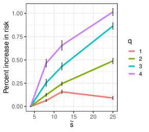
(a) Effect of specified envelope dimension

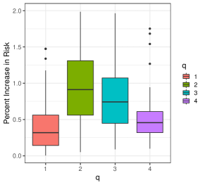
(b) Joint vs two-stage inference

Figure 2: a) Percentage increase in risk for covariance estimates due to misspecification of the subspace dimension relative to estimates using the true subspace dimension. We plot the mean percentage increase in loss as a function of the assumed subspace dimension, $\tilde{s}$ for data generated with $s=4$. Bars represent bootstrap 95% confidence intervals. b) Box plots of percentage increase in Stein’s loss for covariance estimates as a function of the number of covariates. When there are more covariates, mean-levels provide more information about the full subspace spanned by $V$. In this simulation, this gain is partially offset by the increase in covariance parameters as a function of $q$.

Misspecification of the Subspace Dimension: In practice, selecting the appropriate dimension, $s$, for the subspace of material variation is a challenging task. In this simulation, we evaluate the increase in loss when fitting model with assumed envelope dimension $\tilde{s}>s$. Envelope covariance regression with $\tilde{s}=p$ is equivalent to running covreg on the full $p$-dimensional data. Since inference in the covariance regression model is not computational tractable for large $\tilde{s}$, here we consider a relatively small-scale analysis: we generate data according to model proposed in Equation 12 where $s=4$ and where $p=25$ but fit the model assuming $\tilde{s}\in\{4,8,12,25\}$. We set $\tau=3$ and $\sigma^{2}=1$ and calculate the average Stein’s loss, $L_{\tilde{s}}=\frac{1}{n}\sum_{i}L_{\tilde{s}}(\Psi_{x_{i}},\hat{\Psi}_{x_{i}})$ on $M=100$ i.i.d. datasets. For each dataset, we fit our model at each value of $\tilde{s}$.

For the proposed data generating process, the distribution of Stein’s loss is heavily right skewed. In order to highlight the relative performance of the various estimators, we report the mean percentage increase in loss for all $\tilde{s}>s$, $\frac{1}{M}\sum_{m}^{M}\frac{L^{m}_{\tilde{s}}-L^{m}_{s}}{L^{m}{s}}$ relative to the loss for $\tilde{s}=s$, Figure 2(a). Although the true data generating model is nested in all models for which $\tilde{s}>s=4$, there can be substantial efficiency gains when the chosen dimension is close to the true low dimensional subspace. The efficiency gains are also generally larger for larger values of $q$, since the mean regression provides more information about the envelope.

Quantifying the Effect of the Mean Differences on Covariance Estimation: Here, we further investigate the effect of the mean on covariance matrix inference. We compare two approaches to inference: we consider a two stage approach in which we regress out the mean and then fit a covariance regression on the residual and compare this to the Monte Carlo EM algorithm for the envelope algorithm proposed in Section 3. The two-stage approach ignores the parametric link between the mean and residual covariance and thus a loss of efficiency is expected. We quantify the magnitude of this efficiency loss by again calculating Stein’s loss over $m=100$ i.i.d. datasets. We run experiments with $s=4,q\in\{1,2,3,4\}$ and $p=100$ and again plot percentage increase in Stein’s loss for the two-stage approach relative to the MCEM envelope approach, Figure 2(b). In general, $\text{rank}(\beta)\leq\text{rank}(V)=s$, with equality possible only if $q\geq s$. Our results show that efficient estimates of $\Psi_{x}$ are possible when $\text{rank}(\beta)\geq s$ and $||\beta||$ large, that is, when $\text{span}(V)$ can be identified precisely from mean levels differences alone. However, in the linear model, when $s\gg q$ the efficiency gains from incorporating information about mean differences may be more moderate. In this simulation we also assume that $\Psi_{x}$ varies by a rank $q$ matrix so these gains are partially offset by the fact that there $q^{2}s$ parameters to infer for the covariance regression (Equation 12).

5 Application to metabolomic data

In this Section we demonstrate the utility of the subspace covariance regression model in our motivating application, an analysis of hetereogeneity in metabolomic data. Metabolomics is the study of small molecules, known as metabolites, which include sugars, amino acids, and vitamins, amongst many others. These small molecules represent the products of interactions between genes, proteins and the environment, and make up the structural and functional building blocks of all organisms. As such, metabolomics can provide a detailed view into the physiological states of cells. By integrating measurements on the identities and abundances of these metabolites, we can develop a deeper understanding into the factors that shape phenotypic variation (Nicholson et al., 1999; Fiehn, 2002; Joyce and Palsson, 2006). Methods for analyzing metabolomic data stem from a long history of chemometrics, the field devoted to multivariate analysis of measurements on chemical systems (Wold, 1995). There are many tools for multivariate analysis of metabolomics including partial least squares methods, metabolite set enrichment analyses, and methods based on graphical models (Sun and Weckwerth, 2012; Xia et al., 2015). Interestingly, partial least squares methodology, which has its origin in chemometrics, is closely related to envelope methods (Cook et al., 2013).

Although many tools have been developed to analyze large multivariate metabolomic datasets, the vast majority of these methods focus on quantifying changes in mean metabolite levels across conditions. Quantifying metabolite co-dependence is a less studied problem, despite it’s importance. It is particularly relevant when there are unobserved factors which influence the relationship between covariates and the outcome. The effects of such unmeasured factors can manifest themselves as covariance heterogeneity. Specifically, we can view the covariance regression model proposed by Hoff and Niu (2012) as a linear interaction model with unobserved covariates: their covariance regression model can be equivalently expressed as the linear model $Y=\mu_{x_{i}}+\sum_{k}B_{k}x_{i}z_{ik}+\epsilon$ where $x_{i}$ is an observed covariate (e.g. age) and $z_{ik}\sim N(0,1)$ is an unobserved covariate (e.g. diet and lifestyle).

In this analysis, we demonstrate how estimates of covariance heterogeneity can improve our understanding of the biological mechanisms of aging. There have been many metabolomic studies on aging and age-related diseases (Jové et al., 2014; Kristal and Shurubor, 2005; Kristal et al., 2007), most of which have focused on changes in mean-levels of metabolite. However, even after accounting for variation in mean levels, significant heteoregeneity across chronological age groups remains (Lowsky et al., 2014), because unmeasured factors like diet, lifestyle and epigenetics are thought to have different effects on the metabolome at different ages (Horvath and Raj, 2018; Kristal et al., 2007; Brunet and Rando, 2017; Robinson et al., 2018).

Understanding how covariability amongst metabolites evolves with age is a largely unstudied problem, in part due to the challenges of modeling covariate-dependent covariance matrices. One notable exception is Le Goallec and Patel (2019), who look at how age influences co-dependency among 50 metabolic biomarkers in large population of individuals ($n=27508$). They compute all pairwise Pearson correlations between biomarkers at yearly age-bins and analyze trends in these correlations. They find that in general correlations tend to decrease with age. In this paper, we analyze the metabolomics of aging using our large $p$, small $n$ dataset using our envelope approach.

Here, we analyze metabolomic assays on cerebrospinal fluid data from 85 human subjects at ages ranging from 20 years old to 86 years old. The samples were assayed using both targeted and untargeted metabolite profiling LC-MS/MS experiments (Roberts et al., 2012; Dunn et al., 2013). The targeted data includes 108 known metabolites and their corresponding abundances (i.e. $p\approx n$). For the untargeted data we analyze approximately $2100$ metabolites which have measured abundances for at least 95% of the subjects (i.e. $p\gg n$). For missing value imputation in the untargeted data, we use Amelia, a software package for imputation in multivariate normal data (Honaker et al., 2011). In Figure 3 we depict exploratory plots which indicate that after OLS regression, pairwise correlations between residual metabolite abundances vary by age. These plots suggest covariance regression is warranted with this data.

(a) Residual metabolite correlations (increasing with age)

(b) Residual metabolite correlations (decreasing with age)

Figure 3: Residual Pearson correlations between metabolites show monotone trends after OLS regression. Observations are divided into five equal-sized groups, with age group 1 being the youngest individuals and age group 5 being the oldest individuals. Some metabolite pairs indicate increasing Pearson correlation with age whereas others indicate decreasing correlations with age.

As such, we fit the envelope covariance regression model (Equations 6 and 7) including both age and sex as covariates. We use the rank-estimation method proposed by Gavish and Donoho (2014) and discussed in Section 3.2. For the targeted analysis we infer that $s=18$ and for the untargeted analysis $s=17$.

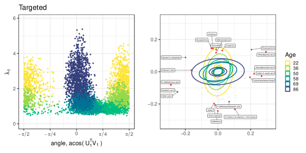
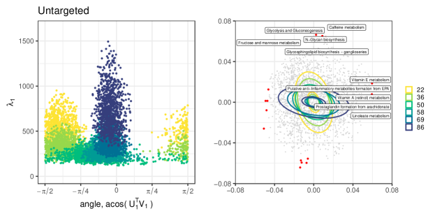
Figure 4: Posterior summaries for age-dependent covariance matrices on the targeted (top) and untargeted (bottom) dataset. Following Franks and Hoff (2019), we summarize the posterior distribution of the covariance matrices in terms of their eigenvalue and eigenvectors. Left) posterior samples of the largest eigenvalue and orientation of the first principal component on a two-dimensional subspace of $VV^{T}$ that describes the largest difference between the youngest and oldest male individuals. Right) A variant of the PCA biplot on the subspace of variation. Contours depict the posterior mean covariance matrices at different ages. Points reflect the metabolites with the largest factor loadings. For targeted data we include the names of metabolites with the largest factor loadings, whereas for the untargeted analysis, we include pathways enrichment analysis mummichog.

Following an approach proposed by Franks and Hoff (2019) we visualize posterior eigen-summaries on two dimensional subspaces of the envelope which are chosen to reflect the largest a posteriori significant differences between age groups. Since the specific basis $\hat{V}$ for the inferred envelope is arbitrary, we make a change of basis to one whose first components reflect larger differences between chosen groups of interest. For example, let $R$ denote the $s\times s$ orthogonal matrix of eigenvectors of the matrix $\hat{\Psi}_{\text{80,F}}-\hat{\Psi}_{\text{20,F}}$, the difference in projected ata covariance matrices for an 80 year old female and a 20 year old female. Then let $\tilde{V}=\hat{V}R$ be the rotated basis for the inferred envelope, ordered according to directions which maximize the difference in the projected data covariance matrices of old (i.e. 80 years old) and young (i.e. 20 years old) females. In Figure 4 we summarize inferred covariance matrices by plotting covariance summary statistics $\tilde{V}^{T}\Sigma_{x}\tilde{V}$, for male subjects at six different ages at roughly equal intervals and include results for female samples in the Appendix. In the left column of Figure 4 we plot posterior samples of $\Psi_{x}$ colored by age. Each point is a Monte Carlo sample of the largest eigenvalue $\lambda_{1}$ and the corresponding angle of the principal eigenvector, $U_{1}$, relative to the new coordinates defined by the first column of $\tilde{V}$. The right column depicts a variant of a PCA biplot, with the contours illustrating the posterior mean of $\tilde{V}\hat{\Psi}_{x}\tilde{V}^{T}$. The points indicate the feature loadings on two columns of $\tilde{V}$.

The top panels of Figure 4 depict results from the targeted analysis ($p=108$) and the bottom panel depicts results from the untargeted analysis ($p=2113$). In both of these figures, in older individuals there is higher variance among the metabolites with large loadings in the first component direction and lower variance for metabolites in the second direction. The opposite is true for young individuals. That the samples for the oldest and youngest individuals do not overlap suggests that these differences are significant a posteriori. For example, in the targeted analysis, we see that kynurenine and indole are anti-correlated along the second principal component direction, and have high variance in young individuals and lower variance in older individuals. A related metabolite, indole-3-acetic acid has higher variance in older individuals. These particular metabolites are associated with tryptophan metabolism, known to be one of the most important pathways associated with aging and age-related disease (Van der Goot and Nollen, 2013). Coefficients for these metabolites are also significant in the mean-regression (See Appendix).

For the untargeted data, metabolite identities are not known, only their mass-to-charge ratio and retention times. As such, we use the package mummichog for inferring significantly enriched metabolomic functional groups from high throughput, untargeted metabolomic data (Li et al., 2013). We use the absolute value of the loadings along each principle axis (the columns of $\tilde{V}$) as inputs to mummichog, since the values represent correlated features with high variability. Significantly enriched pathways associated with each principal axis are noted in the figure on the bottom right. For older individuals, we infer that there is higher variance in metabolites associated with pathways listed on the right (e.g. Vitamin A or E metabolism). In contrast, younger individuals seem to have more variable metabolite levels in pathways associated with the pathways listed on the top (e.g. Glycolysis and Gluconeogenesis or fructose and mannose metabolism). We also ran pathway enrichment on the mean coefficients for both age and sex (see Appendix). Some of the enriched pathways that were found to have metabolites with significant mean-level differences differ from those identified using the inferred covariance parameters. This suggests that additional insight can be gained by analyzing covariance heterogeneity that cannot be gleaned from mean level differences alone.

6 Discussion

In this paper, we extend the classic response envelope model to settings in which residual covariance matrices vary with continuous predictors. Unlike previous work, which primarily focuses on mean estimation in the linear model, we demonstrate that envelope models can also be used to improve inferences for covariance heterogeneity in the large $p$, small $n$ setting. Our work extends the hetereoskedastic envelope model (Su and Cook, 2013) and shared subspace of model of Franks and Hoff (2019) by accounting for continuously varying covariates. We demonstrate our approach using a linear Bayesian covariance regression model Hoff and Niu (2012); Niu and Hoff (2019), but our method is compatible with any Bayesian model for joint mean and covariance regression. We can also incorporate many of the extensions proposed in existing literature. For example, sparsifying penalities can be used as an alternative to the spiked model for high-dimensional inference Su et al. (2016) and can easily be integrated into the objective function. Although we assume normally distributed data, we can also extend the shared subspace approach to account for heavy tailed data, by modeling the outcome as a scale mixture of normal distributions (e.g. see Ding et al., 2019).

Finally, while we focus on linear mean and covariance models in this work, the Monte Carlo EM framework can be extended to non-linear and nonparametric models by leveraging other existing models for Bayesian inference in this setting. Tree-based models, like multivariate Bayesian Additive Regress Trees (BART) (Chipman et al., 2010) could be used as a non-parametric alternative for $\phi_{x}$. As noted, we have implemented the Monte Carlo EM algorithm as a practical tool for inference in many of these more elaborate envelope-based models (Franks, 2020).

Supporting Information for “Reducing Subspace Models for Large-Scale Covariance Regression” by Alexander Franks

Maximum Marginal Likelihood Derivations for Previously Proposed Models

Example 1 (Response Envelopes, Cook et al. (2010)).

Assume the response envelope model (Equation 2). The response envelop model is a special case of model 5 with $\phi_{x}=X\eta$ with $\Psi_{x}=\Psi_{1}$ independent of $x$. Further, assume a priori that $\Psi_{1}\sim\text{inverse-Wishart}(U_{1},\nu_{1})$, $\Psi_{0}\sim\text{inverse-Wishart}(U_{0},\nu_{0})$ and that $\eta$ has the multivariate matrix normal prior $\eta\mid(\Psi_{1},V)\sim MN(\eta_{0},\Psi_{1}\otimes\Lambda_{0})$. Then the marginal log-likelihood for $(V,V_{\perp})$, after integrating out $\theta=(\Psi_{1},\Psi_{0},\eta)$ is

$$\ell(V,V_{\perp})\propto-(n+s+\nu_{1}+1-q)/2\log|V^{T}(A+U_{1})V|-(n-(p-s)+\nu_{0}-1)/2\log|V_{\perp}^{T}(Y^{T}Y+U_{0})V_{\perp}|$$ (14)

where $A=(Y-XB_{n})^{T}(Y-XB_{n})+B_{n}^{T}\Lambda_{0}B_{n}$ and $B_{n}=(X^{T}X+\Lambda_{0})^{-1}X^{T}Y$.

Proof.

Let $Z=YV$, $\beta=\eta V^{T}$, and $V=[V,V_{\perp}]$ and $\Sigma=V\Psi_{1}V^{T}+V_{\perp}\Psi_{0}V^{T}_{\perp}$. The full likelihood can be written as:

$$p(Y\mid V,V_{\perp},\eta,\Psi_{0},\Psi_{1}) \propto|\Sigma|^{-n/2}\text{etr}(-1/2(Y-X\beta)\Sigma^{-1}(Y-X\beta)^{T})$$ (15)

$$\propto|V_{\perp}\Psi_{0}V_{\perp}^{T}+V\Psi_{1}V^{T}|^{-n/2}\text{etr}(-1/2(Y-X\beta)(V_{\perp}\Psi_{0}^{-1}V_{\perp}^{T}+V\Psi_{1}^{-1}V^{T})(Y-X\beta)^{T})$$ (16)

$$\propto|\Psi_{0}|^{-n/2}\text{etr}(-1/2V_{\perp}^{T}Y^{T}YV_{\perp}\Psi_{0}^{-1})|\Psi_{1}|^{-n/2}\text{etr}(-1/2\left[(Z-X\eta)(Z-X\eta)^{T}\right]\Psi_{1}^{-1})$$ (17)

Under the proposed prior distributions the we have

$$p(\Psi_{0},\Psi_{1},\eta,Y\mid,X,V,V_{\perp})\propto$$ (18)

$$|\Psi_{0}|^{-n/2}\text{etr}(-1/2\Psi_{1}^{-1}V_{\perp}^{T}Y^{T}YV_{\perp})\times|\Psi_{0}|^{-(\nu_{0}+(p-s)+1)/2}\text{etr}(\Psi_{0}^{-1}V_{\perp}^{T}U_{0}V_{\perp})\times$$ (19)

$$|\Psi_{1}|^{-n/2}\text{etr}(-1/2\left[(Z-XH_{n})^{T}(Z-XH_{n})+(H_{0}-H_{n})^{T}\Lambda_{0}(H_{0}-H_{n})+(\eta-H_{n})^{T}\Lambda_{n}(\eta-H_{n})\right]\Sigma_{1}^{-1})\times$$ (20)

$$|\Psi_{1}|^{-(\nu_{1}+s+1)/2}\text{etr}(\Psi_{1}^{-1}V^{T}U_{1}V)$$ (21)

where $H_{n}=\Lambda_{n}^{-1}X^{T}YV$ and $\Lambda_{n}=(X^{T}X+\Lambda_{0})$. We compute the marginal likelihood of $V$ and $V_{\perp}$ as

$$p(Y,\mid V,V_{\perp},X)\propto \int p(V,V_{\perp},\Psi_{0},\Psi_{1},\eta\mid Y,X)d\eta d\Psi_{1}d\Psi_{0}$$ (22)

First we isolate all terms in 18 involving $\eta$ and integrate

$$\int\text{etr}(\left[\eta-H_{n})^{T}\Lambda_{n}(\eta-H_{n})\right]\Sigma_{1}^{-1})d\eta\propto|\Psi_{1}|^{q/2}|$$

since the integrand is an unnnormalized multivariate normal density. Thus

$$p(Y,\Psi_{0},\Psi_{1},\mid V,V_{\perp},X)\propto |\Psi_{0}|^{-n/2}\text{etr}(-1/2V_{\perp}\Psi_{0}^{-1}V_{\perp}^{T}Y^{T}Y)\times$$ (23)

$$|\Psi_{1}|^{-(n-q)/2}\text{etr}(-1/2\left[(Z-XH_{n})^{T}(Z-XH_{n})+(H_{0}-H_{n})^{T}\Lambda_{0}(H_{0}-H_{n})\right]\Psi_{1}^{-1})\times$$ (24)

$$|\Psi_{0}|^{-(\nu_{0}+(p-s)+1)/2}\text{etr}(\Psi_{0}^{-1}V_{\perp}^{T}U_{0}V_{\perp})|\Psi_{1}|^{-(\nu_{1}+s+1)/2}\text{etr}(\Psi_{1}^{-1}V^{T}U_{1}V)$$ (25)

Next we isolate terms involving $\Psi_{1}$ and integrate:

$$\int|\Psi_{1}|^{-(n-q+\nu_{1})/2}\text{etr}(-1/2\left[(Z-XH_{n})^{T}(Z-XH_{n})+(H_{0}-H_{n})^{T}\Lambda_{0}(H_{0}-H_{n})+U_{1}\right]\Psi_{1}^{-1})d\Psi_{1}$$ (27)

which is proportional to an inverse-Wishart($(Z-XH_{n})^{T}(Z-XH_{n})+(H_{0}-H_{n})^{T}\Lambda_{0}(H_{0}-H_{n})+U_{1},(n-q+\nu_{1})$) density with normalizing constant proportional to

$$|(Z-XH_{n})^{T}(Z-XH_{n})+(H_{0}-H_{n})^{T}\Lambda_{0}(H_{0}-H_{n})+U_{1}|^{-(n-q+s+\nu_{1})/2}=$$ (28)

$$|V^{T}(Y-XB_{n})^{T}(Y-XB_{n})+(B_{0}-B_{n})^{T}\Lambda_{0}(B_{0}-B_{n})+U_{1})V|^{-(n-q+s+\nu_{1})/2}=$$ (29)

$$|V^{T}AV|^{-(n-q+s+\nu_{1})/2}$$ (30)

Finally we integrate out $\Sigma_{0}$,

$$=\int|\Sigma_{0}|^{-n/2}\text{etr}(-1/2(V_{\perp}^{T}Y^{T}YV_{\perp}+V_{\perp}^{T}U_{0}V_{\perp})\Sigma_{0}^{-1})d\Sigma_{0}$$ (31)

$$=|V_{\perp}^{T}(Y^{T}Y+U_{0})V_{\perp}|^{-\frac{(n+(p-s)+\nu_{0}+1)}{2}}$$ (32)

Combining equations 30 and 32 we have the marginal liklihood of $(V,V_{\perp})$:

$$p(Y\mid V,V_{\perp},X) \propto|VAV^{T}|^{-(n+s+\nu_{1}+1-q)/2}|V^{T}(Y^{T}Y+U_{0})V|^{-(n+s+\nu_{0}+1)/2}$$

$$A =(Y^{T}-B_{n}^{T})(Y-XB_{n})+B_{n}^{T}\Lambda_{0}B_{n}+U_{1}$$

$$B_{n} =(X^{T}X+\Lambda_{0})^{-1}X^{T}Y$$

With the non-informative improper prior distributions $U_{i}=\mathbf{0}$ and $\Lambda_{0}=\mathbf{0}$ and $n\gg p$, this objective function is approximately proportional to the objective function originally proposed by Cook et al. (2010): $\ell(V,V_{\perp})=\log(|V^{T}AV|)+\log(V_{\perp}^{T}Y^{T}YV_{\perp})$ . In small $n$ settings, the difference in between these two objectives may be nontrivial. It should also be noted Equation 14 can be expressed as a function of $V$ only, since the subspace spanned by $V_{\perp}$ is identified by $V$ alone . The maximum marginal likelihood perspective also provides a principled way of including additional regularization by specifying appropriate prior parameters (see e.g. Yu and Zhu, 2010). Su et al. (2016) proposed an extension of to the envelope model to high-dimensional settings by a assuming a sparse envelope and modifying the usual envelope objective is augmented with a group lasso penalty on $V$. In our framework, such a penalty would equivalently be viewed as prior distribution over the space of semi-orthogonal matrices, $V$.

Example 2 (Shared Subspace Covariance Models, Franks and Hoff (2019)).

Assume the shared subspace model proposed by Franks and Hoff (2019), that is $\phi_{x}=0$ and $x$ is a single categorical predictor. Let $Y_{k}$ be the $n_{k}\times p$ matrix of observations for which $x$ has level $k$ and let $\Psi_{x}=\Psi_{k}$ denote the corresponding covariance matrix of $Y_{k}$. They assume a spiked covariance model, for which the data projected onto the subspace orthogonal to $V$ is isotropic, i.e. for which $\Psi_{0}=\sigma^{2}I$. $\Psi_{k}\sim inverse-Wishart(U_{k},\nu_{k})$ and $\sigma^{2}\sim\text{inverse-Gamma}(\alpha,\kappa)$. Then the marginal log-likelihood, after integrating out $\theta=(\Psi_{1},...\Psi_{k},\sigma^{2})$ is

The complete likelihood can be expressed as:

$$\ell(V) \propto\sum_{k=1}^{K}\left[-(n_{k}-\nu_{1})/2\log|V^{T}(Y_{k}^{T}Y_{k}+U_{k})V|-(n_{k}(p-s)+\alpha)\log(\rm{tr}[(I-VV^{T})Y_{k}^{T}Y_{k}]/2+\kappa)\right]$$

Proof.

$$p(Y_{1},\ldots Y_{k}\mid V,V_{\perp}\sigma^{2}_{1}\ldots\sigma^{2}_{k},\Psi_{1}) \propto\prod|\Sigma_{k}|^{-n_{1}/2}\text{etr}(-1/2Y_{k}Y_{k}^{T}\Sigma_{k}^{-1})$$ (33)

$$\propto\prod|V\Psi_{k}V^{T}+\sigma^{2}_{k}(I-VV^{T})|^{-n_{1}/2}\text{etr}(-1/2Y_{k}Y_{k}^{T}(V\Psi_{k}V^{T}+\sigma^{2}_{k})^{-1})$$ (34)

$$\propto(\sigma_{k}^{2})^{-n_{1}(p-s)}\text{etr}(\frac{1}{\sigma_{k}^{2}}(I-VV^{T})Y_{k}^{T}Y_{k})|\Psi_{k}|^{-n_{1}/2}\text{etr}(-1/2Y_{k}Y_{k}^{T}V\Psi_{k}^{-1}V^{T})$$ (35)

We consider the marginal likelihood for an arbitrary group $k$, as each group is independent conditional on $V$. First, we integrate $\sigma_{k}^{2}$ given that $\sigma_{k}^{2}\sim\text{inverse-Gamma}(\alpha,\kappa)$:

$$p(Y_{k}\mid V,\Psi_{k}) \propto\int p(Y_{k}\mid V,\Psi_{k},\sigma_{k}^{2})p(\sigma_{2}k^{2})d\sigma_{k}^{2}$$ (36)

$$\propto\left(\int(\sigma_{k}^{2})^{-(p-s)}\text{etr}(\frac{1}{\sigma_{k}^{2}}(I-VV^{T})Y_{k}^{T}Y_{k})(\sigma^{2}_{k})^{\alpha-1}\text{etr}(\kappa/\sigma^{2}_{k})d\sigma_{k}^{2}\right)|\Psi_{k}|^{-n_{k}/2}\text{etr}(-1/2Y_{k}^{T}Y_{k}^{T}V\Psi_{k}^{-1}V^{T})$$ (37)

The integrand is a unnormalized inverse-Gamma($(n_{k}(p-s)+\alpha),\rm{tr}[(I-VV^{T})Y_{k}^{T}Y_{k}]/2+\kappa))$ density with normalizing constant proportional to $\rm{tr}[(I-VV^{T})Y_{k}^{T}Y_{k}]/2+\kappa)^{-(n_{k}(p-s)+\alpha)}$, so that

$$p(Y_{k}\mid V,\Psi_{k})\propto\rm{tr}[(I-VV^{T})Y_{k}^{T}Y_{k}]/2+\kappa)^{-(n_{1}p-s)+\alpha)}|\Psi_{k}|^{-n_{k}/2}\text{etr}(-1/2V^{T}Y_{k}^{T}Y_{k}^{T}V\Psi_{k}^{-1})$$ (38)

Next, we integrate out $\Psi_{k}$ given that $\Psi_{k}\sim\text{inverse-Wishart}(U_{k},\nu_{k})$.

$$p(Y_{k}\mid V) \propto\int p(Y_{k}\mid V,\Psi_{k})p(\Psi_{k}^{2})d\Psi_{k}$$ (39)

$$\propto\int\left(|\Psi_{k}|^{-n_{k}/2}\text{etr}(-1/2Y_{k}^{T}Y_{k}^{T}V\Psi_{k}^{-1}V^{T})|\Psi_{k}|^{-(\nu_{k}+s+1)/2}\text{etr}(-1/2U_{k}\Psi^{-1})d\Psi_{1}\right)$$ (40)

The integrand is a unnormalized inverse-Wishart($Y_{k}^{T}Y_{k}+U_{k},n_{k}+\nu_{1}))$ density with normalizing constant proportional to $|V^{T}(Y_{k}^{T}Y_{k}+U_{k})V|^{-(n_{k}/2-\nu_{k})/2}$ so that

$$p(Y_{k}\mid V) \propto|V^{T}(Y_{k}^{T}Y_{k}+U_{k})V|^{-(n_{k}-\nu_{k})/2}\rm{tr}[(I-VV^{T})Y_{k}^{T}Y_{k}]/2+\kappa)^{-(n_{k}(p-s)+\alpha)}$$ (41)

The objective function is then available as $\text{log}\prod_{k}p(Y_{k}\mid V)$ using the above result.

Franks and Hoff (2019) propose a method for inferring the shared subspace using the EM algorithm, although the marginal distribution can be derived analytically, as above.

Proof of Theorem 1

Theorem 1.

Assume a model satisfying Equation 5. Let the $\Psi_{0}\sim\text{inverse-Wishart}(U_{0},\nu_{0})$, and assume the $\Psi_{x_{i}}$ and mean $\phi_{x_{i}}$ are known. The marginal log-likelihood for $[V\leavevmode\nobreak\ V_{\perp}]$, integrating over, $\Psi_{0}$, with $\Psi_{x_{i}}$ and $\phi_{x_{i}}$ assumed known is:

$$\ell(V,V_{\perp};Y,X,\Psi_{x},\phi_{x}) =-\frac{1}{2}\sum_{i}\left[y_{i}V\Psi_{x_{i}}^{-1}V^{T}y_{i}^{T}-2\phi_{x_{i}}\Psi_{x_{i}}^{-1}V^{T}y_{i}^{T}\right]$$ (42)

$$\leavevmode\nobreak\ \leavevmode\nobreak\ \leavevmode\nobreak\ -\frac{(n+(p-s)+\nu_{0}+1)}{2}\log|V_{\perp}^{T}(Y^{T}Y+U_{0})V_{\perp}|$$

Proof.

$$p(Y\mid X,V,V_{\perp}\Psi_{x},\Psi_{0},\phi_{x}) \propto\prod_{i}|\Sigma_{x_{i}}|^{-1/2}\text{etr}(-1/2(y_{i}-\phi_{x_{i}}V)(y_{i}-\phi_{x_{i}}V)^{T}\Sigma_{x_{i}}^{-1})$$ (43)

$$\propto\prod_{i}|V\Psi_{x_{i}}V^{T}+V_{\perp}\Psi_{0}V_{\perp}^{T}|^{-1/2}\text{etr}(-1/2(Y_{i}-\phi_{x_{i}}V)(Y_{i}-\phi_{x_{i}}V)^{T}(V\Psi_{x_{i}}^{-1}V^{T}+V_{\perp}\Psi_{0}^{-1}V_{\perp}^{T}))$$ (44)

$$\propto\left(\prod_{i}|\Psi_{x_{i}}|^{-1/2}\text{etr}(-1/2(Y_{i}-\phi_{x_{i}}V)(Y_{i}-\phi_{x_{i}}V)^{T}V\Psi_{x_{i}}^{-1}V^{T})\right)$$ (45)

$$\times|\Psi_{0}|^{-n/2}\text{etr}(-1/2YY^{T}V_{\perp}\Psi_{0}^{-1}V_{\perp}^{T}))$$ (46)

$$\propto\left(\prod_{i}|V\Psi_{x_{i}}V^{T}|^{-1/2}\text{etr}(-1/2(Y_{i}^{T}Y_{i}V\Psi^{-1}_{x_{i}}-2\phi_{x_{i}}\Psi^{-1}_{x_{i}}V)\right)$$ (47)

$$\times|V_{\perp}\Psi_{0}V_{\perp}^{T}|^{-n/2}\text{etr}(-1/2YY^{T}V_{\perp}\Psi_{0}^{-1}V_{\perp}^{T}))$$ (48)

Under the inverse-Wishart prior we integrate out $\Psi_{0}$:

$$p(Y\mid X,V,V_{\perp}\Psi_{x},\phi_{x}) \propto\int p(Y\mid X,V,V_{\perp}\Psi_{x},\phi_{x})p(\Psi_{0})d\Psi_{0}$$ (49)

$$\propto\left(\prod_{i}|V\Psi_{x_{i}}V^{T}|^{-1/2}\text{etr}(-1/2(y_{i}y_{i}V\Psi^{-1}_{x_{i}}-2\phi_{x_{i}}\Psi^{-1}_{x_{i}}V)\right)$$ (50)

$$\times\int|V_{\perp}\Psi_{0}V_{\perp}^{T}|^{-n/2}\text{etr}(-1/2YY^{T}V_{\perp}\Psi_{0}^{-1}V_{\perp}^{T}))|V_{\perp}\Psi_{0}V_{\perp}^{T}|^{-(\nu_{0}-1)}\text{etr}(V_{\perp}\Psi_{0}^{-1}V_{\perp}^{T}U_{0})d\Psi_{0}$$ (51)

The integrand is a unnormalized inverse-Wishart($V_{\perp}(Y^{T}Y+U_{0})V_{\perp},n+\nu_{0}))$ density with normalizing constant which is proportional to $|V_{\perp}^{T}(Y^{T}Y+U_{0})V_{\perp}V|^{-(n-\nu_{0})/2}$ so that

$$p(Y\mid X,V,V_{\perp}\Psi_{x},\phi_{x}) \propto \propto\left(\prod_{i}|V\Psi_{x_{i}}V^{T}|^{-1/2}\text{etr}(-1/2(y_{i}^{T}y_{i}V\Psi^{-1}_{x_{i}}-2\phi_{x_{i}}\Psi^{-1}_{x_{i}}V)\right)|V_{\perp}^{T}(Y^{T}Y+U_{0})V_{\perp}|^{-(n+(p-s)+\nu_{0})/2}$$ (52)

Corollary 2.

Assume a model satisfying Equation 6 and a prior for $\sigma^{2}\sim\text{inverse-Gamma}(\alpha,\kappa)$. The marginal log-likelihood for $V$, integrating over $\sigma^{2}$, assuming $\Psi_{x_{i}}$ and $\phi_{x_{i}}$ are known is:

$$\ell(V;Y,X,\Psi_{x},\phi_{x}) =-\frac{1}{2}\sum_{i}\left[y_{i}V\Psi_{x_{i}}^{-1}V^{T}y_{i}^{T}-2\phi_{x_{i}}\Psi_{x_{i}}^{-1}V^{T}y_{i}^{T}\right]$$ (53)

$$\leavevmode\nobreak\ \leavevmode\nobreak\ \leavevmode\nobreak\ -\left(\frac{(n(p-s)}{2}-\alpha\right)\log(\frac{1}{2}||Y||_{F}^{2}-\frac{1}{2}||YV||_{F}^{2}+\kappa)$$

Proof.

$$p(Y\mid X,V,V_{\perp}\Psi_{x},\Psi_{0},\phi_{x}) \propto\prod_{i}|\Sigma_{x_{i}}|^{-1/2}\text{etr}(-1/2(Y_{i}-\phi_{x_{i}}V)(Y_{i}-\phi_{x_{i}}V)^{T}\Sigma_{x_{i}}^{-1})$$ (54)

$$\propto\prod_{i}|V\Psi_{x_{i}}V^{T}+\sigma^{2}(I-VV^{T})|^{-1/2}\text{etr}(-1/2(Y_{i}-\phi_{x_{i}}V)(Y_{i}-\phi_{x_{i}}V)^{T}(V\Psi_{x_{i}}^{-1}V^{T}+\frac{1}{\sigma^{2}}(I-VV^{T}))$$ (55)

$$\propto\prod_{i}|\Psi_{x_{i}}|^{-1/2}\text{etr}(-1/2(Y_{i}-\phi_{x_{i}}V)(Y_{i}-\phi_{x_{i}}V)^{T}V\Psi_{x_{i}}^{-1}V^{T})$$ (56)

$$\times(\sigma^{2})^{-n(p-s)/2}\text{etr}(-1/2YY^{T}(I-VV^{T})/\sigma^{2})$$ (57)

Under the inverse-Gamma prior, we can integrate out $\sigma^{2}$

$$p(Y\mid X,V,\Psi_{x},\phi_{x}) \propto\int p(Y\mid X,V,\Psi_{x},\phi_{x})p(\sigma^{2})d\Psi_{0}$$ (59)

$$\propto\prod_{i}|V\Psi_{x_{i}}V^{T}|^{-1/2}\text{etr}(-1/2(Y_{i}^{T}Y_{i}V\Psi^{-1}_{x_{i}}-2\phi_{x_{i}}\Psi^{-1}_{x_{i}}V)$$ (60)

$$\times\int(\sigma^{2})^{-n(p-s)/2}\text{etr}(-1/2YY^{T}(I-VV^{T})/\sigma^{2}))(\sigma^{2})^{-\alpha}e^{(\kappa/\sigma^{2})}d\sigma^{2}$$ (61)

The integrand is a unnormalized inverse-Gamma($,n(p-s)+\alpha)$ density with normalizing constant which is proportional to

$$|\text{tr}(-1/2YY^{T}(I-VV^{T}))+\kappa|^{-(n(p-s)/2+\alpha)}=(1/2||Y||_{F}^{2}-1/2||YV||_{F}^{2}+\kappa)^{-(n(p-s)/2+\alpha)}$$ (62)

so that

$$p(Y\mid X,V,V_{\perp}\Psi_{x},\phi_{x})\propto$$ (63)

$$\left(\prod_{i}|V\Psi_{x_{i}}V^{T}|^{-1/2}\text{etr}(-1/2(Y_{i}^{T}Y_{i}V\Psi^{-1}_{x_{i}}-2\phi_{x_{i}}\Psi^{-1}_{x_{i}}V)\right)(1/2||Y||_{F}^{2}-1/2||YV||_{F}^{2}+\kappa)^{-(n(p-s)/2+\alpha)}$$ (64)

Metabolomic Analysis of Mean-level Results

Metabolite	P-value	T-statistic	Q-value
HIAA	0.000	6.189341	0.0000000
Cystine	0.000	5.893680	0.0000000
Kynurenine	0.000	5.806419	0.0000000
4-Aminobutyric acid	0.000	-5.177550	0.0000000
Glycerol 3-phosphate	0.000	-4.444250	0.0000000
Adenosine	0.000	-4.345212	0.0000000
Uridine	0.000	-4.173488	0.0000000
Decanoylcarnitine	0.000	3.977997	0.0000000
Acetamide	0.000	-3.911912	0.0000000
Uracil	0.000	-3.441107	0.0000000
Aspartic acid	0.000	3.411236	0.0000000
Acetylglucosamine	0.000	3.390308	0.0000000
Xanthine	0.000	3.360388	0.0000000
Carnitine	0.000	3.220702	0.0000000
alpha-ketoisovaleric acid	0.000	-3.032598	0.0000000
Acetylglycine	0.000	2.880037	0.0000000
Glycylproline	0.002	3.288615	0.0127059
Glycine	0.006	2.790219	0.0360000
Levulinic acid	0.006	-2.746456	0.0341053
4-Methylvaleric acid	0.006	-2.647026	0.0324000
Adenosyl-L-homocysteine	0.008	2.960800	0.0411429
Indole-3-acetic acid	0.008	2.765461	0.0392727
Glycoursodeoxycholic acid	0.010	-2.618862	0.0469565
Glycohyodeoxycholic acid	0.010	-2.604362	0.0450000
Fructose	0.010	-2.465946	0.0432000
Indole	0.012	-2.564810	0.0498462

Table 1: Targeted data. Metabolites whose mean levels vary significantly with age.

Pathway	P-value
Vitamin B3 (nicotinate and nicotinamide) metabolism	0.0105033
Nitrogen metabolism	0.0119318
Phosphatidylinositol phosphate metabolism	0.0125200
Drug metabolism - cytochrome P450	0.0184018
Vitamin E metabolism	0.0275607
Glutamate metabolism	0.0275607

Table 2: Untargeted data. Pathways associated with metabolites whose mean levels vary with age.

Metabolite	P-value	T-statistic	Q-value
Stearic acid	0	-3.319559	0
N,N’-Dicyclohexylurea	0	2.770768	0

Table 3: Targeted data. Metabolites whose mean levels vary significantly with sex.

Select Covariance Regression Results - Sex

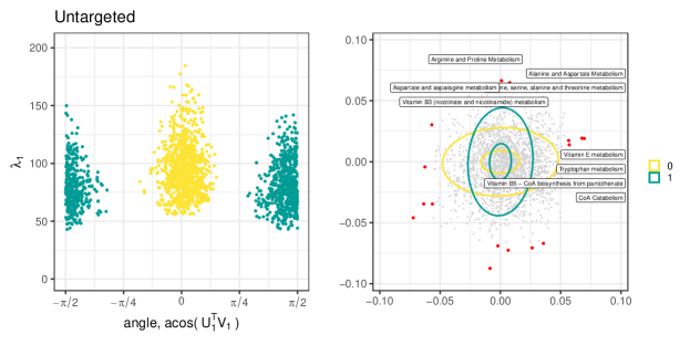
Figure 5: Posterior summaries for sex-dependent covariance matrices on the targeted (top) and untargeted (bottom) dataset. Following Franks and Hoff (2019), we summarize the posterior distribution of the covariance matrices in terms of their eigenvalue and eigenvectors. Left) posterior samples of the largest eigenvalue and orientation of the first principal component on a two-dimensional subspace of $VV^{T}$ that describes the largest difference between the youngest and oldest male individuals. Right) A variant of the PCA biplot on the subspace of variation. Contours depict the posterior mean covariance matrices at different ages. Points reflect the metabolites with the largest factor loadings. For targeted data we include the names of metabolites with the largest factor loadings, whereas for the untargeted analysis, we include pathways enrichment analysis mummichog.

References

- Boik (2002) Boik, R. J. (2002). Spectral models for covariance matrices. Biometrika 89(1), 159–182.
- Bouriga and Féron (2013) Bouriga, M. and O. Féron (2013). Estimation of covariance matrices based on hierarchical inverse-wishart priors. Journal of Statistical Planning and Inference 143(4), 795–808.
- Brunet and Rando (2017) Brunet, A. and T. A. Rando (2017). Interaction between epigenetic and metabolism in aging stem cells. Current opinion in cell biology 45, 1–7.
- Chandrasekaran et al. (2010) Chandrasekaran, V., P. A. Parrilo, and A. S. Willsky (2010). Latent variable graphical model selection via convex optimization. In 2010 48th Annual Allerton Conference on Communication, Control, and Computing (Allerton), pp. 1610–1613. IEEE.
- Chikuse (2012) Chikuse, Y. (2012). Statistics on special manifolds, Volume 174. Springer Science & Business Media.
- Chipman et al. (2010) Chipman, H. A., E. I. George, R. E. McCulloch, et al. (2010). Bart: Bayesian additive regression trees. The Annals of Applied Statistics 4(1), 266–298.
- Conway (1990) Conway, J. B. (1990). A course in functional analysis. 1990. Graduate Texts in Mathematics.
- Cook et al. (2013) Cook, R., I. Helland, and Z. Su (2013). Envelopes and partial least squares regression. Journal of the Royal Statistical Society: Series B (Statistical Methodology) 75(5), 851–877.
- Cook (2018) Cook, R. D. (2018). Principal components, sufficient dimension reduction, and envelopes.
- Cook and Forzani (2008) Cook, R. D. and L. Forzani (2008). Covariance reducing models: An alternative to spectral modelling of covariance matrices. Biometrika 95(4), 799–812.
- Cook et al. (2016) Cook, R. D., L. Forzani, and Z. Su (2016). A note on fast envelope estimation. Journal of Multivariate Analysis 150, 42–54.
- Cook et al. (2010) Cook, R. D., B. Li, and F. Chiaromonte (2010). Envelope models for parsimonious and efficient multivariate linear regression. Statistica Sinica, 927–960.
- Cook and Zhang (2015) Cook, R. D. and X. Zhang (2015). Algorithms for Envelope Estimation. Journal of Computational and Graphical Statistics 8600(March), 00–00.
- Danaher et al. (2014) Danaher, P., P. Wang, and D. M. Witten (2014). The joint graphical lasso for inverse covariance estimation across multiple classes. Journal of the Royal Statistical Society: Series B (Statistical Methodology) 76(2), 373–397.
- Dempster (1969) Dempster, A. P. (1969). Elements of continuous multivariate analysis. Technical report.
- Dempster et al. (1977) Dempster, A. P., N. M. Laird, and D. B. Rubin (1977). Maximum likelihood from incomplete data via the em algorithm. Journal of the Royal Statistical Society: Series B (Methodological) 39(1), 1–22.
- Dey et al. (1985) Dey, D. K., C. Srinivasan, et al. (1985). Estimation of a covariance matrix under stein’s loss. The Annals of Statistics 13(4), 1581–1591.
- Ding et al. (2019) Ding, S., Z. Su, G. Zhu, and L. Wang (2019). Envelope quantile regression. Statistica Sinica.
- Dunn et al. (2013) Dunn, W. B., A. Erban, R. J. Weber, D. J. Creek, M. Brown, R. Breitling, T. Hankemeier, R. Goodacre, S. Neumann, J. Kopka, et al. (2013). Mass appeal: metabolite identification in mass spectrometry-focused untargeted metabolomics. Metabolomics 9(1), 44–66.
- Fiehn (2002) Fiehn, O. (2002). Metabolomics—the link between genotypes and phenotypes. In Functional genomics, pp. 155–171. Springer.
- Flury (1987) Flury, B. (1987). Two generalizations of the common principal component model. Biometrika 74(1), 59–69.
- Fox and Dunson (2015) Fox, E. B. and D. B. Dunson (2015). Bayesian nonparametric covariance regression. The Journal of Machine Learning Research 16(1), 2501–2542.
- Franks (2020) Franks, A. M. (2020). enveloper. https://github.com/afranks86/envelopeR.
- Franks and Hoff (2019) Franks, A. M. and P. Hoff (2019). Shared subspace models for multi-group covariance estimation. Journal of Machine Learning Research 20(171), 1–37.
- Friedman et al. (2008) Friedman, J., T. Hastie, and R. Tibshirani (2008). Sparse inverse covariance estimation with the graphical lasso. Biostatistics 9(3), 432–441.
- Gavish and Donoho (2014) Gavish, M. and D. L. Donoho (2014). The optimal hard threshold for singular values is . Information Theory, IEEE Transactions on 60(8), 5040–5053.
- Heimberg et al. (2016) Heimberg, G., R. Bhatnagar, H. El-Samad, and M. Thomson (2016). Low dimensionality in gene expression data enables the accurate extraction of transcriptional programs from shallow sequencing. Cell Systems 2(4), 239–250.
- Hoff and Franks (2019) Hoff, P. and A. Franks (2019). rstiefel: Random Orthonormal Matrix Generation and Optimization on the Stiefel Manifold. R package version 1.0.0.
- Hoff (2009) Hoff, P. D. (2009). A hierarchical eigenmodel for pooled covariance estimation. Journal of the Royal Statistical Society: Series B (Statistical Methodology) 71(5), 971–992.
- Hoff and Niu (2012) Hoff, P. D. and X. Niu (2012). A covariance regression model. Statistica Sinica 22, 729–753.
- Honaker et al. (2011) Honaker, J., G. King, and M. Blackwell (2011). Amelia II: A program for missing data. Journal of Statistical Software 45(7), 1–47.
- Horvath and Raj (2018) Horvath, S. and K. Raj (2018). Dna methylation-based biomarkers and the epigenetic clock theory of ageing. Nature Reviews Genetics 19(6), 371.
- Johnstone (2001) Johnstone, I. M. (2001). On the distribution of the largest eigenvalue in principal components analysis. Annals of statistics, 295–327.
- Jové et al. (2014) Jové, M., M. Portero-Otín, A. Naudí, I. Ferrer, and R. Pamplona (2014). Metabolomics of human brain aging and age-related neurodegenerative diseases. Journal of Neuropathology & Experimental Neurology 73(7), 640–657.
- Joyce and Palsson (2006) Joyce, A. R. and B. Ø. Palsson (2006). The model organism as a system: integrating’omics’ data sets. Nature reviews Molecular cell biology 7(3), 198–210.
- Khare et al. (2017) Khare, K., S. Pal, Z. Su, et al. (2017). A bayesian approach for envelope models. The Annals of Statistics 45(1), 196–222.
- Kristal and Shurubor (2005) Kristal, B. S. and Y. I. Shurubor (2005). Metabolomics: opening another window into aging. Science of aging knowledge environment: SAGE KE 2005(26), pe19–pe19.
- Kristal et al. (2007) Kristal, B. S., Y. I. Shurubor, R. Kaddurah-Daouk, and W. R. Matson (2007). Metabolomics in the study of aging and caloric restriction. In Biological Aging, pp. 393–409. Springer.
- Le Goallec and Patel (2019) Le Goallec, A. and C. J. Patel (2019). Age-dependent co-dependency structure of biomarkers in the general population of the united states. Aging (Albany NY) 11(5), 1404.
- Lee and Su (2019) Lee, M. and Z. Su (2019). A review of envelope models.
- Levine and Casella (2001) Levine, R. A. and G. Casella (2001). Implementations of the monte carlo em algorithm. Journal of Computational and Graphical Statistics 10(3), 422–439.
- Li et al. (2013) Li, S., Y. Park, S. Duraisingham, F. H. Strobel, N. Khan, Q. A. Soltow, D. P. Jones, and B. Pulendran (2013). Predicting network activity from high throughput metabolomics. PLoS computational biology 9(7).
- Liland (2011) Liland, K. H. (2011). Multivariate methods in metabolomics–from pre-processing to dimension reduction and statistical analysis. TrAC Trends in Analytical Chemistry 30(6), 827–841.
- Lowsky et al. (2014) Lowsky, D. J., S. J. Olshansky, J. Bhattacharya, and D. P. Goldman (2014). Heterogeneity in healthy aging. Journals of Gerontology Series A: Biomedical Sciences and Medical Sciences 69(6), 640–649.
- Mardia et al. (1980) Mardia, K. V., J. T. Kent, and J. M. Bibby (1980). Multivariate analysis. Academic press.
- Meinshausen and Bühlmann (2006) Meinshausen, N. and P. Bühlmann (2006). High-dimensional graphs and variable selection with the lasso. The annals of statistics, 1436–1462.
- Nicholson et al. (1999) Nicholson, J. K., J. C. Lindon, and E. Holmes (1999). ’metabonomics’: understanding the metabolic responses of living systems to pathophysiological stimuli via multivariate statistical analysis of biological nmr spectroscopic data. Xenobiotica 29(11), 1181–1189.
- Niu and Hoff (2014) Niu, X. and P. Hoff (2014). covreg: A simultaneous regression model for the mean and covariance. R package version 1.0.
- Niu and Hoff (2019) Niu, X. and P. D. Hoff (2019). Joint mean and covariance modeling of multiple health outcome measures. The annals of applied statistics 13(1), 321.
- Roberts et al. (2012) Roberts, L. D., A. L. Souza, R. E. Gerszten, and C. B. Clish (2012). Targeted metabolomics. Current protocols in molecular biology 98(1), 30–2.
- Robinson et al. (2018) Robinson, O. J., M. C. Hyam, I. Karaman, R. C. Pinto, G. Fiorito, H. Gao, A. Heard, M.-R. Jarvelin, M. Lewis, R. Pazoki, et al. (2018). Determinants of accelerated metabolomic and epigenetic ageing in a uk cohort. bioRxiv, 411603.
- Schott (1991) Schott, J. R. (1991). Some tests for common principal component subspaces in several groups. Biometrika 78(4), 771–777.
- Stein (1975) Stein, C. (1975). Estimation of a covariance matrix. Rietz Lecture.
- Su and Cook (2013) Su, Z. and R. D. Cook (2013). Estimation of multivariate means with heteroscedastic errors using envelope models. Statistica Sinica 23(1), 213–230.
- Su et al. (2016) Su, Z., G. Zhu, X. Chen, and Y. Yang (2016). Sparse envelope model: efficient estimation and response variable selection in multivariate linear regression. Biometrika 103(3), 579–593.
- Sun and Weckwerth (2012) Sun, X. and W. Weckwerth (2012). Covain: a toolbox for uni-and multivariate statistics, time-series and correlation network analysis and inverse estimation of the differential jacobian from metabolomics covariance data. Metabolomics 8(1), 81–93.
- Van der Goot and Nollen (2013) Van der Goot, A. T. and E. A. Nollen (2013). Tryptophan metabolism: entering the field of aging and age-related pathologies. Trends in molecular medicine 19(6), 336–344.
- Wang et al. (2019) Wang, W., X. Zhang, and L. Li (2019). Common reducing subspace model and network alternation analysis. Biometrics 75(4), 1109–1120.
- Wen and Yin (2013) Wen, Z. and W. Yin (2013). A feasible method for optimization with orthogonality constraints. Mathematical Programming 142(1-2), 397–434.
- Wold (1995) Wold, S. (1995). Chemometrics; what do we mean with it, and what do we want from it? Chemometrics and Intelligent Laboratory Systems 30(1), 109–115.
- Xia et al. (2015) Xia, J., I. V. Sinelnikov, B. Han, and D. S. Wishart (2015). Metaboanalyst 3.0—making metabolomics more meaningful. Nucleic acids research 43(W1), W251–W257.
- Yu and Zhu (2010) Yu, Z. and L. Zhu (2010). Comments on” envelope models for parsimonious and efficient multivariate linear regression” by cook, d. and li, b. and chiaromonte. Statistica Sinica 20(3), 988.