A stochastic algorithm for fault inverse problems in elastic half space with proof of convergence

Darko Volkov Department of Mathematical Sciences, Worcester Polytechnic Institute, Worcester, MA 01609.
Abstract

A general stochastic algorithm for solving mixed linear and nonlinear problems was introduced in [11]. We show in this paper how it can be used to solve the fault inverse problem, where a planar fault in elastic half-space and a slip on that fault have to be reconstructed from noisy surface displacement measurements. With the parameter giving the plane containing the fault denoted by mm{\itbf m} and the regularization parameter for the linear part of the inverse problem denoted by C𝐶C, both modeled as random variables, we derive a formula for the posterior marginal of mm{\itbf m}. Modeling C𝐶C as a random variable allows to sweep through a wide range of possible values which was shown to be superior to selecting a fixed value [11]. We prove that this posterior marginal of mm{\itbf m} is convergent as the number of measurement points and the dimension of the space for discretizing slips increase. Simply put, our proof only assumes that the regularized discrete error functional for processing measurements relates to an order 1 quadrature rule and that the union of the finite-dimensional spaces for discretizing slips is dense. Our proof relies on trace class operator theory to show that an adequate sequence of determinants is uniformly bounded. We also explain how our proof can be extended to a whole class of inverse problems, as long as some basic requirements are met. Finally, we show numerical simulations that illustrate the numerical convergence of our algorithm.

Keywords: Linear and nonlinear inverse problems, Regularization, Convergence of random variables, Trace class operators.


1 Introduction

In [11], we introduced a numerical method for mixed linear and nonlinear inverse problems. This method applies to cases where the data for the inverse problem is corrupted by noise and where for each value of the nonlinear parameter, the underlying linear problem is ill-posed. Accordingly, regularizing this linear part is required. The norm used for the regularization process has to be multiplied by a scaling parameter, also called regularization parameter, denoted by C𝐶C throughout this paper. In [11], a Bayesian approach was adopted, and C𝐶C was modeled as a random variable. It was shown in [11] that this approach is superior to selecting C𝐶C using some standard method for linear inverse problems, such as the discrepancy principle, or the generalized cross validation. Loosely speaking, this can be explained by observing that for different values of the nonlinear parameter mm{\itbf m}, these classical methods will favor different values of C𝐶C, and as a result different values of the nonlinear parameter mm{\itbf m} cannot be fairly compared. Attempting to select a unique value of C𝐶C for all values of mm{\itbf m} leads to somehow better results, but as demonstrated in the last section of this paper, doing so pales in comparison to the method advocated in [11].
In this paper, we first derive in section 3 a specific version of the Bayesian posterior distribution of mm{\itbf m} following the method introduced in [11]. This version applies to an inverse problem in half space for the linear elasticity equations. In the direct problem, a slip field on an open surface that we will call a fault, gives rise to a displacement field. In the inverse problem, this field is measured on the plane on top of the half space at M𝑀M points. The linear part of the inverse problem consists of reconstructing the slip field on the fault. The nonlinear part consists of finding the geometry and the location of the fault. This formulation is commonly used in geophysics to model slow slip events in the vicinity of subduction zones, or the total displacement resulting from a dynamic earthquake, see [13, 14] and references therein. In this paper, the geometry of the fault is assumed to be planar, thus we choose the nonlinear parameter mm{\itbf m} to be in 3superscript3\mathbb{R}^{3}. The stochastic model considered in this paper is different from a model studied in an earlier paper by the same author [12]. As explained in section 3, the difference is that we here assume the regularization parameter C𝐶C for the linear part of the inverse problem to be a random variable and the covariance σ𝜎\sigma of the measurements is unknown. In section 3, the likelihood of σ𝜎\sigma is optimized based on the data and as a consequence the resulting posterior distribution function of mm{\itbf m} is entirely different from the simpler one used in [12]. Computing this new posterior is more intricate since it involves the random variable (m,C)m𝐶({\itbf m},C) instead of just mm{\itbf m} in [12]. The benefit of using this new posterior is that it leads to much better numerical results if the covariance σ𝜎\sigma of the measurements is unknown as shown in sections 6.2 and 6.3.
In section 4, we provide a mathematical proof of the soundness of our Bayesian approach for computing the posterior probability density of mm{\itbf m}. More precisely, we show that as the number of measurement points M𝑀M tends to infinity and the dimension of the space for discretizing slip fields tends to infinity, the probability of mm{\itbf m} to be further than a fixed η>0𝜂0\eta>0 from the true value m~~m\tilde{{\itbf m}} converges to zero if the noise level is low enough. Interestingly, although the derivation of the probability law of the posterior of mm{\itbf m} assumes that the noise is Gaussian, once this law is set the proof of convergence does not require the noise to be Gaussian. The proof assumes that the regularized discrete error functional for sampling measurements relates to an order 1 quadrature rule for C1superscript𝐶1C^{1} functions (which is verified by most commonly used quadrature rules) and that the union of the finite-dimensional spaces for discretizing slips is dense, a natural requirement that can be easily satisfied by combining adequate finite element spaces. The more difficult step in this proof of convergence requires showing that a sequence of determinants is uniformly bounded: this can be achieved by using trace class operator theory [6].
In section 5, for the reader’s convenience, we extend the formulation of our recovery method to more general inverse problems. We write down the expression of the posterior probability distribution that is at the core of our reconstruction method. A companion parallel sampling algorithm is given in [11], section 3.2. At the end of section 5 of this paper, we state a convergence theorem for the posterior probability distribution which is valid in this more general framework.
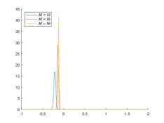
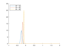
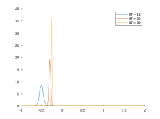
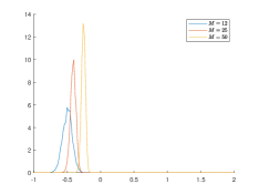
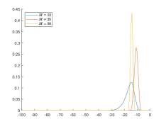
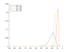
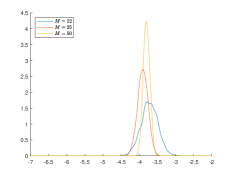
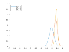
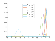
In section 6, we present numerical simulations that use our posterior probability distribution for reconstructing the geometry parameter mm{\itbf m}. The posterior marginals of mm{\itbf m} and of the regularization parameter C𝐶C are computed using the method of choice sampling due to the size of the search space. We used a modified version of the Metropolis algorithm which is well suited to parallel computing, [3]. This modified version was described in details in previous work, [11]. The computed posterior marginals shown in section 6 illustrate the theoretical convergence result proved in section 4: in the low noise case, as well as in the high noise case, the posterior marginals of mm{\itbf m} tighten around the true value m~~m\tilde{{\itbf m}} as the number of measurement points and the dimension of the space for discretizing slips increase, as expected from Theorem 4.1. Of course in the low noise case, the tightening is more narrow, also as expected from Theorem 4.1. In a final section, we show how using a simplistic method where different values of the regularization parameter C𝐶C are first fixed and then marginal posteriors of mm{\itbf m} are computed, leads to results that are impossible to interpret since there is no objective way to select an optimal C𝐶C for mixed linear and nonlinear problems if the variance of the noise is unknown.

2 Governing equations, inverse problem, and error functionals

2.1 Formulation of the direct and the inverse fault problems

Using standard rectangular coordinates, let x=(x1,x2,x3)xsubscript𝑥1subscript𝑥2subscript𝑥3{\itbf x}=(x_{1},x_{2},x_{3}) denote elements of 3superscript3\mathbb{R}^{3}. We define 3superscriptlimit-from3\mathbb{R}^{3-} to be the open half space x3<0subscript𝑥30x_{3}<0. The direct problem relies on the equations of linear elasticity with Lamé constants λ𝜆\lambda and μ𝜇\mu such that λ>0𝜆0\lambda>0 and λ+μ>0𝜆𝜇0\lambda+\mu>0. For a vector field 𝒱=(𝒱1,𝒱2,𝒱3)𝒱subscript𝒱1subscript𝒱2subscript𝒱3{\cal V}=({\cal V}_{1},{\cal V}_{2},{\cal V}_{3}), the stress vector in the direction e3esuperscript3{\itbf e}\in\mathbb{R}^{3} will be denoted by

Te𝒱=j=13(λdiv 𝒱δij+μ(i𝒱j+j𝒱i))ej.subscript𝑇e𝒱superscriptsubscript𝑗13𝜆div 𝒱subscript𝛿𝑖𝑗𝜇subscript𝑖subscript𝒱𝑗subscript𝑗subscript𝒱𝑖subscript𝑒𝑗\displaystyle T_{\itbf e}{\cal V}=\sum_{j=1}^{3}\left(\lambda\,\mbox{div }{\cal V}\,\delta_{ij}+\mu\,(\partial_{i}{\cal V}_{j}+\partial_{j}{\cal V}_{i})\right)e_{j}.

Let ΓΓ\Gamma be a Lipschitz open surface strictly included in 3superscriptlimit-from3\mathbb{R}^{3-} with normal vector nn{\itbf n} defined almost everywhere. We define the jump [𝒱]delimited-[]𝒱\mbox{$[$}{\cal V}\mbox{$]$} of the vector field 𝒱𝒱{\cal V} across ΓΓ\Gamma to be

[𝒱](x)=limh0+𝒱(x+hn)𝒱(xhn),delimited-[]𝒱xsubscriptsuperscript0𝒱xn𝒱xn\mbox{$[$}{\cal V}\mbox{$]$}({\itbf x})=\lim_{h\rightarrow 0^{+}}{\cal V}({\itbf x}+h{\itbf n})-{\cal V}({\itbf x}-h{\itbf n}),

for xx{\itbf x} in ΓΓ\Gamma, if this limit exists. Let 𝒰𝒰{\cal U} be the displacement field solving

μΔ𝒰+(λ+μ)div 𝒰=0 in 3Γ,𝜇Δ𝒰𝜆𝜇div 𝒰0 in superscriptlimit-from3Γ\displaystyle\mu\Delta{\cal U}+(\lambda+\mu)\nabla\mbox{div }{\cal U}=0\mbox{ in }\mathbb{R}^{3-}\setminus\Gamma, (2.1)
Te3𝒰=0 on the surface x3=0,subscript𝑇subscripte3𝒰0 on the surface subscript𝑥30\displaystyle T_{{\itbf e}_{3}}{\cal U}=0\mbox{ on the surface }x_{3}=0, (2.2)
Tn𝒰 is continuous across Γ,subscript𝑇n𝒰 is continuous across Γ\displaystyle T_{{\itbf n}}{\cal U}\mbox{ is continuous across }\Gamma, (2.3)
[𝒰]=𝒢 is a given jump across Γ,delimited-[]𝒰𝒢 is a given jump across Γ\displaystyle\mbox{$[$}{\cal U}\mbox{$]$}={\cal G}\mbox{ is a given jump across }\Gamma, (2.4)
𝒰(x)=O(1|x|2),𝒰(x)=O(1|x|3), uniformly as |x|,formulae-sequence𝒰x𝑂1superscriptx2formulae-sequence𝒰x𝑂1superscriptx3 uniformly as x\displaystyle{\cal U}({\itbf x})=O(\frac{1}{|{\itbf x}|^{2}}),\nabla{\cal U}({\itbf x})=O(\frac{1}{|{\itbf x}|^{3}}),\mbox{ uniformly as }|{\itbf x}|\rightarrow\infty, (2.5)

where e3subscripte3{\itbf e}_{3} is the vector (0,0,1)001(0,0,1). Let H~12(Γ)2superscript~𝐻12superscriptΓ2\widetilde{H}^{\frac{1}{2}}(\Gamma)^{2} be the space of restrictions to ΓΓ\Gamma of tangential fields in H12(D)2superscript𝐻12superscript𝐷2H^{\frac{1}{2}}(\partial D)^{2} supported in Γ¯¯Γ\overline{\Gamma}, where D𝐷D is a bounded domain in 3superscriptlimit-from3\mathbb{R}^{3-} such that ΓDΓ𝐷\Gamma\subset\partial D. In [13], we defined the functional space 𝐒𝐒{\bf S} of vector fields 𝒱𝒱{\cal V} defined in 3Γ¯superscriptlimit-from3¯Γ\mathbb{R}^{3-}\setminus{\overline{\Gamma}} such that 𝒱𝒱\nabla{\cal V} and 𝒱(1+r2)12𝒱superscript1superscript𝑟212\displaystyle\frac{{\cal V}}{(1+r^{2})^{\frac{1}{2}}} are in L2(3Γ¯)3superscript𝐿2superscriptsuperscriptlimit-from3¯Γ3L^{2}(\mathbb{R}^{3-}\setminus{\overline{\Gamma}})^{3} and we proved the following result.

Theorem 2.1

Let 𝒢𝒢{\cal G} be in H~12(Γ)2superscript~𝐻12superscriptΓ2\widetilde{H}^{\frac{1}{2}}(\Gamma)^{2}. The problem (2.1-2.4) has a unique solution in 𝐒𝐒{\bf S}. In addition, the solution 𝒰𝒰{\cal U} satisfies the decay conditions (2.5).

The following theorem shown in [13] asserts that 𝒢𝒢{\cal G} and ΓΓ\Gamma are uniquely determined from the data 𝒰𝒰{\cal U} given on a relatively open set of the plane x3=0subscript𝑥30x_{3}=0 if we know that ΓΓ\Gamma is planar.

Theorem 2.2

Let Γ1subscriptΓ1\Gamma_{1} and Γ2subscriptΓ2\Gamma_{2} be two planar open surfaces. For i𝑖i in {1,2}12\{1,2\}, assume that 𝒰isuperscript𝒰𝑖{\cal U}^{i} solves (2.1-2.5) for ΓisubscriptΓ𝑖\Gamma_{i} in place of ΓΓ\Gamma and 𝒢isuperscript𝒢𝑖{\cal G}^{i}, a tangential field in H~12(Γi)2superscript~𝐻12superscriptsubscriptΓ𝑖2\tilde{H}^{\frac{1}{2}}(\Gamma_{i})^{2}, in place of 𝒢𝒢{\cal G}. Assume that 𝒢isuperscript𝒢𝑖{\cal G}^{i} has full support in ΓisubscriptΓ𝑖\Gamma_{i}, that is, supp 𝒢i=Γi¯supp subscript𝒢𝑖¯subscriptΓ𝑖\mbox{supp }{\cal G}_{i}=\overline{\Gamma_{i}}. Let V𝑉V be a non empty open subset in {x3=0}subscript𝑥30\{x_{3}=0\}. If 𝒰1superscript𝒰1{\cal U}^{1} and 𝒰2superscript𝒰2{\cal U}^{2} are equal in V𝑉V, then Γ1=Γ2subscriptΓ1subscriptΓ2\Gamma_{1}=\Gamma_{2} and 𝒢1=𝒢2superscript𝒢1superscript𝒢2{\cal G}^{1}={\cal G}^{2}.

Theorems 2.1 and 2.2 were proved in [13] for media with constant Lamé coefficients and in [2] for more general Lamé systems. Similar results were obtained in [1] for layered media, albeit in a bounded domain.
The solution 𝒰𝒰{\cal U} to problem (2.1-2.4) can be expressed as the convolution on ΓΓ\Gamma

𝒰(x)=ΓH(x,y,n)𝒢(y)𝑑s(y),𝒰xsubscriptΓHxyn𝒢ydifferential-d𝑠y\displaystyle{\cal U}({\itbf x})=\int_{\Gamma}{\itbf H}({\itbf x},{\itbf y},{\itbf n}){\cal G}({\itbf y})\,ds({\itbf y}), (2.6)

where HH{\itbf H} is the Green tensor associated to the system (2.1-2.5), and nn{\itbf n} is the vector normal to ΓΓ\Gamma. The practical determination of this half space Green tensor HH{\itbf H} was studied in [9] and later, more rigorously, in [10]. Due to formula (2.6) we can define a continuous mapping from tangential fields 𝒢𝒢{\cal G} in H01(Γ)2subscriptsuperscript𝐻10superscriptΓ2H^{1}_{0}(\Gamma)^{2} to surface displacement fields 𝒰(x1,x2,0)𝒰subscript𝑥1subscript𝑥20{\cal U}(x_{1},x_{2},0) in L2(V)3superscript𝐿2superscript𝑉3L^{2}(V)^{3} where 𝒰𝒰{\cal U} and 𝒢𝒢{\cal G} are related by (2.1-2.5). This mapping is compact since H(x,y,n)Hxyn{\itbf H}({\itbf x},{\itbf y},{\itbf n}) is smooth for (x,y)xy({\itbf x},{\itbf y}) in V¯×Γ¯¯𝑉¯Γ\overline{V}\times\overline{\Gamma}. Theorem 2.2 asserts that this compact mapping is injective, so its inverse can be defined. As the inverse of a compact mapping is unbounded, finding 𝒢𝒢{\cal G} from 𝒰(x1,x2,0)𝒰subscript𝑥1subscript𝑥20{\cal U}(x_{1},x_{2},0) has to involve regularization.

2.2 A regularized functional for the reconstruction of planar faults

Let R𝑅R be a bounded, non-empty, open set of the plane x3=0subscript𝑥30x_{3}=0. Let B𝐵B be a compact set of (a,b,d)𝑎𝑏𝑑(a,b,d) in 3superscript3\mathbb{R}^{3} such that

{(x1,x2,ax1+bx2+d):(x1,x2)R}conditional-setsubscript𝑥1subscript𝑥2𝑎subscript𝑥1𝑏subscript𝑥2𝑑subscript𝑥1subscript𝑥2𝑅\displaystyle\{(x_{1},x_{2},ax_{1}+bx_{2}+d):(x_{1},x_{2})\in R\}

is included in the half-space x3<0subscript𝑥30x_{3}<0. We introduce the notations

m=(a,b,d),m𝑎𝑏𝑑\displaystyle{\itbf m}=(a,b,d),
Γm={(x1,x2,ax1+bx2+d):(x1,x2)R}.subscriptΓmconditional-setsubscript𝑥1subscript𝑥2𝑎subscript𝑥1𝑏subscript𝑥2𝑑subscript𝑥1subscript𝑥2𝑅\displaystyle\Gamma_{\itbf m}=\{(x_{1},x_{2},ax_{1}+bx_{2}+d):(x_{1},x_{2})\in R\}.

It follows that the distance between ΓmsubscriptΓm\Gamma_{{\itbf m}} and the plane x3=0subscript𝑥30x_{3}=0 is bounded below by the same positive constant for all mm{\itbf m} in B𝐵B. We assume that slips 𝒢𝒢{\cal G} are supported in such sets ΓmsubscriptΓm\Gamma_{{\itbf m}}. We can then map all these fields into the rectangle R𝑅R. We thus obtain displacement vectors for xx{\itbf x} in V𝑉V by the integral formula

𝒰(x,𝒢,m)=RHm(x,y1,y2)𝒢(y1,y2)s𝑑y1𝑑y2,𝒰x𝒢msubscript𝑅subscriptHmxsubscript𝑦1subscript𝑦2𝒢subscript𝑦1subscript𝑦2𝑠differential-dsubscript𝑦1differential-dsubscript𝑦2\displaystyle{\cal U}({\itbf x},{\cal G},{\itbf m})=\int_{R}{\itbf H}_{\itbf m}({\itbf x},y_{1},y_{2}){\cal G}(y_{1},y_{2})sdy_{1}dy_{2}, (2.7)

for any 𝒢𝒢{\cal G} in H01(R)2subscriptsuperscript𝐻10superscript𝑅2H^{1}_{0}(R)^{2} and mm{\itbf m} in B𝐵B, where s𝑠s is the surface element on ΓmsubscriptΓm\Gamma_{\itbf m} and Hm(x,y1,y2)subscriptHmxsubscript𝑦1subscript𝑦2{\itbf H}_{\itbf m}({\itbf x},y_{1},y_{2}) is derived from the Green’s tensor HH{\itbf H} for yy{\itbf y} on ΓmsubscriptΓm\Gamma_{\itbf m}. We now assume that V𝑉V is a bounded open subset of the plane x3=0subscript𝑥30x_{3}=0. For a fixed 𝒰~~𝒰\tilde{{\cal U}} be in L2(V)superscript𝐿2𝑉L^{2}(V), and a fixed mm{\itbf m} in B𝐵B we define the regularized error functional

m,C(𝒢)=V|𝒰(x,𝒢,m)𝒰~(x))|2dx+CR|𝒢|2,\displaystyle{\cal F}_{{\itbf m},C}({\cal G})=\int_{V}|{\cal U}({\itbf x},{\cal G},{\itbf m})-\tilde{{\cal U}}({\itbf x}))|^{2}d{\itbf x}+C\int_{R}|\nabla{\cal G}|^{2}, (2.8)

where C>0𝐶0C>0 is the regularization parameter and 𝒢𝒢{\cal G} is in H01(R)2subscriptsuperscript𝐻10superscript𝑅2H^{1}_{0}(R)^{2}. Define the operator

𝒜msubscript𝒜m\displaystyle{\cal A}_{{\itbf m}} ::\displaystyle: H01(R)2L2(V)3subscriptsuperscript𝐻10superscript𝑅2superscript𝐿2superscript𝑉3\displaystyle H^{1}_{0}(R)^{2}\rightarrow L^{2}(V)^{3} (2.9)
𝒢RHm(x,y1,y2)𝒢(y1,y2)s𝑑y1𝑑y2.𝒢subscript𝑅subscriptHmxsubscript𝑦1subscript𝑦2𝒢subscript𝑦1subscript𝑦2𝑠differential-dsubscript𝑦1differential-dsubscript𝑦2\displaystyle{\cal G}\rightarrow\int_{R}{\itbf H}_{\itbf m}({\itbf x},y_{1},y_{2}){\cal G}(y_{1},y_{2})sdy_{1}dy_{2}.

It is clear that 𝒜msubscript𝒜m{\cal A}_{{\itbf m}} is linear, continuous, and compact. The functional m,Csubscriptm𝐶{\cal F}_{{\itbf m},C} can also be written as,

m,C(𝒢)=𝒜m𝒢𝒰~L2(V)32+C𝒢H01(R)22,subscriptm𝐶𝒢subscriptsuperscriptnormsubscript𝒜m𝒢~𝒰2superscript𝐿2superscript𝑉3𝐶subscriptsuperscriptnorm𝒢2subscriptsuperscript𝐻10superscript𝑅2\displaystyle{\cal F}_{{\itbf m},C}({\cal G})=\|{\cal A}_{{\itbf m}}{\cal G}-\tilde{{\cal U}}\|^{2}_{L^{2}(V)^{3}}+C\|{\cal G}\|^{2}_{H^{1}_{0}(R)^{2}}, (2.10)

where in H01(R)2subscriptsuperscript𝐻10superscript𝑅2H^{1}_{0}(R)^{2} we use the norm

𝒢H01(R)2=(R|𝒢|2)12.subscriptnorm𝒢subscriptsuperscript𝐻10superscript𝑅2superscriptsubscript𝑅superscript𝒢212\displaystyle\|{\cal G}\|_{H^{1}_{0}(R)^{2}}=(\int_{R}|\nabla{\cal G}|^{2})^{\frac{1}{2}}. (2.11)

In the remainder of this paper, for the sake of simplifying notations, both L2(V)3\|\,\|_{L^{2}(V)^{3}} and H01(R)2\|\,\|_{H^{1}_{0}(R)^{2}} will be abbreviated by \|\,\|; context will eliminate any risk of confusion.

Proposition 2.1

For any fixed mm{\itbf m} in B𝐵B and C>0𝐶0C>0, m,Csubscriptm𝐶{\cal F}_{{\itbf m},C} achieves a unique minimum m,Csubscriptm𝐶{\cal H}_{{\itbf m},C} in H01(R)2subscriptsuperscript𝐻10superscript𝑅2H^{1}_{0}(R)^{2}.

Proof: This result holds thanks to classic Tikhonov regularization theory (for example, see [8], Theorem 16.4). \Box

For m,Csubscriptm𝐶{\cal H}_{{\itbf m},C} as in the statement of Proposition 2.1 we set,

fC(m)=m,C(m,C).subscript𝑓𝐶msubscriptm𝐶subscriptm𝐶\displaystyle f_{C}({\itbf m})={\cal F}_{{\itbf m},C}({\cal H}_{{\itbf m},C}). (2.12)
Proposition 2.2

fCsubscript𝑓𝐶f_{C} is a Lipschitz continuous function on B𝐵B. It achieves its minimum value on B𝐵B.

Proof: This was proved in [12], Proposition 3.2. \Box
It is helpful to state a direct consequence of uniqueness Theorem 2.2 in terms of the operators 𝒜msubscript𝒜m{\cal A}_{\itbf m}.

Proposition 2.3

Let m,mmsuperscriptm{\itbf m},{\itbf m}^{\prime} be in B𝐵B and 𝒢,𝒢𝒢superscript𝒢{\cal G},{\cal G}^{\prime} be in H01(R)2subscriptsuperscript𝐻10superscript𝑅2H^{1}_{0}(R)^{2}. Assume that 𝒢𝒢{\cal G} or 𝒢superscript𝒢{\cal G}^{\prime} is non-zero. If 𝒜m𝒢=𝒜m𝒢subscript𝒜m𝒢subscript𝒜superscriptmsuperscript𝒢{\cal A}_{{\itbf m}}{\cal G}={\cal A}_{{\itbf m}^{\prime}}{\cal G}^{\prime} then m=mmsuperscriptm{\itbf m}={\itbf m}^{\prime} and 𝒢=𝒢𝒢superscript𝒢{\cal G}={\cal G}^{\prime}.

In the remainder of this paper, we only consider one-directional fields 𝒢𝒢{\cal G}. Accordingly, 𝒢𝒢{\cal G} can be considered to be a scalar function in the space H01(R)subscriptsuperscript𝐻10𝑅H^{1}_{0}(R), and 𝒜msubscript𝒜m{\cal A}_{\itbf m} becomes a linear operator from H01(R)subscriptsuperscript𝐻10𝑅H^{1}_{0}(R) to L2(V)3superscript𝐿2superscript𝑉3L^{2}(V)^{3}.

2.3 A functional for the reconstruction of planar faults from surface measurements at M𝑀M points

For j=1,..,Mj=1,..,M, let Pjsubscript𝑃𝑗P_{j} be points in V𝑉V, so on the surface x3=0subscript𝑥30x_{3}=0, and u~(Pj)~usubscript𝑃𝑗\tilde{{\itbf u}}(P_{j}) be measured displacements at these points. Let H𝐻H be a finite-dimensional subspaces of H01(R)superscriptsubscript𝐻01𝑅H_{0}^{1}(R). For 𝒢𝒢{\cal G} in H𝐻H and mm{\itbf m} in B𝐵B, define the functional

Fm,C(𝒢)=j=1MC(j)|(𝒜m𝒢u~)(Pj)|2+CR|𝒢|2,subscript𝐹m𝐶𝒢superscriptsubscript𝑗1𝑀superscript𝐶𝑗superscriptsubscript𝒜m𝒢~usubscript𝑃𝑗2𝐶subscript𝑅superscript𝒢2\displaystyle F_{{\itbf m},C}({\cal G})=\sum_{j=1}^{M}C^{\prime}(j)|({\cal A}_{{\itbf m}}{\cal G}-\tilde{{\itbf u}})(P_{j})|^{2}+C\int_{R}|\nabla{\cal G}|^{2}, (2.13)

where 𝒜msubscript𝒜m{\cal A}_{{\itbf m}} was defined in (2.9), and C>0𝐶0C>0 is the regularization parameter. We assume that the constants C(j)superscript𝐶𝑗C^{\prime}(j) are positive.

Proposition 2.4

The functional Fm,Csubscript𝐹m𝐶F_{{\itbf m},C} achieves a unique minimum on H𝐻H.

Proof: This results again from Tikhonov regularization theory. \Box
As Fm,Csubscript𝐹m𝐶F_{{\itbf m},C} achieves its minimum at some hm,Csubscripthm𝐶{\itbf h}_{{\itbf m},C} in H𝐻H,we set

fCdisc(m)=Fm,C(hm,C).subscriptsuperscript𝑓𝑑𝑖𝑠𝑐𝐶msubscript𝐹m𝐶subscripthm𝐶\displaystyle f^{disc}_{C}({\itbf m})=F_{{\itbf m},C}({\itbf h}_{{\itbf m},C}). (2.14)

The superscript ”disc” stands for discrete.

Proposition 2.5

fCdiscsubscriptsuperscript𝑓𝑑𝑖𝑠𝑐𝐶f^{disc}_{C} is a Lipschitz continuous function on B𝐵B and achieves its minimum value on B𝐵B.

Proof: The proof is similar to that of Proposition 2.2. \Box

3 Bayesian model derivation

We assume in our stochastic model that the geometry parameter m=(a,b,d)m𝑎𝑏𝑑{\itbf m}=(a,b,d) is in B𝐵B and the measurements u~(Pj)~usubscript𝑃𝑗\tilde{{\itbf u}}(P_{j}) are related by the equation

(u~(P1),,u~(PM))=δ+(𝒜mg(P1),,𝒜mg(PM))+,~usubscript𝑃1~usubscript𝑃𝑀𝛿subscript𝒜mgsubscript𝑃1subscript𝒜mgsubscript𝑃𝑀\displaystyle(\tilde{{\itbf u}}(P_{1}),...,\tilde{{\itbf u}}(P_{M}))=\delta+({\cal A}_{\itbf m}{\itbf g}(P_{1}),...,{\cal A}_{\itbf m}{\itbf g}(P_{M}))+{\cal E}, (3.1)

where 𝒜msubscript𝒜m{\cal A}_{\itbf m} is as in (2.9), gg{\itbf g} is in H𝐻H, and {\cal E} in 3Msuperscript3𝑀\mathbb{R}^{3M} is additive noise, which is modeled to be a random variable. The error term δ𝛿\delta is given by

(𝒜m(IΠ)(𝒢)(P1),,𝒜m(IΠ)(𝒢)(PM)),subscript𝒜m𝐼Π𝒢subscript𝑃1subscript𝒜m𝐼Π𝒢subscript𝑃𝑀\displaystyle({\cal A}_{\itbf m}(I-\Pi)({\cal G})(P_{1}),...,{\cal A}_{\itbf m}(I-\Pi)({\cal G})(P_{M})), (3.2)

where ΠΠ\Pi is the orthogonal projection from H01(R)subscriptsuperscript𝐻10𝑅H^{1}_{0}(R) to H𝐻H and 𝒢𝒢{\cal G} is in H01(R)subscriptsuperscript𝐻10𝑅H^{1}_{0}(R). δ𝛿\delta represents the part of the slip that cannot be reached by the finite dimensional model and g=Π𝒢gΠ𝒢{\itbf g}=\Pi{\cal G}. We assume in this section that {\cal E} follows a normal probability distribution with mean zero and diagonal covariance matrix σ2Isuperscript𝜎2𝐼\sigma^{2}I after rescaling by Csuperscript𝐶C^{\prime}, so altogether the diagonal of this covariance matrix is the vector in 3Msuperscript3𝑀\mathbb{R}^{3M} is

σ2(C(1)1,C(1)1,C(1)1,,C(M)1,C(M)1,C(M)1).superscript𝜎2superscript𝐶superscript11superscript𝐶superscript11superscript𝐶superscript11superscript𝐶superscript𝑀1superscript𝐶superscript𝑀1superscript𝐶superscript𝑀1\displaystyle\sigma^{2}(C^{\prime}(1)^{-1},C^{\prime}(1)^{-1},C^{\prime}(1)^{-1},...,C^{\prime}(M)^{-1},C^{\prime}(M)^{-1},C^{\prime}(M)^{-1}).

The 3M3𝑀3M dimensional vector (u~(P1),,u~(PM))~usubscript𝑃1~usubscript𝑃𝑀(\tilde{{\itbf u}}(P_{1}),...,\tilde{{\itbf u}}(P_{M})) will be denoted by u~~u\tilde{{\itbf u}}. Given our assumption on the noise {\cal E}, for a fixed mm{\itbf m} and gg{\itbf g} the random variable (𝒜mg(P1),,𝒜mg(PM))+subscript𝒜mgsubscript𝑃1subscript𝒜mgsubscript𝑃𝑀({\cal A}_{\itbf m}{\itbf g}(P_{1}),...,{\cal A}_{\itbf m}{\itbf g}(P_{M}))+{\cal E} is normal with mean (𝒜mg(P1),,𝒜mg(PM))subscript𝒜mgsubscript𝑃1subscript𝒜mgsubscript𝑃𝑀({\cal A}_{\itbf m}{\itbf g}(P_{1}),...,{\cal A}_{\itbf m}{\itbf g}(P_{M})) and covariance σ2Isuperscript𝜎2𝐼\sigma^{2}I. Accordingly, by (3.1), the probability density of u~δ~u𝛿\tilde{{\itbf u}}-\delta knowing the geometry parameter mm{\itbf m}, the slip field gg{\itbf g} and the variance σ𝜎\sigma is

ρ(u~δ|m,g,σ)exp(12σ2j=1MC(j)|𝒜mgu~|2(Pj)).proportional-to𝜌~uconditional𝛿mg𝜎12superscript𝜎2superscriptsubscript𝑗1𝑀superscript𝐶𝑗superscriptsubscript𝒜mg~u2subscript𝑃𝑗\displaystyle\rho(\tilde{{\itbf u}}-\delta|{\itbf m},{\itbf g},\sigma)\propto\exp(-\frac{1}{2\sigma^{2}}\sum_{j=1}^{M}C^{\prime}(j)|{\cal A}_{\itbf m}{\itbf g}-\tilde{{\itbf u}}|^{2}(P_{j})). (3.3)

Next, we assume that mm{\itbf m} in B𝐵B and gg{\itbf g} in H𝐻H are independent random variables. The prior distribution of mm{\itbf m}, ρprsubscript𝜌𝑝𝑟\rho_{pr}, is assumed to be uninformative, that is, ρpr(m)1B(m)proportional-tosubscript𝜌𝑝𝑟msubscript1𝐵m\rho_{pr}({\itbf m})\propto 1_{B}({\itbf m}). For the prior distribution of gg{\itbf g} knowing C𝐶C we follow the Maximum Likelihood (ML) model introduced in [4]: this is due to the fact that we consider σ2superscript𝜎2\sigma^{2} to be unknown. In [4], Galatsanos and Katsaggelos only studied a linear problem and later in [11], their method was extended to the case where the linear operator depends on an unknown nonlinear parameter. In that case it is advantageous to model the regularization parameter C𝐶C as a random variable [11], and the prior of gg{\itbf g} is set to be,

ρ(g|σ,C)exp(C2σ2g2),proportional-to𝜌conditionalg𝜎𝐶𝐶2superscript𝜎2superscriptnormg2\displaystyle\rho({\itbf g}|\sigma,C)\propto\exp(-\frac{C}{2\sigma^{2}}\|{\itbf g}\|^{2}), (3.4)

where g2superscriptnormg2\|{\itbf g}\|^{2} is given by the square of the natural norm in Hpsubscript𝐻𝑝H_{p}, R|g|2subscript𝑅superscriptg2\int_{R}|\nabla{\itbf g}|^{2}. Modeling C𝐶C as a random variable makes the stochastic formulation derived in this paper entirely different from an earlier formulation derived in [12]. Indeed, in [12], section 5.4 describes an algorithm for a uniform selection of C𝐶C for all values of mm{\itbf m}. That algorithm was certainly an improvement over applying classic selection algorithms for C𝐶C for linear problems (such as Generalized Cross Validation or the discrepancy principle), separately for each value of mm{\itbf m}, which leads to inconsistent regularization demands for different values of mm{\itbf m} and an overall poor numerical method. However, the algorithm proposed in [12] section 5.4, requires a good knowledge of the expected value of the magnitude of error measurements. Instead, in the model adopted here, the prior of C𝐶C is free to roam over a large interval, and the data is used to compute the expected value of C𝐶C. Interestingly, these two different approaches lead to entirely different formulas for posterior probability distributions. The approach adopted here leads to much better numerical results as demonstrated in sections 6.2 and 6.3. The downside of the approach adopted here is that it adds one dimension to the stochastic variable whose distribution function is to be computed, and accordingly the computational challenge is one order of magnitude greater. This downside can be overcome by using a modified version of the Metropolis algorithm which is well suited to parallel computing [3, 11].
Set for gg{\itbf g} in Hpsubscript𝐻𝑝H_{p},

Fm,Cδ(g)=j=1MC(j)|((𝒜mg)u~+δ)(Pj)|2+CR|g|2,superscriptsubscript𝐹m𝐶𝛿gsuperscriptsubscript𝑗1𝑀superscript𝐶𝑗superscriptsubscript𝒜mg~u𝛿subscript𝑃𝑗2𝐶subscript𝑅superscriptg2\displaystyle F_{{\itbf m},C}^{\delta}({\itbf g})=\sum_{j=1}^{M}C^{\prime}(j)|(({\cal A}_{{\itbf m}}{\itbf g})-\tilde{{\itbf u}}+\delta)(P_{j})|^{2}+C\int_{R}|\nabla{\itbf g}|^{2}, (3.5)

and let 𝒜mMsuperscriptsubscript𝒜m𝑀{\cal A}_{{\itbf m}}^{M} be the finite dimensional linear operator from H𝐻H to 3Msuperscript3𝑀\mathbb{R}^{3M} defined by

𝒜mMg=(C(1)12𝒜m(g)(P1),,C(M)12𝒜m(g)(PM))superscriptsubscript𝒜m𝑀gsuperscript𝐶superscript112subscript𝒜mgsubscript𝑃1superscript𝐶superscript𝑀12subscript𝒜mgsubscript𝑃𝑀\displaystyle{\cal A}_{{\itbf m}}^{M}{\itbf g}=(C^{\prime}(1)^{\frac{1}{2}}{\cal A}_{\itbf m}({\itbf g})(P_{1}),...,C^{\prime}(M)^{\frac{1}{2}}{\cal A}_{\itbf m}({\itbf g})(P_{M})) (3.6)
Proposition 3.1

Assume that (u~(P1),,u~(PM))δ~usubscript𝑃1~usubscript𝑃𝑀𝛿(\tilde{{\itbf u}}(P_{1}),...,\tilde{{\itbf u}}(P_{M}))-\delta is not zero. As a function of σ𝜎\sigma, ρ(u~|m,g,σ)𝜌conditional~umg𝜎\rho(\tilde{{\itbf u}}|{\itbf m},{\itbf g},\sigma), the probability density of the measurement u~~u\tilde{{\itbf u}} knowing m,gmg{\itbf m},{\itbf g}, and σ𝜎\sigma, achieves a unique maximum at

σmax2=13MFm,Cδ(gmin),superscriptsubscript𝜎𝑚𝑎𝑥213𝑀superscriptsubscript𝐹m𝐶𝛿subscriptg𝑚𝑖𝑛\displaystyle\sigma_{max}^{2}=\frac{1}{3M}F_{{\itbf m},C}^{\delta}({\itbf g}_{min}), (3.7)

where gminsubscriptg𝑚𝑖𝑛{\itbf g}_{min} is the minimizer of Fm,Cδsuperscriptsubscript𝐹m𝐶𝛿F_{{\itbf m},C}^{\delta} over H𝐻H. Fixing σ=σmax𝜎subscript𝜎𝑚𝑎𝑥\sigma=\sigma_{max}, the probability density of (m,C)m𝐶({\itbf m},C) knowing u~~u\tilde{{\itbf u}} is then given, up to a multiplicative constant, by the formula

ρ(m,C|u~)det(C1(𝒜mM)𝒜mM+I)12Fm,Cδ(gmin)3M2ρpr(m,C).proportional-to𝜌mconditional𝐶~usuperscriptsuperscript𝐶1superscriptsuperscriptsubscript𝒜m𝑀superscriptsubscript𝒜m𝑀𝐼12superscriptsubscript𝐹m𝐶𝛿superscriptsubscriptg𝑚𝑖𝑛3𝑀2subscript𝜌𝑝𝑟m𝐶\displaystyle\rho({\itbf m},C|\tilde{{\itbf u}})\propto\det(C^{-1}({\cal A}_{{\itbf m}}^{M})^{\prime}{\cal A}_{{\itbf m}}^{M}+I)^{-\frac{1}{2}}F_{{\itbf m},C}^{\delta}({\itbf g}_{min})^{-\frac{3M}{2}}\rho_{pr}({\itbf m},C). (3.8)

Proof: Although a slightly different version of this proof can be found in [11], we still include it in this paper for the sake of completion. Using equation (3.1) and the probability law of {\cal E}, the probability density of u~~u\tilde{{\itbf u}} knowing gg{\itbf g}, σ𝜎\sigma, mm{\itbf m}, and C𝐶C is, since u~~u\tilde{{\itbf u}} does not depend on C𝐶C,

ρ(u~|g,σ,m,C)=ρ(u~|g,σ,m)𝜌conditional~ug𝜎m𝐶𝜌conditional~ug𝜎m\displaystyle\rho(\tilde{{\itbf u}}|{\itbf g},\sigma,{\itbf m},C)=\rho(\tilde{{\itbf u}}|{\itbf g},\sigma,{\itbf m})
=(12πσ2)3M2j=1MC(j)32exp(12σ2j=1MC(j)|u~𝒜mgδ|2(Pj)).absentsuperscript12𝜋superscript𝜎23𝑀2superscriptsubscriptproduct𝑗1𝑀superscript𝐶superscript𝑗3212superscript𝜎2superscriptsubscript𝑗1𝑀superscript𝐶𝑗superscript~usubscript𝒜mg𝛿2subscript𝑃𝑗\displaystyle=(\frac{1}{2\pi\sigma^{2}})^{\frac{3M}{2}}\prod_{j=1}^{M}C^{\prime}(j)^{\frac{3}{2}}\exp(-\frac{1}{2\sigma^{2}}\sum_{j=1}^{M}C^{\prime}(j)|\tilde{{\itbf u}}-{\cal A}_{\itbf m}{\itbf g}-\delta|^{2}(P_{j})). (3.9)

Recalling (3.4),

ρ(g|σ,m,C)=ρ(g|σ,C)=(C2πσ2)dimH2exp(C2σ2g2),𝜌conditionalg𝜎m𝐶𝜌conditionalg𝜎𝐶superscript𝐶2𝜋superscript𝜎2dimension𝐻2𝐶2superscript𝜎2superscriptnormg2\displaystyle\rho({\itbf g}|\sigma,{\itbf m},C)=\rho({\itbf g}|\sigma,C)=(\frac{C}{2\pi\sigma^{2}})^{\frac{\dim H}{2}}\exp(-\frac{C}{2\sigma^{2}}\|{\itbf g}\|^{2}), (3.10)

since this prior is independent of mm{\itbf m}. The joint distribution of (u~,g)~ug(\tilde{{\itbf u}},{\itbf g}) knowing σ,m,C𝜎m𝐶\sigma,{\itbf m},C is related to the distribution of u~~u\tilde{{\itbf u}} knowing g,σ,m,Cg𝜎m𝐶{\itbf g},\sigma,{\itbf m},C by

ρ(u~,g|σ,m,C)=ρ(u~|g,σ,m,C)(ρ(u~,g|σ,m,C)𝑑u~).𝜌~uconditionalg𝜎m𝐶𝜌conditional~ug𝜎m𝐶𝜌~uconditionalg𝜎m𝐶differential-d~u\displaystyle\rho(\tilde{{\itbf u}},{\itbf g}|\sigma,{\itbf m},C)=\rho(\tilde{{\itbf u}}|{\itbf g},\sigma,{\itbf m},C)(\int\rho(\tilde{{\itbf u}},{\itbf g}|\sigma,{\itbf m},C)d\tilde{{\itbf u}}). (3.11)

Now, ρ(u~,g|σ,m,C)𝑑u~𝜌~uconditionalg𝜎m𝐶differential-d~u\int\rho(\tilde{{\itbf u}},{\itbf g}|\sigma,{\itbf m},C)d\tilde{{\itbf u}} is the prior probability distribution of gg{\itbf g} [7], which we said was given by (3.10). Combining (3.9, 3.10, 3.11) we obtain,

ρ(u~|σ,m,C)=ρ(u~,g|σ,m,C)𝑑g=(12πσ2)dimH+3M2CdimH2j=1MC(j)32𝜌conditional~u𝜎m𝐶𝜌~uconditionalg𝜎m𝐶differential-dgsuperscript12𝜋superscript𝜎2dimension𝐻3𝑀2superscript𝐶dimension𝐻2superscriptsubscriptproduct𝑗1𝑀superscript𝐶superscript𝑗32\displaystyle\rho(\tilde{{\itbf u}}|\sigma,{\itbf m},C)=\int\rho(\tilde{{\itbf u}},{\itbf g}|\sigma,{\itbf m},C)d{\itbf g}=(\frac{1}{2\pi\sigma^{2}})^{\frac{\dim H+3M}{2}}C^{\frac{\dim H}{2}}\prod_{j=1}^{M}C^{\prime}(j)^{\frac{3}{2}}
exp(C2σ2g212σ2j=1MC(j)|u~𝒜mgδ|2(Pj))𝑑g.𝐶2superscript𝜎2superscriptnormg212superscript𝜎2superscriptsubscript𝑗1𝑀superscript𝐶𝑗superscript~usubscript𝒜mg𝛿2subscript𝑃𝑗differential-dg\displaystyle\int\exp(-\frac{C}{2\sigma^{2}}\|{\itbf g}\|^{2}-\frac{1}{2\sigma^{2}}\sum_{j=1}^{M}C^{\prime}(j)|\tilde{{\itbf u}}-{\cal A}_{\itbf m}{\itbf g}-\delta|^{2}(P_{j}))d{\itbf g}. (3.12)

The latter integral can be computed explicitly [12] to find

exp(C2σ2g212σ2j=1MC(j)|u~𝒜mgδ|2(Pj))𝑑g𝐶2superscript𝜎2superscriptnormg212superscript𝜎2superscriptsubscript𝑗1𝑀superscript𝐶𝑗superscript~usubscript𝒜mg𝛿2subscript𝑃𝑗differential-dg\displaystyle\int\exp(-\frac{C}{2\sigma^{2}}\|{\itbf g}\|^{2}-\frac{1}{2\sigma^{2}}\sum_{j=1}^{M}C^{\prime}(j)|\tilde{{\itbf u}}-{\cal A}_{\itbf m}{\itbf g}-\delta|^{2}(P_{j}))d{\itbf g}
=exp(12σ2Fm,Cδ(gmin))(det(12πσ2((𝒜mM)𝒜mM+CI)))12,absent12superscript𝜎2superscriptsubscript𝐹m𝐶𝛿subscriptg𝑚𝑖𝑛superscript12𝜋superscript𝜎2superscriptsuperscriptsubscript𝒜m𝑀superscriptsubscript𝒜m𝑀𝐶𝐼12\displaystyle=\exp(-\frac{1}{2\sigma^{2}}F_{{\itbf m},C}^{\delta}({\itbf g}_{min}))(\det(\frac{1}{2\pi\sigma^{2}}(({\cal A}_{{\itbf m}}^{M})^{\prime}{\cal A}_{{\itbf m}}^{M}+CI)))^{-\frac{1}{2}}, (3.13)

where gminsubscriptg𝑚𝑖𝑛{\itbf g}_{min} minimizes Fm,Cδsuperscriptsubscript𝐹m𝐶𝛿F_{{\itbf m},C}^{\delta} over H𝐻H and 𝒜mMsuperscriptsubscript𝒜m𝑀{\cal A}_{{\itbf m}}^{M} was defined in (3.6). The determinant in (3.13) is of order dimHdimension𝐻\dim H so some terms in σ𝜎\sigma in (3.13) and (3.12) simplify to obtain,

(12πσ2)3M2CdimH2j=1MC(j)32exp(12σ2Fm,Cδ(gmin))superscript12𝜋superscript𝜎23𝑀2superscript𝐶dimension𝐻2superscriptsubscriptproduct𝑗1𝑀superscript𝐶superscript𝑗3212superscript𝜎2superscriptsubscript𝐹m𝐶𝛿subscriptg𝑚𝑖𝑛\displaystyle(\frac{1}{2\pi\sigma^{2}})^{\frac{3M}{2}}C^{\frac{\dim H}{2}}\prod_{j=1}^{M}C^{\prime}(j)^{\frac{3}{2}}\exp(-\frac{1}{2\sigma^{2}}F_{{\itbf m},C}^{\delta}({\itbf g}_{min}))
(det((𝒜mM)𝒜mM+CI))12,superscriptsuperscriptsuperscriptsubscript𝒜m𝑀superscriptsubscript𝒜m𝑀𝐶𝐼12\displaystyle(\det(({\cal A}_{{\itbf m}}^{M})^{\prime}{\cal A}_{{\itbf m}}^{M}+CI))^{-\frac{1}{2}}, (3.14)

which we now maximize for σ𝜎\sigma in (0,)0(0,\infty). Note that gminsubscriptg𝑚𝑖𝑛{\itbf g}_{min} does not depend on σ𝜎\sigma. As σ𝜎\sigma tends to infinity, the limit of (3.14) is clearly zero. As σ𝜎\sigma tends to zero the limit of (3.14) is again zero since (u~(P1),,u~(PM))δ~usubscript𝑃1~usubscript𝑃𝑀𝛿(\tilde{{\itbf u}}(P_{1}),...,\tilde{{\itbf u}}(P_{M}))-\delta is not zero which implies that Fm,Cδ(gmin)>0superscriptsubscript𝐹m𝐶𝛿subscriptg𝑚𝑖𝑛0F_{{\itbf m},C}^{\delta}({\itbf g}_{min})>0. We then take the derivative of (3.14) in σ𝜎\sigma and set it to equal to zero to find the equation

3Mσ3M1+σ3M(2)σ3(12Fm,Cδ(gmin))=0,3𝑀superscript𝜎3𝑀1superscript𝜎3𝑀2superscript𝜎312superscriptsubscript𝐹m𝐶𝛿subscriptg𝑚𝑖𝑛0\displaystyle-3M\sigma^{-3M-1}+\sigma^{-3M}(-2)\sigma^{-3}(-\frac{1}{2}F_{{\itbf m},C}^{\delta}({\itbf g}_{min}))=0,

thus the value

σmax2=13MFm,Cδ(gmin)superscriptsubscript𝜎𝑚𝑎𝑥213𝑀superscriptsubscript𝐹m𝐶𝛿subscriptg𝑚𝑖𝑛\displaystyle\sigma_{max}^{2}=\frac{1}{3M}F_{{\itbf m},C}^{\delta}({\itbf g}_{min})

maximizes the density ρ(u~|σ,m,C)𝜌conditional~u𝜎m𝐶\rho(\tilde{{\itbf u}}|\sigma,{\itbf m},C). Substituting (3.7) in (3.14) we find for this particular value of σ2superscript𝜎2\sigma^{2},

ρ(u~|m,C)=(32πe)3M2j=1M(MC(j))32(det(C1(𝒜mM)𝒜mM+I))12Fm,Cδ(gmin)3M2.𝜌conditional~um𝐶superscript32𝜋𝑒3𝑀2superscriptsubscriptproduct𝑗1𝑀superscript𝑀superscript𝐶𝑗32superscriptsuperscript𝐶1superscriptsuperscriptsubscript𝒜m𝑀superscriptsubscript𝒜m𝑀𝐼12superscriptsubscript𝐹m𝐶𝛿superscriptsubscriptg𝑚𝑖𝑛3𝑀2\displaystyle\rho(\tilde{{\itbf u}}|{\itbf m},C)=(\frac{3}{2\pi e})^{\frac{3M}{2}}\prod_{j=1}^{M}(MC^{\prime}(j))^{\frac{3}{2}}(\det(C^{-1}({\cal A}_{{\itbf m}}^{M})^{\prime}{\cal A}_{{\itbf m}}^{M}+I))^{-\frac{1}{2}}F_{{\itbf m},C}^{\delta}({\itbf g}_{min})^{-\frac{3M}{2}}. (3.15)

Since our goal is to reconstruct mm{\itbf m} and C𝐶C knowing u~~u\tilde{{\itbf u}} we apply Bayes’ law

ρ(m,C|u~)ρ(u~|m,C)ρpr(m,C),proportional-to𝜌mconditional𝐶~u𝜌conditional~um𝐶subscript𝜌𝑝𝑟m𝐶\displaystyle\rho({\itbf m},C|\tilde{{\itbf u}})\propto\rho(\tilde{{\itbf u}}|{\itbf m},C)\rho_{pr}({\itbf m},C), (3.16)

to obtain (3.8). \Box

4 Convergence result

We prove in this section a convergence result as the dimension of H𝐻H and the number of quadrature points on V𝑉V, M𝑀M, tend to infinity. In practice, the error term δ𝛿\delta is unknown, only u~~u\tilde{{\itbf u}} is given: Fm,Csubscript𝐹m𝐶F_{{\itbf m},C} can be computed but not Fm,Cδsuperscriptsubscript𝐹m𝐶𝛿F_{{\itbf m},C}^{\delta}. Note that δ𝛿\delta tends to zero as dimHdimension𝐻\dim H\rightarrow\infty. Therefore, we will from now on consider the computable distribution function

ρ(u~|m,C)=(32πe)3M2j=1M(MC(j))32(det(C1(𝒜mM)𝒜mM+I))12Fm,C(gmin)3M2,𝜌conditional~um𝐶superscript32𝜋𝑒3𝑀2superscriptsubscriptproduct𝑗1𝑀superscript𝑀superscript𝐶𝑗32superscriptsuperscript𝐶1superscriptsuperscriptsubscript𝒜m𝑀superscriptsubscript𝒜m𝑀𝐼12subscript𝐹m𝐶superscriptsubscriptg𝑚𝑖𝑛3𝑀2\displaystyle\rho(\tilde{{\itbf u}}|{\itbf m},C)=(\frac{3}{2\pi e})^{\frac{3M}{2}}\prod_{j=1}^{M}(MC^{\prime}(j))^{\frac{3}{2}}(\det(C^{-1}({\cal A}_{{\itbf m}}^{M})^{\prime}{\cal A}_{{\itbf m}}^{M}+I))^{-\frac{1}{2}}F_{{\itbf m},C}({\itbf g}_{min})^{-\frac{3M}{2}}, (4.1)

where this time gminsubscriptg𝑚𝑖𝑛{\itbf g}_{min} is the minimizer of Fm,Csubscript𝐹m𝐶F_{{\itbf m},C} over H𝐻H. The resulting posterior distribution function is

ρ(m,C|u~)ρ(u~|m,C)ρpr(m,C).proportional-to𝜌mconditional𝐶~u𝜌conditional~um𝐶subscript𝜌𝑝𝑟m𝐶\displaystyle\rho({\itbf m},C|\tilde{{\itbf u}})\propto\rho(\tilde{{\itbf u}}|{\itbf m},C)\rho_{pr}({\itbf m},C). (4.2)

Choosing the priors of mm{\itbf m} and C𝐶C to be independent and uniform in B𝐵B and in [C0,C1]subscript𝐶0subscript𝐶1[C_{0},C_{1}] respectively, where C0subscript𝐶0C_{0} and C1subscript𝐶1C_{1} are positive constants, it follows from (4.1, 4.2) that

ρ(m|u~)(32πe)3M2j=1M(MC(j))32C0C1(det(C1(𝒜mM)𝒜mM+I))12Fm,C(gmin)3M2𝑑C.proportional-to𝜌conditionalm~usuperscript32𝜋𝑒3𝑀2superscriptsubscriptproduct𝑗1𝑀superscript𝑀superscript𝐶𝑗32superscriptsubscriptsubscript𝐶0subscript𝐶1superscriptsuperscript𝐶1superscriptsuperscriptsubscript𝒜m𝑀superscriptsubscript𝒜m𝑀𝐼12subscript𝐹m𝐶superscriptsubscriptg𝑚𝑖𝑛3𝑀2differential-d𝐶\displaystyle\rho({\itbf m}|\tilde{{\itbf u}})\propto(\frac{3}{2\pi e})^{\frac{3M}{2}}\prod_{j=1}^{M}(MC^{\prime}(j))^{\frac{3}{2}}\int_{C_{0}}^{C_{1}}(\det(C^{-1}({\cal A}_{{\itbf m}}^{M})^{\prime}{\cal A}_{{\itbf m}}^{M}+I))^{-\frac{1}{2}}F_{{\itbf m},C}({\itbf g}_{min})^{-\frac{3M}{2}}dC. (4.3)

We will show that for all mm{\itbf m} in B𝐵B away from the true geometry parameter m~~m\tilde{{\itbf m}}, the posterior marginal ρ(m|u~)𝜌conditionalm~u\rho({\itbf m}|\tilde{{\itbf u}}) converges to zero as M𝑀M\rightarrow\infty and dimHdimension𝐻\dim H\rightarrow\infty.
As we shall see, to obtain convergence we are not just ”adding” measurement points: this is why we now assume that there are Mnsubscript𝑀𝑛M_{n} measurement points, where Mnsubscript𝑀𝑛M_{n} is a strictly increasing sequence in \mathbb{N}. The measurement points are denoted in this section by Pjn,j=1,,Mnformulae-sequencesuperscriptsubscript𝑃𝑗𝑛𝑗1subscript𝑀𝑛P_{j}^{n},j=1,...,M_{n} and in particular the set {Pjn:j=1,,Mn}conditional-setsuperscriptsubscript𝑃𝑗𝑛𝑗1subscript𝑀𝑛\{P_{j}^{n}:j=1,...,M_{n}\} is not necessarily included in the set {Pjn+1:j=1,,Mn+1}conditional-setsuperscriptsubscript𝑃𝑗𝑛1𝑗1subscript𝑀𝑛1\{P_{j}^{n+1}:j=1,...,M_{n+1}\}. The coefficients Csuperscript𝐶C^{\prime} are now denoted by C(j,n)superscript𝐶𝑗𝑛C^{\prime}(j,n), j=1,,Mn𝑗1subscript𝑀𝑛j=1,...,M_{n} and are required to relate to a quadrature rule, as specified below. Instead of just fixing a finite-dimensional subspace H𝐻H of H01(R)subscriptsuperscript𝐻10𝑅H^{1}_{0}(R), we have to consider a sequence of finite-dimensional subspaces Hnsubscript𝐻𝑛H_{n}. The operator defined in (3.6) is accordingly denoted by 𝒜mnsuperscriptsubscript𝒜m𝑛{\cal A}_{{\itbf m}}^{n}, as Mnsubscript𝑀𝑛M_{n} depends on n𝑛n. We make the following assumptions on the sequence of finite subspaces Hnsubscript𝐻𝑛H_{n} and on the quadrature rule on V𝑉V:

  • The quadrature with the weights C(j,n)superscript𝐶𝑗𝑛C^{\prime}(j,n) and the nodes Pjnsubscriptsuperscript𝑃𝑛𝑗P^{n}_{j}, j=1,,Mn𝑗1subscript𝑀𝑛j=1,...,M_{n} is of order 1, more precisely for all ϕitalic-ϕ\phi in C1(V¯)superscript𝐶1¯𝑉C^{1}(\overline{V}),

    |j=1MnC(j,n)ϕ(Pjn)Vϕ|=O(1Mn)supV|ϕ|.superscriptsubscript𝑗1subscript𝑀𝑛superscript𝐶𝑗𝑛italic-ϕsubscriptsuperscript𝑃𝑛𝑗subscript𝑉italic-ϕ𝑂1subscript𝑀𝑛subscriptsupremum𝑉italic-ϕ\displaystyle|\sum_{j=1}^{M_{n}}C^{\prime}(j,n)\phi(P^{n}_{j})-\int_{V}\phi|=O(\frac{1}{M_{n}})\sup_{V}|\nabla\phi|. (4.4)
  • C(j,n)>0 and C(j,n)=O(1Mn), uniformly in jformulae-sequencesuperscript𝐶𝑗𝑛0 and superscript𝐶𝑗𝑛𝑂1subscript𝑀𝑛 uniformly in 𝑗\displaystyle C^{\prime}(j,n)>0\mbox{ and }C^{\prime}(j,n)=O(\frac{1}{M_{n}}),\mbox{ uniformly in }j (4.5)
  • HnHn+1 and n=1Hn is dense in H01(R)subscript𝐻𝑛subscript𝐻𝑛1 and superscriptsubscript𝑛1subscript𝐻𝑛 is dense in subscriptsuperscript𝐻10𝑅\displaystyle H_{n}\subset H_{n+1}\mbox{ and }\bigcup_{n=1}^{\infty}H_{n}\mbox{ is dense in }H^{1}_{0}(R) (4.6)
  • The dimension of the space Hnsubscript𝐻𝑛H_{n} does not grow too fast relative to the number of measurement points Mnsubscript𝑀𝑛M_{n}, more precisely,

    dimHn=O(Mn)dimensionsubscript𝐻𝑛𝑂subscript𝑀𝑛\displaystyle\dim H_{n}=O(M_{n}) (4.7)

The existence of such spaces Hnsubscript𝐻𝑛H_{n} and quadrature rules on V𝑉V is trivial if, for example, R𝑅R and V𝑉V are polygons. Hnsubscript𝐻𝑛H_{n} can be constructed from spaces of finite elements. A possible choice for defining the points Pjnsuperscriptsubscript𝑃𝑗𝑛P_{j}^{n} is

{Pjn:j=1,..,Mn}=(1n2)V.\{P_{j}^{n}:j=1,..,M_{n}\}=(\frac{1}{n}\mathbb{Z}^{2})\cap V.

In that case Mnsubscript𝑀𝑛M_{n} is approximately equal to n2|V|superscript𝑛2𝑉n^{2}|V|, where |V|𝑉|V| is the surface area of V𝑉V. A natural choice for the quadrature coefficients C(j,n)superscript𝐶𝑗𝑛C^{\prime}(j,n) is C(j,n)=1n2superscript𝐶𝑗𝑛1superscript𝑛2C^{\prime}(j,n)=\frac{1}{n^{2}}. In general, the set of points {Pjn:j=1,..,Mn}\{P_{j}^{n}:j=1,..,M_{n}\} need not be laid on such a regular grid.

4.1 The error functions fCdiscsubscriptsuperscript𝑓𝑑𝑖𝑠𝑐𝐶f^{disc}_{C} and the convergence of the arguments of their minima

Lemma 4.1

Assume that nsubscript𝑛{\cal H}_{n} converges weakly to {\cal H} in H01(R)subscriptsuperscript𝐻10𝑅H^{1}_{0}(R). Fix mm{\itbf m} in B𝐵B. Then 𝒜mn𝒜msubscript𝒜msubscript𝑛subscript𝒜m{\cal A}_{\itbf m}{\cal H}_{n}-{\cal A}_{\itbf m}{\cal H} converges uniformly to zero in V𝑉V. Let mnsubscriptm𝑛{\itbf m}_{n} be a sequence in B𝐵B converging to mm{\itbf m}. Then 𝒜mnn𝒜msubscript𝒜subscriptm𝑛subscript𝑛subscript𝒜m{\cal A}_{{\itbf m}_{n}}{\cal H}_{n}-{\cal A}_{\itbf m}{\cal H} converges uniformly to zero in V𝑉V.

Proof: According to (2.9),

|𝒜mn(x1,x2)𝒜m(x1,x2)|subscript𝒜msubscript𝑛subscript𝑥1subscript𝑥2subscript𝒜msubscript𝑥1subscript𝑥2\displaystyle|{\cal A}_{\itbf m}{\cal H}_{n}(x_{1},x_{2})-{\cal A}_{\itbf m}{\cal H}(x_{1},x_{2})| (4.8)
=\displaystyle= |RHm(x,y1,y2)(n(y1,y2)(y1,y2))s𝑑y1𝑑y2|subscript𝑅subscriptHmxsubscript𝑦1subscript𝑦2subscript𝑛subscript𝑦1subscript𝑦2subscript𝑦1subscript𝑦2𝑠differential-dsubscript𝑦1differential-dsubscript𝑦2\displaystyle|\int_{R}{\itbf H}_{\itbf m}({\itbf x},y_{1},y_{2})({\cal H}_{n}(y_{1},y_{2})-{\cal H}(y_{1},y_{2}))sdy_{1}dy_{2}|
\displaystyle\leq supxV,(y1,y2)R|Hm(x,y1,y2)s||R|12(R(n(y1,y2)(y1,y2))2𝑑y1𝑑y2)12,subscriptsupremumformulae-sequencex𝑉subscript𝑦1subscript𝑦2𝑅subscriptHmxsubscript𝑦1subscript𝑦2𝑠superscript𝑅12superscriptsubscript𝑅superscriptsubscript𝑛subscript𝑦1subscript𝑦2subscript𝑦1subscript𝑦22differential-dsubscript𝑦1differential-dsubscript𝑦212\displaystyle\sup_{{\itbf x}\in V,(y_{1},y_{2})\in R}|{\itbf H}_{\itbf m}({\itbf x},y_{1},y_{2})s||R|^{\frac{1}{2}}(\int_{R}({\cal H}_{n}(y_{1},y_{2})-{\cal H}(y_{1},y_{2}))^{2}dy_{1}dy_{2})^{\frac{1}{2}},

and since nsubscript𝑛{\cal H}_{n} converges strongly to {\cal H} in L2(V)superscript𝐿2𝑉L^{2}(V), the first claim is proved. To prove the second claim, it suffices to show that 𝒜mnn𝒜mnsubscript𝒜subscriptm𝑛subscript𝑛subscript𝒜msubscript𝑛{\cal A}_{{\itbf m}_{n}}{\cal H}_{n}-{\cal A}_{\itbf m}{\cal H}_{n} converges uniformly to zero. This is due to the estimate,

|𝒜mnn(x1,x2)𝒜mn(x1,x2)|subscript𝒜subscriptm𝑛subscript𝑛subscript𝑥1subscript𝑥2subscript𝒜msubscript𝑛subscript𝑥1subscript𝑥2absent\displaystyle|{\cal A}_{{\itbf m}_{n}}{\cal H}_{n}(x_{1},x_{2})-{\cal A}_{\itbf m}{\cal H}_{n}(x_{1},x_{2})|\leq
supxV,(y1,y2)R|Hmn(x,y1,y2)smnHm(x,y1,y2)sm||R|12(Rn(y1,y2)2𝑑y1𝑑y2)12,subscriptsupremumformulae-sequencex𝑉subscript𝑦1subscript𝑦2𝑅subscriptHsubscriptm𝑛xsubscript𝑦1subscript𝑦2subscript𝑠subscriptm𝑛subscriptHmxsubscript𝑦1subscript𝑦2subscript𝑠msuperscript𝑅12superscriptsubscript𝑅subscript𝑛superscriptsubscript𝑦1subscript𝑦22differential-dsubscript𝑦1differential-dsubscript𝑦212\displaystyle\sup_{{\itbf x}\in V,(y_{1},y_{2})\in R}|{\itbf H}_{{\itbf m}_{n}}({\itbf x},y_{1},y_{2})s_{{\itbf m}_{n}}-{\itbf H}_{\itbf m}({\itbf x},y_{1},y_{2})s_{{\itbf m}}||R|^{\frac{1}{2}}(\int_{R}{\cal H}_{n}(y_{1},y_{2})^{2}dy_{1}dy_{2})^{\frac{1}{2}}, (4.9)

and the lemma is proved. \Box

Recall the definition (2.14) of the function fCdiscsubscriptsuperscript𝑓𝑑𝑖𝑠𝑐𝐶f^{disc}_{C}, which through Fm,Csubscript𝐹m𝐶F_{{\itbf m},C} also depends on Mnsubscript𝑀𝑛M_{n} and Hnsubscript𝐻𝑛H_{n}. It will be convenient in the proof of the next lemma to distinguish the indices of M𝑀M and H𝐻H, so they will be denoted by Mnsubscript𝑀𝑛M_{n} and Hpsubscript𝐻𝑝H_{p}. In addition, to clarify that fCdiscsubscriptsuperscript𝑓𝑑𝑖𝑠𝑐𝐶f^{disc}_{C} depends on Mnsubscript𝑀𝑛M_{n} and Hpsubscript𝐻𝑝H_{p}, we will use the notation fC,n,pdiscsubscriptsuperscript𝑓𝑑𝑖𝑠𝑐𝐶𝑛𝑝f^{disc}_{C,n,p} to make the dependency explicit. We also use the standard notation B(m~,r)𝐵~m𝑟B(\tilde{{\itbf m}},r) for the open ball in 3superscript3\mathbb{R}^{3} with center m~~m\tilde{{\itbf m}} and radius r𝑟r. Roughly speaking, the following lemma expresses that if the data is coming from the true value m~~m\tilde{{\itbf m}}, then for some η>0𝜂0\eta>0, if we take mm{\itbf m} in BB(m~,η)𝐵𝐵~m𝜂B\setminus B(\tilde{{\itbf m}},\eta), the error functional fC,n,pdisc(m)subscriptsuperscript𝑓𝑑𝑖𝑠𝑐𝐶𝑛𝑝mf^{disc}_{C,n,p}({\itbf m}) will be larger compared to when we take mm{\itbf m} close to m~~m\tilde{{\itbf m}}. The statement and the proof of the lemma are rather intricate because we need this statement to be uniform as n𝑛n\rightarrow\infty, and C0𝐶0C\rightarrow 0.

Lemma 4.2

Assume that u~(Pjn)=𝒜m~~(Pjn)+~(Pjn)~usuperscriptsubscript𝑃𝑗𝑛subscript𝒜~m~superscriptsubscript𝑃𝑗𝑛~superscriptsubscript𝑃𝑗𝑛\tilde{{\itbf u}}(P_{j}^{n})={\cal A}_{\tilde{{\itbf m}}}\tilde{{\cal H}}(P_{j}^{n})+\tilde{{\cal E}}(P_{j}^{n}), j=1,..,Mnj=1,..,M_{n} for some m~~m\tilde{{\itbf m}} in B𝐵B and ~0~0\tilde{{\cal H}}\neq 0 in H01(R)superscriptsubscript𝐻01𝑅H_{0}^{1}(R). Fix η>0𝜂0\eta>0. Then there exists C>0superscript𝐶0C^{*}>0, such that for all C0subscript𝐶0C_{0} in (0,C)0superscript𝐶(0,C^{*}), there exist η>0superscript𝜂0\eta^{\prime}>0, ϵ>0italic-ϵ0\epsilon>0, n0subscript𝑛0n_{0}, and p0subscript𝑝0p_{0} such that,

supn>n0,dimHp>p0supC0C2C0,mB(m~,η)¯BfC,n,pdisc(m)subscriptsupremumformulae-sequence𝑛subscript𝑛0subscriptdimensionsubscript𝐻𝑝subscript𝑝0subscriptsupremumformulae-sequencesubscript𝐶0𝐶2subscript𝐶0m¯𝐵~msuperscript𝜂𝐵subscriptsuperscript𝑓𝑑𝑖𝑠𝑐𝐶𝑛𝑝m\displaystyle\sup_{n>n_{0},\dim_{H_{p}}>p_{0}}\sup_{C_{0}\leq C\leq 2C_{0},{\itbf m}\in\overline{B(\tilde{{\itbf m}},\eta^{\prime})}\cap B}f^{disc}_{C,n,p}({\itbf m})
<infn>n0,dimHp>p0infC0C2C0,mBB(m~,η)fC,n,pdisc(m),absentsubscriptinfimumformulae-sequence𝑛subscript𝑛0subscriptdimensionsubscript𝐻𝑝subscript𝑝0subscriptinfimumformulae-sequencesubscript𝐶0𝐶2subscript𝐶0m𝐵𝐵~m𝜂subscriptsuperscript𝑓𝑑𝑖𝑠𝑐𝐶𝑛𝑝m\displaystyle<\inf_{n>n_{0},\dim_{H_{p}}>p_{0}}\inf_{C_{0}\leq C\leq 2C_{0},{\itbf m}\in B\setminus B(\tilde{{\itbf m}},\eta)}f^{disc}_{C,n,p}({\itbf m}), (4.10)

if j=1MnC(j,n)|~(Pjn)|2<ϵsuperscriptsubscript𝑗1subscript𝑀𝑛superscript𝐶𝑗𝑛superscript~superscriptsubscript𝑃𝑗𝑛2italic-ϵ\sum_{j=1}^{M_{n}}C^{\prime}(j,n)|\tilde{{\cal E}}(P_{j}^{n})|^{2}<\epsilon for n>n0𝑛subscript𝑛0n>n_{0}.

Proof: If we first prove (4.10) in the case where ~(Pjn)=0~superscriptsubscript𝑃𝑗𝑛0\tilde{{\cal E}}(P_{j}^{n})=0, for all j=1,,Mn𝑗1subscript𝑀𝑛j=1,...,M_{n}, let 2ϵ2italic-ϵ\sqrt{2\epsilon} be equal to

infn>n0,dimHp>p0infC0C2C0,mBB(m~,η)fC,n,pdisc(m)subscriptinfimumformulae-sequence𝑛subscript𝑛0subscriptdimensionsubscript𝐻𝑝subscript𝑝0subscriptinfimumformulae-sequencesubscript𝐶0𝐶2subscript𝐶0m𝐵𝐵~m𝜂subscriptsuperscript𝑓𝑑𝑖𝑠𝑐𝐶𝑛𝑝m\displaystyle\inf_{n>n_{0},\dim_{H_{p}}>p_{0}}\inf_{C_{0}\leq C\leq 2C_{0},{\itbf m}\in B\setminus B(\tilde{{\itbf m}},\eta)}\sqrt{f^{disc}_{C,n,p}({\itbf m})}
supn>n0,dimHp>p0supC0C2C0,mB(m~,η)¯BfC,n,pdisc(m).subscriptsupremumformulae-sequence𝑛subscript𝑛0subscriptdimensionsubscript𝐻𝑝subscript𝑝0subscriptsupremumformulae-sequencesubscript𝐶0𝐶2subscript𝐶0m¯𝐵~msuperscript𝜂𝐵subscriptsuperscript𝑓𝑑𝑖𝑠𝑐𝐶𝑛𝑝m\displaystyle-\sup_{n>n_{0},\dim_{H_{p}}>p_{0}}\sup_{C_{0}\leq C\leq 2C_{0},{\itbf m}\in\overline{B(\tilde{{\itbf m}},\eta^{\prime})}\cap B}\sqrt{f^{disc}_{C,n,p}({\itbf m})}.

Then, by the triangle inequality, the strict inequality (4.10) will still hold if j=1MnC(j,n)|~(Pjn)|2<ϵsuperscriptsubscript𝑗1subscript𝑀𝑛superscript𝐶𝑗𝑛superscript~superscriptsubscript𝑃𝑗𝑛2italic-ϵ\sum_{j=1}^{M_{n}}C^{\prime}(j,n)|\tilde{{\cal E}}(P_{j}^{n})|^{2}<\epsilon for n>n0𝑛subscript𝑛0n>n_{0}. Thus, without loss of generality, we can now assume that ~(Pjn)=0~superscriptsubscript𝑃𝑗𝑛0\tilde{{\cal E}}(P_{j}^{n})=0, for all j=1,,Mn𝑗1subscript𝑀𝑛j=1,...,M_{n} and n>n0𝑛subscript𝑛0n>n_{0}.
Arguing by contradiction, if (4.10) does not hold, then for a sequence Cksubscript𝐶𝑘C_{k} converging to zero we have that for all η>0superscript𝜂0\eta^{\prime}>0, n0subscript𝑛0n_{0}, and p0subscript𝑝0p_{0},

supn>n0,dimHp>p0supCkC2Ck,mB(m~,η)¯BfC,n,pdisc(m)subscriptsupremumformulae-sequence𝑛subscript𝑛0subscriptdimensionsubscript𝐻𝑝subscript𝑝0subscriptsupremumformulae-sequencesubscript𝐶𝑘𝐶2subscript𝐶𝑘m¯𝐵~msuperscript𝜂𝐵subscriptsuperscript𝑓𝑑𝑖𝑠𝑐𝐶𝑛𝑝m\displaystyle\sup_{n>n_{0},\dim_{H_{p}}>p_{0}}\sup_{C_{k}\leq C\leq 2C_{k},{\itbf m}\in\overline{B(\tilde{{\itbf m}},\eta^{\prime})}\cap B}f^{disc}_{C,n,p}({\itbf m})
infn>n0,dimHp>p0infCkC2Ck,mBB(m~,η)fC,n,pdisc(m),absentsubscriptinfimumformulae-sequence𝑛subscript𝑛0subscriptdimensionsubscript𝐻𝑝subscript𝑝0subscriptinfimumformulae-sequencesubscript𝐶𝑘𝐶2subscript𝐶𝑘m𝐵𝐵~m𝜂subscriptsuperscript𝑓𝑑𝑖𝑠𝑐𝐶𝑛𝑝m\displaystyle\geq\inf_{n>n_{0},\dim_{H_{p}}>p_{0}}\inf_{C_{k}\leq C\leq 2C_{k},{\itbf m}\in B\setminus B(\tilde{{\itbf m}},\eta)}f^{disc}_{C,n,p}({\itbf m}),

and as fC,n,pdiscsubscriptsuperscript𝑓𝑑𝑖𝑠𝑐𝐶𝑛𝑝f^{disc}_{C,n,p} is increasing in C𝐶C,

supn>n0,dimHp>p0supmB(m~,η)¯Bf2Ck,n,pdisc(m)infn>n0,dimHp>p0infmBB(m~,η)fCk,n,pdisc(m).subscriptsupremumformulae-sequence𝑛subscript𝑛0subscriptdimensionsubscript𝐻𝑝subscript𝑝0subscriptsupremumm¯𝐵~msuperscript𝜂𝐵subscriptsuperscript𝑓𝑑𝑖𝑠𝑐2subscript𝐶𝑘𝑛𝑝msubscriptinfimumformulae-sequence𝑛subscript𝑛0subscriptdimensionsubscript𝐻𝑝subscript𝑝0subscriptinfimumm𝐵𝐵~m𝜂subscriptsuperscript𝑓𝑑𝑖𝑠𝑐subscript𝐶𝑘𝑛𝑝m\displaystyle\sup_{n>n_{0},\dim_{H_{p}}>p_{0}}\sup_{{\itbf m}\in\overline{B(\tilde{{\itbf m}},\eta^{\prime})}\cap B}f^{disc}_{2C_{k},n,p}({\itbf m})\geq\inf_{n>n_{0},\dim_{H_{p}}>p_{0}}\inf_{{\itbf m}\in B\setminus B(\tilde{{\itbf m}},\eta)}f^{disc}_{C_{k},n,p}({\itbf m}). (4.11)

We can also assume that η=ηk=O(Ck12)superscript𝜂subscript𝜂𝑘𝑂superscriptsubscript𝐶𝑘12\eta^{\prime}=\eta_{k}=O(C_{k}^{\frac{1}{2}}). We set n0=ak,p0=bkformulae-sequencesubscript𝑛0subscript𝑎𝑘subscript𝑝0subscript𝑏𝑘n_{0}=a_{k},p_{0}=b_{k} where the sequences aksubscript𝑎𝑘a_{k} and bksubscript𝑏𝑘b_{k} are strictly increasing in \mathbb{N}. Let ΠbksubscriptΠsubscript𝑏𝑘\Pi_{b_{k}} be the orthogonal projection on Hbksubscript𝐻subscript𝑏𝑘H_{b_{k}}. As Πbk~subscriptΠsubscript𝑏𝑘~\Pi_{b_{k}}\tilde{{\cal H}} converges to ~~\tilde{{\cal H}} due to (4.6), 𝒜m~Πbk~subscript𝒜~msubscriptΠsubscript𝑏𝑘~{\cal A}_{\tilde{{\itbf m}}}\Pi_{{b_{k}}}\tilde{{\cal H}} converges uniformly to 𝒜m~~subscript𝒜~m~{\cal A}_{\tilde{{\itbf m}}}\tilde{{\cal H}} in V𝑉V by Lemma 4.1. After possibly extracting a subsequence, we can assume that

sup(x1,x2)V|(𝒜m~Πbk~)(x1,x2)(𝒜m~~)(x1,x2)|=O(Ck12).subscriptsupremumsubscript𝑥1subscript𝑥2𝑉subscript𝒜~msubscriptΠsubscript𝑏𝑘~subscript𝑥1subscript𝑥2subscript𝒜~m~subscript𝑥1subscript𝑥2𝑂superscriptsubscript𝐶𝑘12\displaystyle\sup_{(x_{1},x_{2})\in V}|({\cal A}_{\tilde{{\itbf m}}}\Pi_{b_{k}}\tilde{{\cal H}})(x_{1},x_{2})-({\cal A}_{\tilde{{\itbf m}}}\tilde{{\cal H}})(x_{1},x_{2})|=O(C_{k}^{\frac{1}{2}}). (4.12)

By continuity supmB(m~,ηk)¯Bf2Ck,n,pdisc(m)subscriptsupremumm¯𝐵~msubscript𝜂𝑘𝐵subscriptsuperscript𝑓𝑑𝑖𝑠𝑐2subscript𝐶𝑘𝑛𝑝m\displaystyle\sup_{{\itbf m}\in\overline{B(\tilde{{\itbf m}},\eta_{k})}\cap B}f^{disc}_{2C_{k},n,p}({\itbf m}) is achieved at some mksubscriptm𝑘{\itbf m}_{k} in B(m~,ηk)¯¯𝐵~msubscript𝜂𝑘\overline{B(\tilde{{\itbf m}},\eta_{k})}. It is also bounded above by

j=1MnC(j,n)|(𝒜mkΠp~𝒜m~~|2(Pjn)+2CkR|Πp~|2.\displaystyle\sum_{j=1}^{M_{n}}C^{\prime}(j,n)|({\cal A}_{{\itbf m}_{k}}\Pi_{p}\tilde{{\cal H}}-{\cal A}_{\tilde{{\itbf m}}}\tilde{{\cal H}}|^{2}(P_{j}^{n})+2C_{k}\int_{R}|\nabla\Pi_{p}\tilde{{\cal H}}|^{2}. (4.13)

Given that |mkm~|=O(Ck12)subscriptm𝑘~m𝑂superscriptsubscript𝐶𝑘12|{\itbf m}_{k}-\tilde{{\itbf m}}|=O(C_{k}^{\frac{1}{2}}), we can apply (4.5, 4.6, 4.9, 4.12) to find that for all n>ak𝑛subscript𝑎𝑘n>a_{k}, p>bk𝑝subscript𝑏𝑘p>b_{k},

j=1MnC(j,n)|(𝒜mkΠp~𝒜m~~|2(Pjn)=O(Ck).\displaystyle\sum_{j=1}^{M_{n}}C^{\prime}(j,n)|({\cal A}_{{\itbf m}_{k}}\Pi_{p}\tilde{{\cal H}}-{\cal A}_{\tilde{{\itbf m}}}\tilde{{\cal H}}|^{2}(P_{j}^{n})=O(C_{k}).

It follows that the left hand side of (4.11) is O(Ck)𝑂subscript𝐶𝑘O(C_{k}), if n0=aksubscript𝑛0subscript𝑎𝑘n_{0}=a_{k}, p0=cksubscript𝑝0subscript𝑐𝑘p_{0}=c_{k}. From the right hand side of (4.11), we now claim that there exist a sequence mksuperscriptsubscriptm𝑘{\itbf m}_{k}^{\prime} in BB(m~,η)𝐵𝐵~m𝜂B\setminus B(\tilde{{\itbf m}},\eta) and aksuperscriptsubscript𝑎𝑘a_{k}^{\prime} and bksuperscriptsubscript𝑏𝑘b_{k}^{\prime} two strictly increasing sequences in \mathbb{N}, such that fCk,ak,bkdisc(mk)=O(Ck)subscriptsuperscript𝑓𝑑𝑖𝑠𝑐subscript𝐶𝑘superscriptsubscript𝑎𝑘superscriptsubscript𝑏𝑘superscriptsubscriptm𝑘𝑂subscript𝐶𝑘f^{disc}_{C_{k},a_{k}^{\prime},b_{k}^{\prime}}({\itbf m}_{k}^{\prime})=O(C_{k}). fCk,ak,bkdisc(mk)subscriptsuperscript𝑓𝑑𝑖𝑠𝑐subscript𝐶𝑘superscriptsubscript𝑎𝑘superscriptsubscript𝑏𝑘superscriptsubscriptm𝑘f^{disc}_{C_{k},a_{k}^{\prime},b_{k}^{\prime}}({\itbf m}_{k}^{\prime}) is equal to

j=1MakC(j,ak)|(𝒜mkhk𝒜m~~|2(Pjak)+CkR|hk|2,\displaystyle\sum_{j=1}^{M_{a_{k}^{\prime}}}C^{\prime}(j,a_{k}^{\prime})|({\cal A}_{{\itbf m}_{k}^{\prime}}{\itbf h}_{k}-{\cal A}_{\tilde{{\itbf m}}}\tilde{{\cal H}}|^{2}(P_{j}^{a_{k}^{\prime}})+C_{k}\int_{R}|\nabla{\itbf h}_{k}|^{2}, (4.14)

for some hksubscripth𝑘{\itbf h}_{k} in Hbksubscript𝐻superscriptsubscript𝑏𝑘H_{b_{k}^{\prime}}. Since the quantity in (4.14) is O(Ck)𝑂subscript𝐶𝑘O(C_{k}), hksubscripth𝑘{\itbf h}_{k} is bounded in H01(R)subscriptsuperscript𝐻10𝑅H^{1}_{0}(R), so after possibly extracting a subsequence, we may assume that it is weakly convergent to some hsuperscripth{\itbf h}^{*} in H01(R)subscriptsuperscript𝐻10𝑅H^{1}_{0}(R). Likewise, we may assume that mksubscriptsuperscriptm𝑘{\itbf m}^{\prime}_{k} converges to some msuperscriptm{\itbf m}^{*} in BB(m~,η)𝐵𝐵~m𝜂B\setminus B(\tilde{{\itbf m}},\eta). From Lemma 4.1 we can claim that,

j=1MakC(j,ak)|𝒜mkhk𝒜mh|2(Pjak)superscriptsubscript𝑗1subscript𝑀superscriptsubscript𝑎𝑘superscript𝐶𝑗superscriptsubscript𝑎𝑘superscriptsubscript𝒜superscriptsubscriptm𝑘subscripth𝑘subscript𝒜superscriptmsuperscripth2superscriptsubscript𝑃𝑗superscriptsubscript𝑎𝑘\displaystyle\sum_{j=1}^{M_{a_{k}^{\prime}}}C^{\prime}(j,a_{k}^{\prime})|{\cal A}_{{\itbf m}_{k}^{\prime}}{\itbf h}_{k}-{\cal A}_{{\itbf m}^{*}}{\itbf h}^{*}|^{2}(P_{j}^{a_{k}^{\prime}})

converges to zero. Recalling (4.14), this shows that

j=1MakC(j,ak)|𝒜mh𝒜m~~|2(Pjak)superscriptsubscript𝑗1subscript𝑀superscriptsubscript𝑎𝑘superscript𝐶𝑗superscriptsubscript𝑎𝑘superscriptsubscript𝒜superscriptmsuperscripthsubscript𝒜~m~2superscriptsubscript𝑃𝑗superscriptsubscript𝑎𝑘\displaystyle\sum_{j=1}^{M_{a_{k}^{\prime}}}C^{\prime}(j,a_{k}^{\prime})|{\cal A}_{{\itbf m}^{*}}{\itbf h}^{*}-{\cal A}_{\tilde{{\itbf m}}}\tilde{{\cal H}}|^{2}(P_{j}^{a_{k}^{\prime}})

converges to zero. But this term also converges to V|𝒜mh𝒜m~~|2subscript𝑉superscriptsubscript𝒜superscriptmsuperscripthsubscript𝒜~m~2\int_{V}|{\cal A}_{{\itbf m}^{*}}{\itbf h}^{*}-{\cal A}_{\tilde{{\itbf m}}}\tilde{{\cal H}}|^{2}, contradicting the injectivity statement in Proposition 2.3 as |mm~|η>0superscriptm~m𝜂0|{\itbf m}^{*}-\tilde{{\itbf m}}|\geq\eta>0 and ~0~0\tilde{{\cal H}}\neq 0. \Box

4.2 A uniformly bounded determinant

Lemma 4.3

Fix two positive constants C0subscript𝐶0C_{0} and C1subscript𝐶1C_{1} such that C0<C1subscript𝐶0subscript𝐶1C_{0}<C_{1}. If (4.4) and (4.7) hold then the determinant det(C1(𝒜mn)𝒜mn+I)superscript𝐶1superscriptsuperscriptsubscript𝒜m𝑛superscriptsubscript𝒜m𝑛𝐼\det(C^{-1}({\cal A}_{{\itbf m}}^{n})^{\prime}{\cal A}_{{\itbf m}}^{n}+I) is bounded below by 1 and above by a constant, for all n𝑛n in \mathbb{N}, mm{\itbf m} in B𝐵B, and C𝐶C in [C0,C1]subscript𝐶0subscript𝐶1[C_{0},C_{1}].

Proof: Using an orthonormal basis of Hnsubscript𝐻𝑛H_{n} made of eigenvectors ϕ1,,ϕqnsubscriptitalic-ϕ1subscriptitalic-ϕsubscript𝑞𝑛\phi_{1},...,\phi_{q_{n}} of (𝒜mn)𝒜mnsuperscriptsuperscriptsubscript𝒜m𝑛superscriptsubscript𝒜m𝑛({\cal A}_{{\itbf m}}^{n})^{\prime}{\cal A}_{{\itbf m}}^{n}, we have the estimate

det(C1(𝒜mn)𝒜mn+I)exp(C1j=1qnλj)exp(C01j=1qnλj),superscript𝐶1superscriptsuperscriptsubscript𝒜m𝑛superscriptsubscript𝒜m𝑛𝐼superscript𝐶1superscriptsubscript𝑗1subscript𝑞𝑛subscript𝜆𝑗superscriptsubscript𝐶01superscriptsubscript𝑗1subscript𝑞𝑛subscript𝜆𝑗\displaystyle\det(C^{-1}({\cal A}_{{\itbf m}}^{n})^{\prime}{\cal A}_{{\itbf m}}^{n}+I)\leq\exp(C^{-1}\sum_{j=1}^{q_{n}}\lambda_{j})\leq\exp(C_{0}^{-1}\sum_{j=1}^{q_{n}}\lambda_{j}),

where (𝒜mn)𝒜mnϕj=λjϕjsuperscriptsuperscriptsubscript𝒜m𝑛superscriptsubscript𝒜m𝑛subscriptitalic-ϕ𝑗subscript𝜆𝑗subscriptitalic-ϕ𝑗({\cal A}_{{\itbf m}}^{n})^{\prime}{\cal A}_{{\itbf m}}^{n}\phi_{j}=\lambda_{j}\phi_{j} and qnsubscript𝑞𝑛q_{n} is the dimension of Hnsubscript𝐻𝑛H_{n}. Let gg{\itbf g} be in H01(R)subscriptsuperscript𝐻10𝑅H^{1}_{0}(R). Given the definition of 𝒜msubscript𝒜m{\cal A}_{\itbf m} (2.9) and that Hm(x,y1,y2)subscriptHmxsubscript𝑦1subscript𝑦2{\itbf H}_{\itbf m}({\itbf x},y_{1},y_{2}) and xiHm(x,y1,y2)subscriptsubscript𝑥𝑖subscriptHmxsubscript𝑦1subscript𝑦2\partial_{x_{i}}{\itbf H}_{\itbf m}({\itbf x},y_{1},y_{2}), i=1,2𝑖12i=1,2, are continuous in x,(y1,y2),mxsubscript𝑦1subscript𝑦2m{\itbf x},(y_{1},y_{2}),{\itbf m} in V¯×R¯×B¯𝑉¯𝑅𝐵\overline{V}\times\overline{R}\times B, it follows that

supxV¯|𝒜mg|+supxV¯|𝒜mg|=O(g),subscriptsupremumx¯𝑉subscript𝒜mgsubscriptsupremumx¯𝑉subscript𝒜mg𝑂normg\sup_{{\itbf x}\in\overline{V}}|{\cal A}_{\itbf m}{\itbf g}|+\sup_{{\itbf x}\in\overline{V}}|\nabla{\cal A}_{\itbf m}{\itbf g}|=O(\|{\itbf g}\|),

uniformly for mm{\itbf m} in B𝐵B. Therefore, from (4.4), if g,hgh{\itbf g},{\itbf h} are in H01(R)subscriptsuperscript𝐻10𝑅H^{1}_{0}(R) such that g=h=1normgnormh1\|{\itbf g}\|=\|{\itbf h}\|=1,

j=1MnC(j,n)𝒜mg(Pjn)𝒜mh(Pjn)V𝒜mg𝒜mhsuperscriptsubscript𝑗1subscript𝑀𝑛superscript𝐶𝑗𝑛subscript𝒜mgsuperscriptsubscript𝑃𝑗𝑛subscript𝒜mhsuperscriptsubscript𝑃𝑗𝑛subscript𝑉subscript𝒜mgsubscript𝒜mh\displaystyle\sum_{j=1}^{M_{n}}C^{\prime}(j,n){\cal A}_{\itbf m}{\itbf g}(P_{j}^{n})\cdot{\cal A}_{\itbf m}{\itbf h}(P_{j}^{n})-\int_{V}{\cal A}_{\itbf m}{\itbf g}\cdot{\cal A}_{\itbf m}{\itbf h} (4.15)
=\displaystyle= O(1Mn)supV|(𝒜mg𝒜mh)|𝑂1subscript𝑀𝑛subscriptsupremum𝑉subscript𝒜mgsubscript𝒜mh\displaystyle O(\frac{1}{M_{n}})\sup_{V}|\nabla({\cal A}_{\itbf m}{\itbf g}\cdot{\cal A}_{\itbf m}{\itbf h})|
=\displaystyle= O(1Mn),𝑂1subscript𝑀𝑛\displaystyle O(\frac{1}{M_{n}}),

unformly for mm{\itbf m} in B𝐵B. But,

k=1qnλk=k=1qnj=1MnC(j,n)𝒜mϕk(Pjn)𝒜mϕk(Pjn).superscriptsubscript𝑘1subscript𝑞𝑛subscript𝜆𝑘superscriptsubscript𝑘1subscript𝑞𝑛superscriptsubscript𝑗1subscript𝑀𝑛superscript𝐶𝑗𝑛subscript𝒜msubscriptitalic-ϕ𝑘superscriptsubscript𝑃𝑗𝑛subscript𝒜msubscriptitalic-ϕ𝑘superscriptsubscript𝑃𝑗𝑛\displaystyle\sum_{k=1}^{q_{n}}\lambda_{k}=\sum_{k=1}^{q_{n}}\sum_{j=1}^{M_{n}}C^{\prime}(j,n){\cal A}_{\itbf m}\phi_{k}(P_{j}^{n})\cdot{\cal A}_{\itbf m}\phi_{k}(P_{j}^{n}).

Recalling (4.7), qn=O(Mn)subscript𝑞𝑛𝑂subscript𝑀𝑛q_{n}=O(M_{n}), so by (4.15),

k=1qnλk=k=1qnV𝒜mϕk𝒜mϕk+O(1).superscriptsubscript𝑘1subscript𝑞𝑛subscript𝜆𝑘superscriptsubscript𝑘1subscript𝑞𝑛subscript𝑉subscript𝒜msubscriptitalic-ϕ𝑘subscript𝒜msubscriptitalic-ϕ𝑘𝑂1\displaystyle\sum_{k=1}^{q_{n}}\lambda_{k}=\sum_{k=1}^{q_{n}}\int_{V}{\cal A}_{\itbf m}\phi_{k}\cdot{\cal A}_{\itbf m}\phi_{k}+O(1).

Since R¯¯𝑅\overline{R} and V¯¯𝑉\overline{V} are compact and HmsubscriptHm{\itbf H}_{\itbf m} is smooth on V¯×R¯¯𝑉¯𝑅\overline{V}\times\overline{R}, given the definition (2.9) of 𝒜msubscript𝒜m{\cal A}_{\itbf m}, 𝒜m𝒜msuperscriptsubscript𝒜msubscript𝒜m{\cal A}_{\itbf m}^{*}{\cal A}_{\itbf m} is a trace class operator [6]. The term k=1qn<𝒜mϕk,𝒜mϕk>\sum_{k=1}^{q_{n}}<{\cal A}_{\itbf m}\phi_{k},{\cal A}_{\itbf m}\phi_{k}> is bounded above by 𝒜m𝒜m1=𝒜m𝒜m1subscriptnormsuperscriptsubscript𝒜𝑚subscript𝒜𝑚1subscriptnormsubscript𝒜𝑚superscriptsubscript𝒜𝑚1\|{\cal A}_{m}^{*}{\cal A}_{m}\|_{1}=\|{\cal A}_{m}{\cal A}_{m}^{*}\|_{1} where 1\|\,\|_{1} is the trace class norm ([6], Theorem 3.5, Chapter IV). Thus there only remains to prove 𝒜m𝒜m1subscriptnormsubscript𝒜𝑚superscriptsubscript𝒜𝑚1\|{\cal A}_{m}{\cal A}_{m}^{*}\|_{1} is uniformly bounded for mm{\itbf m} in B𝐵B.
Recalling the definition of 𝒜msubscript𝒜m{\cal A}_{\itbf m} (2.9), we find that 𝒜m𝒜msubscript𝒜msuperscriptsubscript𝒜m{\cal A}_{\itbf m}{\cal A}_{\itbf m}^{*} can be given in integral form,

𝒜m𝒜msubscript𝒜msuperscriptsubscript𝒜m\displaystyle{\cal A}_{{\itbf m}}{\cal A}_{\itbf m}^{*} ::\displaystyle: L2(V)3L2(V)3superscript𝐿2superscript𝑉3superscript𝐿2superscript𝑉3\displaystyle L^{2}(V)^{3}\rightarrow L^{2}(V)^{3}
uVKm(x,x)u(x)𝑑x,usubscript𝑉subscript𝐾mxsuperscriptxusuperscriptxdifferential-dsuperscriptx\displaystyle{\itbf u}\rightarrow\int_{V}K_{\itbf m}({\itbf x},{\itbf x}^{\prime}){\itbf u}({\itbf x}^{\prime})d{\itbf x}^{\prime},

where

Km(x,x)=RHm(x,y1,y2)Hm(x,y1,y2)s2𝑑y1𝑑y2.subscript𝐾mxsuperscriptxsubscript𝑅subscriptHmxsubscript𝑦1subscript𝑦2superscriptsubscriptHmsuperscriptxsubscript𝑦1subscript𝑦2superscript𝑠2differential-dsubscript𝑦1differential-dsubscript𝑦2\displaystyle K_{\itbf m}({\itbf x},{\itbf x}^{\prime})=\int_{R}{\itbf H}_{\itbf m}({\itbf x},y_{1},y_{2}){\itbf H}_{\itbf m}^{\prime}({\itbf x}^{\prime},y_{1},y_{2})s^{2}dy_{1}dy_{2}.

Given that Kmsubscript𝐾mK_{\itbf m} is continuous in (x,x)xsuperscriptx({\itbf x},{\itbf x}^{\prime}), that V𝑉V is bounded and 𝒜m𝒜msubscript𝒜msuperscriptsubscript𝒜m{\cal A}_{\itbf m}{\cal A}_{\itbf m}^{*} is trace class, we have the following explicit formula [6], Theorem 8.1, Chapter IV,

tr (𝒜m𝒜m)=tr VKm(x,x)𝑑x=tr VRHm(x,y1,y2)Hm(x,y1,y2)s2𝑑y1𝑑y2𝑑x.tr subscript𝒜msuperscriptsubscript𝒜mtr subscript𝑉subscript𝐾mxxdifferential-dxtr subscript𝑉subscript𝑅subscriptHmxsubscript𝑦1subscript𝑦2superscriptsubscriptHmxsubscript𝑦1subscript𝑦2superscript𝑠2differential-dsubscript𝑦1differential-dsubscript𝑦2differential-dx\displaystyle\mbox{tr }({\cal A}_{\itbf m}{\cal A}_{\itbf m}^{*})=\mbox{tr }\int_{V}K_{\itbf m}({\itbf x},{\itbf x})d{\itbf x}=\mbox{tr }\int_{V}\int_{R}{\itbf H}_{\itbf m}({\itbf x},y_{1},y_{2}){\itbf H}_{\itbf m}^{\prime}({\itbf x},y_{1},y_{2})s^{2}dy_{1}dy_{2}d{\itbf x}.

As Hm(x,y1,y2)ssubscriptH𝑚xsubscript𝑦1subscript𝑦2𝑠{\itbf H}_{m}({\itbf x},y_{1},y_{2})s is uniformly bounded for xx{\itbf x} in V𝑉V, yy{\itbf y} in R𝑅R, and mm{\itbf m} in B𝐵B, the result follows. \Box

4.3 Convergence of the posterior of mm{\itbf m} as Mnsubscript𝑀𝑛M_{n} and dimHpdimensionsubscript𝐻𝑝\dim H_{p} tend to infinity

Theorem 4.1

Assume that the data u~~u\tilde{{\itbf u}} is given by (3.1) with the true values m=m~m~m{\itbf m}=\tilde{{\itbf m}}, 𝒢=~𝒢~{\cal G}=\tilde{{\cal H}}, g=Πn~gsubscriptΠ𝑛~{\itbf g}=\Pi_{n}\tilde{{\cal H}}, and is such that the random variables (Pjn)eksuperscriptsubscript𝑃𝑗𝑛subscripte𝑘{\cal E}(P_{j}^{n})\cdot{\itbf e}_{k} where j=1,..,Mnj=1,..,M_{n}, k=1,2,3𝑘123k=1,2,3, n𝑛n\in\mathbb{N}, are independent and identically distributed with zero mean and finite covariance σ2superscript𝜎2\sigma^{2}. Suppose conditions (4.4-4.7) hold and that mm{\itbf m} follows the distribution (4.3). Fix η>0𝜂0\eta>0. Then there for all C0>0subscript𝐶00C_{0}>0 small enough there is a positive σ0subscript𝜎0\sigma_{0} such that if σ<σ0𝜎subscript𝜎0\sigma<\sigma_{0}, the probability of {mB:|mm~|>η}conditional-setm𝐵m~m𝜂\{{\itbf m}\in B:|{\itbf m}-\tilde{{\itbf m}}|>\eta\} converges to zero as n𝑛n tends to infinity.

Proof: We note that due to (4.5) there is a positive constant α𝛼\alpha such that,

j=1MnC(j,n)|(Pjn)|2αMnk=13j=1Mn((Pjn)ek)2.superscriptsubscript𝑗1subscript𝑀𝑛superscript𝐶𝑗𝑛superscriptsuperscriptsubscript𝑃𝑗𝑛2𝛼subscript𝑀𝑛superscriptsubscript𝑘13superscriptsubscript𝑗1subscript𝑀𝑛superscriptsuperscriptsubscript𝑃𝑗𝑛subscripte𝑘2\displaystyle\sum_{j=1}^{M_{n}}C^{\prime}(j,n)|{\cal E}(P_{j}^{n})|^{2}\leq\frac{\alpha}{M_{n}}\sum_{k=1}^{3}\sum_{j=1}^{M_{n}}({\cal E}(P_{j}^{n})\cdot{\itbf e}_{k})^{2}.

Using the law of large numbers ([5], Theorem 1.93), 1Mnk=13j=1Mn((Pjn)ek)21subscript𝑀𝑛superscriptsubscript𝑘13superscriptsubscript𝑗1subscript𝑀𝑛superscriptsuperscriptsubscript𝑃𝑗𝑛subscripte𝑘2\frac{1}{M_{n}}\sum_{k=1}^{3}\sum_{j=1}^{M_{n}}({\cal E}(P_{j}^{n})\cdot{\itbf e}_{k})^{2} converges almost surely to σ2superscript𝜎2\sigma^{2} as n𝑛n\rightarrow\infty. Following Lemma 4.2, let ϵ>0italic-ϵ0\epsilon>0 such that inequality (4.10) is satisfied and let σ0subscript𝜎0\sigma_{0} be a fixed positive number less than ϵ4αitalic-ϵ4𝛼\frac{\epsilon}{4\alpha}. Then j=1MnC(j,n)|(Pjn)|2<ϵ4superscriptsubscript𝑗1subscript𝑀𝑛superscript𝐶𝑗𝑛superscriptsuperscriptsubscript𝑃𝑗𝑛2italic-ϵ4\sum_{j=1}^{M_{n}}C^{\prime}(j,n)|{\cal E}(P_{j}^{n})|^{2}<\frac{\epsilon}{4} almost surely as n𝑛n\rightarrow\infty. Without loss of generality, we may assume that n𝑛n is large enough so that j=1MnC(j,n)|δ(Pjn)|2<ϵ4superscriptsubscript𝑗1subscript𝑀𝑛superscript𝐶𝑗𝑛superscript𝛿superscriptsubscript𝑃𝑗𝑛2italic-ϵ4\sum_{j=1}^{M_{n}}C^{\prime}(j,n)|\delta(P_{j}^{n})|^{2}<\frac{\epsilon}{4}, since δ=𝒜m(IΠn)~𝛿subscript𝒜m𝐼subscriptΠ𝑛~\delta={\cal A}_{\itbf m}(I-\Pi_{n})\tilde{{\cal H}}. Then almost surely, as n𝑛n\rightarrow\infty,

j=1MnC(j,n)|(+δ)(Pjn)|2<ϵ.superscriptsubscript𝑗1subscript𝑀𝑛superscript𝐶𝑗𝑛superscript𝛿superscriptsubscript𝑃𝑗𝑛2italic-ϵ\sum_{j=1}^{M_{n}}C^{\prime}(j,n)|({\cal E}+\delta)(P_{j}^{n})|^{2}<\epsilon.

Now let C,η,n0,p0superscript𝐶superscript𝜂subscript𝑛0subscript𝑝0C^{*},\eta^{\prime},n_{0},p_{0} be as in the statement of Lemma 4.2 and assume that n𝑛n is such that n>n0𝑛subscript𝑛0n>n_{0} and dimHn>p0dimensionsubscript𝐻𝑛subscript𝑝0\dim H_{n}>p_{0} while C0<Csubscript𝐶0superscript𝐶C_{0}<C^{*}. Let C¯¯𝐶\overline{C} be such that

[C0,2C0][C0,C1]=[C0,C¯].subscript𝐶02subscript𝐶0subscript𝐶0subscript𝐶1subscript𝐶0¯𝐶\displaystyle[C_{0},2C_{0}]\cap[C_{0},C_{1}]=[C_{0},\overline{C}].

According to (4.3),

ρ(m|u~)=𝒞nC0C1(det(C1(𝒜mn)𝒜mn+I))12Fm,C(gmin)3Mn2𝑑C,𝜌conditionalm~usubscript𝒞𝑛superscriptsubscriptsubscript𝐶0subscript𝐶1superscriptsuperscript𝐶1superscriptsuperscriptsubscript𝒜m𝑛superscriptsubscript𝒜m𝑛𝐼12subscript𝐹m𝐶superscriptsubscriptg𝑚𝑖𝑛3subscript𝑀𝑛2differential-d𝐶\displaystyle\rho({\itbf m}|\tilde{{\itbf u}})={\cal I}{\cal C}_{n}\int_{C_{0}}^{C_{1}}(\det(C^{-1}({\cal A}_{{\itbf m}}^{n})^{\prime}{\cal A}_{{\itbf m}}^{n}+I))^{-\frac{1}{2}}F_{{\itbf m},C}({\itbf g}_{min})^{-\frac{3M_{n}}{2}}dC,

where

𝒞n=(32πe)3Mn2j=1Mn(MnC(j,n))32,subscript𝒞𝑛superscript32𝜋𝑒3subscript𝑀𝑛2superscriptsubscriptproduct𝑗1subscript𝑀𝑛superscriptsubscript𝑀𝑛superscript𝐶𝑗𝑛32\displaystyle{\cal C}_{n}=(\frac{3}{2\pi e})^{\frac{3M_{n}}{2}}\prod_{j=1}^{M_{n}}(M_{n}C^{\prime}(j,n))^{\frac{3}{2}},

and

1=𝒞nBC0C1(det(C1(𝒜mn)𝒜mn+I))12Fm,C(gmin)3Mn2𝑑C𝑑m.superscript1subscript𝒞𝑛subscript𝐵superscriptsubscriptsubscript𝐶0subscript𝐶1superscriptsuperscript𝐶1superscriptsuperscriptsubscript𝒜m𝑛superscriptsubscript𝒜m𝑛𝐼12subscript𝐹m𝐶superscriptsubscriptg𝑚𝑖𝑛3subscript𝑀𝑛2differential-d𝐶differential-dm\displaystyle{\cal I}^{-1}={\cal C}_{n}\int_{B}\int_{C_{0}}^{C_{1}}(\det(C^{-1}({\cal A}_{{\itbf m}}^{n})^{\prime}{\cal A}_{{\itbf m}}^{n}+I))^{-\frac{1}{2}}F_{{\itbf m},C}({\itbf g}_{min})^{-\frac{3M_{n}}{2}}dCd{\itbf m}.

Set γ1subscript𝛾1\gamma_{1} to be the left hand side of (4.10) and γ2subscript𝛾2\gamma_{2} to be the right hand side of (4.10). According to Lemmas 4.2 and 4.3, for n>n0𝑛subscript𝑛0n>n_{0} and dimHn>p0dimensionsubscript𝐻𝑛subscript𝑝0\dim H_{n}>p_{0},

1superscript1\displaystyle{\cal I}^{-1} \displaystyle\geq 𝒞nO(BC0C1Fm,C(gmin)3Mn2𝑑C𝑑m)subscript𝒞𝑛𝑂subscript𝐵superscriptsubscriptsubscript𝐶0subscript𝐶1subscript𝐹m𝐶superscriptsubscriptg𝑚𝑖𝑛3subscript𝑀𝑛2differential-d𝐶differential-dm\displaystyle{\cal C}_{n}O(\int_{B}\int_{C_{0}}^{C_{1}}F_{{\itbf m},C}({\itbf g}_{min})^{-\frac{3M_{n}}{2}}dCd{\itbf m})
\displaystyle\geq 𝒞nO(B(m~,η)BC0C¯Fm,C(gmin)3Mn2𝑑C𝑑m)subscript𝒞𝑛𝑂subscript𝐵~msuperscript𝜂𝐵superscriptsubscriptsubscript𝐶0¯𝐶subscript𝐹m𝐶superscriptsubscriptg𝑚𝑖𝑛3subscript𝑀𝑛2differential-d𝐶differential-dm\displaystyle{\cal C}_{n}O(\int_{B(\tilde{{\itbf m}},\eta^{\prime})\cap B}\int_{C_{0}}^{\overline{C}}F_{{\itbf m},C}({\itbf g}_{min})^{-\frac{3M_{n}}{2}}dCd{\itbf m})
\displaystyle\geq 𝒞nO(B(m~,η)BC0C¯γ13Mn2𝑑C𝑑m),subscript𝒞𝑛𝑂subscript𝐵~msuperscript𝜂𝐵superscriptsubscriptsubscript𝐶0¯𝐶superscriptsubscript𝛾13subscript𝑀𝑛2differential-d𝐶differential-dm\displaystyle{\cal C}_{n}O(\int_{B(\tilde{{\itbf m}},\eta^{\prime})\cap B}\int_{C_{0}}^{\overline{C}}\gamma_{1}^{-\frac{3M_{n}}{2}}dCd{\itbf m}),

thus

𝒞n1O(γ13Mn2).superscriptsubscript𝒞𝑛1𝑂superscriptsubscript𝛾13subscript𝑀𝑛2\displaystyle{\cal I}\leq{\cal C}_{n}^{-1}O(\gamma_{1}^{\frac{3M_{n}}{2}}).

Now assume that mm{\itbf m} is in BB(m~,η)𝐵𝐵~m𝜂B\setminus B(\tilde{{\itbf m}},\eta). If C𝐶C is in [C0,C¯]subscript𝐶0¯𝐶[C_{0},\overline{C}], then Fm,C(gmin)γ2subscript𝐹m𝐶subscriptg𝑚𝑖𝑛subscript𝛾2F_{{\itbf m},C}({\itbf g}_{min})\geq\gamma_{2}. If C𝐶C is in [C¯,C1]¯𝐶subscript𝐶1[\overline{C},C_{1}] then as Fm,Csubscript𝐹m𝐶F_{{\itbf m},C} is increasing in C𝐶C, we still have that Fm,C(gmin)γ2subscript𝐹m𝐶subscriptg𝑚𝑖𝑛subscript𝛾2F_{{\itbf m},C}({\itbf g}_{min})\geq\gamma_{2}. It follows that

ρ(m|u~)𝒞nO(γ23Mn2)O((γ1γ2)3Mn2).𝜌conditionalm~usubscript𝒞𝑛𝑂superscriptsubscript𝛾23subscript𝑀𝑛2𝑂superscriptsubscript𝛾1subscript𝛾23subscript𝑀𝑛2\displaystyle\rho({\itbf m}|\tilde{{\itbf u}})\leq{\cal I}{\cal C}_{n}O(\gamma_{2}^{-\frac{3M_{n}}{2}})\leq O((\frac{\gamma_{1}}{\gamma_{2}})^{\frac{3M_{n}}{2}}).

We have found that the probability of m{mB:|mm~|>η}mconditional-setm𝐵m~m𝜂{\itbf m}\in\{{\itbf m}\in B:|{\itbf m}-\tilde{{\itbf m}}|>\eta\} is O((γ1γ2)3Mn2)𝑂superscriptsubscript𝛾1subscript𝛾23subscript𝑀𝑛2O((\frac{\gamma_{1}}{\gamma_{2}})^{\frac{3M_{n}}{2}}), if {\cal E} satisfies j=1MnC(j,n)|(Pjn)|2<ϵ4superscriptsubscript𝑗1subscript𝑀𝑛superscript𝐶𝑗𝑛superscriptsuperscriptsubscript𝑃𝑗𝑛2italic-ϵ4\sum_{j=1}^{M_{n}}C^{\prime}(j,n)|{\cal E}(P_{j}^{n})|^{2}<\frac{\epsilon}{4} for n>n0𝑛subscript𝑛0n>n_{0}. As by Lemma 4.2, 0<γ1γ2<10subscript𝛾1subscript𝛾210<\frac{\gamma_{1}}{\gamma_{2}}<1, the proof is complete. \Box
Remark: Let ΩΩ\Omega be the underlying probability space for the measurements at the points Pjnsuperscriptsubscript𝑃𝑗𝑛P_{j}^{n}. Theorem 4.1 assumes that the random variables (Pjn)eksuperscriptsubscript𝑃𝑗𝑛subscripte𝑘{\cal E}(P_{j}^{n})\cdot{\itbf e}_{k}, j=1,..,Mnj=1,..,M_{n}, k=1,2,3𝑘123k=1,2,3, n𝑛n\in\mathbb{N} where Mnsubscript𝑀𝑛M_{n} is increasing and tends to infinity, are independent and identically distributed. The distribution (3.15) was constructed under the assumption that (Pjn)superscriptsubscript𝑃𝑗𝑛{\cal E}(P_{j}^{n}) is Gaussian, however, once this distribution is set, this is no longer necessary for the convergence result of Theorem 4.1 to hold. In practice, Theorem 4.1 expresses that if measurements (Pjn)(ω)eksuperscriptsubscript𝑃𝑗𝑛𝜔subscripte𝑘{\cal E}(P_{j}^{n})(\omega)\cdot{\itbf e}_{k}, j=1,..,Mnj=1,..,M_{n}, k=1,2,3𝑘123k=1,2,3, n𝑛n\in\mathbb{N} are available, almost surely for ω𝜔\omega in ΩΩ\Omega, if σ<σ0𝜎subscript𝜎0\sigma<\sigma_{0}, the probability of {mB:|mm~|>η}conditional-setm𝐵m~m𝜂\{{\itbf m}\in B:|{\itbf m}-\tilde{{\itbf m}}|>\eta\} is O((γ1γ2)3Mn2)𝑂superscriptsubscript𝛾1subscript𝛾23subscript𝑀𝑛2O((\frac{\gamma_{1}}{\gamma_{2}})^{\frac{3M_{n}}{2}}).

5 Extension to more general inverse problems

The reconstruction algorithm developed in this paper was initially designed to solve a specific fault inverse problem arising in geophysics. However, it can be used in other inverse problems where both linear and nonlinear unknowns have to be recovered. This algorithm is especially well-suited to problems where the linear part has to be regularized, but to what extent is unknown, and this lack of knowledge is made more challenging by the fact that the underlying linear operator depends on the linear unknown. This algorithm is also well-suited to problems where noise levels are considerable and as a result the maximum likelihood solution may become meaningless. The expected value of the solution and its (rather large) covariance are then more meaningful. Section 4.3 of [11] shows how this method outperforms other regularization parameter selection methods such as GCV or ML (used globally over the range of the nonlinear parameter) on such problems. The numerical simulations are considerably more involved in [11] since the nonlinear parameter there is in 6superscript6\mathbb{R}^{6} and thus the gains made by applying the method advocated in this paper are even more dramatic.
We now write down a more general inverse problem that can efficiently be solved following the algorithm analyzed in this paper. For ease of notations, we only consider the case of scalar functions: the case of vector fields can easily be inferred from there.

5.1 Inverse problem formulation

Let R𝑅R and V𝑉V be two open bounded subsets of dsuperscript𝑑\mathbb{R}^{d}. Let the operator

𝒜msubscript𝒜m\displaystyle{\cal A}_{{\itbf m}} ::\displaystyle: L2(R)L2(V)superscript𝐿2𝑅superscript𝐿2𝑉\displaystyle L^{2}(R)\rightarrow L^{2}(V) (5.1)

be a compact linear operator that depends continuously on mm{\itbf m}, a parameter in Bq𝐵superscript𝑞B\subset\mathbb{R}^{q}. We assume that B𝐵B is compact.

Uniqueness assumption:
For any m1subscriptm1{\itbf m}_{1} and m2subscriptm2{\itbf m}_{2} in B𝐵B and any 𝒢1subscript𝒢1{\cal G}_{1} and 𝒢2subscript𝒢2{\cal G}_{2} in H01(R)subscriptsuperscript𝐻10𝑅H^{1}_{0}(R), if 𝒜m1𝒢1=𝒜m2𝒢2subscript𝒜subscriptm1subscript𝒢1subscript𝒜subscriptm2subscript𝒢2{\cal A}_{{\itbf m}_{1}}{\cal G}_{1}={\cal A}_{{\itbf m}_{2}}{\cal G}_{2} in L2(V)superscript𝐿2𝑉L^{2}(V), then m1=m2subscriptm1subscriptm2{\itbf m}_{1}={\itbf m}_{2} and 𝒢1=𝒢2subscript𝒢1subscript𝒢2{\cal G}_{1}={\cal G}_{2}.

5.2 Related discrete inverse problem

Let Pjsubscript𝑃𝑗P_{j}, j=1,,M𝑗1𝑀j=1,...,M be points in V𝑉V, referred to as measurement points. The discrete inverse problem consists of finding mm{\itbf m} from noisy data at the points Pjsubscript𝑃𝑗P_{j}. More precisely, let H𝐻H be a finite-dimensional subspace of H01(R)subscriptsuperscript𝐻10𝑅H^{1}_{0}(R). We assume that the noisy data is given in the form

(u~(P1),,u~(PM))=(𝒜m~~(P1),,𝒜m~~(PM))+,~usubscript𝑃1~usubscript𝑃𝑀subscript𝒜~m~subscript𝑃1subscript𝒜~m~subscript𝑃𝑀\displaystyle(\tilde{{\itbf u}}(P_{1}),...,\tilde{{\itbf u}}(P_{M}))=({\cal A}_{\tilde{{\itbf m}}}\tilde{{\cal H}}(P_{1}),...,{\cal A}_{\tilde{{\itbf m}}}\tilde{{\cal H}}(P_{M}))+{\cal E}, (5.2)

where m~B~m𝐵{\tilde{{\itbf m}}}\in B, ~H01(R)~subscriptsuperscript𝐻10𝑅\tilde{{\cal H}}\in H^{1}_{0}(R). Note that earlier in this paper (𝒜m~~(P1),,𝒜m~~(PM))subscript𝒜~m~subscript𝑃1subscript𝒜~m~subscript𝑃𝑀({\cal A}_{\tilde{{\itbf m}}}\tilde{{\cal H}}(P_{1}),...,{\cal A}_{\tilde{{\itbf m}}}\tilde{{\cal H}}(P_{M})) had to be split in two terms, one corresponding to the orthogonal projection Π~Π~\Pi\tilde{{\cal H}} on H𝐻H and the other term, δ𝛿\delta, related to the residual (IΠ)~𝐼Π~(I-\Pi)\tilde{{\cal H}}. This splitting was instrumental to prove the convergence result, but is no longer necessary to formulate the posterior distribution of mm{\itbf m} or to state the convergence result. Here, {\cal E} is a random variable with mean zero and covariance σ2Isuperscript𝜎2𝐼\sigma^{2}I. The vector (u~(P1),,u~(PM))~usubscript𝑃1~usubscript𝑃𝑀(\tilde{{\itbf u}}(P_{1}),...,\tilde{{\itbf u}}(P_{M})) will be denoted by u~~u\tilde{{\itbf u}}.

Discrete inverse problem statement:
Assume that the sets R,V,B𝑅𝑉𝐵R,V,B are known. Assume that the mapping m𝒜mmsubscript𝒜m{\itbf m}\rightarrow{\cal A}_{{\itbf m}} is known. Recover mm{\itbf m} from u~~u\tilde{{\itbf u}}: compute its expected value and its covariance, and if possible, its marginal probability distribution functions.

Let C(j)superscript𝐶𝑗C^{\prime}(j) be positive weights. For a fixed C>0𝐶0C>0, a fixed mm{\itbf m} in B𝐵B, and gg{\itbf g} in H𝐻H, define the error functional

Fm,C(g)=j=1MC(j)|(𝒜mgu~)(Pj)|2+CR|g|2.subscript𝐹m𝐶gsuperscriptsubscript𝑗1𝑀superscript𝐶𝑗superscriptsubscript𝒜mg~usubscript𝑃𝑗2𝐶subscript𝑅superscriptg2\displaystyle F_{{\itbf m},C}({\itbf g})=\sum_{j=1}^{M}C^{\prime}(j)|({\cal A}_{{\itbf m}}{\itbf g}-\tilde{{\itbf u}})(P_{j})|^{2}+C\int_{R}|\nabla{\itbf g}|^{2}. (5.3)

To ease notations, it is convenient to introduce the finite-dimensional operator 𝒜mMsuperscriptsubscript𝒜m𝑀{\cal A}_{{\itbf m}}^{M} which is built as a slight correction of 𝒜msubscript𝒜m{\cal A}_{\itbf m} by the quadrature coefficients C(j)superscript𝐶𝑗C^{\prime}(j):

𝒜mMg=(C(1)12𝒜m(g)(P1),,C(M)12𝒜m(g)(PM)).superscriptsubscript𝒜m𝑀gsuperscript𝐶superscript112subscript𝒜mgsubscript𝑃1superscript𝐶superscript𝑀12subscript𝒜mgsubscript𝑃𝑀\displaystyle{\cal A}_{{\itbf m}}^{M}{\itbf g}=(C^{\prime}(1)^{\frac{1}{2}}{\cal A}_{\itbf m}({\itbf g})(P_{1}),...,C^{\prime}(M)^{\frac{1}{2}}{\cal A}_{\itbf m}({\itbf g})(P_{M})). (5.4)

Define the probability distribution

ρ(m,C|u~)(det(C1(𝒜mM)𝒜mM+I))12Fm,C(gmin)M2ρpr(m,C),proportional-to𝜌mconditional𝐶~usuperscriptsuperscript𝐶1superscriptsuperscriptsubscript𝒜m𝑀superscriptsubscript𝒜m𝑀𝐼12subscript𝐹m𝐶superscriptsubscriptg𝑚𝑖𝑛𝑀2subscript𝜌𝑝𝑟m𝐶\displaystyle\rho({\itbf m},C|\tilde{{\itbf u}})\propto(\det(C^{-1}({\cal A}_{{\itbf m}}^{M})^{\prime}{\cal A}_{{\itbf m}}^{M}+I))^{-\frac{1}{2}}F_{{\itbf m},C}({\itbf g}_{min})^{-\frac{M}{2}}\rho_{pr}({\itbf m},C), (5.5)

where proportional-to\propto means ”proportional to”, Fm,C(gmin)subscript𝐹m𝐶subscriptg𝑚𝑖𝑛F_{{\itbf m},C}({\itbf g}_{min}) is the minimum of Fm,Csubscript𝐹m𝐶F_{{\itbf m},C} over H𝐻H, and ρpr(m,C)subscript𝜌𝑝𝑟m𝐶\rho_{pr}({\itbf m},C) is the prior distribution of (m,C)m𝐶({\itbf m},C) (note that the exponent of Fm,C(gmin)subscript𝐹m𝐶subscriptg𝑚𝑖𝑛F_{{\itbf m},C}({\itbf g}_{min}) is different from the one in formula (4.1): this is because in the case of the elasticity equation we have M𝑀M measurements of three-dimensional vectors, while here we assumed that we have M𝑀M scalar measurements). If we choose the priors of mm{\itbf m} and C𝐶C to be independent and uniform in B𝐵B and in [C0,C1]subscript𝐶0subscript𝐶1[C_{0},C_{1}] respectively, where C0subscript𝐶0C_{0} and C1subscript𝐶1C_{1} are positive constants, it follows from (5.5) that

ρ(m|u~)C0C1(det(C1(𝒜mM)𝒜mM+I))12Fm,C(gmin)M2𝑑C.proportional-to𝜌conditionalm~usuperscriptsubscriptsubscript𝐶0subscript𝐶1superscriptsuperscript𝐶1superscriptsuperscriptsubscript𝒜m𝑀superscriptsubscript𝒜m𝑀𝐼12subscript𝐹m𝐶superscriptsubscriptg𝑚𝑖𝑛𝑀2differential-d𝐶\displaystyle\rho({\itbf m}|\tilde{{\itbf u}})\propto\int_{C_{0}}^{C_{1}}(\det(C^{-1}({\cal A}_{{\itbf m}}^{M})^{\prime}{\cal A}_{{\itbf m}}^{M}+I))^{-\frac{1}{2}}F_{{\itbf m},C}({\itbf g}_{min})^{-\frac{M}{2}}dC. (5.6)

Note that another typical choice for the prior distribution of C𝐶C is to take it such that log10Csubscript10𝐶\log_{10}C is uniformly distributed on an interval in \mathbb{R}.
Regarding the computation of ρ(m,C|u~)𝜌mconditional𝐶~u\rho({\itbf m},C|\tilde{{\itbf u}}), as mBqm𝐵superscript𝑞{\itbf m}\in B\subset\mathbb{R}^{q}, if q=1𝑞1q=1 then the trapezoidal rule is adequate. However, if q3𝑞3q\geq 3, Markov Chain Monte Carlo techniques are called for. If a parallel computing platform is available, we recommend using the parallel sampling algorithm for inverse problems combining linear and nonlinear unknowns described in [11], or any algorithm along these lines.

5.3 Convergence of the solution to the discrete inverse problem to the unique solution of the underlying continuous problem

The convergence Theorem 4.1 can easily be extended to the more general inverse problem considered in this section. For the arguments used in the proof of Lemmas 4.1, 4.2, and 4.3 to be valid, the operator (5.1) has to be associated with an integration kernel HmsubscriptHm{\itbf H}_{\itbf m} such that

𝒜mg(x)=RHm(x,y)g(y)𝑑y,subscript𝒜mgxsubscript𝑅subscriptHmxygydifferential-dy\displaystyle{\cal A}_{\itbf m}{\itbf g}({\itbf x})=\int_{R}{\itbf H}_{\itbf m}({\itbf x},{\itbf y}){\itbf g}({\itbf y})d{\itbf y}, (5.7)

for all gg{\itbf g} in L2(R)superscript𝐿2𝑅L^{2}(R) and where HmsubscriptHm{\itbf H}_{\itbf m} is such that

(m,x,y)Hm(x,y) is continuous in B×V¯×R¯,mxysubscriptHmxy is continuous in 𝐵¯𝑉¯𝑅\displaystyle({\itbf m},{\itbf x},{\itbf y})\rightarrow{\itbf H}_{\itbf m}({\itbf x},{\itbf y})\mbox{ is continuous in }B\times\overline{V}\times\overline{R}, (5.8)

and

(m,x,y)xiHm(x,y) is continuous in B×V¯×R¯,i=1,,d.formulae-sequencemxysubscriptsubscript𝑥𝑖subscriptHmxy is continuous in 𝐵¯𝑉¯𝑅𝑖1𝑑\displaystyle({\itbf m},{\itbf x},{\itbf y})\rightarrow\partial_{x_{i}}{\itbf H}_{\itbf m}({\itbf x},{\itbf y})\mbox{ is continuous in }B\times\overline{V}\times\overline{R},\,i=1,...,d. (5.9)

We are able to prove a convergence result if the coefficients Csuperscript𝐶C^{\prime} come from a quadrature rule satisfying (4.4, 4.5) and if the finite-dimensional space H=Hn𝐻subscript𝐻𝑛H=H_{n} satisfies (4.6, 4.7). Note that if the geometries of R𝑅R and V𝑉V are simple enough (for examples if they are polygons), these conditions can be easily met.

Theorem 5.1

Let the data u~~u\tilde{{\itbf u}} be given by (5.2) with the true values m~~m\tilde{{\itbf m}}, ~~\tilde{{\cal H}}, where 𝒜msubscript𝒜m{\cal A}_{\itbf m} satisfies (5.7-5.9), and {\cal E} a random vector such that its coordinates are independent and identically distributed with zero mean and finite covariance σ2superscript𝜎2\sigma^{2}. Assume that the coefficients Csuperscript𝐶C^{\prime} come from a quadrature rule satisfying (4.4, 4.5) and consider a sequence of finite-dimensional spaces H𝐻H satisfying (4.6, 4.7). Fix a distance η>0𝜂0\eta>0. Then there for all C0>0subscript𝐶00C_{0}>0 small enough there is a positive σ0subscript𝜎0\sigma_{0} such that if σ<σ0𝜎subscript𝜎0\sigma<\sigma_{0}, the probability of {mB:|mm~|>η}conditional-setm𝐵m~m𝜂\{{\itbf m}\in B:|{\itbf m}-\tilde{{\itbf m}}|>\eta\} under the distribution given by (5.6) converges to zero as M𝑀M and dimHdimension𝐻\dim H tend to infinity.

6 Numerical simulations

6.1 Construction of data

We consider data generated in a configuration closely related to studies involving field data for a particular region and a specific seismic event [12, 14]. To ensure that we perform a simulation with realistic orders of magnitude, the scaling is such that the unit for xx{\itbf x} in 3superscript3\mathbb{R}^{3} is in kilometers, while u~~u\tilde{{\itbf u}} and gg{\itbf g} in (3.1) are in meters, as in [14]. For lower values of M𝑀M we will use a pattern of measurement points Pj,j=1,..,MP_{j},j=1,..,M derived from the locations of in-situ measurement apparatus as set up by geophysicists [14]. For generating forward data we pick the particular value

m~=(0.12,0.26,14).~m0.120.2614\displaystyle\tilde{{\itbf m}}=(-0.12,-0.26,-14). (6.1)

We sketched Γm~subscriptΓ~m\Gamma_{\tilde{{\itbf m}}} in Figure 1, left, where we also show the points Pjsubscript𝑃𝑗P_{j}. The slip field is assumed to be parallel to the steepest direction on Γm~subscriptΓ~m\Gamma_{\tilde{{\itbf m}}} and we assume that this is known when we solve the related inverse problem. This direction of slip is characteristic of plate interface in subduction zones. The slip field 𝒢𝒢{\cal G} used for generating data as formulated by (3.1-3.2) is shown in Figure 1, right. A very fine grid was used for computing the resulting displacement u~~u\tilde{{\itbf u}}. The data for the inverse problem is the three dimensional displacements at the measurement points shown in Figure 2 to which we added Gaussian noise with covariance σ2Isuperscript𝜎2𝐼\sigma^{2}I. We present in this paper results for two values of σ𝜎\sigma, and for each value of σ𝜎\sigma three values of (M,dimH)𝑀dimension𝐻(M,\dim H): (12,272),(25,372),(50,512)12superscript27225superscript37250superscript512(12,27^{2}),(25,37^{2}),(50,51^{2}). In the lower noise case, σ𝜎\sigma was set to be equal to 5% of the maximum of the absolute values of the components of uu{\itbf u} (in other words, 5% of u~subscriptnorm~u\|\tilde{{\itbf u}}\|_{\infty}). For the particular realization used in solving the inverse problem, this led to a relative error in Euclidean norm of about 6%. In the higher noise case scenario σ𝜎\sigma was set to be equal to 25% of the maximum of the absolute values of the components of uu{\itbf u} (in other words, 25% of u~subscriptnorm~u\|\tilde{{\itbf u}}\|_{\infty}) and this led to a relative error in Euclidean norm of about 30%. Both realizations are shown in Figure 2 (only the horizontal components are sketched for the sake of brevity).
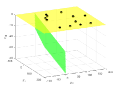
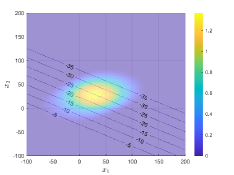
Refer to caption
Refer to caption
Figure 1: Left: the fault Γm~subscriptΓ~m\Gamma_{\tilde{{\itbf m}}} in green and the surface measurement points Pjsubscript𝑃𝑗P_{j} (sketched as black dots on the plane x3=0subscript𝑥30x_{3}=0 which is itself shown in yellow) in the case where M=12𝑀12M=12. Right: the slip 𝒢𝒢{\cal G} on Γm~subscriptΓ~m\Gamma_{\tilde{{\itbf m}}} viewed from above. 𝒢𝒢{\cal G} is taken to be in the direction of steepest descent, so only the magnitude is shown. Depth lines on ΓmsubscriptΓm\Gamma_{\itbf m} are shown.
Refer to caption
Refer to caption
Refer to caption
Refer to caption
Refer to caption
Refer to caption
Figure 2: The data u~~u\tilde{{\itbf u}} at the points Pjsubscript𝑃𝑗P_{j} (represented as circles) for the six inverse problem solved numerically in this paper. Only the horizontal displacements are sketched for clarity. Row 1 to 3: M=12,25,50𝑀122550M=12,25,50. Column 1: low σ𝜎\sigma, column 2: high σ𝜎\sigma.

6.2 Numerical solution to the inverse problem

We computed the posterior probability distribution function ρ(m,C|u~)𝜌mconditional𝐶~u\rho({\itbf m},C|\tilde{{\itbf u}}) given by (4.1-4.2) in each of the 6 cases introduced in the previous section. The prior distribution of mm{\itbf m} was taken to be uniform in the box [1,2]×[1,2]×[100,1]12121001[-1,2]\times[-1,2]\times[-100,-1], and the prior distribution of log10Csubscript10𝐶\log_{10}C was taken to be uniform in [7,2]72[-7,-2]. The computation of ρ(m,C|u~)𝜌mconditional𝐶~u\rho({\itbf m},C|\tilde{{\itbf u}}) was performed using the method of choice sampling, more specifically, we used a modified version of the Metropolis algorithm which is well suited to parallel computing [3]. In [11], section 4, we wrote explicitly a form of this algorithm for computing ρ(m,C|u~)𝜌mconditional𝐶~u\rho({\itbf m},C|\tilde{{\itbf u}}). Note that although the inverse problem considered in [11] was similar to the one studied here, the nonlinear parameter to be reconstructed was different.
The computed marginal posteriors of m=(a,b,d)m𝑎𝑏𝑑{\itbf m}=(a,b,d) are graphed in Figure 3. This figure shows how these computed posteriors tighten around the value of m~~m\tilde{{\itbf m}} as M𝑀M and dimHdimension𝐻\dim H increase as expected from Theorem 4.1. This tightening around the correct value occurs in both low and high σ𝜎\sigma cases and is more narrow in the lower noise case. Deciding that the regularization parameter C𝐶C be a random variable results in a more extensive random walk, however it has the distinct advantage of sweeping through the entire range of values of C𝐶C in the support of the prior of C𝐶C. The computed marginal posteriors of C𝐶C are sketched in Figure 4. This figure illustrates how the algorithm automatically favors optimal values for C𝐶C depending on M𝑀M, dimHdimension𝐻\dim H, and the noise level.

Refer to caption
Refer to caption
Refer to caption
Refer to caption
Refer to caption
Refer to caption
Figure 3: The marginal posteriors of a,b,d𝑎𝑏𝑑a,b,d computed from the data shown in Figure 2 in each of the six cases. Row 1, 2, 3: a,b,d𝑎𝑏𝑑a,b,d. Left column: low noise case. Right column: high noise case. In each figure, the computed posterior for M=12,25,𝑀1225M=12,25, and 50 are sketched.
Refer to caption
Refer to caption
Figure 4: The computed marginal posteriors of the regularization parameter C𝐶C. Left: low noise case. Right: high noise case.

6.3 Failure at fixed C

Fixing a value for the regularization parameter C𝐶C is commonly done in linear inverse problems. Often times, a value for C𝐶C is fixed in such a way that the solution displays satisfactory qualitative features. log10Csubscript10𝐶\log_{10}C is varied linearly until such features appear. Alternatively, one can use more objective criteria for selecting C𝐶C such as the maximum likelihood method, the discrepancy principle, or the generalized cross validation criterion. However, the fault inverse problem is nonlinear in mm{\itbf m}. If one were to apply any of these methods to select a fixed C𝐶C, the selection would depend on mm{\itbf m} and as a result different candidates for mm{\itbf m} would be unfairly compared, [11]. Better results are obtained if we fix the same value for C𝐶C for all mm{\itbf m} in B𝐵B, [12]. Even then, determining the optimal value for C𝐶C is not possible. To illustrate this point, we plotted in Figure 5 the computed posterior marginals assuming various fixed values of the regularization parameter C𝐶C. Qualitatively, it appears that the values 107superscript10710^{-7} and 106superscript10610^{-6} have to be rejected, but it is unclear which of the remaining values is most suitable. This example illustrates that modeling C𝐶C as a random variable and using a Bayesian approach built from the distribution function (4.1-4.2) leads to far superior results.
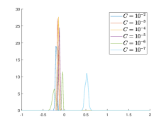
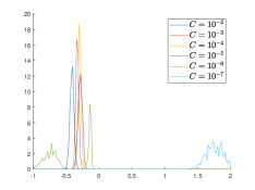
Refer to caption
Refer to caption
Refer to caption
Figure 5: Computed posterior marginals assuming various fixed values of the regularization parameter C𝐶C. First row: a,b𝑎𝑏a,b. Second row: d𝑑d. The computed marginals are only shown for the case M=25𝑀25M=25, low σ.𝜎\sigma.

Funding
This work was supported by Simons Foundation Collaboration Grant [351025].

References

  • [1] A. Aspri, E. Beretta, and A. L. Mazzucato. Dislocations in a layered elastic medium with applications to fault detection. arXiv preprint arXiv:2004.00321, 2020.
  • [2] A. Aspri, E. Beretta, A. L. Mazzucato, and V. Maarten. Analysis of a model of elastic dislocations in geophysics. Archive for Rational Mechanics and Analysis, 236(1):71–111, 2020.
  • [3] B. Calderhead. A general construction for parallelizing metropolis- hastings algorithms. Proceedings of the National Academy of Sciences, 111(49):17408–17413, 2014.
  • [4] N. P. Galatsanos and A. K. Katsaggelos. Methods for choosing the regularization parameter and estimating the noise variance in image restoration and their relation. IEEE Transactions on image processing, 1(3):322–336, 1992.
  • [5] V. Girardin and N. Limnios. Applied probability. From Random Sequences to Stochastic Processes (e-book, Springer, Cham), 2018.
  • [6] I. Gohberg, S. Goldberg, and N. Krupnik. Traces and determinants of linear operators. Integral Equations and Operator Theory, 26(2):136–187, 1996.
  • [7] J. Kaipio and E. Somersalo. Statistical and computational inverse problems, volume 160. Springer Science & Business Media, 2006.
  • [8] R. Kress, V. Maz’ya, and V. Kozlov. Linear integral equations, volume 17. Springer, 1989.
  • [9] Y. Okada. Internal deformation due to shear and tensile faults in a half-space. Bulletin of the Seismological Society of America, vol. 82 no. 2:1018–1040, 1992.
  • [10] D. Volkov. A double layer surface traction free green’s tensor. SIAM Journal on Applied Mathematics, 69(5):1438–1456, 2009.
  • [11] D. Volkov. A parallel sampling algorithm for inverse problems with linear and nonlinear unknowns. arXiv preprint arXiv:2007.05347, 2020.
  • [12] D. Volkov and J. C. Sandiumenge. A stochastic approach to reconstruction of faults in elastic half space. Inverse Problems & Imaging, 13(3):479–511, 2019.
  • [13] D. Volkov, C. Voisin, and I. Ionescu. Reconstruction of faults in elastic half space from surface measurements. Inverse Problems, 33(5), 2017.
  • [14] D. Volkov, C. Voisin, and I. I.R. Determining fault geometries from surface displacements. Pure and Applied Geophysics, 174(4):1659–1678, 2017.