The faint end of the quasar luminosity function at from the Subaru Hyper Suprime-Cam survey
Abstract
We present the quasar luminosity function at derived from the optical wide-field survey data obtained as a part of the Subaru strategic program (SSP) with Hyper Suprime-Cam (HSC). From 81.8 deg2 area in the Wide layer of the HSC-SSP survey, we selected 224 candidates of low-luminosity quasars at by adopting the Lyman-break method down to mag. Based on our candidates and spectroscopically-confirmed quasars from the Sloan Digital Sky Survey (SDSS), we derived the quasar luminosity function at covering a wide luminosity range of mag. We found that the quasar luminosity function is fitted by a double power-law model with a break magnitude of mag. The inferred number density of low-luminosity quasars is lower, and the derived faint-end slope, , is flatter than those of previous studies at . A compilation of the quasar luminosity function at from the HSC-SSP suggests that there is little redshift evolution in the break magnitude and in the faint-end slope within this redshift range, although previous studies suggest that the faint-end slope becomes steeper at higher redshifts. The number density of low-luminosity quasars decreases more rapidly from to than from to .
1 Introduction
Active galactic nuclei (AGNs) release huge radiative energy, which is believed to be powered by the gravitational energy of the accreting medium to supermassive black hole (SMBH) at galactic centers (e.g., Rees, 1984). The mass of SMBHs () in quasars, the most luminous class of AGNs, reaches up to or even higher (e.g., Willott et al., 2010; Shen & Kelly, 2012). Interestingly, such massive SMBHs are seen even at very high redshifts, (e.g., Kurk et al., 2007; Mortlock et al., 2011; Venemans et al., 2013, 2015; Wu et al., 2015; Bañados et al., 2018; Shen et al., 2019; Onoue et al., 2019). The previous studies suggest that the luminous quasars discovered at high redshift have large black hole mass () and accrete mass at the rate close to the Eddington limit. In the local Universe, it has been observationally revealed that there is a tight correlation between the mass of the host bulges () and (e.g., Marconi & Hunt, 2003; Häring & Rix, 2004; Gültekin et al., 2009). This correlation may suggest that SMBHs and their host galaxies have evolved together with close interplay that is now recognized as the galaxy-SMBH coevolution. Therefore, observational studies on the redshift evolution of SMBHs are important not only to understand the evolution of SMBHs, but also to understand the total picture of the galaxy evolution.
The present work focuses on quasars. We refer to luminous, optically selected, unobscured (type-1) AGNs as quasars in our paper. Quasars are important, because (i) they are in the phase of rapid SMBH evolution via active gas accretion, and (ii) their huge luminosity enables us to estimate through spectroscopic observations, even in the very distant Universe. Measurements of the quasar luminosity function (QLF) and black hole mass function in a wide redshift range are a promising approach to reveal the cosmological evolution of SMBHs.
The QLF at has been measured previously over a wide luminosity range (e.g., Siana et al., 2008; Croom et al., 2009; Glikman et al., 2010, 2011; Ikeda et al., 2011; Masters et al., 2012; Ross et al., 2013; Palanque-Delabrouille et al., 2013; Akiyama et al., 2018; Boutsia et al., 2018; Stevans et al., 2018; Adams et al., 2019), leading to the recognition that the QLF is expressed by the broken power-law formula. At , the brighter part of the QLF than knee of the LF has been measured (Richards et al., 2006; Shen & Kelly, 2012; Yang et al., 2016; Jiang et al., 2016; Willott et al., 2010). While the faint side of the QLF at has been established by the Subaru High- Exploration of Low-Luminosity Quasars project (SHELLQs; Matsuoka et al. 2016, 2018a, 2018b, 2018c), the faint side of the QLF at is still controversial (e.g., Ikeda et al., 2012; Matute et al., 2013; McGreer et al., 2013, 2018; Niida et al., 2016). This is because the area and the depth of previous surveys are not enough to measure statistical properties of faint quasar at .
However, the determination of the faint side of the QLF at is important to understand the overall picture of SMBH growth in the early Universe. Previous observations suggest that the number density of luminous quasars increased from the early Universe to and then decreased to the current Universe (e.g., Richards et al., 2006; Croom et al., 2009). It is of particular interest to study possible luminosity dependences of the quasar number-density evolution (luminosity-dependent density evolution; LDDE). Recent optical surveys of high-redshift quasars have reported that low-luminosity quasars show the peak of the number density at lower redshifts than do high-luminosity quasars (e.g., Croom et al., 2009; Ikeda et al., 2011, 2012; Niida et al., 2016). Since the quasar luminosity at a given Eddington ratio corresponds to , the reported LDDE trend is sometimes called the downsizing evolution. The same trend has been found by X-ray surveys for all AGN populations including obscured (type-2) ones (e.g., Ueda et al. 2003, 2014; Hasinger et al. 2005; Miyaji et al. 2015; Aird et al. 2015; see also Enoki et al. 2014; Shirakata et al. 2019 and references therein for theoretical works on the AGN downsizing evolution). Note that the downsizing evolution has been originally proposed to describe the redshift evolution of the galaxy mass function (e.g., Cowie et al., 1996; Neistein et al., 2006; Fontanot et al., 2009). Therefore the AGN downsizing evolution, if present, may provide a significant insight to the galaxy-SMBH co-evolution. However, the number density of low-luminosity quasars at high redshifts has been quite uncertain, which has prevented us from understanding the whole picture of the quasar LDDE. Ueda et al. (2014) noted a possibility that the number ratio of total (type-1 and type-2) low-luminosity AGNs to high luminosity ones may increase from to (“up-down sizing”; see also Glikman et al. 2010, 2011; Giallongo et al. 2015). We need large samples of high- low-luminosity AGNs to examine such scenarios.
The Subaru Strategic Program of the Subaru telescope with the Hyper Suprime-Cam (HSC-SSP; Aihara et al. 2018a) provides an unprecedented dataset to search for low-luminosity quasars at high redshift. The survey started in March 2014 and is assigned 300 nights for 5 years. Taking advantage of the wide field-of-view (FoV) of HSC (a circular FoV with 1.5 deg in diameter; see Miyazaki et al., 2018; Komiyama et al., 2018; Kawanomoto et al., 2018; Furusawa et al., 2018), the Wide-layer component of the HSC-SSP survey will cover 1,400 deg2 when completed, mainly in the equatorial region. The survey depth of the Wide-layer component reaches down to 26.8, 26.4, 26.4, 25.5, and 24.7 AB mags in the , , , , and bands respectively for point sources, which are mag deeper than the Sloan Digital Sky Survey (SDSS; York et al. 2000).
The QLF at and have been derived with the HSC-SSP data by Akiyama et al. (2018) and Matsuoka et al. (2018c), respectively. In this paper, we derive the faint-end of the QLF at with the HSC-SSP data. This paper is organized as follows. The selection criteria adopted in this work are described in Section 2. The survey completeness and contamination are described in Section 3. The derived QLF is shown in Section 4. In Section 5, we compare the derived QLF parameters with those in the literature at and discuss the evolution of the quasar number density. Finally, a summary is presented in Section 6. In the Appendix A, we show the results from our spectroscopic observations for a part of our sample of candidates. Throughout this paper, we adopt a CDM cosmology with , , and the Hubble constant of km s-1 Mpc-1. All magnitudes are described in the AB magnitude system. We use PSF (point-source function) magnitudes for point sources and all the magnitudes are corrected for Galactic extinction based on dust maps by Schlegel et al. (1998).
2 Sample selection
2.1 The HSC Data
We selected quasar candidates from the HSC-SSP survey data. We used the S16A-Wide2 internal release data from the Wide-layer component. The data were reduced with hscPipe-4.0.2 (Bosch et al., 2018). The S16A-Wide2 data cover an area of 339.8 deg2 with all the five bands. However, the edge regions have shallower limiting magnitudes, so we used the full-depth region in the 5 bands in this work. The full-depth regions can be identified with the hscPipe parameter countinputs, which records the number of exposures at a given position for each filter. For the Wide layer data, the full-depth regions correspond to countinputs (4, 4, 6, 6, 6) for (, , , , ) (e.g., Aihara et al., 2018a). In addition, we removed some problematic patches111 “Patch” is a sub-region in HSC images, covering arcmin2. The unit that consists of patches is called “tract” that covers deg2.. In some patches the color sequence of stars shows a significant offset from that computed from the Gunn-Stryker stellar spectrophotometric library (Gunn & Stryker, 1983), because hscPipe is unable to model the PSF accurately for the visits with an extremely good seeing (Aihara et al., 2018b). The offset in each patch is given in the patch_qa table stored in the HSC-SSP database. We removed patches, in which color offset is larger than 0.075 mag either in the vs. , vs. , or vs. color-color plane (see Section 5.8.4 in Aihara et al., 2018a). The Wide layer consists of 7 fields, i.e., GAMA09H, GAMA15H, WIDE12H, XMM-LSS, HECTMAP, VVDS, and AEGIS (Aihara et al., 2018a). Since many patches in the VVDS and a part of the GAMA09H at Decl. deg are affected by the photometric offset problem, we removed all patches in these fields.
Next we created a clean sample with reliable photometry using flags for the 5 bands provided by the hscPipe. First we selected objects detected in all of , , and bands. Then we removed objects, which are affected by saturation, cosmic rays, or bad pixels in the central pixels. We require that the sources are not blended and are in the inner region of a patch and a tract. We also require that an object is not close to bright sources. These flag criteria are listed in Table 1. As a result, 30 million objects were selected as a clean sample in the area of 81.8 deg2. This survey area was estimated by utilizing the HSC-SSP random catalog (Aihara et al., 2018b; Coupon et al., 2018), by counting the number of random points falling on the unflagged area. Thus the incompleteness of the flag selection criteria is taken into account (see Section 3.1 for general treatments of the survey completeness).
Since high-redshift quasars should be observed as point sources, we selected only point sources from the clean sample. For this purpose, we used the second order adaptive moments. We used the adaptive moments measured in the -band, since -band images were preferentially taken under good seeing conditions (0.580.08 arcsec in the Wide layer222 This is slightly larger than the value that Aihara et al. (2018b) reported in their paper (0.56 arcsec). This is because Aihara et al. (2018b) reported the median seeing size for the entire Wide-layer regions while we are focusing only on the full-depth and full-color regions. ). The adaptive moment is measured based on the algorithm of Hirata & Seljak (2003). Our point source criteria are defined with the ratios of the second order adaptive moments to those of the PSF at the position of a given object:
| (1) | |||||
| (2) | |||||
where the indices of “11” and “22” denote the East-West direction and North-South direction, respectively. The completeness and contamination inherent to this selection were evaluated in Akiyama et al. (2018) by comparing the HSC -band measurements with those by the Hubble Space Telescope (HST) Advanced Camera for Surveys (ACS) (see Section 2.2 in Akiyama et al. 2018 and Section 3.2 in this paper for more details). Since (i) the point source selection becomes uncertain for faint objects and (ii) bright objects are saturated, we focus only on objects with where the incompleteness and contamination are low. The above procedure selected 968,997 objects.
| Flag | condition |
|---|---|
| flags_pixel_saturated_center | False |
| flags_pixel_cr_center | False |
| flags_pixel_bad | False |
| flags_pixel_edge | False |
| detect_is_primary | True |
| flags_pixel_bright_object_any | False |
2.2 Color selection
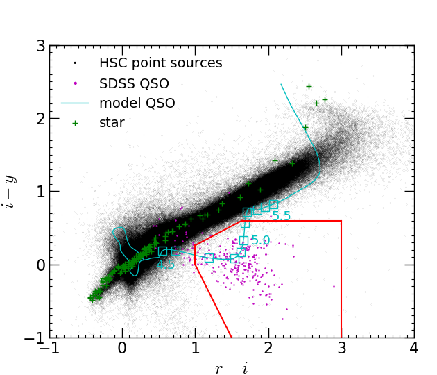
We selected quasar candidates by colors with the following two steps. First we used the two-color diagram of vs. . The colors of the HSC point sources selected in Section 2.1 are shown in Figure 1. Also shown are the colors of stars, which are calculated from stellar spectra of Pickles (1998) with the HSC filter response curves (Miyazaki et al., 2018). The color sequence of the HSC point sources is roughly consistent with that of library stars. We show the color track of a model quasar in Figure 1. This model corresponds to the average spectrum of quasars with , which was derived in Niida et al. (2016) (see also Section 3.1). We also show the colors of SDSS DR12 quasars at (324 objects, selected by the following criteria; , BAL_FLAG = 0, ZWARNING = 0, 0.001, 0.05, SNR_SPEC 1, S/N 3 for , and S/N 5 for and ; see Pâris et al. 2017), whose HSC magnitudes were estimated from the SDSS magnitudes by using Equations (9), (10), and (12) in Akiyama et al. (2018). Our selection criteria of quasar candidates from the HSC point-source sample are:
| (3) | |||||
| (4) | |||||
| (5) | |||||
| (6) |
The criterion of Equation (3) was determined as follows. We fitted the color of HSC point sources with a linear function in the two-color plane. In this process, we only used point sources that satisfy Equation (4) and . To investigate the distribution of the color of galactic stars with removing contamination of point-like galaxies, we imposed Equation (4). Then we calculated their standard deviation and determined the criterion at the 3 separation from the best fit, which corresponds to Equation (3). In addition to this Equation (3), we also adopted Equations (4)–(6) to avoid contaminations by Galactic stars. By these criteria, 613 objects were selected.
In addition, we used color to further remove the remaining sources of contamination, especially at lower redshift. Quasars at have red colors due to the IGM absorption. Based on the color distribution of model quasars, we determined the criterion,
| (7) | |||
| (8) |
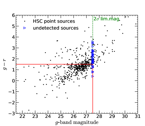
where Equation (7) was determined by checking the color of quasars (see, e.g., Figure 4 in Ikeda et al. 2012). Figure 2 shows a diagram of colors versus -band magnitudes of the HSC point sources selected by Equations (3) – (6). For -undetected objects, we assigned the typical 2 limiting magnitude () in this figure, which satisfies Equation (8). By these criteria we selected 241 objects.
Finally we removed 17 objects by visual inspection. Those 17 objects appear to be significantly affected by artificial features that are related to cosmic rays, tails of bright stars, and so on, which were not perfectly removed by the flags in Table 1. Thus the final candidates of quasars are 224 objects. The sample of our HSC candidates contain no previously-known, spectroscopically-confirmed quasars.
3 Survey completeness and contamination
3.1 Completeness
In order to assess the number density of quasars at , the survey completeness should be evaluated. We estimated the detection completeness and selection completeness as functions of the -band apparent magnitude and the quasar redshift, and then evaluated the survey completeness by combining those two factors. Here the detection completeness is the fraction of quasars that are detected in all of , , and bands in the observed images, while the selection completeness is the fraction of quasars whose color properties with photometric errors satisfy the selection criteria.
For evaluating the completeness, we constructed quasar models as follows (see also Niida et al., 2016; Akiyama et al., 2018). We assumed that the spectral energy distribution (SED) of quasars is independent of the redshift (see, e.g., Kuhn et al., 2001; Telfer et al., 2002; Yip et al., 2004; Jiang et al., 2006; Niida et al., 2016) and also the luminosity (Telfer et al., 2002). We adopted a double power-law continuum (), with a spectral break at Å. The adopted spectral slope at the shorter wavelength side is (Telfer et al., 2002) while that at longer wavelength side is (Vanden Berk et al., 2001). The standard deviation of the slope is assumed to be 0.30 at the both sides (Francis, 1996). Strong emission lines were added to this continuum, assuming Gaussian profiles. Here we included emission lines whose flux is larger than 0.5% of the Ly flux. Since EW of broad emission lines depends on the quasar luminosity in the sense that lower-luminosity quasars have a larger EW (the Baldwin effect; Baldwin, 1977; Kinney et al., 1990; Baskin & Laor, 2004; Nagao et al., 2006), we adopted the luminosity-dependent EWrest(C iv) taken from Table 2 of Niida et al. (2016) and flux ratios given in Table 2 of Vanden Berk et al. (2001). The scatter of EWrest(C iv) is taken into account in the spectral modeling. We also included the Balmer continuum and the Fe ii multiplet emission features by adopting the template given by Kawara et al. (1996). The effects of the intergalactic absorption by neutral hydrogen were incorporated by adopting the opacity models of Inoue et al. (2014), considering the scatter of the hydrogen column density estimated with a Monte Carlo method described in Inoue & Iwata (2008). We constructed 1,000 quasar SED models in each -band magnitude and redshift bin ( mag and ) spanning mag and . In total 441,000 model quasar SEDs were constructed.
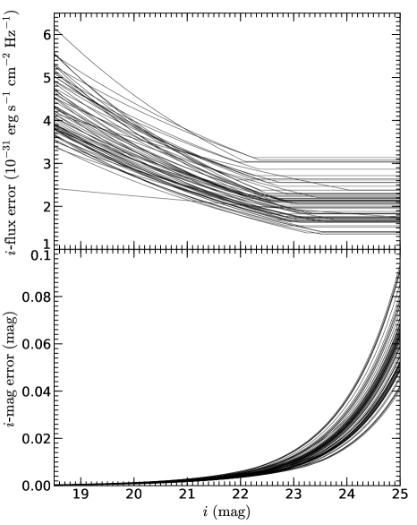
Then we added the photometric error to each magnitude of the model quasars. We investigated the flux errors of real HSC point sources in each of the , , , and bands on randomly selected 62 patches. We fitted a linear function to those flux errors in the logarithmic scale as a function of magnitude in the brighter side (which corresponds to the photon noise), and calculated the average of the flux error in the fainter side (which corresponds to the sky noise). In this calculation we applied clipping in each magnitude bin (mag = 0.2). The results of the fit to the -band photometric error of point sources in each of 62 patches are shown in Figure 3. For each model quasar, photometric error was assigned in each band assuming Gaussian error distribution with the standard deviation estimated above. For each model quasar, we generated 10,000 realizations with different amounts of additional noise.
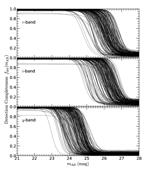
To estimate the detection completeness of quasars, we first investigated the detection completeness of point sources in each of the , and bands. We adopted the same method as described in Aihara et al. (2018b), i.e., artificial point sources were inserted at random positions of the stacked HSC images, and tried to recover them with hscPipe. We ran the simulations for point sources with mag in the randomly selected 62 patches as described above. Then we fitted the derived detection completeness as a function of magnitude in each band with a function of (Serjeant et al., 2000):
| (9) |
where , , , and represent the detection completeness at the brightest and faintest magnitudes, the sharpness of the transition between and , and the magnitude where the detection completeness is 50%, respectively. In most cases, the completeness at the faintest magnitudes () is higher than zero, which is likely due to chance coincidences of input sources with real brighter sources that exist in HSC images. The fitting results for the 62 random patches are shown in Figure 4. In the following, we fixed parameters and to 1.0 and 0.0, respectively.
To evaluate the probability that a quasar is detected in all of the , , and -band images, we multiplied the detection probability of each simulated quasar in , , and -band images. Then we calculated the average of this result for 1,000 model quasars with a certain -band magnitude and redshift. By calculating this average for all model quasars in the ranges of mag and , we obtained the detection completeness of quasars as a function of -band magnitude and redshift. The selection completeness is also estimated as a function of -band magnitude and redshift, by calculating the fraction of model quasars that satisfy our color selection criteria. Finally, by multiplying the detection completeness and selection completeness of quasars, we evaluated the survey completeness as a function of -band magnitude and redshift. This survey completeness is shown in Figure 5. This figure suggests that the survey completeness of our quasar survey is high; the averaged completeness at and mag is 0.87.
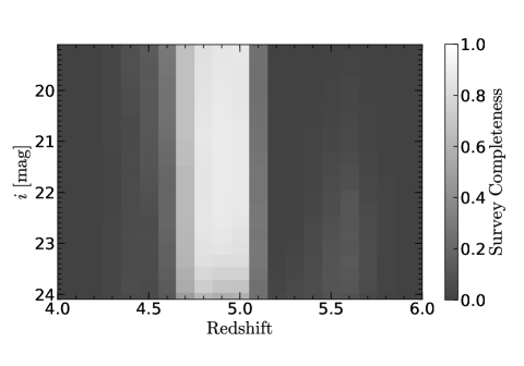
Note that the survey completeness shown in Figure 5 does not include the completeness for the point-source criteria (Equations 1 and 2). As described in Akiyama et al. (2018), the completeness of the point-source criteria is higher than 90% for objects with while it drops to 70% for objects with , when we refer the “best seeing conditions” in Akiyama et al. (2018) (note that the -band images of the HSC-SSP Wide layer were obtained with the seeing size of 0.580.08 arcsec, which is close to the “best seeing conditions (0.5 arcsec)” rather than the “median seeing conditions (0.7 arcsec)” in Akiyama et al. 2018; see Section 2.1). We did not correct for this incompleteness because we fit the QLF only in the range of (see Section 4.2).
3.2 Contamination
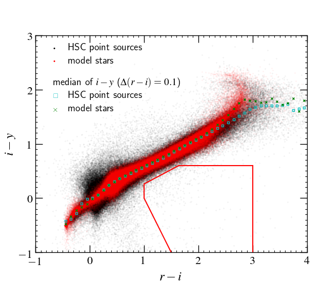
Here we estimate the contamination rate in our photometric sample of quasars. In order to investigate the contamination of Galactic stars, we simulated the number of model stars, which satisfy our color selection criteria. The model stars were constructed by TRILEGAL code, which simulates the number and magnitudes of stars in a given field (Girardi et al., 2005). We adopted an exponential disk model with the default values of scale length and height, and the Chabrier initial mass function (Chabrier et al., 2003). As a result, we got 810,178 model stars. We converted the output Pan-STARRS1 (PS1; Chambers et al., 2016) photometry to the HSC photometry by adopting the color terms, using the coefficients given in Table 2; for example,
(Aihara et al. 2018b; the web page of the HSC-SSP public data release 1 333https://hsc-release.mtk.nao.ac.jp/doc/index.php/data/#color-terms). We added error to the HSC photometry of the model stars in the same way as we did for the model quasars (Section 3.1). The color distribution of the model stars () in the vs. two-color diagram is shown in Figure 6. The color of the real HSC point sources in the same magnitude range is also shown in the figure. The median of the observed and model colors are almost consistent with each other in each bin with , as shown in Figure 6. The color scatter of the HSC point sources is somewhat larger than that of the model stars, which could be possibly due to the underestimate of the HSC photometric error measured by the HSC pipeline as reported in Aihara et al. (2018b). This may lead to the underestimate of the contamination rate, which should be kept in mind in the later analysis. But here we adopt the models of Galactic stars shown in Figure 6. In this case, the number of model stars that meet our color selection criteria is 14 at , while no model stars at satisfy our color selection criteria. Therefore the contamination rate is negligibly small at a brighter range () and moderately low at a fainter range (14/114 12% at ).
Note that, some HSC point sources have photometric errors that are not due to the Gaussian background fluctuation, e.g., cosmic rays. Based on our individual checks, we found that such objects distribute at a distance from the color sequence of Galactic stars in the vs. two-color diagram and partly enter our selection region for quasar candidates. Since such objects are mostly faint () objects, our quasar candidates at may include such objects as contaminations. In addition, as shown in Figure 1 of Akiyama et al. (2018), the contamination rate of compact galaxies that is not spatially resolved in HSC images is almost 0% at , while it increases from 0 to 35% toward . The contamination of such compact galaxies is partly the origin of the difference between the number of HSC point sources (968,997) and the number of model stars (810,178). Compact galaxies in the HSC point-source sample also cause a larger scatter of colors in two-color diagram than the color scatter of model stars seen in Figure 6. For the QLF fitting, we excluded the data at as described later in Section 4.1.
For four objects with in our photometric sample of quasars at , we conducted spectroscopic observations. The observations were carried out with the 4m Blanco telescope at the Cerro Tololo Inter-American Observatory (CTIO) and the Subaru Telescope at the Hawaii Observatory of National Astronomical Observatory of Japan (NAOJ). The details of the spectroscopic observations are described in Appendix A. All of the four observed candidates are confirmed as quasars. This result is consistent with the above estimate that the contamination rate is low, but it should be kept in mind that those four objects are biased toward the brightest objects in our sample of candidates.
| HSC | PS1 | a0 | a1 | a2 |
|---|---|---|---|---|
4 Results
4.1 Binned quasar luminosity function
The numbers of our quasar candidates are summarized in Table 3. For the HSC sample, we assume to infer because it corresponds to the peak of the HSC survey completeness (see Figure 5). The quantities given in this table are corrected for the contamination of Galactic stars, and the following analysis is based on these corrected values. The effective comoving volume of our HSC survey is calculated as
| (11) |
where (81.8 deg2) is the solid angle of our survey and is the survey completeness estimated in Section 3.1. We calculate the number density of the quasars as
| (12) |
where , and is the corrected number of quasars. The uncertainty of the number density is estimated with the Poisson statistics. In the magnitude bins where the corrected number of quasars is lower than 50, we calculate the uncertainty using the statistics presented in Gehrels (1986).
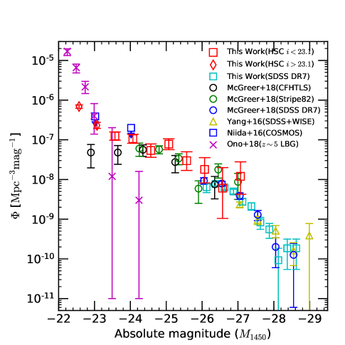
The calculated number densities of quasars and their uncertainties are listed in Table 3 and in Figure 7. Figure 7 also shows the results from previous studies (McGreer et al., 2018; Yang et al., 2016; Niida et al., 2016). Our number densities at are consistent with those reported in the previous studies. At the number densities of Lyman break galaxies (Ono et al., 2018) exceed that of quasars. In this luminosity range, the contamination rate of point-like compact galaxies increases from 0 to 35 % as described in Section 3.2 (see Figure 1 in Akiyama et al., 2018). Therefore our quasar number densities are affected by such point-like galaxies at low-luminosity, and so we exclude the data at from the QLF fitting we describe below.
In order to constrain the bright-end of the QLF, we construct a high-luminosity quasar sample using the spectroscopically-confirmed sample of the SDSS DR7 quasar catalog (Schneider et al., 2010). We select quasars at from the catalog by following the recipe described in Section 4.3 of Akiyama et al. (2018). We select those quasars with SCIENCEPRIMARY and “selected with the final quasar algorithm” based on the TARGET photometry (see Table 1 of Schneider et al., 2010). The effective survey area of the SDSS DR7 sample is 6248 (Shen & Kelly, 2012). The selection completeness is estimated in Richards et al. (2006) as a function of redshift and magnitude. At the selection efficiency is evaluated to be close to % at mag (Figure 6 of Richards et al., 2006). At a given redshift, , we select quasars with as a complete sample with % completeness (see Figure 17 in Richards et al., 2006). We convert to with (appendix B of Ross et al., 2013) and calculate the effective survey volume. The evaluated number densities are shown in Figure 7 and summarized in Table 3. The derived number densities are consistent with those reported in previous studies (McGreer et al., 2018; Yang et al., 2016).
| aaThe numbers of candidates after subtracting the estimated stellar contamination. | bbThe number densities of candidates derived with . | ||
|---|---|---|---|
| (mag) | (mag) | (10-8 Mpc-3 mag-1) | |
| HSC S16A-Wide2 | |||
| 23.85 | 100 | ||
| 23.35 | 38 | ||
| 22.85 | 21 | ||
| 22.35 | 18 | ||
| 21.85 | 9 | ||
| 21.35 | 13 | ||
| 20.85 | 5 | ||
| 20.35 | 3 | ||
| 19.85 | 1 | ||
| 19.35 | 2 | ||
| SDSS DR7 | |||
| 20.30 | 14 | 0.6390.171 | |
| 20.05 | 79 | 0.7720.087 | |
| 19.80 | 68 | 0.6280.076 | |
| 19.55 | 54 | 0.4990.068 | |
| 19.30 | 30 | 0.2770.051 | |
| 19.05 | 23 | 0.2120.044 | |
| 18.80 | 9 | 0.0830.028 | |
| 18.55 | 6 | 0.0550.023 | |
| 18.30 | 1 | 0.00920.0092 | |
| 18.05 | 2 | 0.0180.013 | |
| 17.80 | 2 | 0.0180.013 |
4.2 Double power-law function model
The QLF is known to be well described by a double power-law function
where , , , and are the faint-end slope, the bright-end slope, the normalization of the QLF, and the characteristic absolute magnitude, respectively (e.g., Boyle et al., 2000). The double power-law model is fitted to the above data, using the maximum likelihood method (Marshall et al., 1983). We maximize the likelihood by minimizing , given by
where the sum in the first term is taken over all the HSC and SDSS quasars at . Since the spectroscopic redshift of most objects in our HSC sample is unknown, we probabilistically assign a redshift to each object in our HSC sample whose redshift distribution should follow the survey completeness at the magnitude of each object (Figure 5). We checked that the distribution of assigned redshifts is consistent with the redshift distribution calculated from the best-fit luminosity function described bellow. Therefore this assumption seems to be valid. We then calculate for each quasar based on the assigned redshift. Consequently, for the HSC sample (224 objects with ), the averages with the standard deviations of the assigned redshift and are and , respectively. For the sub-sample used for the QLF fitting (72 objects in ), they are and . For reference, the average and standard deviation of the redshift and for the SDSS spectroscopic sample (288 objects) are and .
The bright-end slope of the QLF at was investigated by McGreer et al. (2013) and Yang et al. (2016). McGreer et al. (2013) used the SDSS DR7 quasar catalog and derived the number densities of quasars with optical color selection. Yang et al. (2016) constructed a sample of bright quasars for a magnitude range of , by combining the SDSS and the Wide-field Infrared Survey Explorer (WISE; Wright et al. 2010) data. The sample of Yang et al. (2016) covers higher luminosities than our sample, and contains a larger number of objects than the McGreer et al. (2013) sample in the brightest range. We fit the number densities of bright quasars at derived by McGreer et al. (2013) and Yang et al. (2016) with a single power-law model. The number densities of Yang et al. (2016) at are corrected to by using the redshift evolution given by Fan et al. (2001). The derived slope is . This slope does not change significantly if we limit the range of the fit to the brighter side () of the data of McGreer et al. (2013) and Yang et al. (2016). Based on this result we fix the bright-end slope to in the following maximum likelihood fitting of the QLF. Since the maximum likelihood fitting need the data of redshift and of each object and , we use our SDSS sample described in Section 4.1, instead of the sample used by McGreer et al. (2013) and Yang et al. (2016).
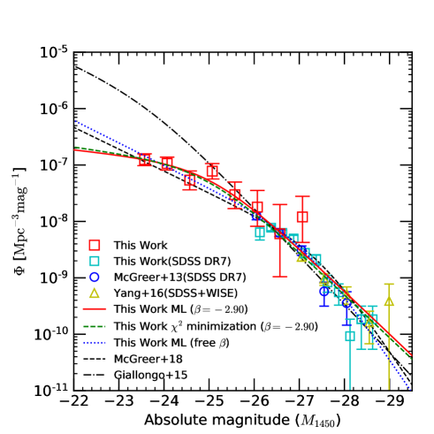
We summarize the results of our maximum likelihood fitting in the first line of Table 4 and adopt these values as our best fit. The derived QLF is shown in Figure 8. The fitting results show a flat faint-end slope, . We also fit the binned luminosity function with a double power-law model through minimization, fixing the bright-end slope to . The best-fit parameters are summarized in the second line of Table 4 and the fitted QLF is shown in Figure 8. The fitting results in these two cases are consistent with each other, and reproduce our HSC number densities reasonably well. We also attempt to fit the QLF by the double power-law model by varying as a free parameter, which resulted in a steeper faint-end slope () as shown in the third line of Table 4.
| [faint-end] | [bright-end] | (10-7 Mpc-3 mag-1) | (mag) | |
|---|---|---|---|---|
| Maximum likelihood (fixed ) | ||||
| minimization (fixed ) | ||||
| Maximum likelihood (free ) |
5 Discussion
5.1 Comparison with previous measurements
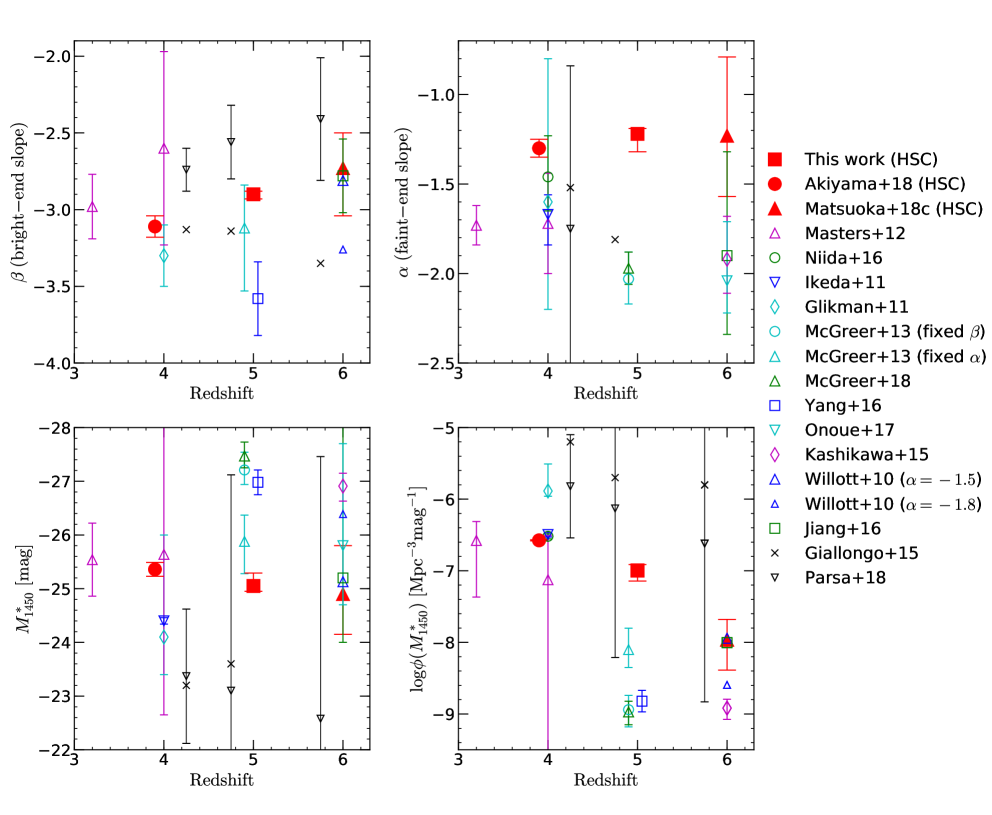
We compare our QLF and previous measurements at in Figures 7 and 8. In Figure 7 our binned QLF is compared with the results of McGreer et al. (2018) using the SDSS, the Stripe82 (Abazajian et al., 2009), and the CFHTLS (Gwyn, 2012) data. The plotted results are consistent with each other at . Though our number densities are systematically higher than those of McGreer et al. (2018) at the fainter magnitudes, both studies indicate a flat faint-end slope. On the other hand, our faint-end slope is flatter than that of Giallongo et al. (2015), , which is based on X-ray detected samples (see Figures 8 and 9).
We also compare the obtained parameters of the QLF with those of previous studies. This is shown in Figure 9. Our bright-end slope is roughly consistent with those in previous studies, because we use essentially the same SDSS sample as used in the previous studies (McGreer et al., 2013, 2018; Yang et al., 2016). On the other hand, our faint-end slope is flatter than that of the previous studies (McGreer et al., 2013, 2018). The reason seems to be that we constructed a larger sample of faint quasars thanks to the deep and wide HSC-SSP survey data (see also Figure 8). The faint-end slope of McGreer et al. (2018) is steeper than ours, presumably because they fixed the bright-end slope to a relatively steep value, (see also Matsuoka et al., 2018c). Our break magnitude is fainter and our number density at the break is higher than those of the previous optical studies.
As a result of the comparison with previous optical surveys at other redshifts, it is inferred that the bright-end slope is roughly constant, and the number density at the break decreases toward higher redshift, in the range of . In previous results except for HSC, the faint-end slope becomes steeper toward higher redshift. Recent measurements with HSC-SSP data, e.g., Akiyama et al. (2018) and SHELLQs (Matsuoka et al., 2016, 2018a, 2018b, 2018c), constructed large low-luminosity quasar samples and reported the flat faint-end slope of the QLF at 4 and 6. Once we focus on the HSC-SSP results, it is indicated that the faint-end slope and the break magnitude are roughly constant for .
5.2 Evolution of the quasar number density
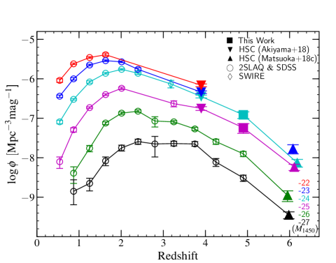
The number density of low-luminosity quasars at high redshifts is a key to understanding luminosity-dependent evolution of quasars and to discuss the cosmological evolution of SMBHs at different masses. Figure 10 shows the quasar number density at different absolute magnitudes as a function of redshift. Based on the quasar luminosity function at derived in Section 4.1, we calculate the quasar number densities at and . These magnitude ranges are not affected by the contamination as described in Section 3.2 and 4.2. At , previous optical studies indicate that the number density of low-luminosity quasars increases toward higher redshift (Glikman et al., 2010, 2011). On the contrary, the HSC results presented in this paper, Akiyama et al. (2018), and Matsuoka et al. (2018c) suggest that the number densities of faint quasars decrease toward high redshift. The reason for the discrepancy between the Glikman et al. (2010, 2011) and present work is unclear, but may be at least in part due to different selection criteria, e.g., the point source separation.
We further explore the density evolution of quasars in the range of . Some recent studies (Jiang et al., 2016; Wang et al., 2019; Yang et al., 2019) reported a more rapid decline in the number density of luminous quasars toward higher redshift at . We fit an exponentially-declining function to the number density of low-luminosity quasars ( and ) evaluated from the HSC survey data,
| (15) |
The derived density evolution parameter ( in Equation 15) for quasars with is at and at . The parameter for quasars with is at and at. Therefore, as seen in luminous quasars (Jiang et al., 2016; Wang et al., 2019; Yang et al., 2019), we confirmed that the number density of low-luminosity quasars decreases more rapidly from to than from to . Though the parameter shows a clear redshift dependence, it does not show a significant luminosity dependence at a fixed redshift range (Figure 10).
6 Summary
This paper presented the QLF at in a wide luminosity range. We constructed a statistical sample of 224 quasars in the magnitude range of , based on the , , , and -band imaging data over 81.8 deg2 taken from the S16A-Wide2 release of the HSC-SSP survey. The quasar candidates were selected by their point-source morphology and -band dropout feature. With estimates of survey completeness and effective area, we calculated the binned QLF. We fitted a double power-law function model to the sample at where the effect of contamination is minimal. The main results of this study are summarized as follows.
- 1.
-
2.
We got the best-fit faint-end slope when the bright-end slope was fixed to . This is flatter than those reported in previous studies at . The break of the double power-law is fainter and the number densities at the break is higher than reported in the previous studies.
-
3.
Combined with the HSC results at and , our results suggest that there is little redshift evolution of the break magnitude and the faint-end slope at . On the other hand, the number density at the break decreases toward high redshift.
- 4.
Appendix A Spectroscopic observations
We conducted spectroscopic observations toward six candidates of quasars as a pilot study for more systematic programs in the future. The targets were selected based on the visibility at the time of observations and their apparent magnitudes. The observations were conducted by the 4m Blanco telescope in the Cerro Tololo Inter-American Observatory (CTIO) and the 8.2m Subaru Telescope of the National Astronomical Observatory of Japan. Among the six objects, four objects meet our latest quasar selection criteria described in this paper, while the remaining two objects do not (see Table 5).
A.1 Subaru Telescope
We observed two faint () objects with the Subaru Telescope, in which one object (J0205–0353) meets our latest quasar selection criteria. The observations were carried out with the Faint Object Camera and Spectrograph (FOCAS; Kashikawa et al., 2002) on 2016 October 7 (S16B-0180S; Niida et al.). We used the 300R grating with the SO58 filter whose wavelength coverage is Å. A width longslit was used, resulting in a wavelength resolution of 900. The seeing size was on average. The individual exposure time was s, and the total exposure time was s for each object.
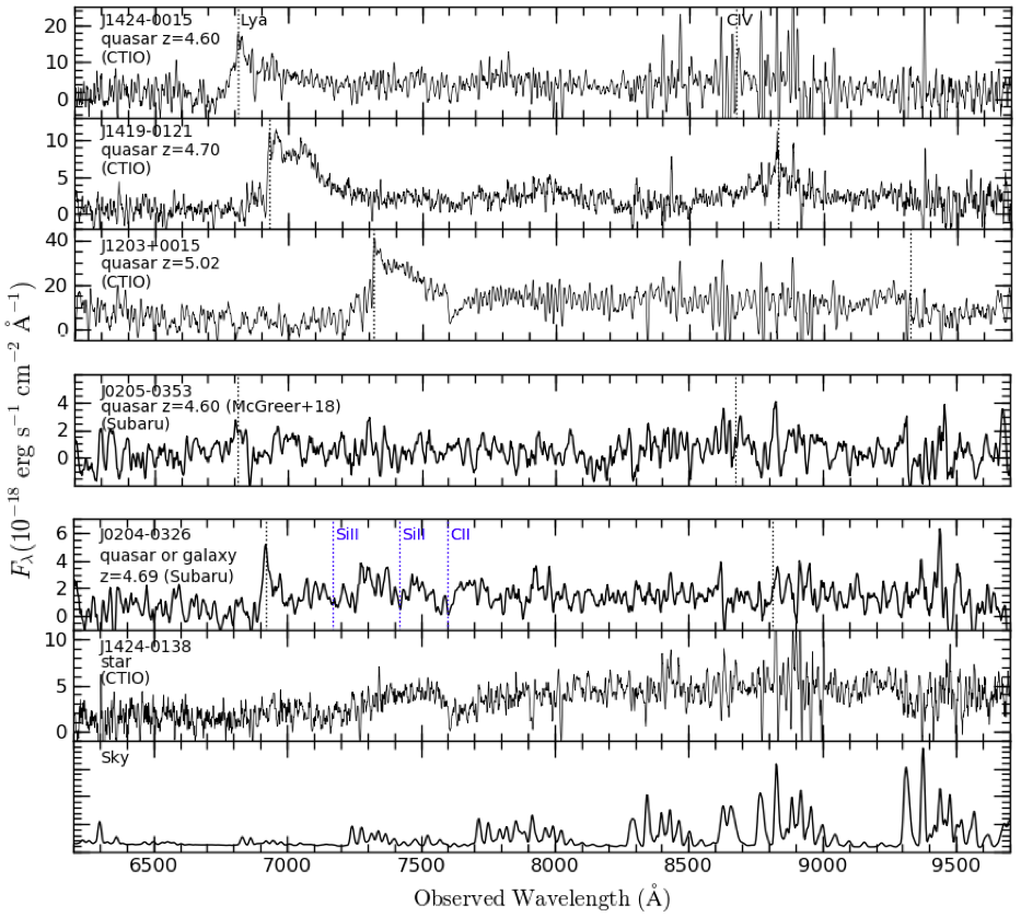
We used IRAF for the data reduction. The flux calibration was tied to a spectrophotometric standard star, Feige 110. The targets are listed in Table 5 and their reduced spectra are shown in Figure 11. J0205–0353 shows only a featureless continuum, while this object was identified as a quasar by McGreer et al. (2018) in a better seeing condition. J0204–0326 shows a relatively narrow Ly emission line, km s-1. This object dose not satisfy the point source selection criteria defined by Equation (2) nor and countinputs , though it satisfies the remaining selection criteria. Its spectrum shows weak features of the interstellar absorption lines of Si ii 1260, Si ii 1304, and C ii 1335, which are shown in Figure 11. Therefore we classified this object as a quasar or galaxy.
| Name | Type | Redshift | Exp. Time (s) | Telescope | ||||
|---|---|---|---|---|---|---|---|---|
| HSC J020435.29–032654.4aa These objects are not selected as quasar candidates by our latest criteria presented in this work. | 23.66 | quasar or galaxy | 4.69 | –22.67 | 2700 | Subaru | ||
| HSC J020541.60–035350.8 | 23.15 | quasar | 4.60bb This redshift is measured by McGreer et al. (2018). | –23.14 | 2750 | Subaru | ||
| HSC J120343.47+001527.4 | 20.61 | quasar | 5.02 | –25.86 | 9900 | CTIO | ||
| HSC J141943.69–012114.6 | 21.61 | quasar | 4.70 | –24.72 | 6300 | CTIO | ||
| HSC J142437.92–001503.0 | 21.35 | quasar | 4.60 | –24.94 | 7200 | CTIO | ||
| HSC J142421.20–013827.3aa These objects are not selected as quasar candidates by our latest criteria presented in this work. | 21.26 | star | 2700 | CTIO |
A.2 CTIO
We observed four bright objects, , with the 4m Blanco telescope at CTIO. Three of them meet our latest quasar selection criteria, while the remaining one does not. The observations were carried out with the Cerro Tololo Ohio State Multi-Object Spectrograph (COSMOS) on 2016 April 12–15 (2016A-0395; Niida et al.). We used the Red VPH Grism with the OG570 filter whose wavelength coverage is Å. A width longslit was used, resulting in a wavelength resolution of 1900. The seeing size was on average. The individual exposure time was s, and the total exposure time was s for each object.
We used IRAF for the data reduction. The flux calibration was tied to spectrophotometric standard stars, Hiltner 600 and LTT 6248. The targets are listed in Table 5 and their reduced spectra are shown in Figure 11. All of the three candidates meeting our latest quasar selection criteria were identified as quasars. The remaining object (J1424–0138) satisfies all the criteria but their and countinputs . It has red continuum and dose not show a Lyman break or broad emission lines. Therefore we conclude that it is a Galactic star.
References
- Abazajian et al. (2009) Abazajian, K. N., Adelman-McCarthy, J. K., Agüeros, M. A., et al. 2009, ApJS, 182, 543
- Adams et al. (2019) Adams, N. J., Bowler, R. A. A., Jarvis, M. J., et al. 2019, arXiv:1912.01626
- Aihara et al. (2018a) Aihara, H., Arimoto, N., Armstrong, R., et al. 2018a, PASJ, 70, S4
- Aihara et al. (2018b) Aihara, H., Armstrong, R., Bickerton, S., et al. 2018b, PASJ, 70, S8
- Aird et al. (2015) Aird, J., Coil, A. L., Georgakakis, A., et al. 2015, MNRAS, 451, 1892
- Akiyama et al. (2018) Akiyama, M., He, W., Ikeda, H., et al. 2018, PASJ, 70, S34
- Baldwin (1977) Baldwin, J. A. 1977, ApJ, 214, 679
- Bañados et al. (2018) Bañados, E., Venemans, B. P., Mazzucchelli, c., et al. 2018, Nature, 553, 473
- Baskin & Laor (2004) Baskin, A., & Laor, A. 2004, ASPC, 311, 175
- Bosch et al. (2018) Bosch, J., Armstrong, R., Bickerton, S., et al. 2018, PASJ, 70, S5
- Boutsia et al. (2018) Boutsia, K., Grazian, A., Giallongo, E., Fiore, F., & Civano, F. 2018, ApJ, 869, 20
- Boyle et al. (2000) Boyle, B. J., Shanks, T., Croom, S. M., et al. 2000, MNRAS, 317, 1014
- Chabrier et al. (2003) Chabrier, G. 2003, PASP, 115, 763
- Chambers et al. (2016) Chambers, K. C., Magnier, E. A., Metcalfe, N., et al. 2016, arXiv:1612.05560
- Coupon et al. (2018) Coupon, J., Czakon, N., Bosch, J., et al. 2018, PASJ, 70, S7
- Cowie et al. (1996) Cowie, L. L., Songaila, A., Hu, E. M., & Cohen, J. G. 1996, AJ, 112, 839
- Croom et al. (2009) Croom, S. M., Richards, G. T., Shanks, T., et al. 2009, MNRAS, 399, 1755
- Enoki et al. (2014) Enoki, M., Ishiyama, T., Kobayashi, M. A. R., & Nagashima, M. 2014, ApJ, 794, 69
- Fan et al. (2001) Fan, X., Strauss, M. A., Schneider, D. P., et al. 2001, AJ, 121, 54
- Fontanot et al. (2009) Fontanot, F., De Lucia, G., Monaco, P., Somerville, R. S., & Santini, P. 2009, MNRAS, 397, 1776
- Francis (1996) Francis, P. J. 1996, PASA, 13, 212
- Furusawa et al. (2018) Furusawa, H., Koike, M., Takata, T., et al. 2018, PASJ, 70, S3
- Gehrels (1986) Gehrels, N. 1986, ApJ, 303, 336
- Giallongo et al. (2015) Giallongo, E., Grazian, A., Fiore, F., et al. 2015, A&A, 578, A83
- Girardi et al. (2005) Girardi, L., Groenewegen, M. A. T., Hatziminaoglou, E., & da Costa, L. 2005, A&A, 436, 895
- Glikman et al. (2010) Glikman, E., Bogosavljević, M., Djorgovski, S. G., et al. 2010, ApJ, 710, 1498
- Glikman et al. (2011) Glikman, E., Djorgovski, S. G., Stern, D., et al. 2011, ApJ, 728, L26
- Gültekin et al. (2009) Gültekin, K., Richstone, D. O., Gebhardt, K., et al. 2009, ApJ, 698, 198
- Gunn & Stryker (1983) Gunn, J. E., & Stryker, L. L. 1983, ApJS, 52, 121
- Gwyn (2012) Gwyn, S. D. J. 2012, AJ, 143, 38
- Häring & Rix (2004) Häring, N., & Rix, H.-W. 2004, ApJ, 604, L89
- Hasinger et al. (2005) Hasinger, G., Miyaji, T., & Schmidt, M. 2005, A&A, 441, 417
- Hirata & Seljak (2003) Hirata, C., & Seljak, U. 2003, MNRAS, 343, 459
- Ikeda et al. (2011) Ikeda, H., Nagao, T., Matsuoka, K., et al. 2011, ApJ, 728, L25
- Ikeda et al. (2012) Ikeda, H., Nagao, T., Matsuoka, K., et al. 2012, ApJ, 756, 160
- Inoue & Iwata (2008) Inoue, A. K., Iwata, I., 2008, MNRAS, 387, 1681
- Inoue et al. (2014) Inoue, A. K., Shimizu, I., Iwata, I., & Tanaka, M. 2014, MNRAS, 442, 1805
- Jiang et al. (2006) Jiang, L., Fan, X., Hines, D. C., et al. 2006, AJ, 132, 2127
- Jiang et al. (2016) Jiang, L., McGreer, I. D., Fan, X., et al. 2016, ApJ, 833, 222
- Kashikawa et al. (2002) Kashikawa, N., Aoki, K., Asai, R., et al. 2002, ApJ, 54, 819
- Kashikawa et al. (2015) Kashikawa, N., Ishizaki, Y., Willott, C. J., et al. 2015, ApJ, 798, 28
- Kawanomoto et al. (2018) Kawanomoto, S., Uraguchi, F., Komiyama, Y., et al. 2018, PASJ, 70, 66
- Kawara et al. (1996) Kawara, K., Murayama, T., Taniguchi, Y., & Arimoto, N. 1996, ApJ, 470, L85
- Kinney et al. (1990) Kinney, A. L., Rivolo, A. R., & Koratkar, A. R. 1990, ApJ, 357, 338
- Komiyama et al. (2018) Komiyama, Y., Obuchi, Y., Nakaya, H., et al. 2018, PASJ, 70, S2
- Kuhn et al. (2001) Kuhn, O., Elvis, M., Bechtold, J., & Elston, R. 2001, ApJS, 136, 225
- Kurk et al. (2007) Kurk, J. D., Walter, F., Fan, X., et al. 2007, ApJ, 669, 32
- Lusso et al. (2012) Lusso, E., Comastri, A., Simmons, B. D., et al. 2012, MNRAS, 425, 623
- Marconi & Hunt (2003) Marconi, A., & Hunt, L. K. 2003, ApJ, 589, L21
- Marshall et al. (1983) Marshall, H. L., Tananbaum, H., Avni, Y., & Zamorani, G. 1983, ApJ, 269, 35
- Masters et al. (2012) Masters, D., Capak, P., Salvato, M., et al. 2012, ApJ, 755, 169
- Matsuoka et al. (2011) Matsuoka, K., Nagao, T., Marconi, A., Maiolino, R., & Taniguchi, Y. 2011, A&A, 527, A100
- Matsuoka et al. (2016) Matsuoka, Y., Onoue, M., Kashikawa, N., et al. 2016, ApJ, 828, 26
- Matsuoka et al. (2018a) Matsuoka, Y., Onoue, M., Kashikawa, N., et al. 2018a, PASJ, 70, S35
- Matsuoka et al. (2018b) Matsuoka, Y., Iwasawa, K., Onoue, M., et al. 2018b, ApJS, 237, 5
- Matsuoka et al. (2018c) Matsuoka, Y., Strauss, M. A., Kashikawa, N., et al. 2018c, ApJ, 869, 150
- Matute et al. (2013) Matute, I., Masegosa, J., Márquez, I., et al. 2013, A&A, 557, A78
- McGreer et al. (2013) McGreer, I. D., Jiang, L., Fan, X., et al. 2013, ApJ, 768, 105
- McGreer et al. (2018) McGreer, I. D., Fan, X., Jiang, L., & Cai, Z. 2018, AJ, 155, 131
- Miyaji et al. (2015) Miyaji, T., Hasinger, G., Salvato, M., et al. 2015, ApJ, 804, 104
- Miyazaki et al. (2018) Miyazaki, S., Komiyama, Y., Kawanomoto, S., et al. 2018, PASJ, 70, S1
- Mortlock et al. (2011) Mortlock, D. J., Warren, S. J., Venemans, B. P., et al. 2011, Natur, 474, 616
- Nagao et al. (2006) Nagao, T., Marconi, A., & Maiolino, R. 2006, A&A, 447, 157
- Neistein et al. (2006) Neistein, E., van den Bosch, F. C., & Dekel, A. 2006, MNRAS, 372, 933
- Niida et al. (2016) Niida, M., Nagao, T., Ikeda, H., et al. 2016, ApJ, 832, 208
- Ono et al. (2018) Ono, Y., Ouchi, M., Harikane, Y., et al. 2018, PASJ, 70, S10
- Onoue et al. (2019) Onoue, M., Kashikawa, N., Matsuoka, Y., et al. 2019, ApJ, 880, 77
- Onoue et al. (2017) Onoue, M., Kashikawa, N., Willott, C. J., et al. 2017, ApJ, 847, L15
- Palanque-Delabrouille et al. (2013) Palanque-Delabrouille, N., Magneville, Ch., Yèche, Ch., et al. 2013, A&A, 551, A29
- Pâris et al. (2017) Pâris, I., Petitjean, P., Ross, N.P., et al. 2017, A&A, 597, 79
- Parsa et al. (2018) Parsa, S., Dunlop, J.S., & McLure, R.J. 2018, MNRAS, 474, 2904
- Rees (1984) Rees, M. J. 1984, ARA&A, 22, 471
- Pickles (1998) Pickles, A. J. 1998, PASP, 110, 863
- Richards et al. (2006) Richards, G. T., Strauss, M. A., Fan, X., et al. 2006, AJ, 131, 2766
- Ross et al. (2013) Ross, N. P., McGreer, I. D., White, M., et al. 2013, ApJ, 773, 14
- Schlegel et al. (1998) Schlegel, D. J., Finkbeiner, D. P., Davis, M., et al. 1998, ApJ, 500, 525
- Schneider et al. (2010) Schneider, D. P., Richards, G. T., Hall, P. B., et al. 2010, AJ, 139, 2360
- Serjeant et al. (2000) Serjeant, S., Oliver, S., Rowan-Robinson, M., et al. 2000, MNRAS, 316, 768
- Shen et al. (2008) Shen, Y., Greene, J. E., Strauss, M. A., et al. 2008, ApJ, 680, 169
- Shen et al. (2011) Shen, Y., Richards, G. T., Strauss, M. A., et al. 2011, ApJS, 194, 45
- Shen & Kelly (2012) Shen, Y., & Kelly, B. C. 2012, ApJ, 746, 169
- Shen et al. (2019) Shen, Y., Wu, J., Jiang, L., et al. 2019, ApJ, 873, 35
- Shirakata et al. (2019) Shirakata, H., Okamoto, T., Kawaguchi, T., et al. 2019, MNRAS, 482, 4846
- Siana et al. (2008) Siana, B., Polletta, M. d. C., Smith, H. E., et al. 2008, ApJ, 675, 49
- Stevans et al. (2018) Stevans, M. L., Fenkelstein, S. L., Wold, I., et al. 2018, ApJ, 863, 63
- Takada et al. (2014) Takada, M., Ellis, R. S., Chiba, M., et al. 2014, PASJ, 66, R1
- Telfer et al. (2002) Telfer, R. C., Zheng, W., Kriss, G. A., & Davidsen, A. F. 2002, ApJ, 565, 773
- Trump et al. (2011) Trump, J. R., Impey, C. D., Kelly, B. C., et al. 2011, ApJ, 733, 60
- Ueda et al. (2003) Ueda, Y., Akiyama, M., Ohta, K., & Miyaji, T. 2003, ApJ, 598, 886
- Ueda et al. (2014) Ueda, Y., Akiyama, M., Hasinger, G., Miyaji, T., & Watson, M. G. 2014, ApJ, 786, 104
- Vanden Berk et al. (2001) Vanden Berk, D. E., Richards, G. T., Bauer, A., et al. 2001, AJ, 122, 549
- Venemans et al. (2013) Venemans, B. P., Findlay, J. R., Sutherland, W. J., et al. 2013, ApJ, 779, 24
- Venemans et al. (2015) Venemans, B. P., Bañados, E., Decarli, R., et al. 2015, ApJ, 801, L11
- Vestergaard &Peterson (2006) Vestergaard, M., & Peterson, B. M. 2006, ApJ, 641, 689
- Wang et al. (2019) Wang, F., Yang, J., Fan, X., et al. 2019, ApJ, 884, 30
- Willott et al. (2010) Willott, C. J., Delorme, P., Reylé, C., et al. 2010, AJ, 139, 906
- Wright et al. (2010) Wright, E. L., Eisenhardt, P. R. M., Mainzer, A. K., et al. 2010, AJ, 140, 1868
- Wu et al. (2015) Wu, X.-B., Wang, F., Fan, X., et al. 2015, Nature, 518, 512
- Yang et al. (2016) Yang, J., Wang, F., Wu, X.-B., et al. 2016, ApJ, 829, 33
- Yang et al. (2019) Yang, J., Wang, F., Fan, X., et al. 2019, ApJ, 871, 199
- Yip et al. (2004) Yip, C. W., Connolly, A. J., Vanden Berk, D. E., et al. 2004, AJ, 128, 2603
- York et al. (2000) York, D. G., Adelman, J., Anderson, Jr., J. E., et al. 2000, AJ, 120, 1579