Prompt photon production in proton collisions as a probe of parton scattering in high energy limit

Abstract

We study the prompt photon hadroproduction at the LHC with the $k_{T}$-factorization approach and the $qg^{*}\to q\gamma$ and $g^{*}g^{*}\to q\bar{q}\gamma$ partonic channels, using three unintegrated gluon distributions which depend on gluon transverse momentum. They represent three different theoretical schemes which are usually considered in the $k_{T}$-factorization approach, known under the acronyms: KMR, CCFM and GBW gluon distributions. We find sensitivity of the calculated prompt photon transverse momentum distribution to the gluon transverse momentum distribution. The predictions obtained with the three approaches are compared to data, that allows to differentiate between them. We also discuss the significance of the two partonic channels, confronted with the expectations which are based on the applicability of the $k_{T}$-factorization scheme in the high energy approximation.

I Introduction

Prompt photon production in hadron collisions is one of the cleanest probes of the strong interactions and the structure of hadrons. Prompt photons are produced in hard partonic scattering and with sufficiently large photon transverse momentum $q_{T}$ and suitable photon isolation criteria, this process may be calculated with high precision in perturbative QCD framework. Since the produced photons do not experience the final state interactions, their cross sections carry information about the properties of incoming partons.

The analysis performed in this study is based on the $k_{T}$-factorization framework Gribov:1984tu ; Catani:1990xk ; Catani:1990eg which is well motivated in the high energy limit. For the prompt photon production at the LHC in the central rapidity region, the high energy limit provides a very good approximation at a lower range of the measured photon transverse momenta. In order to apply the high energy factorization scheme it is necessary that the high energy approximation works. It has been argued that the conditions required to apply the high energy approximation hold in the quasi-multi Regge kinematics, extended for hard processes towards the region of moderate parton momentum fraction $x$ Deak:2008ky ; Motyka:2016lta . In the small $x$ regime, the gluon channel contributions to hadronic cross sections are dominant, and due to an intense gluon radiation, a sizable parton transverse momentum is expected to build up in the QCD radiation process. Within the $k_{T}$-factorization approach, such effects may be treated within all-order resummation schemes like e.g. the Balitsky–Fadin–Kuraev–Lipatov (BFKL) Fadin:1975cb ; Kuraev:1977fs ; Balitsky:1978ic or Catani–Ciafaloni–Fiorani–Marchesini (CCFM) Ciafaloni:1987ur ; Catani:1989sg ; Catani:1989yc ; Marchesini:1994wr schemes. The possibility to investigate the effects of both the all order resummations and large transverse momenta of partons at the tree level parton scattering made this approach vivid and fruitful for phenomenological applications.

The main purpose of this study is to investigate in detail the constraints that the prompt photon production at the Large Hadron Collider (LHC) impose on the transverse momentum dependent gluon distribution $F_{g}(x,\mbox{\boldmath$k$}_{T},\mu_{F})$, computed in the $k_{T}$-factorization framework at small and moderate values of $x$, in wide ranges of the gluon momentum $k_{T}$ and hard factorization scales $\mu_{F}$. This is an important issue since in inclusive cross sections, like e.g. for the Deep Inelastic Scattering (DIS), the gluon transverse momentum is integrated out whereas the photon transverse momentum distribution, $d\sigma^{\gamma}/dq_{T}$, is expected to exhibit significant sensitivity to the transverse momenta of incoming partons. Also the range of scales $\mu_{F}$ probed in the prompt photon production at the LHC is wider than in most processes used for this purpose in the past. Hence, we aim to use the new available precision data from the LHC to better constrain the transverse momentum dependence of the gluon distribution $F_{g}$.

In general terms, a similar approach has already been used in the past Kopeliovich:1995an ; Kopeliovich:1998nw ; JalilianMarian:2012bd ; Benic:2016yqt ; Benic:2016uku ; Benic:2018hvb ; Ducloue:2017kkq ; Baranov:2007np ; Baranov:2008sr ; Lipatov:2011eg ; Lipatov:2016wgr ; Kniehl:2011hc ; Santos:2020nqy ; Goncalves:2020tvh . In the approach proposed in Kopeliovich:1995an ; Kopeliovich:1998nw one considers a fast quark propagating through a color field of a target that scatters by gluon absorption, and a Brehmsstrahlung photon is emitted. In the high energy limit, this process may be represented in a color dipole form Kopeliovich:1995an ; Kopeliovich:1998nw , similarly to the forward Drell–Yan production Brodsky:1996nj . This approach has an advantage to include multiple scattering effects within the framework of the Color Glass Condensate (CGC) McLerran:1993ni ; McLerran:1993ka ; McLerran:1994vd , as it was done in Refs. JalilianMarian:2012bd ; Benic:2016yqt ; Benic:2016uku ; Benic:2018hvb ; Ducloue:2017kkq ; Santos:2020nqy ; Goncalves:2020tvh . Another approach, valid in the single scattering (leading twist) approximation, including effects of the partons’ transverse momenta, was developed in Refs. Baranov:2007np ; Baranov:2008sr ; Lipatov:2011eg ; Lipatov:2016wgr ; Kniehl:2011hc . Calculations made in both the approaches may be divided according to the final state produced in the hard scatter: the prompt photon may be produced in association with one or two jets, and possibly without an accompanying jet, as the incoming partons carry non-zero transverse momentum. The last contribution is, however, suppressed for large transverse momentum of the photon and it is often neglected. Recently, in the framework of CGC, the process of $g^{*}g^{*}\to q\bar{q}\gamma$ was thoroughly studied Benic:2016yqt ; Benic:2016uku ; Benic:2018hvb as the leading one in hadronic and nuclei collisions at large energies, where the large gluon densities at small $x$ contribute.

One of the main goals of this paper is to study in detail the $g^{*}g^{*}$ channel in the single scattering approximation, that is very accurate at larger values of $q_{T}$, and to compare the results with recent data from the LHC. In addition, this analysis is an important step in our ongoing program to constrain the transverse momentum parton distributions with the LHC data, see Ref. Motyka:2016lta for the analysis of the Lam–Tung relation breaking in $Z^{0}$ hadroproduction at the LHC. We improve on the previously known results by carefully comparing two possible realizations of the prompt photon production at the parton level with off-shell gluons $g^{*}$: the $2\to 2$ processes $qg^{*}\to q\gamma$ and ${\overline{q}}g^{*}\to{\overline{q}}\gamma$, and the $2\to 3$ process $g^{*}g^{*}\to q\bar{q}\gamma$. We impose in our analysis the photon isolation criteria of Frixione Frixione:1998jh and use the data from the LHC Aad:2010sp ; Chatrchyan:2011ue ; Aad:2016xcr .

Hence, besides constraining the gluon distribution $F_{g}(x,\mbox{\boldmath$k$}_{T},\mu_{F})$, we also focus on the comparison of two different partonic channels that should be close to each other at the leading logarithmic approximation for small and moderate values of parton momentum fractions $x$. These are already mentioned, the $qg^{*}\to q\gamma$ and $g^{*}g^{*}\to q\bar{q}\gamma$ channels with off-shell gluons. In general, the gluon distribution is larger than the sea quark distributions, and due to larger anomalous dimensions, the gluon distribution is more rapid and drives the evolution of the sea quark sea distributions in scale $\mu_{F}$ and in parton $x$. Hence, one may approximate the sea quarks as coming from the gluon in the last splitting of the parton evolution. This approximation is a basis of a very successful dipole picture of high energy scattering, see e.g. GolecBiernat:1998js ; Golec-Biernat:2017lfv . Thus, one expects that the contribution with sea quarks, $q_{\mathrm{sea}}g^{*}\to q\gamma$, should be well represented as a part of the $g^{*}g^{*}\to q\bar{q}\gamma$ contribution. This should hold true because the amplitude for $g^{*}g^{*}\to q\bar{q}\gamma$ contains diagrams describing the $g^{*}\to q_{\mathrm{sea}}$ splitting in the last step, and in addition subleading terms in the collinear limit. So, in principle one could expect an improved theoretical precision of the hard matrix element in the latter approach. Jumping to the conclusions, to some surprise, we find the opposite to be true. We view this result as an interesting theoretical puzzle and a strong inspiration to perform the complete NLO analysis of the process in the $k_{T}$-factorization framework.

The prompt photon production at the LHC has been thoroughly analyzed within the collinear factorization framework up to the NNLO accuracy Chen:2019zmr . Using this approach, good agreement with the data was found. We do not expect better agreement in our analysis with the $k_{T}$-factorization approach since the process has been treated so far only at the tree level. We rather apply more phenomenologically minded logic to use the theoretically clean observables and precision data in order to refine details of the transverse momentum distribution of partons within the $k_{T}$-factorization framework. Nevertheless, even at the tree level, we find a rather good description of the LHC data in one of the considered scenarios.

The paper is organized as follows. In section II we present the formalism for $qg^{*}\to q\gamma$ and $g^{*}g^{*}\to q\bar{q}\gamma$ channels. In section III we discuss the transverse momentum dependent gluon distributions used in the paper. In section IV we discuss the photon isolation criteria and present our results. We conclude in section V.

II Overview of the process description

We consider the prompt photon production in the $pp$ scattering in the $k_{T}$-factorization approach, depicted in Fig. 1. The incoming proton beam momenta, $P_{1}$ and $P_{2}$, are consider to be light-like: $P_{1}^{2}=P_{2}^{2}=0$ in the high energy approximation: $S=(P_{1}+P_{2})^{2}\gg 4m_{p}^{2}$. The photon kinematics is parametrized with the help of Feynman variable $x_{F}$ and the transverse momentum $\mbox{\boldmath$q$}_{T}$. In the light-cone variables, the real photon momentum in the $pp$ center-of-mass frame reads

$$q_{\gamma}=(q^{+}_{\gamma},q^{-}_{\gamma},\mbox{\boldmath$q$}_{T})=(x_{F}\sqrt{S},\mbox{\boldmath$q$}^{2}_{T}/x_{F}\sqrt{S},\mbox{\boldmath$q$}_{T})\,,$$ (1)

where $q_{\gamma}^{\pm}=q_{\gamma}^{0}\pm q_{\gamma}^{3}$.

At the leading order (LO), the real photon may be produced in the $2\to 2$ partonic channels: $qg\to q\gamma$, ${\overline{q}}g\to{\overline{q}}\gamma$ and $q\bar{q}\to g\gamma$. At the NLO, these $2\to 2$ processes receive one loop correction and the tree level $2\to 3$ processes appear: $gg\to q\bar{q}\gamma$, $qg\to qg\gamma$, $\bar{q}g\to\bar{q}g\gamma$, $qq\to qq\gamma$, $q\bar{q}\to q\bar{q}\gamma$, $\bar{q}\bar{q}\to\bar{q}\bar{q}\gamma$. In our approach, we apply the high energy approximation for all the incoming partons. Since in this regime the gluon density is strongly dominant, it drives evolution of the sea quark densities. Therefore, we shall keep only the contributions with the maximal number of incoming gluons, i.e. $qg\to q\gamma$ and $\bar{q}g\to\bar{q}\gamma$ for the $2\to 2$ processes and $gg\to q\bar{q}\gamma$ for the $2\to 3$ processes.

We apply the $k_{T}$-factorization approach for these processes in which gluons carry non-zero transverse momentum and are off-shell: $g\to g^{*}$. For the incoming quarks and antiquarks, we neglect the transverse momentum and we use the collinear approximation. This setup is often called a hybrid factorization approach. The main motivation for this approximation scheme is our focus on the gluon transverse momentum distribution at small and moderate $x$.

It should be stressed that the available data on the prompt photon hadroproduction at the LHC extend from the kinematic region where the values of parton $x$ are small, $x\sim 0.002$, to larger $x>0.1$. It is well known that the high energy approximation is best motivated in the former region. It was however argued in detail in Refs. Deak:2008ky ; Motyka:2016lta that the high energy factorization scheme may provide a good approximation of the high energy amplitudes also for moderate parton $x$. The key argument used there is based on a detailed analysis of the values of exchanged gluon kinematics in the Sudakov decomposition. In general, the momentum $k$ of the off-shell gluon exchanged in the $t$-channel between the proton with momentum $P_{1}$ and the hard interaction vertex may be written as $k=xP_{1}+\beta P_{2}+k_{\perp}$, where the protons’ momenta $P_{1}$ and $P_{2}$ are approximated to be light-like, and $k_{\perp}$ belongs to the plane orthogonal to $P_{1}$ and $P_{2}$. Then, the quality of the high energy approximation crucially depends on the value of the Sudakov parameter $\beta$ Deak:2008ky ; Motyka:2016lta , which is typically much smaller than the value of parton $x$. These two values are correlated because they both are inversely proportional to the collision energy. The gluon $x$, however, is driven by the large invariant mass of the state produced in the hard collision, while the Sudakov parameter $\beta$ is driven by a usually much smaller mass of the proton remnant. Hence, $\beta\ll x$, and the high energy approximation is still applicable at moderate $x$. For a detailed discussion of this issue and the gauge invariance problem in this approximation scheme for related Drell–Yan and $Z^{0}$ hadroproduction processes, see Ref. Motyka:2016lta .

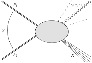
Figure 1: Prompt photon production in proton-proton collisions. The dashed lines represent the photon isolation cone.

II.1 Photon production in the $qg^{*}$ partonic channel

We start the description of the prompt photon hadroproduction in the $k_{T}$-factorization approach with the $2\to 2$ approximation, i.e. with the $qg^{*}\to q\gamma$ and $\bar{q}g^{*}\to\bar{q}\gamma$ channels. In what follows, we use the light cone coordinates of the photon polarization vectors corresponding to helicities $\sigma=\pm$:

$$\epsilon_{(\sigma)}=(0,0,\mbox{\boldmath$\epsilon$}_{\perp}^{(\sigma)}),$$ (2)

where $\mbox{\boldmath$\epsilon$}_{\perp}^{(\pm)}=\mp(1,\pm i)/\sqrt{2}$. The quark–gluon channel contribution to the photon production with rapidity $y$ and transverse momentum $\mbox{\boldmath$q$}_{T}$, derived in Kopeliovich:1995an ; Kopeliovich:1998nw ; Motyka:2014lya , reads

$$\frac{d\sigma^{(qg^{*}\to q\gamma)}_{\sigma}}{dy\,d^{2}\mbox{\boldmath$q$}_{T}} =\frac{4\pi\alpha_{\mathrm{s}}(\mu_{R})}{3}\int_{x_{F}}^{1}dx_{q}\sum_{i\in\{f,\bar{f}\}}e_{i}^{2}\,q_{i}(x_{q},\mu_{F})$$

$$\times\int{d^{2}\mbox{\boldmath$k$}_{T}\over\pi{k}_{T}^{2}}\,F_{g}({x}_{g},{k}_{T},\mu_{F})\;\tilde{\Phi}_{\sigma\sigma}(\mbox{\boldmath$q$}_{T},\mbox{\boldmath$k$}_{T},x_{F}/x_{q}),$$ (3)

where $k_{T}=|\mbox{\boldmath$k$}_{T}|$, $e_{i}$ are quark charges in units of the elementary charge $e$, $q_{i}$ are collinear distributions of quarks and antiquarks with flavors $f$ and $\bar{f}$ (not multiplied by $x$). In addition, the photon Feynman variable reads

$$x_{F}=\frac{q_{T}}{\sqrt{S}}\,e^{y},$$ (4)

while the gluon momentum fraction $x_{g}$ is obtained from kinematics of the parton scattering in the high energy limit

$$x_{g}=\frac{q_{T}}{\sqrt{S}}\,e^{-y}+\frac{z(\mbox{\boldmath$k$}_{T}-\mbox{\boldmath$q$}_{T})^{2}}{(1-z)q_{T}\sqrt{S}}\,e^{-y},$$ (5)

where $z=x_{F}/x_{q}$. From now on, we keep the renormalization and factorization scales to be equal, $\mu_{R}=\mu_{F}$.

The function $F_{g}$ is the transverse momentum dependent (or unintegrated) gluon density, in the form fixed by the leading logarithmic relation to the collinear gluon density $g(x,\mu_{F})$:

$$\int_{0}^{\mu_{F}^{2}}d{k}_{T}^{2}\,F_{g}(x,{k}_{T},\mu_{F})=xg(x,\mu_{F}).$$ (6)

All quarks are assumed to be massless when compared to the photon transverse momentum $q_{T}$. The diagonal in photon helicity impact factors are given by

$$\tilde{\Phi}_{\sigma\sigma}(\mbox{\boldmath$q$}_{T},\mbox{\boldmath$k$}_{T},z)=\sum_{\lambda_{1},\lambda_{2}\in\{+,-\}}\ {A_{\lambda_{1},\lambda_{2}}^{(\sigma)}}^{\dagger}A_{\lambda_{1},\lambda_{2}}^{(\sigma)}\,,$$ (7)

where $\lambda_{1}$ and $\lambda_{2}$ are helicities of the incoming and outgoing quark, respectively. With the chosen photon polarization vectors (2), the functions

$$A_{\lambda_{1},\lambda_{2}}^{(\pm)}=\frac{e}{8\pi}\,\delta_{\lambda_{1},\lambda_{2}}\,(2-z\mp\lambda_{1}z)\left[\frac{-\mbox{\boldmath$q$}_{T}}{\mbox{\boldmath$q$}_{T}^{\ 2}}-\frac{-(\mbox{\boldmath$q$}_{T}-z\mbox{\boldmath$k$}_{T})}{(\mbox{\boldmath$q$}_{T}-z\mbox{\boldmath$k$}_{T})^{2}}\right]\cdot\mbox{\boldmath$\epsilon$}_{\bot}^{\ (\pm)}$$ (8)

are proportional to the photon emission amplitudes. After summation over quark and photon helicities, the cross section for the real photon hadroproduction reads

$$\frac{d\sigma^{\gamma}}{dyd^{2}\mbox{\boldmath$q$}_{T}} =\frac{\alpha_{\mathrm{em}}}{3\pi}\int_{x_{F}}^{1}\frac{dz}{z}\,\frac{x_{F}}{z}\,\sum_{i\in\{f,\bar{f}\}}e_{i}^{2}\,q_{i}\!\left(\frac{x_{F}}{z},\mu_{F}\right)$$

$$\times\int\frac{d^{2}\mbox{\boldmath$k$}_{T}}{k_{T}^{2}}\alpha_{s}F_{g}({x}_{g},k_{T},\mu_{F})\,\frac{\left[1+(1-z)^{2}\right]z^{2}\mbox{\boldmath$k$}_{T}^{2}}{\mbox{\boldmath$q$}_{T}^{\ 2}(\mbox{\boldmath$q$}_{T}-z\mbox{\boldmath$k$}_{T})^{2}}\,+(y\rightarrow-y),$$ (9)

where the symmetrization $y\rightarrow-y$ since both the initial states, $q(k_{1})\,g^{*}(k_{2})$ and $g^{*}(k_{1})\,q(k_{2})$, contribute.

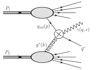
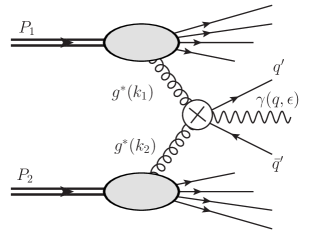
a)	b)

Figure 2: Partonic channels in $\gamma$ hadroproduction: a) the $q_{\mathrm{val}}g^{*}\to q\gamma$ channel and b) the $g^{*}g^{*}\to q\bar{q}\gamma$ channel. The crossed blobs represent channel dependent hard scattering amplitudes.

The integrand in (9) is singular for $\mbox{\boldmath$q$}_{T}=z\mbox{\boldmath$k$}_{T}$. This is a collinear singularity coming from the emitted photon momentum parallel to the outgoing quark momentum. In experiments, however, the photon measurement requires a separation from the outgoing hadrons (or jets). Hence, the experimental data assume certain isolation cut, $\Theta_{R_{\gamma}}(q_{\gamma},\{p^{H}_{i}\})$, which depends on the photon momentum $q_{\gamma}$, the hadron momenta $\{p^{H}_{i}\}$ and the isolation cone parameter $R_{\gamma}$. In the parton level formulas, the isolation criterion is implemented with outgoing parton momenta $\{p_{i}\}$ instead of the hadronic momenta $\{p^{H}_{i}\}$. Thus, in order to obtain a physically meaningful result, Eq. (9) must be complemented by a suitable cut $\Theta_{R_{\gamma}}(\mbox{\boldmath$q$}_{T},z,\mbox{\boldmath$k$}_{T})$. The detailed discussion of our implementation is given section (IV.1).

The $qg^{*}\to q\gamma$ channel described in the high energy limit within the $k_{T}$-factorization framework was shown Kopeliovich:1995an ; Kopeliovich:1998nw to be equivalent to the dipole picture of high energy scattering, in close analogy to the dipole picture of the Drell–Yan process Kopeliovich:1995an ; Kopeliovich:1998nw ; Brodsky:1996nj , see also Motyka:2014lya ; Brzeminski:2016lwh for recent developments. This picture is obtained by the Fourier transform of the impact factors to the impact parameter space, and the color dipole scattering amplitude emerges as a result of an interference between the initial and final state photon emission amplitudes. This approach has an advantage to be capable to efficiently include the effects of multiple scattering and it was explored for instance in recent analyses Santos:2020nqy ; Goncalves:2020tvh .

II.2 Photon production in the $g^{*}g^{*}$ partonic channel

In an alternative approach to the prompt photon production in the high energy approximation, one generates sea quarks from the gluon in the last splitting. With this assumption, the sea quark contributions $q_{\rm sea}$ can be absorbed into the $g^{*}g^{*}\to q\bar{q}\gamma$ hard matrix elements. The valence quark contribution $q_{\mathrm{val}}$, however, is not included in the $g^{*}g^{*}$ channel, and these two contributions enter the cross section additively, see Fig. 2,

$$d\sigma^{\gamma}=d\sigma^{(q_{\mathrm{val}}g^{*}\to q\gamma)}+d\sigma^{(g^{*}g^{*}\to q\bar{q}\gamma)}.$$ (10)

The $g^{*}g^{*}\to q\bar{q}\gamma$ hard subprocesses cross section is calculated in the $k_{T}$-factorization framework. The scheme and details of the calculations follow closely more general calculations performed in the same setup for the Drell–Yan structure functions Motyka:2016lta . In fact, the formulas for the photon production may be recovered from those derived in Ref.  Motyka:2016lta by removing leptonic part with boson propagator, taking the limit $M\to 0$ for the Drell–Yan intermediate boson mass and considering only the diagonal in helicity structure functions for the transverse polarizations. For completeness, we shortly repeat the main steps of these calculations adjusted to the photon hadroproduction case.

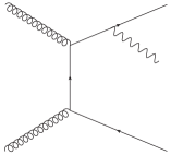
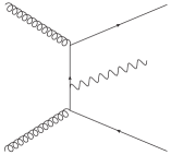
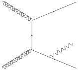
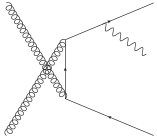
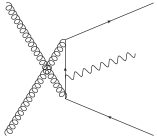
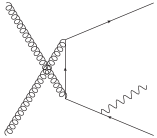
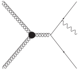
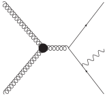
Figure 3: Eight Feynman diagrams that contribute to the $g^{*}g^{*}\to q\bar{q}\gamma$ partonic channel corresponding to the amplitudes ${\cal M}^{(i)}$ for $i=1,2,\ldots,8$, respectively. The black blobs denote the effective triple gluon vertex $V_{\mathrm{eff}}$, see Appendix of Ref. Motyka:2016lta for its definition.

In the $k_{T}$-factorization gluons are virtual, $k_{i}^{2}\simeq-\mbox{\boldmath$k$}_{iT}^{2}<0$, and quarks are taken to be massless, $p^{2}_{3}=p_{4}^{4}=0$. The standard gluon momenta decomposition in the high energy limit is applied: $k_{1}=x_{1}P_{1}+k_{1\,\perp}$ and $k_{2}=x_{2}P_{2}+k_{2\,\perp}$, see also the discussion in Sec. II, preceding Sec. II.1. The parton level scattering amplitude is a sum of eight diagrams shown in Fig. 3. The high energy limit for virtual gluon polarizations is used, in which the virtual gluon polarization vectors $\pi_{g^{*}}(k_{i})$ are approximated by the so-called “nonsense polarizations”, using the so-called Collins–Ellis trick Collins:1991ty in the derivations,

$$\pi^{\mu}_{g^{*}}(k_{1})\simeq x_{1}P^{\mu}_{1}/\sqrt{\mbox{\boldmath$k$}_{1T}^{2}}\,,~{}~{}~{}~{}~{}~{}~{}~{}~{}~{}~{}~{}\pi^{\mu}_{g^{*}}(k_{2})\simeq x_{2}P^{\mu}_{2}/\sqrt{\mbox{\boldmath$k$}_{2T}^{2}}\,.$$ (11)

The impact factors ${\cal T}_{\mu}^{(i)}$ with $i=1,2,\ldots,8$ are defined as

$${\cal T}_{\mu}^{(i)}={\cal M}^{(i)}_{\mu,\alpha\beta}\,P_{1}^{\alpha}P_{2}^{\beta},$$ (12)

where ${\cal M}^{(i)}_{\mu,\alpha\beta}$ are the amplitudes for the diagrams shown in Fig. 3 with amputated polarization vectors of the incoming gluons and outgoing photon. The explicit expressions for the impact factors are given in Appendix of Ref. Motyka:2016lta .

The $g^{*}g^{*}\to q\bar{q}\gamma$ impact factor, given by ${\cal T}^{g^{*}g^{*}}_{\mu}=\sum_{i=1}^{8}{\cal T}^{(i)}_{\mu}$, is used to calculate the $g^{*}g^{*}$ channel contributions cross sections for photon production with helicity $\sigma$,

$$d\sigma^{(g^{*}g^{*}\to q\bar{q}\gamma)}_{\sigma} =\int dx_{1}\int{d^{2}\mbox{\boldmath$k$}_{1T}\over\pi{k}_{1T}^{2}}F_{g}(x_{1},{k}_{1T},\mu_{F})\int dx_{2}\int{d^{2}\mbox{\boldmath$k$}_{2T}\over\pi{k}_{2T}^{2}}F_{g}(x_{2},{k}_{2T},\mu_{F})$$

$$\times\;{(2\pi)^{4}\over 2S}\,{\cal H}_{\sigma}\,dPS_{3}(k_{1}+k_{2}\to p_{3}+p_{4}+q),$$ (13)

with $F_{g}$ being the unintegrated gluon distribution introduced in the previous section and

$${\cal H}_{\sigma}=\sum_{f\in\{u,d,s,c,b\}}{1\over(N_{c}^{2}-1)^{2}}\sum_{a,b}\sum_{i_{3},i_{4}}\sum_{r_{3},r_{4}}\left({\cal T}^{g^{*}g^{*}}_{\mu}\epsilon^{\mu}_{(\sigma)}\right)\left({\cal T}^{g^{*}g^{*}}_{\nu}\epsilon^{\nu}_{(\sigma)}\right)^{\dagger},$$ (14)

where summations are performed over quark flavors $f$ (present through the charge $e_{f}$ in the amplitudes ${\cal T}^{g^{*}g^{*}}_{\mu}$), color indices of the gluons $(a,b)$ and quarks $(i_{3},i_{4})$, and over the quark helicities $(r_{3},r_{4})$. The latter summation leads to traces over Dirac spinors which are evaluated with the FORM program for symbolic manipulations Vermaseren:2000nd . The resulting expressions, obtained in two independent calculations, are lengthy and do not need to be explicitly displayed. It was also checked that ${\cal H}_{\sigma}\sim{k}_{iT}^{2}$ when the gluon transverse momentum ${k}_{iT}^{2}\to 0$, as required by the gauge invariance condition in the high energy limit.

The phase space for the final state particles of partonic scattering is parametrized in terms of the photon variables $(y,\mbox{\boldmath$q$}_{T})$ and the variables $(z,\phi_{\kappa})$ describing the $q\bar{q}$ kinematic configuration,

$$dPS_{3}(k_{1}+k_{2}\to p_{3}+p_{4}+q)={dy\,d^{2}\mbox{\boldmath$q$}_{T}\,dz\,d\phi_{\kappa}\over 8(2\pi)^{9}}d\kappa^{2}$$ (15)

$$\times\,\delta\!\left[\kappa^{2}-z(1-z)\!\left(x_{q\bar{q}}x_{2}S-x_{q\bar{q}}\frac{q_{T}^{2}}{x_{F}}-\mbox{\boldmath$\Delta$}^{2}\right)\right],$$

where the variables $(z,\mbox{\boldmath$\kappa$})$ are implicitly defined by the parametrization of the quark and antiquark momenta

$$p_{3}=zx_{q\bar{q}}P_{1}+{\mbox{\boldmath$p$}_{3}^{2}\over zx_{q\bar{q}}S}P_{2}+p_{3\perp},\qquad p_{4}=(1-z)x_{q\bar{q}}P_{1}+{\mbox{\boldmath$p$}_{4}^{2}\over(1-z)x_{q\bar{q}}S}P_{2}+p_{4\perp},$$ (16)

in which

$$p_{3\perp}=(0,0,\mbox{\boldmath$p$}_{3}),\quad p_{4\perp} =(0,0,\mbox{\boldmath$p$}_{4}),\quad\mbox{\boldmath$p$}_{3}=z\mbox{\boldmath$\Delta$}+\mbox{\boldmath$\kappa$},\quad\mbox{\boldmath$p$}_{4}=(1-z)\mbox{\boldmath$\Delta$}-\mbox{\boldmath$\kappa$},$$

$$\Delta =\mbox{\boldmath$k$}_{1}+\mbox{\boldmath$k$}_{2}-\mbox{\boldmath$q$},\quad x_{q\bar{q}}=x_{1}-x_{F}.$$ (17)

For the comparison with data it is necessary to integrate over the final state quark/antiquark kinematical variables and sum over the photon polarizations,

$${d\sigma^{\gamma}\over dyd^{2}\mbox{\boldmath$q$}_{T}}=\int dz\int d\phi_{\kappa}\,\sum_{\sigma=\pm}{d\sigma^{(g^{*}g^{*}\to q\bar{q}\gamma)}_{\sigma}\over dyd^{2}\mbox{\boldmath$q$}_{T}dzd\phi_{\kappa}}.$$ (18)

III Transverse momentum dependent gluon distributions

Several parametrizations of the transverse momentum dependent gluon distribution in the proton, $F_{g}(x,{k}_{T},\mu_{F})$, were proposed. Many of them were derived in the regime of small-$x$ dynamics, including solutions of the BFKL equation Fadin:1975cb ; Kuraev:1977fs ; Balitsky:1978ic or the Balitsky–Kovchegov (BK) Balitsky:1995ub ; Kovchegov:1999yj ; Kovchegov:1999ua equation. The data for the prompt photon production, however, extend out of the small-$x$ domain. Therefore, we consider parametrizations that may be used also for moderate values of $x>0.01$. The most widely used approaches having this feature are the following:

• The Kimber–Martin–Ryskin (KMR) approach Kimber:1999xc ; Kimber:2001sc that permits to recover the unintegrated parton distributions from the collinear parton distribution functions.

• The approach based on the solutions of the CCFM equation Ciafaloni:1987ur ; Catani:1989sg ; Catani:1989yc ; Marchesini:1994wr , implemented by Jung and Hansson (JH) Hansson:2003xz and later on by Jung and Hautmann (JH-2013) Hautmann:2013tba .

• We also consider the gluon distribution from the Golec-Biernat–Wüsthoff (GBW) model GolecBiernat:1998js , extended phenomenologically to the values of $x>0.01$.

All of these parametrizations were optimized to describe the HERA data on the proton structure function $F_{2}$ (for the GBW gluon distribution, the optimization was performed for $x\leq 0.01$ but not for its phenomenological extension).

III.1 KMR-AO gluon distribution

The KMR scheme was used in several variations. Our choice is the integral version of the KMR prescription Golec-Biernat:2018hqo in which the unintegrated gluon distribution for $k_{T}>Q_{0}=1~{}{\rm GeV}$ is given by

$$F_{g}(x,{k_{T}},Q)\equiv\frac{T_{a}(Q,{k_{T}})}{{k_{T}}^{2}}\sum_{a^{\prime}\in\{f,\bar{f},g\}}\int_{x}^{1-\Delta({k_{T}},Q)}\frac{dz}{z}\,P_{ga^{\prime}}(z,{k_{T}})\,D_{a^{\prime}}\Big{(}\frac{x}{z},{k_{T}}\Big{)}\,,$$ (19)

where the function $T_{a}$ is called the Sudakov form factor

$$T_{g}(Q,{k_{T}})=\exp\left\{-\int_{k^{2}_{T}}^{Q^{2}}\frac{dp_{T}^{2}}{p_{T}^{2}}\sum_{a^{\prime}\in\{f,\bar{f},g\}}\int_{0}^{1-\Delta(p_{T},Q)}dzzP_{a^{\prime}g}(z,p_{T})\right\}\,.$$ (20)

In the above, $f/\bar{f}$ denote quark/antiquark flavors, $P_{aa^{\prime}}(z,\mu)$ are the Altarelli–Parisi splitting functions given in terms of the expansion in $\alpha_{s}(\mu)/(2\pi)$ and $D_{a}(x,\mu)$ are collinear parton distribution functions (PDFs). We choose the leading order splitting functions and the CT10 PDFs Lai:2010vv . We consider the angular ordering version of the KMR distribution (KMR-AO) in which the function $\Delta$ in the upper integration limits equals

$$\Delta({k_{T}},Q)=\frac{{k_{T}}}{{k_{T}}+Q}\,.$$ (21)

This prescription imposes angular ordering in the last step of the evolution Kimber:2001sc . For the values $k_{T}\leq Q_{0}$, the unintegrated gluon distribution is frozen at the boundary value $F_{g}(x,Q_{0},Q)$.

We prefer to use the integral version of the KMR distribution over the differential one since it allows to avoid problems for large values of transverse momentum, $k_{T}>Q$, discussed in Golec-Biernat:2018hqo .

III.2 JH and JH-2013 gluon distribution

The unintegrated gluon distribution in the all-loop CCFM scheme Marchesini:1994wr ; Hautmann:2017fcj ; Golec-Biernat:2019scr takes into account small-$x$ coherence effects which are reflected in angular ordering in gluon cascade branching. This leads to a non-Sudakov form factor which screens the $1/z$ singularity in the $P_{gg}$ splitting function. The CCFM scheme was extended for gluons to the region of large $x$ by taking into account terms with finite $z$ in $P_{gg}$, and the Sudakov form factor with angular ordering of the final state emissions. Infrared parameters in such a scheme were fitted to the HERA data on $F_{2}$ by Jung and Hansson in Hansson:2003xz , which analysis offers the JH unintegrated gluon distribution. Along similar lines in the year 2013 a new parametrization (called JH-2013) of the unintegrated gluon distribution was constructed by Jung and Hautmann Hautmann:2013tba . The new parametrization is based on the angular ordered CCFM gluon branching scheme with unintegrated valence quark distributions included.

III.3 Extended GBW gluon distribution

The unintegrated gluon density $F_{g}$ from the GBW saturation model is given by

$$\alpha_{s}F_{g}(x,k_{T},\mu)=\frac{3\sigma_{0}}{4\pi^{2}}\frac{k_{T}^{2}}{Q_{s}^{2}}\exp(-k_{T}^{2}/Q_{s}^{2})\times\left(\frac{1-x}{1-0.01}\right)^{7}\;,$$ (22)

where the the saturation scale $Q^{2}_{s}=(x/x_{0})^{-\lambda}~{}{\rm GeV}^{2}$. We use the parameters from the recent refit of the GBW model done in Golec-Biernat:2017lfv : $\sigma_{0}=27.32~{}{\rm mb}$, $x_{0}=0.42\cdot 10^{-4}$ and $\lambda=0.248$. Since the GBW model was fitted to the data with $x<0.01$, the original form of the gluon distribution was extrapolated to the values of $x>0.01$ by multiplying by the factor $(1-x)^{7}/(1-0.01)^{7}$, that ensures a smooth transition from the small-$x$ domain to the region of $x\sim 1$. The form of the distribution for $x\to 1$ follows from dimensional scaling rules of the Regge formalism close to the kinematic end point. The main purpose of using the extrapolated GBW gluon distribution is its distinct transverse momentum dependence that is exponentially suppressed for $k_{T}>1~{}{\rm GeV}$. Such a strong and narrow in $k_{T}$ suppression is not present in the KMR-AO and JH gluon distributions.

III.4 Gluon distribution comparison

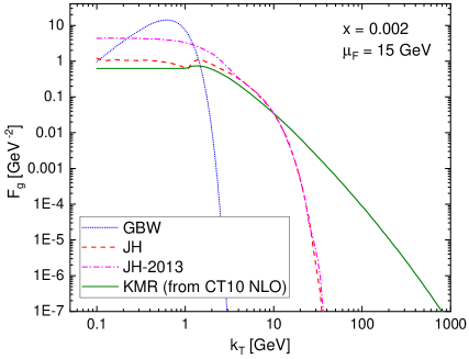
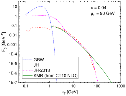
Figure 4: Four unintegrated gluon distributions $F_{g}(x,{k_{T}},\mu)$ (see the text) as a function of gluon transverse momentum $k_{T}$ for two indicated values of gluon $x$ and factorization scales $\mu_{F}$. In the computation of the GBW gluon distribution, the leading order running $\alpha_{s}=\alpha_{s}(\mu_{F})$ was used.

In Fig. 4, we illustrate the properties of the considered unintegrated gluon distributions, which are shown as a function of gluon transverse momentum $k_{T}$ for two values of the longitudinal momentum fraction, $x=0.002$ and $0.04$, and two values of the factorization scale, $\mu_{F}=15$ and 90 GeV, correspondingly. They are motivated by typical values in the prompt photon production at the LHC in the central region when $\mu_{F}=q_{T}$. Clearly, the GBW distribution is much narrower and strongly peaked at small $k_{T}$ than other distributions, which are similar in the region $Q_{0}=1~{}{\rm GeV}<k_{T}<\mu_{F}$ but differ at the ends of the $k_{T}$ spectrum. In particular, while the KMR and JH distributions are almost the same for $k<Q_{0}$, the new distribution JH-2013 is significantly higher. On the other hand, while the JH and JH-2013 distributions are practically the same for $k_{T}\gg\mu_{F}$, they are much more strongly suppressed than the KMR distribution which decreases much slower, approximately as a moderate negative power of $k_{T}$. These distinct $k_{T}$-shapes should have an important impact on the predictions of the measured photon distribution in transverse momentum $q_{T}$.

We also compare the $x$-dependence of the gluon distributions. We choose to illustrate this dependence by evaluating the ‘collinear integral’ of the unintegrated gluon distributions

$$\widetilde{xg}(x,\mu_{F}^{2})=\int_{0}^{\mu_{F}^{2}}dk_{T}^{2}\,F_{g}(x,k_{T},\mu_{F}).$$ (23)

This integral should reproduce the true collinear gluon distribution $xg(x,\mu_{F}^{2})$ in the leading logarithmic approximation. In our approach, however, the effects beyond the leading logarithmic approximation are also present, so differences between $xg(x,\mu_{F}^{2})$ and $\widetilde{xg}(x,\mu_{F}^{2})$ should appear.

In Fig. 5, the gluon distribution (23) computed for the considered unintegrated gluon distributions are compared to the collinear NLO gluon distribution CT10 Lai:2010vv from which the KMR-AO distribution is extracted. The integrated KMR-AO gluon is closest to the CT10 distribution, reproducing quite well the $x$-dependence but having a sightly higher normalization. This is due to the prescription for the value of the KMR distribution (19) in the non-perturbative region of $k_{T}<Q_{0}=1~{}{\rm GeV}$, where $F_{g}$ is frozen to the value for $k_{T}=Q_{0}$. This difference could be reduced to zero by fitting the non-perturbative value of $F_{g}$ but paying the price of discontinuity of $F_{g}$ at the boundary $k_{T}=Q_{0}$. We prefer to avoid such a situation. The integrated JH and JH-2013 distributions have similar shapes in $x$ to the CT10 gluon distribution, but their normalizations are significantly different. This is particularly visible for the new JH-2013 distribution, which confirms the results shown in the original paper Hautmann:2013tba . The shape in $x$ of the collinear integral (23) with the GBW distribution is not related to the CT10 gluon shape in any way. However, the GBW curve stays in the ballpark of the CT10 gluon values for $x<0.01$, while for $x>0.01$ the $x$ dependence is driven by the postulated extrapolation factor $(1-x)^{7}$, which is clearly too mild in this region of $x$.

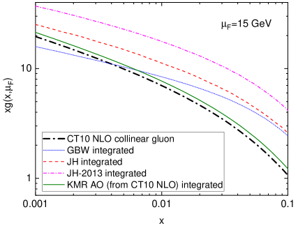
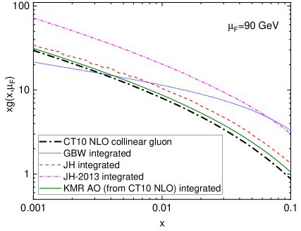
Figure 5: The “collinear integral” (23) computed for the four indicated unintegrated gluon distributions and two factorization scales $\mu_{F}$ as a function of $x$, compared to the collinear gluon distribution CT10 at the NLO.

IV Comparison to data

IV.1 Isolation of $\gamma$

In order to perform the comparison of our numerical results with the LHC data, we need to perform photon isolation from jets in similar manner as it was done by the ATLAS and CMS experiments. To this end, we implement the Frixione cone cut at the parton level Frixione:1998jh . For the final state $q\bar{q}\gamma$, we define the distances $R_{i}$ between the outgoing quarks, labeled by $i=3,4$, and the photon:

$$R_{i}=\sqrt{(\phi_{i}-\phi_{\gamma})^{2}+(y_{i}-y_{\gamma})^{2}}\,,$$ (24)

where $\phi_{i}$ are parton azimuthal angles and $y_{i}$ are their rapidity. We take $R_{0}=0.4$. The Frixione cone isolation procedure leads then to the following conditions which have to be satisfied by the kinematic configuration:

• if $R_{3}<R_{4}<R_{0}$ then

  $$p_{3T}+p_{4T}<q_{T}\frac{1-\cos R_{4}}{1-\cos R_{0}}\,~{}~{}~{}~{}~{}~{}{\rm and}~{}~{}~{}~{}~{}~{}p_{3T}<q_{T}\frac{1-\cos R_{3}}{1-\cos R_{0}}\,,~{}~{}~{}~{}~{}~{}~{}~{}$$ (25)

• if $R_{3}<R_{0}<R_{4}$ then

  $$p_{3T}<q_{T}\frac{1-\cos R_{3}}{1-\cos R_{0}}\,,$$ (26)

• no constrains when $R_{0}<R_{3}<R_{4}$,

• if $R_{4}>R_{3}$ then conditions (25) and (26) are applied with the indices $3\leftrightarrow 4$,

• for simpler partonic final states, $q\gamma$ and $\bar{q}\gamma$, only condition (26) is imposed.

IV.2 LHC data sets

In the comparison, we focus on the available sets of data that probe the smallest values of gluon $x$ variable. Hence we choose the following measurements of the prompt photon production from the ATLAS and CMS experiments:

• ATLAS data at $\sqrt{S}=7~{}{\rm TeV}$ with $15~{}{\rm GeV}<q_{T}<100~{}{\rm GeV}$ (ATLAS$@7{\rm TeV}$) Aad:2010sp ,

• CMS data at $\sqrt{S}=7~{}{\rm TeV}$ with $25~{}{\rm GeV}<q_{T}<400~{}{\rm GeV}$ (CMS$@7{\rm TeV}$) Chatrchyan:2011ue ,

• ATLAS data at $\sqrt{S}=8~{}{\rm TeV}$ with $25~{}{\rm GeV}<q_{T}<1500~{}{\rm GeV}$ (ATLAS$@8{\rm TeV}$) Aad:2016xcr ,

where $q_{T}$ is the photon transverse momentum. In these experiments the cross sections were measured as a function of $q_{T}$ in several rapidity intervals. In the following figures, the experimental data are compared to theoretical predictions obtained within the $k_{T}$-factorization formalism in the two schemes described in the previous sections: the $qg^{*}$ scheme based on the $qg^{*}\to q\gamma$ and $\bar{q}g^{*}\to\bar{q}\gamma$ partonic channels, and the $g^{*}g^{*}$ scheme based on a combination of the $q_{\mathrm{val}}g^{*}\to q\gamma$ and $g^{*}g^{*}\to q\bar{q}\gamma$ channels. For each theoretical scheme, we display the results obtained with the three unintegrated gluon distributions: KMR-AO, JH and GBW.

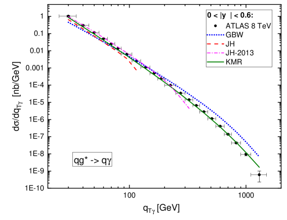
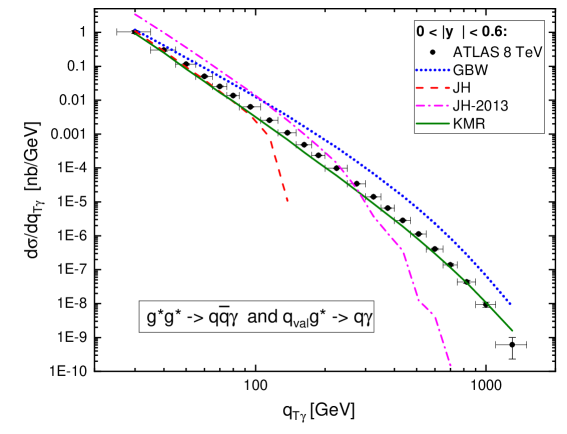
Figure 6: Prompt photon production cross section computed in the $qg^{*}$ (top) and $g^{*}g^{*}$ (bottom) schemes with the indicated unintegrated gluon distributions, compared to the ATLAS$@8{\rm TeV}$ data Aad:2016xcr for the central rapidity bin.

IV.3 Comparison to data

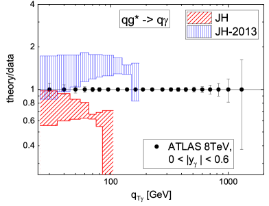
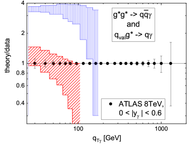
Figure 7: Theory to experiment ratios for the prompt photon production at ATLAS@8 TeV obtained from the JH and JH-2013 unintegrated gluon distributions within the $qg^{*}$ (right) and $g^{*}g^{*}$ (left) schemes for the central rapidity bin.

In Fig. 6, we show the theory curves against the ATLAS$@8{\rm TeV}$ data for the central rapidity, $|y|<0.6$, in the log-log scale. This is the way the experimental results are usually presented. In the upper plot, the predictions are obtained in the $qg^{*}$ scheme while in the lower plot the predictions are computed in the $g^{*}g^{*}$ scheme. Clearly, the $qg^{*}$ scheme with the KMR-AO gluon distribution gives the best description of the data. The same gluon distribution used in the $g^{*}g^{*}$ scheme leads to a reasonable description of the data, but the cross section is somewhat underestimated for intermediate values of $q_{T}$. The cross sections obtained with the JH and KMR-AO distributions are very close to each other for $q_{T}<100~{}{\rm GeV}$, where the JH parametrization may be applied.

The new JH-2013 parametrization allows to extend the JH results up to $k_{T}\simeq 300~{}{\rm GeV}$. However, the agreement with the data for $k_{T}<100~{}{\rm GeV}$ becomes much worse in the $g^{*}g^{*}$ scheme. The predictions obtained with the GBW gluon are close to the data at lower $q_{T}$, but lead to too flat $q_{T}$-dependence. Clearly, this is due to too flat $x$-dependence of the GBW gluon, discussed in more detail in the previous section. Based on Fig. 6, one concludes that the best description of the prompt photon data from the LHC in the full range of the measured photon transverse momentum is obtained for the KMR-AO gluon distribution in both the $qg^{*}$ and $g^{*}g^{*}$ schemes.

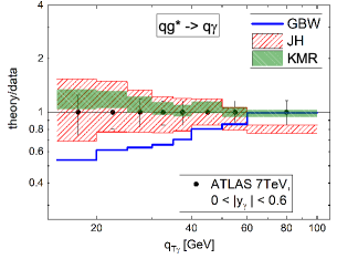
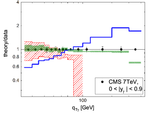
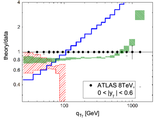
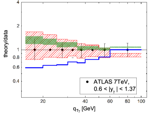
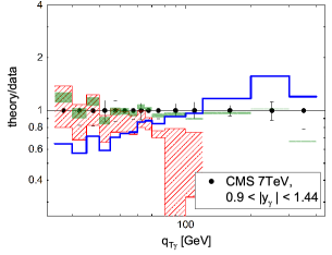
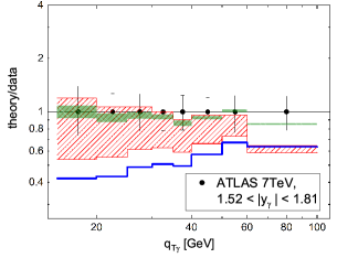
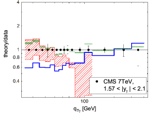
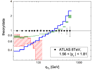
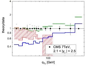
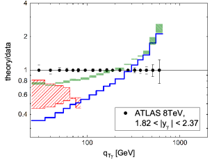
Figure 8: Theory to experiment ratios for the prompt photon production within the $qg^{*}$ scheme for the ATLAS$@7{\rm TeV}$ Aad:2010sp (left column), CMS$@7{\rm TeV}$ Chatrchyan:2011ue (central column) and ATLAS$@8{\rm TeV}$ Aad:2016xcr (right column) data and the KMR-AO (green shaded bands), JH (red hatched bands) and GBW (blue curves) unintegrated gluon distributions. The theory uncertainties are due to the variation of the factorization scale $\mu_{F}=\mu_{R}$ between $q_{T}/2$ and $2q_{T}$.

In order to perform more detailed studies of the description quality, we change the way the data and theoretical results are presented. Namely, in Figs. 7, 8 and 9 we display the ratios of the theoretical results to the experimental data. For the sake of the optimal comparison, the theoretical result are integrated over the bins used in the experiments. The theoretical uncertainties are due to the variation of the factorization scales, $\mu_{F}=\mu_{R}$, between $q_{T}/2$ and $2q_{T}$.

In Fig. 7, using central bin of the ATLAS$@8{\rm TeV}$ data, we show the typical result for the comparison of the data with the predictions given by the JH and JH-2013 gluon distributions. We see that the new JH-2013 distribution significantly overestimates the data for $q_{T}<100~{}{\rm GeV}$. This could be attributed to a much higher the JH-2013 gluon distribution than the JH one for the gluon $k_{T}<1~{}{\rm GeV}$, see Fig. 4. In the forthcoming analyses we will show only the JH predictions.

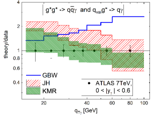
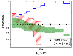
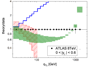
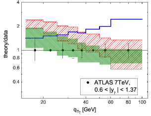
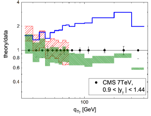
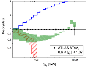
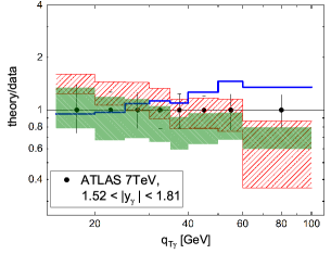
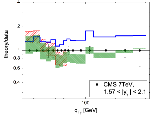
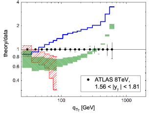
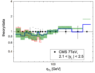
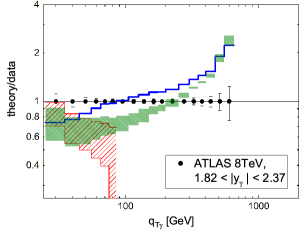
Figure 9: Theory to experiment ratios for the prompt photon production within the $g^{*}g^{*}$ scheme for the ATLAS$@7{\rm TeV}$ Aad:2010sp (left column), CMS$@7{\rm TeV}$ Chatrchyan:2011ue (central column) and ATLAS$@8{\rm TeV}$ Aad:2016xcr (right column) data and the KMR-AO (green shaded bands), JH (red hatched bands) and GBW (blue curves) unintegrated gluon distributions. The theory uncertainties are due to the variation of the factorization scale $\mu_{F}=\mu_{R}$ between $q_{T}/2$ and $2q_{T}$.

The theory to data ratios obtained within the $qg^{*}$ scheme are shown in Fig. 8 for the three considered LHC data sets. The absolute value of the photon rapidities $|y|$ grows from the top row down. Clearly, the best overall description of the data is found with the KMR-AO gluon (green shaded bands). It is seen at best for the data set with the smallest errors, that is the ATLAS$@8{\rm TeV}$ data (right column). For most bins, these theoretical results are close to the data, with relative differences smaller than 20%. Given the fact that the leading order $k_{T}$-factorization approach is used, this is a very good accuracy. Somewhat larger deviations are found only for larger values of $|y|$ and $q_{T}>500$ GeV. In this region, however, the $k_{T}$-factorization approach is less accurate since the contributions from relatively large values of the gluon $x$ are becoming important. The scale uncertainty of these results is very small and does not allow to overlap with the data. The description of the CMS$@7{\rm TeV}$ data with $q_{T}<400$ GeV (middle column) with the KMR-AO gluon is also very good for all rapidities. The predictions for ATLAS$@7{\rm TeV}$ (left column) are above the central data points, but stays consistent with the data within the experimental errors, somewhat larger in this measurement.

The data description in Fig. 8 with the JH gluon (red hatched bands) is reasonable, but the application of this gluon is limited to $q_{T}<100$ GeV. The results calculated with JH are somewhat below the KMR-AO results and more away from the CMS$@7{\rm TeV}$ and ATLAS$@8{\rm TeV}$ data. This is interesting in the context of Fig. 5, where one sees a larger integrated gluon from JH than from KMR-AO distributions. This suggests that the lower prompt photon production cross sections from the JH distribution are due to the cut-off of larger transverse momenta, $k_{T}>\mu_{F}$, that is not present in the KMR-AO case, see Fig. 4. This shows that the prompt photon data are sensitive to the shape of the transverse momentum gluon distribution, and that the longer $k_{T}$-tail of the KMR-AO distribution is preferred by the data.

We also see that the uncertainty of the cross section due to scale variation is much larger for JH than for KMR-AO. The gluon from the GBW model does not reproduce well the $q_{T}$-dependence of the data. The predictions are significantly below the data at the lower limits of $q_{T}$ and much above data at very large $q_{T}$. One has to remember, however, that in our study the GBW model is used far outside the range of very small $x$ values and moderate scales, where it was fitted and should work well. The deviations from the data reflect the tendency visible already in the integrated GBW gluon, see Fig. 5 and the corresponding discussion of its content.

Let us move now to the other approach, the $g^{*}g^{*}$ scheme, which results are shown in Fig. 9. Here the cross sections are obtained by adding the $g^{*}g^{*}\to q\bar{q}\gamma$ and $q_{\mathrm{val}}\,g^{*}\to q\gamma$ contributions. Due to different dependencies on $x$ of the valence quark and gluon distributions, the $g^{*}g^{*}\to q\bar{q}\gamma$ is dominant at lower $q_{T}$ while $q_{\mathrm{val}}\,g^{*}\to q\gamma$ takes over at larger $q_{T}$. In the region where the gluon $x$ is small or moderate, i.e. for $q_{T}<50~{}{\rm GeV}$, the $g^{*}g^{*}$ scheme gives a rather good description of all the data sets with the KMR-AO gluon. The scale uncertainty is significantly larger than it was for the $qg^{*}$ scheme. This approach, however, is consistently less successful for $q_{T}>50$ GeV. The biggest deviation occurs in the region of $q_{T}\sim~{}300-500~{}{\rm GeV}$, where the theory to experiment ratio is at the level of $0.6-0.7$. For larger $q_{T}$, the theory results become dominated by the $q_{\mathrm{val}}\,g^{*}\to q\gamma$ channel, and the results approach the results of the $qg^{*}$ scheme, see Fig. 10. Within its limits of applicability, the JH gluon gives rather similar results to the KMR-AO gluon, hence well consistent with the data. The approach based on the GBW gluon experiences strengthened problems due to inaccuracy of the used extrapolation beyond $x>0.01$ and too mild scale dependence since the gluon distribution enters the hadronic cross sections twice in the $g^{*}g^{*}$ scheme.

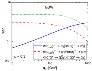
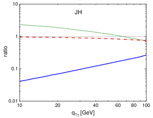
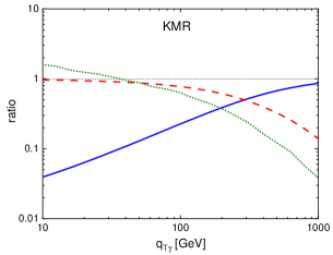
Figure 10: Decomposition of the prompt photon production cross section into partonic channels in $qg^{*}$ and $g^{*}g^{*}$ schemes. Plotted ratios of the partonic cross sections: $\sigma(q_{\mathrm{val}}g^{*})/\sigma(qg^{*})$, $\sigma(q_{\mathrm{sea}}g^{*})/\sigma(qg^{*})$, and $\sigma(g^{*}g^{*})/\sigma(qg^{*})$.

There is an interesting message coming from the comparison of the results in the $qg^{*}$ anf $g^{*}g^{*}$ schemes. On the diagrammatic level, the $g^{*}g^{*}$ contribution incorporates the $q_{\mathrm{sea}}\,g^{*}$ contribution, where the sea quark is produced in the last splitting. Therefore, one expects that the $g^{*}g^{*}$ scheme should lead to results that are close to the $qg^{*}$ scheme. This is, however, not confirmed by the data at larger $q_{T}$. In order to provide more insight into this problem, in Fig. 10 we show the partonic components of the cross sections in both the schemes. We plot the ratios: $\sigma(q_{\mathrm{val}}g^{*})/\sigma(qg^{*})$, $\sigma(q_{\mathrm{sea}}g^{*})/\sigma(qg^{*})$ and $\sigma(g^{*}g^{*})/\sigma(qg^{*})$, where the reference cross section $\sigma(qg^{*})=\sigma(q_{\mathrm{sea}}g^{*})+\sigma(q_{\mathrm{val}}g^{*})$ is obtained in the $qg^{*}$ scheme. Note that $\sigma(q_{\mathrm{val}}g^{*})$ is the same in both schemes.

Clearly, at lower $q_{T}$, that is for smaller values of the parton $x$, the $q_{\mathrm{sea}}\,g^{*}$ or $g^{*}g^{*}$ contributions strongly dominate over the $q_{\mathrm{val}}\,g^{*}$ channel. For $q_{T}\sim 200-600~{}{\rm GeV}$, depending on the scheme, the $q_{\mathrm{val}}\,g^{*}$ channel is leading. Interestingly enough, both for the KMR-AO and JH gluons, the $g^{*}g^{*}$ channel is larger at the lowest $q_{T}=10~{}{\rm GeV}$, but it decreases faster with $q_{T}$ than the $q_{\mathrm{sea}}\,g^{*}$ channel, and at $q_{T}\sim 1000~{}{\rm GeV}$ the difference is already very pronounced. At this stage, we do not have good understanding of this behavior. One could attempt to connect this deviation to going out of the small $x$ domain, but this simple explanation is undermined by the fact that the results obtained in the $qg^{*}$ scheme stay close to data even at $q_{T}\sim 1000~{}$GeV, where the gluon $x$ is not small. Hence we consider this problem to be an interesting theoretical puzzle that calls for explanation.

V Conclusions

In this paper, we have analyzed the prompt photon hadroproduction at the LHC using the $k_{T}$-factorization approach with the $qg^{*}\to q\gamma$ and $g^{*}g^{*}\to q\bar{q}\gamma$ partonic channels.The data from the ATLAS and CMS collaboration were considered, obtained at $\sqrt{S}=7$ TeV and $\sqrt{S}=8$ TeV with the range of the photon transverse momentum from $15~{}{\rm GeV}$ to $1500~{}{\rm GeV}$ in several rapidity bins of the photon. The unintegrated, transverse momentum dependent gluon distributions of different origin were probed: from the integral KMR procedure with angular ordering (KMR-AO), the Jung–Hansson distribution (JH) obtained from the CCFM equation as well as the Jung-Hautmann newer version JH-2013 and the gluon distribution from the GBW saturation model extended to large values of $x$.

With the $qg^{*}$ partonic channel and the KMR-AO gluon distribution, the best overall description of the data was obtained with typical accuracy of $10-20\%$. The results obtained with the JH gluon were found to be slightly less accurate in the region of their applicability with $q_{T}<100~{}{\rm GeV}$. The JH-2013 results significantly overshoot the data. The GBW gluon does not provide satisfactory description beyond this region and for central values of the photon rapidity, which shows the expected region of its validity due to small-$x$ nature of this distribution.

We point out that our findings indicate that the precision prompt photon data allow for constraining the transverse momentum distribution of the gluons in the proton. At larger photon rapidities, the JH description of the data deteriorates for increasing photon transverse momentum $q_{T}$, underestimating the data while the KMR-AO description stays close to the data. This effect may be traced back to a much steeper decrease of the JH distribution than the KMR-AO one for gluon transverse momenta $k_{T}$ larger than the factorization scale $\mu_{F}$.

The description obtained with the $g^{*}g^{*}$ channel was shown to provide a good description of the data at lower photon transverse momentum $q_{T}$, where also the values of the partons’ $x$ are lower. At larger $q_{T}$, however, the data are significantly underestimated in this approach. We find this result rather puzzling as the $g^{*}g^{*}$ channel should partially include the NLO effects besides the sea quark contributions to the $qg^{*}$ channel from the last splitting, which is the main contribution to the total $qg^{*}$ channel. This puzzle calls for a complete NLO analysis of the prompt photon hadroproduction in the $k_{T}$-factorization framework.

References

- (1) L. Gribov, E. Levin and M. Ryskin, Phys. Rept. 100, 1 (1983).
- (2) S. Catani, M. Ciafaloni and F. Hautmann, Phys. Lett. B 242, 97 (1990).
- (3) S. Catani, M. Ciafaloni and F. Hautmann, Nucl. Phys. B 366, 135 (1991).
- (4) M. Deak and F. Schwennsen, JHEP 09, 035 (2008), [0805.3763].
- (5) L. Motyka, M. Sadzikowski and T. Stebel, Phys. Rev. D 95, 114025 (2017), [1609.04300].
- (6) V. S. Fadin, E. A. Kuraev and L. N. Lipatov, Phys. Lett. B60, 50 (1975).
- (7) E. A. Kuraev, L. N. Lipatov and V. S. Fadin, Sov. Phys. JETP 45, 199 (1977), [Zh. Eksp. Teor. Fiz.72,377(1977)].
- (8) I. I. Balitsky and L. N. Lipatov, Sov. J. Nucl. Phys. 28, 822 (1978), [Yad. Fiz.28,1597(1978)].
- (9) M. Ciafaloni, Nucl. Phys. B296, 49 (1988).
- (10) S. Catani, F. Fiorani and G. Marchesini, Nucl. Phys. B336, 18 (1990).
- (11) S. Catani, F. Fiorani and G. Marchesini, Phys. Lett. B234, 339 (1990).
- (12) G. Marchesini, Nucl. Phys. B445, 49 (1995), [hep-ph/9412327].
- (13) B. Kopeliovich, Soft component of hard reactions and nuclear shadowing, in 23rd International Workshop on Gross Properties of Nuclei and Nuclear Excitations: Dynamical Properties of Hadrons in Nuclear Matter (Hirschegg ’95), pp. 102–112, 1995, [hep-ph/9609385].
- (14) B. Z. Kopeliovich, A. V. Tarasov and A. Schafer, Phys. Rev. C 59, 1609 (1999), [hep-ph/9808378].
- (15) J. Jalilian-Marian and A. H. Rezaeian, Phys. Rev. D 86, 034016 (2012), [1204.1319].
- (16) S. Benic and K. Fukushima, Nucl. Phys. A 958, 1 (2017), [1602.01989].
- (17) S. Benic, K. Fukushima, O. Garcia-Montero and R. Venugopalan, JHEP 01, 115 (2017), [1609.09424].
- (18) S. Benić, K. Fukushima, O. Garcia-Montero and R. Venugopalan, Phys. Lett. B 791, 11 (2019), [1807.03806].
- (19) B. Ducloué, T. Lappi and H. Mäntysaari, Phys. Rev. D 97, 054023 (2018), [1710.02206].
- (20) S. Baranov, A. Lipatov and N. Zotov, Phys. Rev. D 77, 074024 (2008), [0708.3560].
- (21) S. Baranov, A. Lipatov and N. Zotov, J. Phys. G 36, 125008 (2009), [0811.2575].
- (22) A. Lipatov, M. Malyshev and N. Zotov, Phys. Lett. B 699, 93 (2011), [1102.1134].
- (23) A. Lipatov and M. Malyshev, Phys. Rev. D 94, 034020 (2016), [1606.02696].
- (24) B. Kniehl, V. Saleev, A. Shipilova and E. Yatsenko, Phys. Rev. D 84, 074017 (2011), [1107.1462].
- (25) G. Sampaio dos Santos, G. Gil da Silveira and M. Machado, Eur. Phys. J. C 80, 812 (2020), [2004.02686].
- (26) V. P. Goncalves, Y. Lima, R. Pasechnik and M. Šumbera, Phys. Rev. D 101, 094019 (2020), [2003.02555].
- (27) S. Brodsky, A. Hebecker and E. Quack, Phys. Rev. D 55, 2584 (1997), [hep-ph/9609384].
- (28) L. D. McLerran and R. Venugopalan, Phys. Rev. D 49, 2233 (1994), [hep-ph/9309289].
- (29) L. D. McLerran and R. Venugopalan, Phys. Rev. D 49, 3352 (1994), [hep-ph/9311205].
- (30) L. D. McLerran and R. Venugopalan, Phys. Rev. D 50, 2225 (1994), [hep-ph/9402335].
- (31) S. Frixione, Phys. Lett. B 429, 369 (1998), [hep-ph/9801442].
- (32) ATLAS, G. Aad et al., Phys. Rev. D 83, 052005 (2011), [1012.4389].
- (33) CMS, S. Chatrchyan et al., Phys. Rev. D 84, 052011 (2011), [1108.2044].
- (34) ATLAS, G. Aad et al., JHEP 08, 005 (2016), [1605.03495].
- (35) K. J. Golec-Biernat and M. Wusthoff, Phys. Rev. D 59, 014017 (1998), [hep-ph/9807513].
- (36) K. Golec-Biernat and S. Sapeta, JHEP 03, 102 (2018), [1711.11360].
- (37) X. Chen, T. Gehrmann, N. Glover, M. Höfer and A. Huss, JHEP 04, 166 (2020), [1904.01044].
- (38) L. Motyka, M. Sadzikowski and T. Stebel, JHEP 05, 087 (2015), [1412.4675].
- (39) D. Brzeminski, L. Motyka, M. Sadzikowski and T. Stebel, JHEP 01, 005 (2017), [1611.04449].
- (40) J. C. Collins and R. Ellis, Nucl. Phys. B 360, 3 (1991).
- (41) J. Vermaseren, math-ph/0010025.
- (42) I. Balitsky, Nucl. Phys. B 463, 99 (1996), [hep-ph/9509348].
- (43) Y. V. Kovchegov, Phys. Rev. D 60, 034008 (1999), [hep-ph/9901281].
- (44) Y. V. Kovchegov, Phys. Rev. D 61, 074018 (2000), [hep-ph/9905214].
- (45) M. A. Kimber, A. D. Martin and M. G. Ryskin, Eur. Phys. J. C12, 655 (2000), [hep-ph/9911379].
- (46) M. A. Kimber, A. D. Martin and M. G. Ryskin, Phys. Rev. D63, 114027 (2001), [hep-ph/0101348].
- (47) M. Hansson and H. Jung, Status of CCFM: Unintegrated gluon densities, in 11th International Workshop on Deep Inelastic Scattering (DIS 2003), pp. 488–492, 2003, [hep-ph/0309009].
- (48) K. Golec-Biernat and A. M. Stasto, Phys. Lett. B 781, 633 (2018), [1803.06246].
- (49) H.-L. Lai et al., Phys. Rev. D 82, 074024 (2010), [1007.2241].
- (50) F. Hautmann, H. Jung, A. Lelek, V. Radescu and R. Zlebcik, JHEP 01, 070 (2018), [1708.03279].
- (51) K. Golec-Biernat and T. Stebel, Eur. Phys. J. C 80, 455 (2020), [1911.10103].
- (52) F. Hautmann and H. Jung, Nucl. Phys. B 883, 1 (2014), [1312.7875].