Study of the Kondo and high temperature limits of the slave boson and X-boson methods

Abstract

In this paper we study the periodic Anderson model, employing both the slave-boson and the X-boson approaches in the mean field approximation. We investigate the breakdown of the slave boson at intermediate temperatures when the total occupation number of particles $N_{t}=N_{f}+N_{c}$ is keep constant, where $N_{f}$ and $N_{c}$ are respectively the occupation numbers of the localized and conduction electrons, and we show that the high temperature limit of the slave boson is $N_{f}=N_{c}=N_{t}/2$. We also compare the results of the two approaches in the Kondo limit and we show that at low temperatures the X-boson exhibits a phase transition, from the Kondo heavy Fermion (K-HF) regime to a local moment magnetic regime (LMM).

, ,

1 Introduction

The PAM is one of several models of correlated electrons that has been very useful to describe important physical systems, like transition metals and heavy fermions (HF). Indeed, heavy fermion materials present a great variety of ground states: antiferromagnetic (UAgCu₄, UCu₇), superconducting (CeCu₂Si₂, UPt₃), Fermi liquids (CeCu₆, CeAl₃) and Kondo insulators (Ce₃B$i_{4}$P$t_{3}$, YbB₁₂) [1, 2, 3, 4]. A uniform Curie-like magnetic susceptibility at high temperature, a common feature of these compounds, is related to the fact that they contain elements with incomplete $f$-shells, like $Ce$ and $U$. As the temperature decreases to a certain range, the system presents a temperature independent uniform susceptibility (Pauli susceptibility), signaling the quenching of the localized magnetic moments of the $f$-states, and resembling the behavior of the single-impurity Kondo problem [5]. The consistent description of the overall properties of the heavy fermions is achieved by the competition between the Kondo effect, dealing with the quenching of the localized magnetic moments, and the Ruderman, Kittel, Kasuya, Yosida (RKKY) interaction, which favors the appearance of a magnetic ground state. The basic Hamiltonian that describes the physics of the HF system should then be a regular lattice of $f$-moments interacting with an electron gas, and this is the basis of the periodic Anderson model (PAM), that usually neglects the orbital degeneracy of the f-electrons, treating them as if they were s-electrons. This interaction mediates, in higher order, the RKKY magnetic interaction between the f-electrons.

This work compares the results of the mean field slave boson theory (MFSBT) with those of the mean field X-boson theory (MFXBT) in the Kondo and in the high temperature limits of the PAM [6, 7, 8, 9, 10], taking a constant number of total electrons per site $N_{t}$. This paper is organized as follows: in the next section we make a brief revision of the MFSBT and we calculate $z$, the average number of slave-bosons per site in the system. In section 3 these results are compared with those obtained by the X-boson method. In section 5 we calculate the density of states and the entropy of the system, and compare the numerical results of the two methods. In section 6 we review the main results of the present work. In Appendix A we calculate an analytical expression for the temperature at which $z\rightarrow 0$ in the weak-coupling limit, and in Appendix B we calculate the MFSBT and MFXBT occupation of $f$-electrons and $c$-electrons in the high temperature limit.

2 The slave-boson method

In this paper we discuss the periodic Anderson model (PAM) in the limit of infinite correlation $U\rightarrow\infty$, described by the Hamiltonian

$$H=\sum_{\mathbf{k},\sigma}E_{\mathbf{k},\sigma}c_{\mathbf{k},\sigma}^{\dagger}c_{\mathbf{k},\sigma}+\sum_{\mathbf{j},\sigma}{E}_{f,\mathbf{j,\sigma}}X_{\mathbf{j},\sigma\sigma}+$$

$$\frac{1}{\sqrt{\mathcal{N}_{s}}}\sum_{\mathbf{j},\mathbf{k},\sigma}\left(v_{\mathbf{k}}e^{i\mathbf{k}.\mathbf{r}_{j}}X_{\mathbf{j},0\sigma}^{{\dagger}}c_{\mathbf{k},\sigma}+v_{\mathbf{k}}^{\ast}e_{j}^{-i\mathbf{k}.\mathbf{r}}c_{\mathbf{k},\sigma}^{\dagger}X_{\mathbf{j},0\sigma}\right)\,.$$ (1)

The first term is the kinetic energy of the conduction electrons ($c$-electrons), described by the usual Fermi operators, while the second term is the energy of the localized electrons ($f$-electrons). The last term represents the hybridization between the $c$-electrons and the $f$-electrons and we neglect the $f$-$f$ hopping.

An auxiliary boson field is introduced in the slave-boson method [6], and the Hubbard operators at site $\mathbf{j}$ are rewritten as a product of ordinary boson and fermion operators $X_{\mathbf{j},0\sigma}^{{\dagger}}\rightarrow f_{\mathbf{j},\sigma}^{\dagger}b_{\mathbf{j}}\ ,X_{\mathbf{j},0\sigma}\rightarrow b_{\mathbf{j}}^{\dagger}f_{\mathbf{j},\sigma}$. To eliminate spurious states, only those that preserve the identity

$$b_{\mathbf{j}}^{\dagger}b_{\mathbf{j}}+\sum_{\sigma}f_{\mathbf{j}\sigma}^{\dagger}f_{\mathbf{j}\sigma}=I_{\mathbf{j}},$$ (2)

are considered, and it then follows that $X_{\mathbf{j},00}\rightarrow b_{\mathbf{j}}^{\dagger}b_{\mathbf{j}}\$, and $X_{\mathbf{j},\sigma\sigma}\rightarrow f_{\mathbf{j},\sigma}^{\dagger}f_{\mathbf{j},\sigma}$. At a later stage Lagrange’s method is employed to minimize the thermodynamic potential with the identity 2 as a constrain, and one then has to add the operator $Q_{\mathbf{j}}\equiv\lambda_{\mathbf{j}}\left(b_{\mathbf{j}}^{\dagger}b_{\mathbf{j}}+\sum_{\sigma}f_{\mathbf{j},\sigma}^{\dagger}f_{\mathbf{j},\sigma}-I_{\mathbf{j}}\right)$ to the model Hamiltonian, where $\lambda_{\mathbf{j}}$ are the Lagrange multipliers. To use the grand canonical ensemble, we also have to subtract from the Hamiltonian the operator $\mu\left\{\sum_{\mathbf{j},\sigma}f_{\mathbf{j},\sigma}^{\dagger}f_{\mathbf{j},\sigma}+\sum_{\mathbf{k},\sigma}c_{\mathbf{k},\sigma}^{\dagger}c_{\mathbf{k},\sigma}\right\}$ where $\mu$ is the chemical potential of the electrons. The MFSBT is obtained when we neglect the fluctuations of the boson operators by replacing $b_{\mathbf{j}}$ and $b_{\mathbf{j}}^{\dagger}$ by their averages. We assume that the local energies ${E}_{f,\mathbf{j},\sigma}\rightarrow{E}_{f}$ and $E_{\mathbf{k},\sigma}\rightarrow E_{\mathbf{k}}$ are site independent and that the hybridization constant is equal to $V$. Considering translational invariance we can write $\left\langle b_{\mathbf{j}}^{\dagger}\right\rangle=\left\langle b_{\mathbf{j}}\right\rangle=\sqrt{z}$, we then obtain the transformed Hamiltonian

$$H_{\mbox{\scriptsize{S-B}}}=\sum_{\mathbf{k},\sigma}{\epsilon}_{\mathbf{k}}\ c_{\mathbf{k},\sigma}^{\dagger}c_{\mathbf{k},\sigma}+\sum_{\mathbf{k},\sigma}\tilde{{E}}_{f}\ f_{\mathbf{k},\sigma}^{\dagger}f_{\mathbf{k},\sigma}+$$

$$\sum_{\mathbf{k},\sigma}\tilde{V}\ (c_{\mathbf{{k},\sigma}}^{\dagger}\ f_{\mathbf{k},\sigma}+c_{\mathbf{k},\sigma}\ f_{\mathbf{k},\sigma}^{\dagger})+\mathcal{N}_{s}\lambda\left(z-1\right)\,,$$ (3)

where ${\epsilon}_{\mathbf{k}}={E}_{\mathbf{k}}-\mu$ and the localized electrons acquire a renormalized energy $\tilde{{E}}_{f}=\epsilon_{f}+\lambda$ with $\epsilon_{f}=E_{f}-\mu$, and this Hamiltonian describes a simple uncorrelated Anderson lattice with renormalized $\tilde{V}\rightarrow\sqrt{z}\ V$ and $\tilde{{E}}_{f}$. This model has the following Green’s functions (GF) [11]:

$${\ \mathcal{G}}_{\sigma}^{f}(\mathbf{k},\omega)\equiv\ll f_{\mathbf{k},\sigma};f_{\mathbf{k},\sigma}^{\dagger}\gg_{\omega}\ =$$

$$\frac{-\left(i\omega-\epsilon_{\mathbf{k}}\right)}{\left(i\omega-\tilde{E_{f}}\right)\left(i\omega-\epsilon_{\mathbf{k}}\right)-|\tilde{V}|^{2}},$$ (4)

with similar expressions for the others Green’s functions ${\mathcal{G}}_{\sigma}^{cf}(\mathbf{k},\omega)=\ll c_{\mathbf{k},\sigma};X_{\mathbf{k},0\sigma}^{\dagger}\gg_{\omega}$ and ${\mathcal{G}}_{\sigma}^{c}(\mathbf{k},\omega)=\ll c_{\mathbf{k},\sigma};c_{\mathbf{k},0\sigma}^{\dagger}\gg_{\omega},$ all of them having poles at $\omega_{\pm}$:

$$\omega_{\pm}=\frac{1}{2}\left(\epsilon_{\mathbf{k}}+\tilde{E_{f}}\pm\sqrt{(\epsilon_{\mathbf{k}}-\tilde{{E}}_{f})^{2}+4\tilde{V}^{2}}\right)\,.$$ (5)

The occupations per site $N_{f}\equiv\left(1/\mathcal{N}_{s}\right)\sum_{\sigma,\mathbf{k}}\langle f_{\mathbf{k,\sigma}}^{\dagger}f_{\mathbf{k}\sigma}\rangle$, and $N_{c}\equiv\left(1/\mathcal{N}_{s}\right)\sum_{\sigma,\mathbf{k}}\langle c_{\mathbf{k},\sigma}^{\dagger}c_{\mathbf{k},\sigma}\rangle$, as well as the average $N_{cf}\equiv\left(1/\mathcal{N}_{s}\right)\sum_{\sigma,\mathbf{k}}\langle c_{\mathbf{k},\sigma}f_{\mathbf{k},\sigma}^{\dagger}\rangle$, can be obtained from these Green’s functions.

For a certain region of the parameter space there is a  “condensation temperature” $T_{\mbox{\scriptsize{cond}}}$ where $z\rightarrow 0$ . This $T_{\mbox{\scriptsize{cond}}}$ was calculated in the Appendix A in the weak-coupling limit (cf. (16)), and when we employ the simple density of states

$$\rho(E_{\mathbf{k}})=\left\{\begin{array}[c]{l}(2D)^{-1},\mbox{ for }-D\leq E_{\mathbf{k}}\leq D\\ 0\qquad\mbox{\ ,\ \ otherwise }\end{array}\right.$$ (6)

it can be re-expressed as

$$k_{B}T_{\mbox{\scriptsize{cond}}}\sim\left(D-\mu\right)\exp\left\{-1/(N_{\sigma}\rho_{c}(\mu)J_{K})\right\}\,.$$ (7)

In this equation $J_{K}$ is the Kondo coupling obtained via the Schrieffer-Wolff transformation [19], $\rho_{c}(\mu)$ is the density of states of the $c$-electrons at the chemical potential, $D-\mu$ can be interpreted as a cut-off energy measured from the chemical potential and $N_{\sigma}$ is the number of spin components per state $\mathbf{k}$. This is the well-known expression for the single-impurity Kondo temperature [3] and $T_{\mbox{\scriptsize{cond}}}$ is often identified to be the actual Kondo temperature of the lattice in the mean-field slave-boson theory. However, as shall be discussed below, such identification is not appropriate for all  the values of the total number of electrons $N_{t}=N_{f}+N_{c}$. A drawback of the MFSBT is that the formalism present a discontinuity at $T=T_{\mbox{\scriptsize{cond}}}$ [7, 8, 12], which defines a spurious second-order phase transition that is not observed experimentally. Indeed, at the condensation temperature we have $N_{f}=1$, so that $z=1-N_{f}=0$ and $\tilde{V}\equiv\sqrt{z}\ V=0$, decoupling the two bands of the model Hamiltonian.

To analyze this behavior of the MFSBT, we calculate $z$ as a function of the temperature $T$ for several values of $N_{t}$. In our numerical calculations we employ $E_{f}=$ $-0.15D$ as the bare localized $f$-energy and $V=0.20D$ as the hybridization respectively, and use the density of states given by (6).

 

Figure 1: The temperature dependence of slave-boson parameter $z$ for several $N_{t}$. $E_{f}=-0.15D$ and the hybridization parameter $V$ is $V=0.20D$. All the energies are given in units of $D$.

There is a belief in literature that, for the lattice case, the collapse of the quasi-particles bands in the MFSBT, occurs only at very high temperatures, in contrast with the impurity case where this breakdown occurs at the condensation temperature $T_{cond}$ (see reference [3] - pg. $343$). But the results summarized in figure 1, shows that for the lattice case, the MFSBT present a more complex behavior. We identify four distinct regimes for $z$ as a function of $T$. (i) For $N_{t}=1.8$, the parameter $z$ is positive for all $T$, and the system never reaches a temperature $T=T_{\mbox{\scriptsize{cond}}}$. (ii) For $N_{t}=1.95$, $z$ crosses the horizontal axis in two points, defining two condensation temperatures and the reason for this behavior is that $N_{f}=N_{c}$ in the high temperature limit (cf. the Appendix B), so that $z=1-N_{f}$ becomes again positive in this limit. (iii) For $N_{t}\gtrsim 2$ ($N_{t}=2.03$ in the figure), $z$ is negative for all $T>T_{\mbox{\scriptsize{cond}}}$ and positive otherwise. (iv) Finally, in the high occupations regime ($N_{t}=2.1$ in the figure), $z$ is negative for all temperatures. However, note that the system never reaches $T_{\mbox{\scriptsize{cond}}}$ for $N_{t}\lesssim 1.9$, so that $T_{\mbox{\scriptsize{cond}}}$ cannot be identified to be the Kondo temperature of the lattice. The $T=T_{\mbox{\scriptsize{cond}}}$ is defined in a unique way in the impurity case, because all the calculations are performed with a constant chemical potential $\mu$, but in the lattice case it is the total number of particles that should be kept constant, and this modifies the behavior of the occupation numbers at high temperatures (cf. the Appendix B).

3 The X-boson method

In this section we present a brief review of the X-boson method previously developed [8, 9, 10]. In the PAM Hamiltonian given in 1, we have employed the Hubbard operators [14] to project out the f-levels with double occupancy from the space of the local states. Since the Hubbard operators do not satisfy the usual commutation relations, the diagrammatic methods based on Wick’s theorem are not applicable, and one has to use instead [15] the product rule: $X_{f,ab}.X_{f,cd}=\delta_{b,c}X_{f,ad}\,.$ The identity $I_{\mathbf{j}}$ in the restrained space of local states at site $\mathbf{j}$ is then $X_{\mathbf{j},00}+X_{\mathbf{j},\sigma\sigma}+X_{\mathbf{j},\overline{\sigma}\overline{\sigma}}=I_{\mathbf{j}}$, where $\overline{\sigma}=-\sigma$, and we shall call “completeness” the average

$$\left\langle X_{\mathbf{j},00}\right\rangle+\left\langle X_{\mathbf{j},\sigma\sigma}\right\rangle+\left\langle X_{\mathbf{j},\overline{\sigma}\overline{\sigma}}\right\rangle=1.$$ (8)

We shall now consider the cumulant expansion [15] of the relevant GFs. We use the “chain approximation” (CHA), that contains all the possible diagrams with only second order cumulants and it is still fairly simple to handle. Although the exact GF satisfy completeness (i.e. (8)), the different approximate GFs do not usually have this property, and this is the case with the CHA [16]. We introduce the average value $R=\left\langle X_{\mathbf{j},00}\right\rangle$, that by the translational invariance is independent of the site $\mathbf{j}$, and is analogous to the mean-value $z$ employed in the slave-boson technique. Following the MFSBT we use $R$ as a variational parameter, and satisfy completeness by minimizing the thermodynamic potential with (8) as a constraint. We use again Lagrange’s method, and to enforce the “completeness” in this mean-field approximation we have to add the operator $Q\equiv\Lambda\left[\sum_{\mathbf{k}}\left(R+\sum_{\sigma}X_{\mathbf{k},\sigma\sigma}-1\right)\right]$ to the Hamiltonian employed to calculate the thermodynamic potential. For the grand canonical ensemble we then have to use the following transformed Hamiltonian

$$H_{\scriptsize{X-B}}=\sum_{\mathbf{k},\sigma}\epsilon_{\mathbf{k}}c_{\mathbf{k},\sigma}^{\dagger}c_{\mathbf{k},\sigma}+\sum_{\mathbf{k},\sigma}\tilde{E}_{f}X_{\mathbf{k},\sigma\sigma}+$$

$$V\sum_{\mathbf{{k}},\sigma}\left(X_{\mathbf{k},0\sigma}^{\dagger}c_{\mathbf{{k}},\sigma}+c_{\mathbf{{k}},\sigma}^{\dagger}\ X_{\mathbf{k},0\sigma}\right)+\mathcal{N}_{s}\mathcal{\ }\Lambda\ \left(R-1\right)\,,$$ (9)

with the renormalized energies $\epsilon_{\mathbf{k}}=E_{k}-\mu$, $\tilde{{E}}_{f}=\epsilon_{f}+\Lambda$ with $\epsilon_{f}=E_{f}-\mu$ for the $c$ and $f$-electrons respectively, as obtained in the MFSBT. With this Hamiltonian the CHA gives

$${\mathcal{G}}_{\sigma}^{f}(\mathbf{k},\omega)\equiv\ll X_{\mathbf{k},0\sigma};X_{\mathbf{k},0\sigma}^{\dagger}\gg_{\omega}=$$

$$\frac{-D_{\sigma}\ \left(i\omega-\epsilon_{\mathbf{k}}\right)}{\left(i\omega-\tilde{E_{f}}\right)\left(i\omega-\epsilon_{\mathbf{k}}\right)-|V_{\sigma}(\mathbf{k})|^{2}D_{\sigma}},$$ (10)

where $D_{\sigma}\equiv\langle X_{\mathbf{j},00}+X_{\mathbf{j},\sigma\sigma}\rangle$, and similar expressions for ${\mathcal{G}}_{\sigma}^{cf}(\mathbf{k},\omega)=\ll c_{\mathbf{k},\sigma};X_{\mathbf{k},0\sigma}^{\dagger}\gg_{\omega}$ and ${\mathcal{G}}_{\sigma}^{c}(\mathbf{k},\omega)=\ll c_{\mathbf{k},\sigma};c_{\mathbf{k},0\sigma}^{\dagger}\gg_{\omega}$ [8]. The poles of the GFs are now given by

$$\omega_{\pm}^{\sigma}=\frac{1}{2}\left(\epsilon_{\mathbf{k}}+\tilde{E_{f}}\pm\sqrt{(\epsilon_{\mathbf{k}}-\tilde{{E}}_{f})^{2}+4D_{\sigma}V^{2}}\right)\,,$$ (11)

which differ formally from (5) only by the presence of the factor $D_{\sigma}$.

Since we are constrained to the Hilbert subspace where the “completeness” relation (8) is satisfied, we find in the paramagnetic case ( $\sum_{\mathbf{k}}\langle X_{\mathbf{k},\sigma\sigma}\rangle=\sum_{\mathbf{k}}\langle X_{\mathbf{k},\overline{\sigma}\overline{\sigma}}\rangle$) that $D_{\sigma}=1-(N_{f}/2)$. The minimization of the thermodynamic potential with respect to $R$ gives the Lagrange multiplier $\Lambda$ [8, 9]:

$$\Lambda=-V^{2}\frac{1}{\mathcal{N}_{s}}\sum_{\mathbf{k},\sigma}\frac{n_{F}\left(\omega_{+}^{\sigma}\right)-n_{F}\left(\omega_{-}^{\sigma}\right)}{\omega_{+}^{\sigma}-\omega_{-}^{\sigma}}\,,$$ (12)

which is analogous to the slave-boson result. Note that although the GFs of the MFXBT are very similar to the uncorrelated ones ($U=0$), they cannot be reduced to them by any change of scale, except for $D_{\sigma}\rightarrow 1$, when we recover the slave-boson GFs for $V\rightarrow\sqrt{z}V$. Indeed, the strong correlations effects present in the system appear naturally (in a mean field way) in the MFXBT through the quantity $D_{\sigma}$, which enforces the condition $N_{f}\leq 1$ and $R>0$ for all temperatures and occupations. The main advantage of the present treatment is that eliminates the spurious phase transition appearing in the MFSBT when $z=0$, as well as the regions with $z<0$.

 

Figure 2: The temperature dependence of $R$ for several $N_{t}$. Other parameters are the same as in Fig. 1.

In analogy to the discussion performed in the previous section we calculate the quantity $R$ (equivalent to the MFSBT parameter $z$)  as a function of $T$ for several $N_{t}$ within the X-boson approach, and with the density of states given at (6). We plot our results for $V=0.1$, $V=0.2$, and $V=0.3$ in figure 2, and they show the same tendency displayed in figure 1 by the MFSBT: for a given $N_{t}$ there is an enhancement of $R$ as $V$ increases in the low-temperature regime. Differently from the MFSBT, $R$ is positive for every range of temperatures and occupations, since $N_{f}\leq 1$, as follows from the analysis in the Appendix B.

In the present paper we adopt a schematic classification proposed by Varma [17] and recently reintroduced by Steglich et.al. [1, 18], which illustrates the competition between magnetic order and Fermi liquid formation. This classification is given in terms of the dimensionless coupling constant for the exchange between the local $f$ spin and the conduction-electron spins, given by $g=\rho_{c}(\mu)|J_{K}|$. The $J_{K}$ is the Kondo coupling constant, connected to the parameters of the PAM via the Schrieffer-Wolff transformation [19] that gives $J_{K}=2V^{2}/|E_{f}-\mu|$ when $U\rightarrow\infty$. Within the MFSBT or the MFXBT we then have that

$$g=\rho_{c}(\mu)|J_{K}|\ \sim\frac{V^{2}}{D|\epsilon_{f}|}\,,$$ (13)

where for simplicity we take $\rho_{c}(\mu)=1/(2D)$. The qualitative behavior of the exemplary Ce-based compounds is related to this parameter as follows: when $g>1$, the compound presents an intermediate valence (IV) behavior, while for $g<1$ it is in a heavy fermion Kondo regime (HF-K). There exists a critical value $g_{c}$ at which the Kondo and the RKKY interactions have the same strength, and non Fermi-liquid (NFL) effects have been postulated when $g=g_{c}$. For $g_{c}<g<1$, the magnetic local moments are not apparent at very low temperatures and the system presents a Fermi liquid behavior, while for $g<g_{c}$ the system is in the local magnetic moment regime (LMM). We point out that the parameter $g$ classifies the regimes of the PAM only in a very qualitative way.

4 The Kondo temperature

In this section we calculate the Kondo temperature ($T_{K}$) of the PAM following a scheme proposed by Bernhard and Lacroix [13], which defines $T_{K}$ as the minimum of the temperature derivative of $N_{cf}$, where the average $N_{cf}$ is obtained from ${\ \mathcal{G}}_{\sigma}^{cf}$ and measures the “transference” of electrons from the localized levels to the conduction band and vice versa. Note that $T_{K}$ is not a true order parameter, but in fact establishes a crossover temperature between the two regimes of the Anderson lattice in the nonmagnetic case: a low temperature regime with no local magnetic moments, also referred as the Kondo regime of the system, and a high-temperature regime characterized by the presence of disordered local magnetic moments.

Figure 3: The temperature dependence of (a) $dN_{cf}/dT$, (b) $\rho_{f}(\mu)$, and ${\rho^{\prime}}_{c}(\mu)=5\rho_{c}(\mu)$ in the MFSBT for $V=0.2$ and $N_{t}=1.3$. The vertical dashed line indicates $T_{K}$. Other parameters are the same as in Fig. 1.

As we have shown in Section 2, $T_{\mbox{\scriptsize{cond}}}$ is never reached within the MFSBT in the low occupations regime, and therefore the Kondo temperature of the system cannot be identified with $T_{\mbox{\scriptsize{cond}}}$. However, for every hybridization parameter investigated, our data always presents a global minimum of $dN_{cf}/dT$ in the low occupation regime, which defines $T_{K}$. The temperature dependence of $dN_{cf}/dT$ for $V=0.2$ and $N_{t}=1.3$ is shown in Fig. 3.a, where the vertical dashed line indicates $T_{K}$. Within the MFSBT, the parameter $g$ is $0.645$ at $T=0.001$ for this occupation, and this value corresponds to the HF regime. This is corroborated by the temperature dependence of $\rho_{f}(\mu)$ and $\rho_{c}(\mu)$ presented in Fig. 3.b, since $\mu$ lies in the vicinity of the Kondo resonance.

Figure 4: The temperature dependence of (a) $dN_{cf}/dT$, (b) $\rho_{f}(\mu)$, and ${\rho^{\prime}}_{c}(\mu)=5\rho_{c}(\mu)$ in the MFXBT for $V=0.2$ and $N_{t}=1.3$. The vertical dashed line indicates $T_{K}$. Other parameters are the same as in Fig. 1.

A similar analysis applies to the results displayed in Fig. 4 for the MFXBT, where $g=0.607125$ at $T=0.001$. These results indicate that both the X-boson and the slave-boson approaches provide almost the same quantitative description for the system in the low occupation regime.

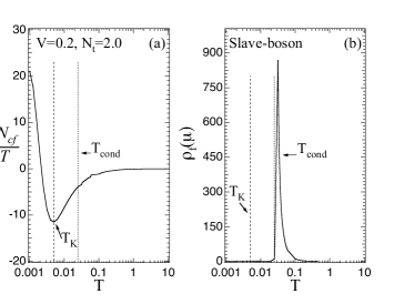
Figure 5: The temperature dependence of (a) $dN_{cf}/dT$ and (b) $\rho_{f}(\mu)$ in the MFSBT for $V=0.2$ and $N_{t}=2.0$. The vertical dashed line indicates $T_{K}$ and the vertical short dashed line indicates $T_{\mbox{\scriptsize{cond}}}$. Other parameters are the same as in Fig. 1.

For occupations in which $T=T_{\mbox{\scriptsize{cond}}}$ exists in the slave-boson approach, our data has always a global minimum for $dN_{cf}/dT$ in the interval $T<T_{\mbox{\scriptsize{cond}}}$, as can be seen in Fig. 5.a for $N_{t}=2.0$ and $V=0.2$. At $T=0.001$, we have that $g=46.17$ in the slave-boson approach, corresponding to an IV regime. Indeed, as can be seen in Fig. 5.b, the system is an insulator and several Kondo insulators present the same type of behavior.

Figure 6: The temperature dependence of (a) $dN_{cf}/dT$, (b) $\rho_{f}(\mu)$, and ${\rho^{\prime}}_{c}(\mu)=10\rho_{c}(\mu)$ in the MFXBT for $V=0.2$ and $N_{t}=1.6651$. The vertical dashed lines indicates $T_{K}$. Other parameters are the same as in Fig. 1.

These data should be compared with the results obtained for $N_{t}=1.6651$ and $V=0.2$ in the MFXBT, where the system is also an insulator at this occupation, in which $g=2.14$ at $T=0.001$. From Fig. 6 we can then infer that both the X-boson and the slave-boson approaches yield the same qualitative description for the system, but in the X-boson approach we do not have the spurious second-order phase transition presented by the MFSBT at $T=T_{\mbox{\scriptsize{cond}}}$.

5 Kondo Regime

To investigate the Kondo regime of the system, we vary the bare energy $E_{f}$ from the empty dot regime ($E_{f}>\mu$) to the extreme Kondo limit, where $E_{f}<<\mu$. As $E_{f}$ goes to the Kondo limit the charge fluctuations are suppressed, while the spin fluctuations become dominant. In the numerical calculations of this section we always employ the total occupation number $N_{t}=1.3$ and the hybridization $V=0.20$, and we calculate the chemical potential self-consistently. In the curves of density of states we give the frequencies with respect to the chemical potential, so that always is $\mu=0$. Also note that for the MFSBT we shall plot the “real” particle density of states, $\rho^{\mbox{\scriptsize{real}}}_{f}(\mu)=z\rho_{f}(\mu)$, where $\rho_{f}(\mu)$ is the quasi-particle density of states described by the usual fermionic operators in the MFSBT. For simplicity we shall suppress the “real” superscript along this section.

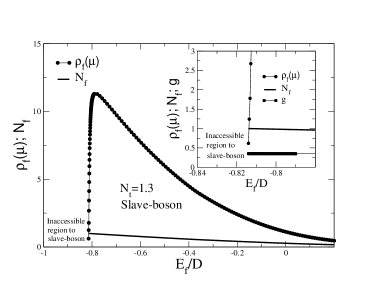
Figure 7: The spectral density $\rho_{f}(\mu)$ of local states and the total number of particles $N_{f}$ as a function of the position of the bare local level $E_{f}$ in the MFSBT, for $V=0.2$ and $N_{t}=1.3$ and $T=10^{-5}$. The inset shows the point where $\rho_{f}(\mu)\rightarrow 0$ and $N_{f}\rightarrow 1$.

The MFSBT results at $T=10^{-5}$ are shown in figure 7. As can be seen in the figure, $\rho_{f}(\mu)$ reaches a peak as $E_{f}$ decreases, denoting the enhancement of the effective mass of the system and its heavy fermion behavior due to the Kondo effect. As $E_{f}$ decreases even more, the $f$-density of states at the Fermi level falls steeply. The inset indeed shows that $\rho_{f}(\mu)\rightarrow 0$ when the $f$-band occupation $N_{f}$ approaches unity, i.e. the Kondo limit in the slave-boson approach, as already discussed above. Moreover, as $E_{f}$ decreases even more, we reach an interval where $z<0$, corresponding to unphysical results of the MFSBT, i.e. to an inaccessible region for the slave-boson method.

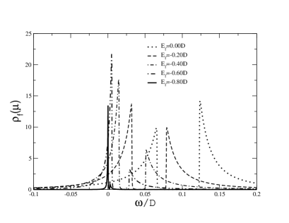
Figure 8: The spectral localized density of states $\rho_{f}(\omega)$ as a function of the frequency $\omega$ in the MFSBT employing the same values used in Fig. 7.

Fig. 8 shows the $f$-band densities of states as a function of $\omega$ (taking the chemical potential at the origin). The hybridization gap goes to zero at the Kondo limit, and the first peak of the density of states mimics the lattice Kondo peak.

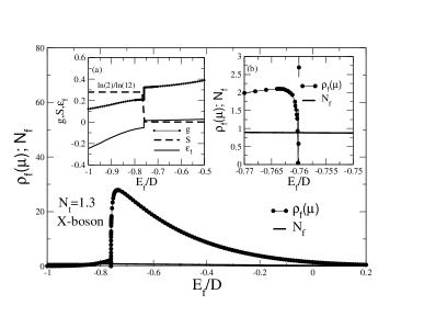
Figure 9: The spectral localized density of states $\rho_{f}(\mu)$, and $N_{f}$ as a function of the position of the localized level $E_{f}$ in the MFXBT employing the same values used in figure 7. The inset $(a)$ shows a detail of the parameter $g$, the entropy $S$ and the localized level $\epsilon_{f}=E_{f}-\mu$ in the region of the transition from the HF-K to LMM regime. The inset $(b)$ shows the behavior of the $\rho_{f}(\mu)$ and $n_{f}$ around the transition.

On the same token, the MFXBT results for $N_{t}=1.3$ and $V=0.2$ are shown in figure (9). The X-boson results are similar to those obtained in the MFSBT: $\rho_{f}(\mu)$ reaches a peak as $E_{f}$ decreases, denoting the effective mass enhancement of the heavy fermions, and if further decreases when the $E_{f}$ decreases even more. In the inset (a) we plot the parameter $g$, the entropy $S$ and the localized level $\epsilon_{f}=E_{f}-\mu$ as function of $E_{f}$, and all these quantities present a steeply but continuous behavior at $E_{f}\approx-0.76$. We identify this “jump” as the transition from the heavy Fermion Kondo regime (HF-K) to the local magnetic moment regime (LMM). As pointed out by Steglich [18], in real systems, the majority of HF-K compounds is found in the region where $g<g_{c}$ and these systems suffer a magnetic phase transition before both the heavy masses and coherence among the quasiparticles can fully develop. The results obtained by the X-boson are consistent with this scenario, but here we do not calculate magnetic solutions of the problem; we can only say that in the LMM phase the system presents an effective mass which is lower than in the HF-Kondo regime, as indicated by the specific heat $\gamma$ coefficient calculation [10]. Considering the Kondo and RKKY energies, since $k_{B}T_{RKKY}\sim g^{2}$ and $k_{B}T^{cond}\sim\exp(-1/g)$ respectively, we obtain that the $E_{f}$ value when the Kondo and the RKKY interactions have the same strength, occurs at around the $E_{f}$ critical transition value, what leads us to consider this region as “associated”, in a mean field way, to the critical parameter $g_{c}$, as discussed in the end of the Section 3. Nevertheless, we should be cautious about this result, since the X-boson is only a mean field theory and within this formalism it is not possible to capture all the relevant physics associated to this transition. It is believed that this transition defines a Quantum Critical Point (QCP) [5]. However, given that the X-boson self-energy does not depend on the wave vector, we cannot take into consideration the RKKY interaction and we cannot discuss the non-Fermi liquid behavior, nor find the correct $g_{c}$ value associated with the QCP. As can be seen in the inset (a), the entropy $S$ per site in the HF-K regime is close to zero, signaling the Kondo singlet ground-state; however, as $\mu$ crosses the hybridization gap and $E_{f}$ decreases even more, $S$ presents a continuous transition at $E_{f}\approx-0.76$. In the LMM region, $S\rightarrow k_{B}ln(2)/ln(12)$, with $k_{B}=1$ in all the calculations, pointing to the transformation of the singlet of the HF-K regime into a ground state consisting of a doublet at each site, that could be attributed to a spin $1/2$ at each site, which is the LMM regime presented by the PAM when $N_{f}\rightarrow 1$. This regime cannot be obtained in the slave-boson approach. This transition always appears in the Kondo region, when the chemical potential $\mu$ changes signal forcing the localized level $\epsilon_{f}=E_{f}-\mu$ to enter the LMM region, as represented in the inset (a) of the Fig. (9). In the inset (b), we present a detail of $\rho_{f}(\mu)$, and $N_{f}$ as a function of the position of the localized level$E_{f}$. The two methods give qualitatively different results in this region: while the slave boson reproduces the impurity Kondo limit the X-boson gives a transition to the LMM regime, which is essentially a lattice behavior as can be inferred by several experimental results [1, 18].

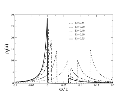
Figure 10: The spectral localized density of states $\rho_{f}(\omega)$ as a function of the frequency $\omega$ in the MFXBT employing the same values used in Fig. 7.

Fig. 10 shows the $f$-band densities of states as a function of $\omega$ (taking the chemical potential at the origin) in the MFXBT. As in the slave-boson approach, the density of states exhibits a double-peak structure for every value of $E_{f}$, but now the hybridization gap does not goes to zero as in the slave boson case. The first peak is enhanced at $\mu=0$, which mimics again the Kondo peak, and at the same time the second peak loses importance.

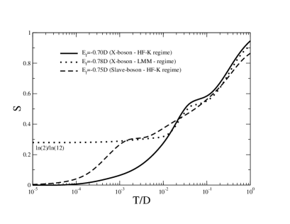
Figure 11: Entropy $S$ as a function of the temperature $T$ in the MFXBT and MFSBT for several values of $E_{f}$ using $N_{t}=1.3$ and $V=0.2$.

in Fig. 11 we present the calculation of the entropy [10] as a function of the temperature for both the slave-boson and the X-boson methods. For a system with a chemical potential that remains finite when $T\rightarrow\infty$, the entropy per site would tend to $k_{B}\ ln(12)$, corresponding to the dimensionality of the purely local Hilbert space. The results for $E_{f}=-0.70$ in the X-boson and for $-0.75$ in the slave-boson approach, show that $S$ tends to zero as $T\rightarrow 0$, indicating that the system in the ground-state goes to the Kondo singlet. However, in the MFXBT, the entropy $S$ per site for $E_{f}=-0.78$ tends in the low temperatures limit to $k_{B}ln(2)/ln(12)$, indicating a ground state consisting of a doublet at each site.

6 Conclusions

In this paper we have employed both the MFSBT and the MFXBT to study the paramagnetic case of the PAM in the limit $U=\infty$, and we have compared their results and predictions.

As we pointed earlier there is a belief in the literature that, for the lattice case, the collapse of the quasi-particles bands in the MFSBT, occurs only at very high temperatures, in contrast with the impurity case where this breakdown occurs at the condensation temperature $T_{cond}$ (see reference [3] - pg. $343$). But the results summarized in figure 1, shows that for the lattice case, the MFSBT present a more complex behavior. Within the MFSBT, we have defined a temperature $T_{\mbox{\scriptsize{cond}}}$ at which the average occupation $z$ of the vacuum state is $z=0$, and we have calculated numerically the temperature dependence of $z$ for a constant total number of electrons $N_{t}$. Our results show that: in the low occupations regime, the system never reaches $T=T_{\mbox{\scriptsize{cond}}}$ at constant $N_{t}$, although previous calculations [8] for a constant $\mu$ always present the spurious phase transition at $z=0$; for a range of occupations $N_{t}\lesssim 2$, there are two values of $T$ where $z=0$: $z$ is positive up to $T=T_{\mbox{\scriptsize{cond}}}$, and it then becomes negative for a bounded temperature interval. As $T$ increases even more, $z=1-N_{f}$ becomes positive again, to satisfy the high-temperatures result $N_{c}=N_{f}$, shown in Appendix B; in the high occupations regime, $z$ is negative for every range of temperatures. Finally, from the Appendix B we prove that the high temperature limit of the MFSBT determines completely the strange behavior of the condensation temperature in the lattice case.

In order to avoid these problems, we study the PAM employing the MFXBT, which does not have these difficulties of the slave-boson method, giving $N_{f}<1$ for every range of temperatures and occupations, as should be expected for the PAM in the $U=\infty$ limit. Moreover, the $c$-band and $f$-band densities of states at the chemical potential are always positive, showing that the X-boson approach provides physical results for every range of temperatures and occupations. In the Kondo limit both methods present similar results but the entropy data in the MFXBT results shows a steeply but continuous transition where the singlet of the heavy fermion Kondo regime transforms into a ground state consisting of a doublet at each site, that could be attributed to a spin $1/2$ at each site, which is the local magnetic moment regime presented by the PAM. This regime cannot be obtained by the slave-boson approach.

As the final conclusions we can say that the X-boson plays a complementary role when compared with the slave boson approach which was designed to describe the Kondo limit of the PAM, but fails as the temperature increases. On the other hand, since the computational costs of the X-boson is equivalent to the slave-boson and produces physical results for the PAM at any temperature or chemical potential, this approach seems useful as a starting point to study temperature dependent problems of heavy fermion systems like heavy fermion superconductivity [20, 21, 22], intermediate valence systems like the Kondo insulators [23] or the transition to HF-K to LMM regime [1, 18].

Appendix A The condensation temperature

We shall call $T_{\mbox{\scriptsize{cond}}}$ the temperature at which the system takes the value $z=0$ in the MFSBT. The constrain 2 to the Hilbert space gives, $z+{\mathcal{N}_{s}}^{-1}\sum_{\mathbf{k},\sigma}\langle f_{\mathbf{k,\sigma}}^{\dagger}f_{\mathbf{k}\sigma}\rangle=1$, the $T_{\mbox{\scriptsize{cond}}}$ can be reached if, and only if, $N_{f}=1$. When $z\rightarrow 0$ it follows $\tilde{V}=\sqrt{z}\ V\rightarrow 0$, and from (4) we have ${\mathcal{G}}_{\sigma}^{f}(\mathbf{k},\omega)\equiv-1/\left(i\omega-\tilde{E_{f}}\right)\,$, so that $N_{f}=N_{\sigma}n_{F}(\tilde{E_{f}})$, where $N_{\sigma}=2$ is the number of spin components. The relation $N_{f}=1$ then implies $\tilde{E_{f}}=0$, and we obtain $T_{\mbox{\scriptsize{cond}}}$ by taking simultaneously $z=0$ and $\tilde{E_{f}}=0$.

With the same procedure employed in [8] we obtain

$$\lambda=-V^{2}N_{\sigma}\int d\epsilon\rho(\epsilon)\,\frac{n_{F}\left(\omega_{+}\right)-n_{F}\left(\omega_{-}\right)}{\omega_{+}-\omega_{-}}\,,$$ (14)

where $n_{F}(x)\equiv\left(1+e^{\beta x}\right)^{-1}$ is the Fermi function. This equation is analogous to the (12) in the X-boson approach. At $T=T_{\mbox{\scriptsize{cond}}}$, we get that $\lambda=\mu-E_{f}$, and (14) can be rewritten as

$$1=\frac{N_{\sigma}V^{2}}{2\left(\mu-E_{f}\right)}\int d\epsilon\,\rho(\epsilon)\frac{1-2n_{F}(\epsilon-\mu)}{\epsilon-\mu}\,,$$ (15)

which is a self-consistent equation for $T_{\mbox{\scriptsize{cond}}}$. Using the density of states in (6) and integrating (15) by parts in the weak-coupling limit, $D-\mu\gg k_{B}T_{\mbox{\scriptsize{cond}}}$, we get that [24]

$$k_{B}T_{\mbox{\scriptsize{cond}}}=\frac{2e^{\gamma}}{\pi}\left(D-\mu\right)\exp\left[-D\frac{\mu-E_{f}}{V^{2}}\right]\,,$$ (16)

where $\gamma$ is the Euler’s constant and $N_{\sigma}=2$ in our model Hamiltonian.

Appendix B High temperature limit

      

Figure 12: Temperature dependence of $N_{f}$ and $N_{c}$ for $N_{t}=2.2$ (a) in the slave-boson approach and (b) in the X-boson approach. Other parameters are the same as in Fig. 1.

In Section 2 we have stated that for intermediate values of $N_{t}$, but for $N_{t}<2$ (represented by $N_{t}=1.95$ in Fig. 1), $z$ is negative at a finite interval only, becoming positive again at a sufficiently high temperature. This follows in the MFSBT because $N_{f}=N_{c}$ in the high temperature regime, and from $N_{t}=N_{f}+N_{c}<2$ we obtain $N_{f}<1$, so that $z$ is positive.

First note that the occupations $N_{c}$ and $N_{f}$ are written as

$$N_{f,c}=N_{\sigma}\int d\epsilon\,\rho(\epsilon)\left[A^{f,c}n_{F}(\omega_{+})+B^{f,c}n_{F}(\omega_{-})\right]\,,$$ (17)

where

$$A^{f}=\frac{E_{\mathbf{k}}-\omega_{+}}{\omega_{-}-\omega_{+}}\;,\;B^{f}=\frac{\omega_{-}-E_{\mathbf{k}}}{\omega_{-}-\omega_{+}}\,,$$ (18)

$$A^{c}=\frac{\tilde{E_{f}}-\omega_{+}}{\omega_{-}-\omega_{+}}\;,\;B^{c}=\frac{\omega_{-}-\tilde{E_{f}}}{\omega_{-}-\omega_{+}}\,,$$ (19)

and $N_{\sigma}$ is the number of spin components per state $k$.

¿From (5) we can write $\omega_{\pm}=-\mu+\phi_{\pm}$, with

$$\phi_{\pm}=\frac{1}{2}\left\{\epsilon_{\mathbf{k}}+\left(E_{f}+\lambda\right)\pm\sqrt{\left[\epsilon_{\mathbf{k}}-\left(E_{f}+\lambda\right)\right]^{2}+4\tilde{V}^{2}}\right\}\,,$$ (20)

where $\phi_{\pm}$ are the true energies of the quasi-particles in the Hamiltonian in (3) before subtracting the quantity $\mu\left\{\sum_{\mathbf{j},\sigma}f_{\mathbf{j},\sigma}^{\dagger}f_{\mathbf{j},\sigma}+\sum_{\mathbf{k},\sigma}c_{\mathbf{k},\sigma}^{\dagger}c_{\mathbf{k},\sigma}\right\}$. As the $\phi_{\pm}$ are bounded, we have $\lim_{\beta\rightarrow 0}\exp\left(\beta\omega_{\pm}\right)=\exp\left(-\beta\mu\right)$. Hence, in the high-temperatures limit, (17) becomes

$$\lim_{\beta\rightarrow 0}N_{c}=\lim_{\beta\rightarrow 0}N_{f}=\frac{N_{\sigma}}{1+e^{-\beta\mu}}\,,$$ (21)

where we have made use of the relations $A^{c}+B^{c}=A^{f}+B^{f}=1$, which can be verified by inspection from (18) and (19). Further, from (21) above, it follows immediately that $\mu$ satisfies

$$N_{t}=2N_{\sigma}\left(1+e^{-\beta\mu}\right)^{-1}$$ (22)

in the high temperature limit.

Following the development above but with the GF corresponding to the MFXBT, one can calculate $N_{f}$ and $N_{c}$ in the high-temperatures limit for the X-boson approach. Indeed, from (11), $\omega_{\pm}^{\sigma}=-\mu+\phi_{\pm}^{\sigma}$ and since $N_{f}\leq 1$ in the MFXBT for every range of temperatures and occupations, we find that $D_{\sigma}$ is bounded, so that $\phi_{\pm}^{\sigma}$ is also bounded. Hence, $\lim_{\beta\rightarrow 0}\exp\left(\beta\omega_{\pm}^{\sigma}\right)=\exp\left(-\beta\mu\right)$ and for $N_{\sigma}=2$ in the high-temperatures limit we have

$$\lim_{\beta\rightarrow 0}N_{c}=\frac{2}{1+e^{-\beta\mu}}\;\;\mbox{ and }\;\;\lim_{\beta\rightarrow 0}N_{f}=D_{\sigma}\,\frac{2}{1+e^{-\beta\mu}}\,.$$ (23)

The presence of $D_{\sigma}$ in the GF given in (10) is reflected in (23), and replacing $D_{\sigma}=1-(N_{f}/2)$ in this last equation we find that

$$N_{f}=\frac{2}{2+e^{-\beta\mu}}\,,$$ (24)

which is identical to the result obtained in [10]. Therefore, $N_{f}\not=N_{c}$ for the X-boson approach in the high temperature limit. Indeed, Fig. 12 shows the temperature dependence of $N_{f}$ and $N_{c}$, for $N_{t}=2.2$. As $T$ increases, $N_{f}\rightarrow 1.1$ for the MFSBT, which is unacceptable in the $U=\infty$ limit. This result does not occur in the X-boson approach, as can be seen in Fig. 12.b.

References

- [1] N. Grewe and F. Steglich, 1991 Handbook on the Physics and Chemistry of Rare Earths 14 (1991) (edited by K A Gschneider and L Eyring Elsevier, Amsterdam).
- [2] P. Fulde, J. Keller and G. Zwicknagl Solid State Physics 41 (1988) 1.
- [3] A. C. Hewson, The Kondo Problem to Heavy Fermions (1993) (Cambridge University Press, New York).
- [4] G. Aeppli and Z. Fisk, Comments Cond. Mat. Phys. 16 (1992) 155.
- [5] M. A. Continentino, Quantum Scaling in Many Body Systems (2001) (World Scientific, Singapore).
- [6] P. Coleman, Phys. Rev. B 29 (1984) 3035.
- [7] P. Coleman, Phys. Rev. B 35 1987 5072.
- [8] R. Franco, M. S. Figueira and M. E. Foglio, Phys. Rev. B 66 (2002) 045112.
- [9] R. Franco, M. S. Figueira and M. E. Foglio, Physica A 308 (2002) 245.
- [10] R. Franco, M. S. Figueira and M. E. Foglio, Phys. Rev. B 68 (2003) 205108.
- [11] D. M. Newns and N. Read, Advances in Physics 36 (1987) 799.
- [12] S. Burdin, A. Georges and D. Grempel, Phys. Rev. Lett. 85 (2000) 1048.
- [13] B. H. Bernhard and C. Lacroix, Phys. Rev. B 60 (1999) 12149.
- [14] J. Hubbard, Proc. Royal Soc. A 276 (1964) 238.
-
[15]
M. S. Figueira, M. E. Foglio and G. G. Martinez, Phys. Rev. B 50 (1994) 17933;
M. E. Foglio and M. S. Figueira, J. Phys. A 30 (1997) 7879;
M. E. Foglio and M. S. Figueira, Int. J. of Mod. Phys. B 12 (1998) 837. - [16] M. S. Figueira and M. E. Foglio, J. Phys. Cond. Matter 8 (1996) 5017.
- [17] C. M. Varma, Comments on Condensed Matter Physics 11 (1985) 221.
- [18] F. Steglich, C. Geibel, K. Gloss, G. Olesch, C. Schank, C. Wassilew, A. Loidl, A. Krimmel and G. R. Stewart, J. Low Temp. Phys. 95 (1994) 3.
- [19] J. R. Schrieffer and P. A. Wolff, Phys. Rev. 149 (1966) 491.
- [20] L. H. C. M. Nunes, M. S. Figueira and E. V. L. Mello, Phys. Rev. B 68 (2003) 134511.
- [21] L. H. C. M. Nunes, M. S. Figueira and E. V. L. Mello, Physica C 408-410 (2004) 181.
- [22] L. H. C. M. Nunes, M. S. Figueira and E. V. L. Mello, J. Magn. Magn. Mat. 272-276 (2004) 148.
- [23] T. G. Rappoport, M. S. Figueira and M. A. Continentino, Physics Letters A 264 (2000) 497.
- [24] P. S. Riseborough, Phys. Rev. B 45 (1992) 13984.