Learning Set Functions that are Sparse in Non-Orthogonal Fourier Bases

Abstract

Many applications of machine learning on discrete domains, such as learning preference functions in recommender systems or auctions, can be reduced to estimating a set function that is sparse in the Fourier domain. In this work, we present a new family of algorithms for learning Fourier-sparse set functions. They require at most $nk-k\log_{2}k+k$ queries (set function evaluations), under mild conditions on the Fourier coefficients, where $n$ is the size of the ground set and $k$ the number of non-zero Fourier coefficients. In contrast to other work that focused on the orthogonal Walsh-Hadamard transform (WHT), our novel algorithms operate with recently introduced non-orthogonal Fourier transforms that offer different notions of Fourier-sparsity. These naturally arise when modeling, e.g., sets of items forming substitutes and complements. We demonstrate effectiveness on several real-world applications.

1 Introduction

Numerous problems in machine learning on discrete domains involve learning set functions, i.e., functions $s:2^{N}\to\mathbb{R}$ that map subsets of some ground set $N$ to the real numbers. In recommender systems, for example, such set functions express diversity among sets of articles and their relevance w.r.t. a given need (Sharma, Harper, and Karypis 2019; Balog, Radlinski, and Arakelyan 2019); in sensor placement tasks, they express the informativeness of sets of sensors (Krause, Singh, and Guestrin 2008); in combinatorial auctions, they express valuations for sets of items (Brero, Lubin, and Seuken 2019). A key challenge is to estimate $s$ from a small number of observed evaluations. Without structural assumptions an exponentially large (in $n=|N|$) number of queries is needed. Thus, a key question is which families of set functions can be efficiently learnt, while capturing important applications. One key property is sparsity in the Fourier domain (Stobbe and Krause 2012; Amrollahi et al. 2019).

The Fourier transform for set functions is classically known as the orthogonal Walsh-Hadamard transform (WHT) (Bernasconi, Codenotti, and Simon 1996; De Wolf 2008; Li and Ramchandran 2015; Cheraghchi and Indyk 2017). Using the WHT, it is possible to learn functions with at most $k$ non-zero Fourier coefficients with $O(nk)$ evaluations (Amrollahi et al. 2019). In this paper, we consider an alternative family of non-orthogonal Fourier transforms, recently introduced in the context of discrete signal processing on set functions (DSSP) (Püschel 2018; Püschel and Wendler 2020). In particular, we present the first efficient algorithms which (under mild assumptions on the Fourier coefficients), efficiently learn $k$-Fourier-sparse set functions requiring at most $(n+1)k-k\log_{2}k$ evaluations. In contrast, naively computing the Fourier transform requires $2^{n}$ evaluations and $n2^{n-1}$ operations (Püschel and Wendler 2020).

Importantly, sparsity in the WHT domain does not imply sparsity in the alternative Fourier domains we consider, or vice versa. Thus, we significantly expand the class of set functions that can be efficiently learnt. One natural example of set functions, which are sparse in one of the non-orthogonal transforms, but not for the WHT, are certain preference functions considered by Djolonga, Tschiatschek, and Krause (2016) in the context of recommender systems and auctions. In recommender systems, each item may cover the set of needs that it satisfies for a customer. If needs are covered by several items at once, or items depend on each other to provide value there are substitutability or complementarity effects between the respective items, which are precisely captured by the new Fourier transforms (Püschel and Wendler 2020). Hence, a natural way to learn such set functions is to compute their respective sparse Fourier transforms.

Contributions. In this paper we develop, analyze, and evaluate novel algorithms for computing the sparse Fourier transform under various notions of Fourier basis:

1. We are the first to introduce an efficient algorithm to compute the sparse Fourier transform for the recent notions of non-orthogonal Fourier basis for set functions (Püschel and Wendler 2020). In contrast to the naive fast Fourier transform algorithm that requires $2^{n}$ queries and $n2^{n-1}$ operations, our sparse Fourier transform requires at most $nk-k\log_{2}k+k=O(nk-k\log k)$ queries and $O(nk^{2})$ operations to compute the $k$ non-zero coefficients of a Fourier-sparse set function. The algorithm works in all cases up to a null set of pathological set functions.

2. We then further extend our algorithm to handle an even larger class of Fourier-sparse set functions with $O(n^{2}k-nk\log k)$ queries and $O(n^{2}k+k^{2}n)$ operations using filtering techniques.

3. We demonstrate the effectiveness of our algorithms in three real-world set function learning tasks: learning surrogate objective functions for sensor placement tasks, learning facility locations functions for water networks, and preference elicitation in combinatorial auctions. The sensor placements obtained by our learnt surrogates are indistinguishable from the ones obtained using the compressive sensing based WHT by Stobbe and Krause (2012). However, our algorithm does not require prior knowledge of the Fourier support and runs significantly faster. The facility locations function learning task shows that certain set functions are sparse in the non-orthogonal basis while being dense in the WHT basis. In the preference elicitation task also only half as many Fourier coefficients are required in the non-orthogonal basis as in the WHT basis, which indicates that bidders’ valuation functions are well represented in the non-orthogonal basis.

Because of the page limit, all proofs are in the supplementary material.

2 Fourier Transforms for Set Functions

We introduce background and definitions for set functions and associated Fourier bases, following the discrete-set signal processing (DSSP) introduced by (Püschel 2018; Püschel and Wendler 2020). DSSP generalizes key concepts from classical signal processing, including shift, convolution, and Fourier transform to the powerset domain. The approach follows a general procedure that derives these concepts from a suitable definition of the shift operation (Püschel and Moura 2008).

Set functions. We consider a ground set $N=\{x_{1},\dots,x_{n}\}$. An associated set function maps each subset of $N$ to a real value:

$$s:2^{N}\to\mathbb{R};A\mapsto s\left(A\right).$$ (1)

Each set function can be identified with a $2^{n}$-dimensional vector $\mathbf{s}=(s\left(A\right))_{A\subseteq N}$ by fixing an order on the subsets. We choose the lexicographic order on the set indicator vectors.

Shifts. Classical convolution (e.g., on images) is associated with the translation operator. Analogously, DSSP considers different versions of "set translations", each yielding a different DSSP model, numbered 1–5. One choice is

$$\text{(model 4)}\quad T_{Q}s\left(A\right)=s\left(A\cup Q\right),\text{ for }Q\subseteq N.$$ (2)

The shift operators $T_{Q}$ are parameterized by the powerset monoid $(2^{N},\cup)$, since the equality $T_{Q}(T_{R}s)=T_{Q\cup R}s$ holds for all $Q,R\subseteq N$, and $s\in\mathbb{R}^{2^{N}}$.

Convolutional filters. The corresponding linear, shift-equivariant convolution in model 4 is given by

$$(h*s)\left(A\right)=\sum_{Q\subseteq N}h\left(Q\right)s\left(A\cup Q\right).$$ (3)

Namely, $(h*T_{R}s)\left(A\right)=T_{R}(h*s)\left(A\right)$, for all $R\subseteq N$. Convolving with $h$ is a linear mapping called a filter and $h$ is also a set function. In matrix notation we have $\mathbf{h*s}=H\mathbf{s}$, where $H$ is the filter matrix.

Fourier transform and convolution theorem. The Fourier transform (FT) simultaneously diagonalizes all filters, i.e., the matrix $FHF^{-1}$ is diagonal for all filter matrices $H$, where $F$ denotes the matrix form of the Fourier transform. Thus, different definitions of set shifts yield different notions of Fourier transform. For the shift in (2) the Fourier transform of $s$ takes the form

$$\widehat{s}\left(B\right)=\sum_{A\subseteq N:A\cup B=N}(-1)^{|A\cap B|}s\left(A\right)$$ (4)

with the inverse

$$s\left(A\right)=\sum_{B\subseteq N:A\cap B=\emptyset}\widehat{s}\left(B\right).$$ (5)

As a consequence we obtain the convolution theorem

$$\widehat{(h*s)}\left(B\right)=\overline{h}\left(B\right)\widehat{s}\left(B\right).$$ (6)

Interestingly, $\overline{h}$ (the so-called frequency response) is computed differently than $\widehat{s}$, namely as

$$\overline{h}\left(B\right)=\sum_{A\subseteq N:A\cap B=\emptyset}h\left(A\right).$$ (7)

In matrix form, with respect to the chosen order of $\mathbf{s}$, the Fourier transform and its inverse are

$$F=\begin{pmatrix}0&\phantom{-}1\\ 1&-1\\ \end{pmatrix}^{\otimes n}\quad\text{and}\quad F^{-1}=\begin{pmatrix}1&1\\ 1&0\\ \end{pmatrix}^{\otimes n},$$ (8)

respectively, in which $M^{\otimes n}=M\otimes\cdots\otimes M$ denotes the $n$-fold Kronecker product of the matrix $M$. Thus, the Fourier transform $\widehat{\mathbf{s}}=F\mathbf{s}$ and its inverse $\mathbf{s}=F^{-1}\widehat{\mathbf{s}}$ can be computed in $n2^{n-1}$ operations.

The columns of $F^{-1}$ form the Fourier basis and can be viewed as indexed by $B\subseteq N$. The $B$-th column is given by $\mathbf{f}^{B}_{A}=\iota_{A\cap B=\emptyset}$, where $\iota_{A\cap B=\emptyset}=1$ if $A\cap B=\emptyset$ and $\iota_{A\cap B=\emptyset}=0$ otherwise. The basis is not orthogonal as can be seen from the triangular structure in (8).

Example and interpretation. We consider a special class of preference functions that, e.g., model customers in a recommender system (Djolonga, Tschiatschek, and Krause 2016). Preference functions naturally occur in machine learning tasks on discrete domains such as recommender systems and auctions, in which, for example, they are used to model complementary- and substitution effects between goods. Goods complement each other when their combined utility is greater than the sum of their individual utilities. Analogously, goods substitute each other when their combined utility is smaller than the sum of their individual utilities. Formally, a preference function is given by

$$p(A) =\sum_{i\in A}u_{i}+\sum_{\ell=1}^{L}\left(\max_{i\in A}r_{\ell i}-\sum_{i\in A}r_{\ell i}\right)$$ (9)

$$\ \ -\sum_{k=1}^{K}\left(\max_{i\in A}a_{ki}-\sum_{i\in A}a_{ki}\right).$$

Equation (9) is composed of a so-called modular term parametrized by $u\in\mathbb{R}^{n}$, a repulsive term parametrized by $r\in\mathbb{R}_{\geq 0}^{L\times n}$, with $L\in\mathbb{N}$, and an attractive term parametrized by $a\in\mathbb{R}_{\geq 0}^{K\times n}$, with $K\in\mathbb{N}$. The repulsive term captures substitution and the attractive term complementary effects.

Example 1 (Running example).

Consider the ground set $\{x_{1},x_{2},x_{3}\}$, in which $x_{1}$ represents a tablet, $x_{2}$ a laptop and $x_{3}$ a tablet pen. Now, we create a preference function with a substitution effect between the laptop and the tablet which is expressed in the repulsive term $r=(2,2,0)$ and a complementary effect between the tablet and the tablet pen which is expressed in the attractive term $a=(1,0,1)$. The individual values of the items are expressed in the modular term $u=(2,2,1)$. As a result we get the following preference function $p$ and also show its Fourier transform $\widehat{p}$:

	$\emptyset$	$\{x_{1}\}$	$\{x_{2}\}$	$\{x_{1},x_{2}\}$	$\{x_{3}\}$	$\{x_{1},x_{3}\}$	$\{x_{2},x_{3}\}$	$\{x_{1},x_{2},x_{3}\}$
$p$	0	2	2	2	1	4	3	4
$\widehat{p}$	4	-1	0	-2	-2	1	0	0

Namely, as desired, $p\left(\{x_{1},x_{2}\}\right)<p\left(\{x_{1}\}\right)+p\left(\{x_{2}\}\right)$ and $p\left(\{x_{1},x_{3}\}\right)>p\left(\{x_{1}\}\right)+p\left(\{x_{3}\}\right)$. Note that $\widehat{p}$ is sparse. Next, we show this is always the case.

Lemma 1.

Preference functions of the form (9) are Fourier-sparse w.r.t. model 4 with at most $1+n+Ln+Kn$ non-zero Fourier coefficients.

Motivated by Lemma 1, we call set functions that are Fourier-sparse w.r.t. model 4 generalized preference functions. Formally, a generalized preference function is defined in terms of a collection of distinct subsets $N=\{S_{1},\dots,S_{n}\}$ of some universe $U:S_{i}\subseteq U$, $i\in\{1,\dots,n\}$, and a weight function $w:U\to\mathbb{R}$. The weight of a set $S\subseteq U$ is $\mathbf{w}(S)=\sum_{u\in S}w(u)$. Then, the corresponding generalized preference function is

$$s:2^{N}\to\mathbb{R};A\mapsto\mathbf{w}\left(\bigcup_{S_{i}\in A}S_{i}\right).$$ (10)

For non-negative weights $s$ is called a weighted coverage function (Krause and Golovin 2014), but here we allow general (signed) weights. Thus, generalized preference functions are generalized coverage functions as introduced in (Püschel and Wendler 2020). Generalized coverage functions can be visualized by a bipartite graph, see Fig. 1(a). In recommender systems, $S_{i}$ could model the customer-needs covered by item $i$. Then, the score that a customer associates to a set of items corresponds to the needs covered by the items in that set. Substitution as well as complementary effects occur if the needs covered by items overlap (e.g., $S_{i}\cap S_{j}\neq\emptyset$).

Concretely, we observe in Fig. 1(a) that in our running example the tablet and the laptop share one need with a positive sign which yields the substitution effect, and the tablet and the tablet pen share a need with a negative sign which yields the complementary effect.

(a) Coverage function

(b) Fourier transform in (4)

Figure 1: Preference function $p$ from Example 1 as generalized coverage function visualized as bipartite graph (a) and as Venn diagram (b). The Fourier coefficients are the weights of the fragments. Here, three are zero.

Interestingly, the Fourier coefficients for model 4 in (4) of a generalized coverage function are

$$\widehat{s}\left(B\right)=\begin{cases}\sum_{u\in U}w(u),&\text{if }B=\emptyset,\\ -\mathbf{w}\left(\bigcap_{S_{i}\in B}S_{i}\setminus\bigcup_{S_{i}\in N\setminus B}S_{i}\right),&\text{otherwise,}\end{cases}$$ (11)

which corresponds to the weights of the fragments of the Venn-diagram of the sets $S_{i}$ (Fig. 1(b)). If the universe $U$ contains fewer than $2^{n}$ items, some fragments will have weight zero, i.e., are Fourier-sparse. We refer to Section VIII of Püschel and Wendler (2020) for an in-depth discussion and interpretation of the spectrum (11).

$\begin{array}[]{@{}l llll@{}}\hline\cr\hline\cr&\text{shift }T_{Q}s\left(A\right)&F\text{ (sum)}:\widehat{s}\left(B\right)=&F^{-1}\text{ (sum)}:{s}_{A}=\\ \hline\cr 3&s\left(A\setminus Q\right)&\displaystyle\sum_{\stackrel{{\scriptstyle A\subseteq B}}{{\hphantom{A\cup B=N}}}}(-1)^{|A|}s\left(A\right)&\hphantom{\tfrac{1}{2^{n}}}\displaystyle\sum_{\stackrel{{\scriptstyle B\subseteq A}}{{\hphantom{A\cap B=\emptyset}}}}(-1)^{|B|}\widehat{s}\left(B\right)\\ 4&s\left(A\cup Q\right)&\displaystyle\sum_{\stackrel{{\scriptstyle A\subseteq N:}}{{A\cup B=N}}}(-1)^{|A\cap B|}s\left(A\right)&\hphantom{\tfrac{1}{2^{n}}}\displaystyle\sum_{\stackrel{{\scriptstyle B\subseteq N:}}{{A\cap B=\emptyset}}}\widehat{s}\left(B\right)\\ 5&s\left(A\setminus Q\cup Q\setminus A\right)&\displaystyle\sum_{\stackrel{{\scriptstyle A\subseteq N}}{{\hphantom{A\cup B=N}}}}(-1)^{|A\cap B|}s\left(A\right)&\tfrac{1}{2^{n}}\displaystyle\sum_{\stackrel{{\scriptstyle B\subseteq N}}{{\hphantom{A\cap B=\emptyset}}}}(-1)^{|A\cap B|}\widehat{s}\left(B\right)\\ \hline\cr\hline\cr\end{array}$

Table 1: Shifts and Fourier concepts.

Other shifts and Fourier bases. As mentioned before, Püschel and Wendler (2020) considers 5 types of shift, i.e. DSSP models, each with its respective shift-equivariant convolution, associated Fourier basis, and thus notion of Fourier-sparsity. Model 5 is the classical definition that yields the WHT and model 4 the version introduced above. Table 1 collects the key concepts, also including model 3.

The notions of Fourier-sparsity differ substantially between models. For example, consider the coverage function for which there is only one element in the universe $U$ and this element is covered by all sets $S_{1},\dots,S_{n}$. Then, $\widehat{s}\left(\emptyset\right)=1$, $\widehat{s}\left(N\right)=-1$ and $\widehat{s}\left(B\right)=0$ for $\emptyset\subset B\subset N$ w.r.t. model 4, and $\widehat{s}\left(\emptyset\right)=2^{n}-1$ and $\widehat{s}\left(B\right)=-1$ for all $\emptyset\subset B\subseteq N$ w.r.t. the WHT.

More generally, one can show that preference functions in (9) with at least one row of pairwise distinct values in either the repulsive or attractive part are dense w.r.t. the WHT basis.

The Fourier bases have appeared in different contexts before. For example, (4) can be related to the W-transform, which has been used by Chakrabarty and Huang (2012) to test coverage functions.

3 Learning Fourier-Sparse Set Functions

We now present our algorithm for learning Fourier-sparse set functions w.r.t. model 4. One of our main contributions is that the derivation and algorithm are general, i.e., they also applies to the other models. We derive the variants for models 3 and 5 from Table 1 in the supplementary material.

Definition 1.

A set function $s$ is called $k$-Fourier-sparse if

$$\operatorname{supp}(\widehat{s})=\{B:\widehat{s}\left(B\right)\neq 0\}=\{B_{1},\dots,B_{k}\},$$ (12)

where we assume that $k$ is significantly smaller than $2^{n}$.

Thus, exactly learning a $k$-Fourier-sparse set function is equivalent to computing its $k$ non-zero Fourier coefficients and associated support. Formally, we want to solve:

Problem 1 (Sparse FT).

Given oracle access to query a $k$-Fourier-sparse set function $s$, compute its Fourier support and associated Fourier coefficients.

3.1 Sparse FT with Known Support

First, we consider the simpler problem of computing the Fourier coefficients if the Fourier support $\operatorname{supp}(\widehat{s})$ (or a small enough superset $\mathcal{B}\supseteq\operatorname{supp}(\widehat{s})$) is known. In this case, the solution boils down to selecting queries $\mathcal{A}\subseteq 2^{N}$ such that the linear system of equations

$$\mathbf{s}_{\mathcal{A}}=F^{-1}_{\mathcal{A}\mathcal{B}}\mathbf{\widehat{s}}_{\mathcal{B}},$$ (13)

admits a solution. Here, $\mathbf{s}_{\mathcal{A}}=(s\left(A\right))_{A\in\mathcal{A}}$ is the vector of queries, $F^{-1}_{\mathcal{A}\mathcal{B}}$ is the submatrix of $F^{-1}$ obtained by selecting the rows indexed by $\mathcal{A}$ and the columns indexed by $\mathcal{B}$, and $\mathbf{\widehat{s}}_{\mathcal{B}}$ are the unknown Fourier coefficients we want to compute.

Theorem 1 (Püschel and Wendler (2020)).

Let $s$ be $k$-Fourier-sparse with ${\operatorname{supp}(\widehat{s})=\{B_{1},\dots,B_{k}\}=\mathcal{B}}$. Let ${\mathcal{A}=\{N\setminus B_{1},\dots,N\setminus B_{k}\}}$. Then $F^{-1}_{\mathcal{A}\mathcal{B}}$ is invertible and $s$ can be perfectly reconstructed from the queries $\mathbf{s}_{\mathcal{A}}$.

Consequently, we can solve Problem 1 if we have a way to discover a $\mathcal{B}\supseteq\operatorname{supp}(\widehat{s})$, which is what we do next.

3.2 Sparse FT with Unknown Support

In the following we present our algorithm to solve Problem 1. As mentioned, the key challenge is to determine the Fourier support w.r.t. (4). The initial skeleton is similar to the algorithm Recover Coverage by Chakrabarty and Huang (2012), who used it to test coverage functions. Here we take the novel view of Fourier analysis to expand it to a sparse Fourier transform algorithm for all set functions. Doing so creates challenges since here the weight function in (10) is not guaranteed to be positive. Using the framework in Section 2 we will analyze and address them.

Let $M\subseteq N$, and consider the associated restriction of a set function $s$ on $N$:

$$s\downarrow_{2^{M}}:2^{M}\to\mathbb{R};A\mapsto s\left(A\right)$$ (14)

The Fourier coefficients of $s$ and the restriction can be related as (proof in supplementary material):

$$\savestack{\tmpbox}{\stretchto{\scaleto{\scalerel*[\widthof{s\downarrow_{2^{M}}}]{\kern-0.6pt\bigwedge\kern-0.6pt}{\rule[-650.43pt]{4.30554pt}{650.43pt}}}{}}{0.5ex}}\stackon[1pt]{s\downarrow_{2^{M}}}{\tmpbox}\left(B\right)=\sum_{A\subseteq N\setminus M}\widehat{s}\left(A\cup B\right).$$ (15)

We observe that, if the Fourier coefficients on the right hand side of (15) do not cancel, knowing $\savestack{\tmpbox}{\stretchto{\scaleto{\scalerel*[\widthof{s\downarrow_{2^{M}}}]{\kern-0.6pt\bigwedge\kern-0.6pt}{\rule[-650.43pt]{4.30554pt}{650.43pt}}}{}}{0.5ex}}\stackon[1pt]{s\downarrow_{2^{M}}}{\tmpbox}$ contains information about the sparsity of $\savestack{\tmpbox}{\stretchto{\scaleto{\scalerel*[\widthof{s\downarrow_{2^{M\cup\{x\}}}}]{\kern-0.6pt\bigwedge\kern-0.6pt}{\rule[-650.43pt]{4.30554pt}{650.43pt}}}{}}{0.5ex}}\stackon[1pt]{s\downarrow_{2^{M\cup\{x\}}}}{\tmpbox}$, for $x\in N\setminus M$. To be precise, if there are no cancellations, the relation

$$\savestack{\tmpbox}{\stretchto{\scaleto{\scalerel*[\widthof{s\downarrow_{2^{M}}}]{\kern-0.6pt\bigwedge\kern-0.6pt}{\rule[-650.43pt]{4.30554pt}{650.43pt}}}{}}{0.5ex}}\stackon[1pt]{s\downarrow_{2^{M}}}{\tmpbox}\left(B\right) =\savestack{\tmpbox}{\stretchto{\scaleto{\scalerel*[\widthof{s\downarrow_{2^{M\cup\{x\}}}}]{\kern-0.6pt\bigwedge\kern-0.6pt}{\rule[-650.43pt]{4.30554pt}{650.43pt}}}{}}{0.5ex}}\stackon[1pt]{s\downarrow_{2^{M\cup\{x\}}}}{\tmpbox}\left(B\right)+\savestack{\tmpbox}{\stretchto{\scaleto{\scalerel*[\widthof{s\downarrow_{2^{M\cup\{x\}}}}]{\kern-0.6pt\bigwedge\kern-0.6pt}{\rule[-650.43pt]{4.30554pt}{650.43pt}}}{}}{0.5ex}}\stackon[1pt]{s\downarrow_{2^{M\cup\{x\}}}}{\tmpbox}\left(B\cup\{x\}\right)$$ (16)

implies that both $\savestack{\tmpbox}{\stretchto{\scaleto{\scalerel*[\widthof{s\downarrow_{2^{M\cup\{x\}}}}]{\kern-0.6pt\bigwedge\kern-0.6pt}{\rule[-650.43pt]{4.30554pt}{650.43pt}}}{}}{0.5ex}}\stackon[1pt]{s\downarrow_{2^{M\cup\{x\}}}}{\tmpbox}\left(B\right)$ and $\savestack{\tmpbox}{\stretchto{\scaleto{\scalerel*[\widthof{s\downarrow_{2^{M\cup\{x\}}}}]{\kern-0.6pt\bigwedge\kern-0.6pt}{\rule[-650.43pt]{4.30554pt}{650.43pt}}}{}}{0.5ex}}\stackon[1pt]{s\downarrow_{2^{M\cup\{x\}}}}{\tmpbox}\left(B\cup\{x\}\right)$ must be zero whenever $\savestack{\tmpbox}{\stretchto{\scaleto{\scalerel*[\widthof{s\downarrow_{2^{M}}}]{\kern-0.6pt\bigwedge\kern-0.6pt}{\rule[-650.43pt]{4.30554pt}{650.43pt}}}{}}{0.5ex}}\stackon[1pt]{s\downarrow_{2^{M}}}{\tmpbox}\left(B\right)$ is zero. As a consequence, we can construct

$$\mathcal{B}=\bigcup_{B\in\operatorname{supp}(\savestack{\tmpbox}{\stretchto{\scaleto{\scalerel*[\widthof{s\downarrow_{2^{M}}}]{\kern-0.6pt\bigwedge\kern-0.6pt}{\rule[-650.43pt]{3.01389pt}{650.43pt}}}{}}{0.5ex}}\stackon[1pt]{s\downarrow_{2^{M}}}{\tmpbox})}\{B,B\cup\{x\}\},$$ (17)

with $\operatorname{supp}(\savestack{\tmpbox}{\stretchto{\scaleto{\scalerel*[\widthof{s\downarrow_{2^{M\cup\{x\}}}}]{\kern-0.6pt\bigwedge\kern-0.6pt}{\rule[-650.43pt]{4.30554pt}{650.43pt}}}{}}{0.5ex}}\stackon[1pt]{s\downarrow_{2^{M\cup\{x\}}}}{\tmpbox})\subseteq\mathcal{B}$, from (16), and then compute $\savestack{\tmpbox}{\stretchto{\scaleto{\scalerel*[\widthof{s\downarrow_{2^{M\cup\{x\}}}}]{\kern-0.6pt\bigwedge\kern-0.6pt}{\rule[-650.43pt]{4.30554pt}{650.43pt}}}{}}{0.5ex}}\stackon[1pt]{s\downarrow_{2^{M\cup\{x\}}}}{\tmpbox}$ with Theorem 1 in this case.

As a result we can solve Problem 1 with our algorithm SSFT, under mild conditions on the coefficients that guarantee that cancellations do not occur, by successively computing the non-zero Fourier coefficients of restricted set functions along the chain

$$s\downarrow_{2^{\emptyset}}=\savestack{\tmpbox}{\stretchto{\scaleto{\scalerel*[\widthof{s\downarrow_{2^{\emptyset}}}]{\kern-0.6pt\bigwedge\kern-0.6pt}{\rule[-650.43pt]{4.30554pt}{650.43pt}}}{}}{0.5ex}}\stackon[1pt]{s\downarrow_{2^{\emptyset}}}{\tmpbox},\savestack{\tmpbox}{\stretchto{\scaleto{\scalerel*[\widthof{s\downarrow_{2^{\{x_{1}\}}}}]{\kern-0.6pt\bigwedge\kern-0.6pt}{\rule[-650.43pt]{4.30554pt}{650.43pt}}}{}}{0.5ex}}\stackon[1pt]{s\downarrow_{2^{\{x_{1}\}}}}{\tmpbox},\savestack{\tmpbox}{\stretchto{\scaleto{\scalerel*[\widthof{s\downarrow_{2^{\{x_{1},x_{2}\}}}}]{\kern-0.6pt\bigwedge\kern-0.6pt}{\rule[-650.43pt]{4.30554pt}{650.43pt}}}{}}{0.5ex}}\stackon[1pt]{s\downarrow_{2^{\{x_{1},x_{2}\}}}}{\tmpbox},\dots,\savestack{\tmpbox}{\stretchto{\scaleto{\scalerel*[\widthof{s\downarrow_{2^{N}}}]{\kern-0.6pt\bigwedge\kern-0.6pt}{\rule[-650.43pt]{4.30554pt}{650.43pt}}}{}}{0.5ex}}\stackon[1pt]{s\downarrow_{2^{N}}}{\tmpbox}=\widehat{s}.$$ (18)

For example, SSFT works with probability one if all non-zero Fourier coefficients are sampled from independent continuous probability distributions:

Lemma 2.

With probability one SSFT correctly computes the Fourier transform of Fourier-sparse set functions $s$ with $\operatorname{supp}(\widehat{s})=\mathcal{B}$ and randomly sampled Fourier coefficients, that satisfy

1. $\widehat{s}\left(B\right)\sim P_{B}$, where $P_{B}$ is a continuous probability distribution with density function $p_{B}$, for $B\in\operatorname{supp}(\widehat{s})$,

2. $p_{\mathcal{B}}=\prod_{B\in\mathcal{B}}p_{B}$.

SSFT Sparse set function Fourier transform of $s$

1:$M_{0}\leftarrow\emptyset$

2:$\savestack{\tmpbox}{\stretchto{\scaleto{\scalerel*[\widthof{s\downarrow_{2^{M_{0}}}}]{\kern-0.6pt\bigwedge\kern-0.6pt}{\rule[-650.43pt]{4.30554pt}{650.43pt}}}{}}{0.5ex}}\stackon[1pt]{s\downarrow_{2^{M_{0}}}}{\tmpbox}\left(\emptyset\right)\leftarrow s\left(\emptyset\right)$

3:for $i=1,\dots,n$ do

4:     $M_{i}\leftarrow M_{i-1}\cup\{x_{i}\}$

5:     $\mathcal{B}\leftarrow\emptyset,\mathcal{A}\leftarrow\emptyset$

6:     for $B\in\operatorname{supp}(\savestack{\tmpbox}{\stretchto{\scaleto{\scalerel*[\widthof{s\downarrow_{2^{M_{i-1}}}}]{\kern-0.6pt\bigwedge\kern-0.6pt}{\rule[-650.43pt]{4.30554pt}{650.43pt}}}{}}{0.5ex}}\stackon[1pt]{s\downarrow_{2^{M_{i-1}}}}{\tmpbox})$ do

7:         $\mathcal{B}\leftarrow\mathcal{B}\cup\{B,B\cup\{x_{i}\}\}$

8:         $\mathcal{A}\leftarrow\mathcal{A}\cup\{M_{i}\setminus B,M_{i}\setminus(B\cup\{x_{i}\})\}$      

9:     $\mathbf{s}_{\mathcal{A}}\leftarrow(s\left(A\right))_{A\in\mathcal{A}}$

10:     $\mathbf{x}\leftarrow\text{ solve }\mathbf{s}_{\mathcal{A}}=F^{-1}_{\mathcal{A}\mathcal{B}}\mathbf{x}$ for $\mathbf{x}$

11:     for $B\in\mathcal{B}$ with $\mathbf{x}_{B}\neq 0$ do

12:         $\savestack{\tmpbox}{\stretchto{\scaleto{\scalerel*[\widthof{s\downarrow_{2^{M_{i}}}}]{\kern-0.6pt\bigwedge\kern-0.6pt}{\rule[-650.43pt]{4.30554pt}{650.43pt}}}{}}{0.5ex}}\stackon[1pt]{s\downarrow_{2^{M_{i}}}}{\tmpbox}\left(B\right)\leftarrow\mathbf{x}_{B}$      

13:return $\savestack{\tmpbox}{\stretchto{\scaleto{\scalerel*[\widthof{s\downarrow_{2^{M_{n}}}}]{\kern-0.6pt\bigwedge\kern-0.6pt}{\rule[-650.43pt]{4.30554pt}{650.43pt}}}{}}{0.5ex}}\stackon[1pt]{s\downarrow_{2^{M_{n}}}}{\tmpbox}$

SSFT+ Filtering based SSFT of $s$

1:// Sample random coefficients.

2:$h\left(\emptyset\right)=1$ $\savestack{\tmpbox}{\stretchto{\scaleto{\scalerel*[\widthof{s\downarrow_{2^{M_{0}}}}]{\kern-0.6pt\bigwedge\kern-0.6pt}{\rule[-650.43pt]{4.30554pt}{650.43pt}}}{}}{0.5ex}}\stackon[1pt]{s\downarrow_{2^{M_{0}}}}{\tmpbox}\left(\emptyset\right)\leftarrow s\left(\emptyset\right)$

3:for $x\in\{x_{1},\dots,x_{n}\}$ do

4:     $h\left(\{x\}\right)\leftarrow c\sim\mathcal{N}(0,1)$

5:// Fourier transform of filtered set function.

6:$\widehat{h*s}\leftarrow$SSFT($h*s$)

7:// Compute the original coefficients.

8:for $B\in\operatorname{supp}(\widehat{h*s})$ do

9:     $\widehat{s}_{B}\leftarrow{\widehat{(h*s)}\left(B\right)}/{\overline{h}\left(B\right)}$

10:return $\widehat{s}$

11:

12:

13:

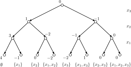
Figure 2: The Fourier coefficients of the restricted versions of $p$ from Example 1. Depth 0 (root) corresponds to the Fourier transform of $p\downarrow_{2^{\emptyset}}$, depth 1 to the one of $p\downarrow_{2^{\{x_{3}\}}}$, depth 2 to the one of $p\downarrow_{2^{\{x_{2},x_{3}\}}}$ and depth 3 to the one of $p$.

Algorithm. We initialize SSFT with $M_{0}=\emptyset$ and ${s\downarrow_{2^{\emptyset}}\left(\emptyset\right)}=s\left(\emptyset\right)$ (lines 1–2). Then, in each iteration of the for loop (line 3), we grow our set $M_{i}=M_{i-1}\cup\{x_{i}\}$ by adding the next element (line 4), determine the superset $\mathcal{B}$ of $\operatorname{supp}(\savestack{\tmpbox}{\stretchto{\scaleto{\scalerel*[\widthof{s\downarrow_{2^{M_{i}}}}]{\kern-0.6pt\bigwedge\kern-0.6pt}{\rule[-650.43pt]{4.30554pt}{650.43pt}}}{}}{0.5ex}}\stackon[1pt]{s\downarrow_{2^{M_{i}}}}{\tmpbox})$ based on the Fourier coefficients from the previous iteration $\savestack{\tmpbox}{\stretchto{\scaleto{\scalerel*[\widthof{s\downarrow_{2^{M_{i-1}}}}]{\kern-0.6pt\bigwedge\kern-0.6pt}{\rule[-650.43pt]{4.30554pt}{650.43pt}}}{}}{0.5ex}}\stackon[1pt]{s\downarrow_{2^{M_{i-1}}}}{\tmpbox}$ (lines 5–8) and solve the resulting known-support-problem using Theorem 1 (lines 9–12). After $n$ iterations we end up with the Fourier coefficients of $s$.

We depict an execution of SSFT on $p$ from Example 1 in Fig. 2. We process the elements $x_{1},x_{2},x_{3}$ in reverse order, which results in the final Fourier coefficients being lexicographically ordered. Note that in this example applying SSFT naively would fail, as $\savestack{\tmpbox}{\stretchto{\scaleto{\scalerel*[\widthof{p\downarrow_{2^{\emptyset}}}]{\kern-0.6pt\bigwedge\kern-0.6pt}{\rule[-650.43pt]{4.30554pt}{650.43pt}}}{}}{0.5ex}}\stackon[1pt]{p\downarrow_{2^{\emptyset}}}{\tmpbox}\left(\emptyset\right)=p\left(\emptyset\right)=0$ SSFT would falsely conclude that both $\savestack{\tmpbox}{\stretchto{\scaleto{\scalerel*[\widthof{p\downarrow_{2^{\{x_{3}\}}}}]{\kern-0.6pt\bigwedge\kern-0.6pt}{\rule[-650.43pt]{4.30554pt}{650.43pt}}}{}}{0.5ex}}\stackon[1pt]{p\downarrow_{2^{\{x_{3}\}}}}{\tmpbox}\left(\emptyset\right)$ and $\savestack{\tmpbox}{\stretchto{\scaleto{\scalerel*[\widthof{p\downarrow_{2^{\{x_{3}\}}}}]{\kern-0.6pt\bigwedge\kern-0.6pt}{\rule[-650.43pt]{4.30554pt}{650.43pt}}}{}}{0.5ex}}\stackon[1pt]{p\downarrow_{2^{\{x_{3}\}}}}{\tmpbox}\left(\{x_{3}\}\right)$ are zero resulting in them and their children being pruned. Instead, we initialize the algorithm with $\savestack{\tmpbox}{\stretchto{\scaleto{\scalerel*[\widthof{p\downarrow_{\{x_{3}\}}}]{\kern-0.6pt\bigwedge\kern-0.6pt}{\rule[-650.43pt]{4.30554pt}{650.43pt}}}{}}{0.5ex}}\stackon[1pt]{p\downarrow_{\{x_{3}\}}}{\tmpbox}$. The levels of the tree correspond to the elements of the chain (18). When computing the Fourier coefficients of a level, the ones of the previous level determine the support superset $\mathcal{B}$. Whenever, SSFT encounters a Fourier coefficient that is equal to zero, all of its children are pruned from the tree. For example, $\savestack{\tmpbox}{\stretchto{\scaleto{\scalerel*[\widthof{p\downarrow_{2^{\{x_{2},x_{3}\}}}}]{\kern-0.6pt\bigwedge\kern-0.6pt}{\rule[-650.43pt]{4.30554pt}{650.43pt}}}{}}{0.5ex}}\stackon[1pt]{p\downarrow_{2^{\{x_{2},x_{3}\}}}}{\tmpbox}\left(\{x_{2},x_{3}\}\right)=0$, thus, $\{x_{2},x_{3}\}$ and $\{x_{1},x_{2},x_{3}\}$ are not included in the support superset $\mathcal{B}$ of $\savestack{\tmpbox}{\stretchto{\scaleto{\scalerel*[\widthof{p\downarrow_{N}}]{\kern-0.6pt\bigwedge\kern-0.6pt}{\rule[-650.43pt]{4.30554pt}{650.43pt}}}{}}{0.5ex}}\stackon[1pt]{p\downarrow_{N}}{\tmpbox}=\widehat{p}$. While pruning in our small example only avoids the computation of $\savestack{\tmpbox}{\stretchto{\scaleto{\scalerel*[\widthof{p\downarrow_{2^{N}}}]{\kern-0.6pt\bigwedge\kern-0.6pt}{\rule[-650.43pt]{4.30554pt}{650.43pt}}}{}}{0.5ex}}\stackon[1pt]{p\downarrow_{2^{N}}}{\tmpbox}\left(\{x_{2},x_{3}\}\right)$ and $\savestack{\tmpbox}{\stretchto{\scaleto{\scalerel*[\widthof{p\downarrow_{2^{N}}}]{\kern-0.6pt\bigwedge\kern-0.6pt}{\rule[-650.43pt]{4.30554pt}{650.43pt}}}{}}{0.5ex}}\stackon[1pt]{p\downarrow_{2^{N}}}{\tmpbox}\left(\{x_{1},x_{2},x_{3}\}\right)$, it avoids an exponential amount of computation in larger examples (for $|N|=n$, when $\savestack{\tmpbox}{\stretchto{\scaleto{\scalerel*[\widthof{s\downarrow_{2^{M_{i-1}}}}]{\kern-0.6pt\bigwedge\kern-0.6pt}{\rule[-650.43pt]{4.30554pt}{650.43pt}}}{}}{0.5ex}}\stackon[1pt]{s\downarrow_{2^{M_{i-1}}}}{\tmpbox}\left(B\right)=0$ the two subtrees of height $n-i$ containing its children are pruned).

Note that for practical reasons we only process up to $k_{\text{max}}$ subsets in line 6. In line 11, we consider a Fourier coefficient $|\mathbf{x}_{B}|<\epsilon$ (a hyperparameter) as zero.

Analysis. We consider set functions $s$ that are $k$-Fourier-sparse (but not $(k-1)$-Fourier-sparse) with support $\operatorname{supp}(\widehat{s})=\{B_{1},\dots,B_{k}\}=\mathcal{B}$, i.e., $\{{s:2^{N}\to\mathbb{R}}:{\widehat{s}\left(B\right)\neq 0}\text{ iff }B\in\mathcal{B}\}$, which is isomorphic to

$$\mathcal{S}=\{\widehat{\mathbf{s}}\in\mathbb{R}^{k}:\widehat{\mathbf{s}}_{i}\neq 0\text{ for all }i\in\{1,\dots,k\}\}.$$ (19)

Let $\lambda$ denote the Lebesgue measure on $\mathbb{R}^{k}$. Let $\mathcal{P}^{M_{i}}_{C}=\{B\in\mathcal{B}:B\cap M_{i}=C\}$.

Pathological set functions. SSFT fails to compute the Fourier coefficients for which $\savestack{\tmpbox}{\stretchto{\scaleto{\scalerel*[\widthof{s\downarrow_{2^{M_{i}}}}]{\kern-0.6pt\bigwedge\kern-0.6pt}{\rule[-650.43pt]{4.30554pt}{650.43pt}}}{}}{0.5ex}}\stackon[1pt]{s\downarrow_{2^{M_{i}}}}{\tmpbox}\left(C\right)=0$ despite $\mathcal{P}^{M_{i}}_{C}\neq\emptyset$. Thus, the set of pathological set functions $\mathcal{D}_{1}$, i.e., the set of set functions for which SSFT fails, can be written as the finite union of kernels

$$\mathcal{K}_{1}(M_{i},C)=\{\widehat{\mathbf{s}}\in\mathbb{R}^{k}:\savestack{\tmpbox}{\stretchto{\scaleto{\scalerel*[\widthof{s\downarrow_{2^{M_{i}}}}]{\kern-0.6pt\bigwedge\kern-0.6pt}{\rule[-650.43pt]{4.30554pt}{650.43pt}}}{}}{0.5ex}}\stackon[1pt]{s\downarrow_{2^{M_{i}}}}{\tmpbox}\left(C\right)=0\}$$ (20)

intersected with $\mathcal{S}$.

Theorem 2.

Using prior notation, the set of pathological set functions for SSFT is given by

$$\mathcal{D}_{1}=\bigcup_{i=0}^{n-1}\bigcup_{C\subseteq M_{i}:\mathcal{P}^{M_{i}}_{C}\neq\emptyset}\mathcal{K}_{1}(M_{i},C)\cap\mathcal{S},$$ (21)

and has Lebesgue measure zero, i.e., $\lambda(\mathcal{D}_{1})=0$.

Complexity. By reusing queries and computations from the $(i-1)$-th iteration of SSFT in the $i$-th iteration, we obtain:

Theorem 3.

SSFT requires at most ${nk-k\log_{2}k+k}$ queries and $O(nk^{2})$ operations.

3.3 Shrinking the Set of Pathological Fourier Coefficients

According to Theorem 2, the set of pathological Fourier coefficients for a given support has measure zero. However, unfortunately, this set includes important classes of set functions including graph cuts (in the case of unit weights) and hypergraph cuts.

Solution. The key idea to exclude these and further narrow down the set of pathological cases is to use the convolution theorem (6), i.e., the fact that we can modulate Fourier coefficients by filtering. Concretely, we choose a random filter $h$ such that SSFT works for $h*s$ with probability one. $\widehat{s}$ is then obtained from $\widehat{h*s}$ by dividing by the frequency response $\overline{h}$. We keep the associated overhead in $O(n)$ by choosing a one-hop filter, i.e., $h(B)=0$ for $|B|>1$. Motivated by the fact that, e.g., the product of a Rademacher random variable (which would lead to cancellations) and a normally distributed random variable is again normally distributed, we sample our filtering coefficients i.i.d. from a normal distribution. By filtering our signal with such a random filter we aim to end up in a situation similar to Lemma 6. We call the resulting algorithm SSFT+, shown above.

Algorithm. In SSFT+ we create a random one-hop filter $h$ (lines 2–4), apply SSFT to the filtered signal $h*s$ (line 6) and compute $\widehat{s}$ based on $\widehat{h*s}$ (lines 8–9).

Analysis. Building on the analysis of SSFT, recall that $\mathcal{S}$ denotes the set of $k$-Fourier-sparse (but not $(k-1)$-Fourier-sparse) set functions and $\mathcal{P}_{C}^{M_{i}}$ are the elements $B\in\operatorname{supp}(\widehat{s})$ satisfying $B\cap M_{i}=C$. Let

$$\mathcal{K}_{2}(M_{i},C)=\left\{\widehat{\mathbf{s}}\in\mathbb{R}^{k}:\savestack{\tmpbox}{\stretchto{\scaleto{\scalerel*[\widthof{s\downarrow_{2^{M_{i}}}}]{\kern-0.6pt\bigwedge\kern-0.6pt}{\rule[-650.43pt]{4.30554pt}{650.43pt}}}{}}{0.5ex}}\stackon[1pt]{s\downarrow_{2^{M_{i}}}}{\tmpbox}\left(C\right)=0\text{ and }\right.\\ \left.\savestack{\tmpbox}{\stretchto{\scaleto{\scalerel*[\widthof{s\downarrow_{2^{M_{i}\cup\{x_{j}\}}}}]{\kern-0.6pt\bigwedge\kern-0.6pt}{\rule[-650.43pt]{4.30554pt}{650.43pt}}}{}}{0.5ex}}\stackon[1pt]{s\downarrow_{2^{M_{i}\cup\{x_{j}\}}}}{\tmpbox}\left(C\right)=0\text{ for }j\in\{i+1,\dots,n\}\right\}.$$ (22)

Theorem 4.

With probability one with respect to the randomness of the filtering coefficients, the set of pathological set functions for SSFT+ has the form (using prior notation)

$$\mathcal{D}_{2}=\bigcup_{i=0}^{n-2}\bigcup_{C\subseteq M_{i}:\mathcal{P}^{M_{i}}_{C}\neq\emptyset}\mathcal{K}_{2}(M_{i},C)\cap\mathcal{S}.$$ (23)

Theorem 4 shows that SSFT+ correctly processes $\savestack{\tmpbox}{\stretchto{\scaleto{\scalerel*[\widthof{s\downarrow_{2^{M_{i}}}}]{\kern-0.6pt\bigwedge\kern-0.6pt}{\rule[-650.43pt]{4.30554pt}{650.43pt}}}{}}{0.5ex}}\stackon[1pt]{s\downarrow_{2^{M_{i}}}}{\tmpbox}\left(C\right)=0$ with $\mathcal{P}^{M_{i}}_{C}\neq\emptyset$, iff there is an element $x\in\{x_{i+1},\dots,x_{n}\}$ for which $\savestack{\tmpbox}{\stretchto{\scaleto{\scalerel*[\widthof{s\downarrow_{2^{M_{i}\cup\{x\}}}}]{\kern-0.6pt\bigwedge\kern-0.6pt}{\rule[-650.43pt]{4.30554pt}{650.43pt}}}{}}{0.5ex}}\stackon[1pt]{s\downarrow_{2^{M_{i}\cup\{x\}}}}{\tmpbox}\left(C\right)\neq 0$.

Theorem 5.

If $\mathcal{D}_{1}$ is non-empty, $\mathcal{D}_{2}$ is a proper subset of $\mathcal{D}_{1}$. In particular, $\mathcal{K}_{1}(M_{i},C)\cap S\neq\emptyset$ implies $\mathcal{K}_{2}(M_{i},C)<_{\mathbb{R}}\mathcal{K}_{1}(M_{i},C)$, for all $C\subseteq M_{i}\subseteq N$ with $\mathcal{P}_{C}^{M_{i}}\neq\emptyset$.

Complexity. There is a trade-off between the number of non-zero filtering coefficients and the size of the set of pathological set functions. For example, for the one-hop filters used, computing $(h*s)\left(A\right)$ requires $1+n-|A|$ queries.

Theorem 6.

The query complexity of SSFT+ is $O(n^{2}k-nk\log k)$ and the algorithmic complexity is $O(n^{2}k+nk^{2})$.

4 Related Work

We briefly discuss related work on learning set functions.

Fourier-sparse learning. There is a substantial body of research concerned with learning Fourier/WHT-sparse set functions (Stobbe and Krause 2012; Scheibler, Haghighatshoar, and Vetterli 2013; Kocaoglu et al. 2014; Li and Ramchandran 2015; Cheraghchi and Indyk 2017; Amrollahi et al. 2019). Recently, Amrollahi et al. (2019) have imported ideas from the hashing based sparse Fourier transform algorithm (Hassanieh et al. 2012) to the set function setting. The resulting algorithms compute the WHT of $k$-WHT-sparse set functions with a query complexity $O(nk)$ for general frequencies, $O(kd\log n)$ for low degree ($\leq d$) frequencies and $O(kd\log n\log(d\log n))$ for low degree set functions that are only approximately sparse. To the best of our knowledge this latest work improves on previous algorithms, such as the ones by Scheibler, Haghighatshoar, and Vetterli (2013), Kocaoglu et al. (2014), Li and Ramchandran (2015), and Cheraghchi and Indyk (2017), providing the best guarantees in terms of both query complexity and runtime. E.g., Scheibler, Haghighatshoar, and Vetterli (2013) utilize similar ideas like hashing/aliasing to derive sparse WHT algorithms that work under random support (the frequencies are uniformly distributed on $2^{N}$) and random coefficient (the coefficients are samples from continuous distributions) assumptions. Kocaoglu et al. (2014) propose a method to compute the WHT of a $k$-Fourier-sparse set function that satisfies a so-called unique sign property using queries polynomial in $n$ and $2^{k}$.

In a different line of work, Stobbe and Krause (2012) utilize results from compressive sensing to compute the WHT of $k$-WHT-sparse set functions, for which a superset $\mathcal{P}$ of the support is known. This approach also can be used to find a $k$-Fourier-sparse approximation and has a theoretical query complexity of $O(k\log^{4}|\mathcal{P}|)$. In practice, it even seems to be more query-efficient than the hashing based WHT (see experimental section of Amrollahi et al. (2019)), but suffers from the high computational complexity, which scales at least linearly with $|\mathcal{P}|$. Regrading coverage functions, to our knowledge, there has not been any work in the compressive sensing literature for the non-orthogonal Fourier bases which do not satisfy RIP properties and hence lack sparse recovery and robustness guarantees.

In summary, all prior work on Fourier-based methods for learning set functions was based on the WHT. Our work leverages the broader framework of signal processing with set functions proposed by Püschel and Wendler (2020), which provides a larger class of Fourier transforms and thus new types of Fourier-sparsity.

Other learning paradigms. Other lines of work for learning set functions include methods based on new neural architectures (Dolhansky and Bilmes 2016; Zaheer et al. 2017; Weiss, Lubin, and Seuken 2017), methods based on backpropagation through combinatorial solvers (Djolonga and Krause 2017; Tschiatschek, Sahin, and Krause 2018; Wang et al. 2019; Vlastelica et al. 2019), kernel based methods (Buathong, Ginsbourger, and Krityakierne 2020), and methods based on other succinct representations such as decision trees (Feldman, Kothari, and Vondrák 2013) and disjunctive normal forms (Raskhodnikova and Yaroslavtsev 2013).

5 Empirical Evaluation

We evaluate the two variants of our algorithm (SSFT and SSFT+) for model 4 on three classes of real-world set functions. First, we approximate the objective functions of sensor placement tasks by Fourier-sparse functions and evaluate the quality of the resulting surrogate objective functions. Second, we learn facility locations functions (which are preference functions) that are used to determine cost-effective sensor placements in water networks (Leskovec et al. 2007). Finally, we learn simulated bidders from a spectrum auctions test suite (Weiss, Lubin, and Seuken 2017).

Benchmark learning algorithms. We compare our algorithm against three state-of-the-art algorithms for learning WHT-sparse set functions: the compressive sensing based approach CS-WHT (Stobbe and Krause 2012), the hashing based approach H-WHT (Amrollahi et al. 2019), and the robust version of the hashing based approach R-WHT (Amrollahi et al. 2019). For our algorithm we set $\epsilon=0.001$ and $k_{\text{max}}=1000$. CS-WHT requires a superset $\mathcal{P}$ of the (unknown) Fourier support, which we set to all $B\subseteq N$ with $|B|\leq 2$ and the parameter for expected sparsity to $1000$. For H-WHT we used the exact algorithm without low-degree assumption and set the expected sparsity parameter to $2000$. For R-WHT we used the robust algorithm without low-degree assumption and set the expected sparsity parameter to $2000$ unless specified otherwise.

5.1 Sensor Placement Tasks

We consider a discrete set of sensors located at different fixed positions measuring a quantity of interest, e.g., temperature, amount of rainfall, or traffic data, and want to find an informative subset of sensors subject to a budget constraint on the number of sensors selected (e.g., due to hardware costs). To quantify the informativeness of subsets of sensors, we fit a multivariate normal distribution to the sensor measurements (Krause, Singh, and Guestrin 2008) and associate each subset of sensors $A\subseteq N$ with its information gain (Srinivas et al. 2010)

$$G\left(A\right)=\frac{1}{2}\log|I_{|A|}+\sigma^{-2}(K_{ij})_{i,j\in A}|,$$ (24)

where $(K_{ij})_{i,j\in A}$ is the submatrix of the covariance matrix $K$ that is indexed by the sensors $A\subseteq N$ and $I_{|A|}$ the $|A|\times|A|$ identity matrix. We construct two covariance matrices this way for temperature measurements from 46 sensors at Intel Research Berkeley and for velocity data from 357 sensors deployed under a highway in California.

The information gain is a submodular set function and, thus, can be approximately maximized using the greedy algorithm by Nemhauser, Wolsey, and Fisher (1978): $A^{*}\approx\operatorname*{arg\,max}_{A\subseteq N:|A|\leq d}G\left(A\right)$ to obtain informative subsets. We do the same using Fourier-sparse surrogates $s$ of $G$: $A^{+}\approx\operatorname*{arg\,max}_{A\subseteq N:|A|\leq d}s\left(A\right)$ and compute $G(A^{+})$. As a baseline we place $d$ sensors at random $A_{\text{rand}}$ and compute $G\left(A_{\text{rand}}\right)$. Figure 3 shows our results. The x-axes correspond to the cardinality constraint used during maximization and the y-axes to the information gain obtained by the respective informative subsets. In addition, we report next to the legend the execution time and number of queries needed by the successful experiments.

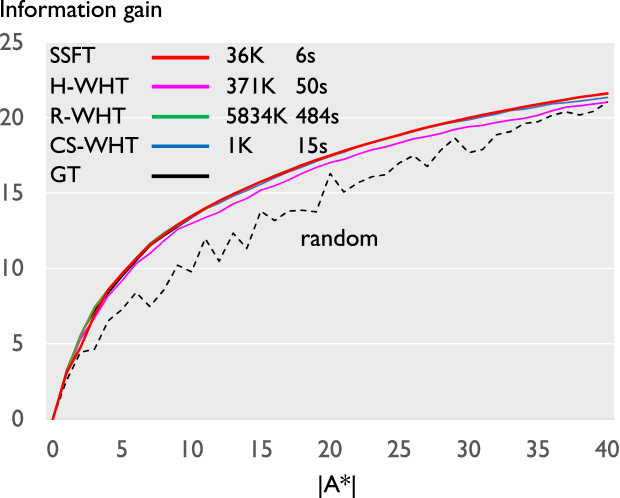
(a) Berkeley, $n=46$

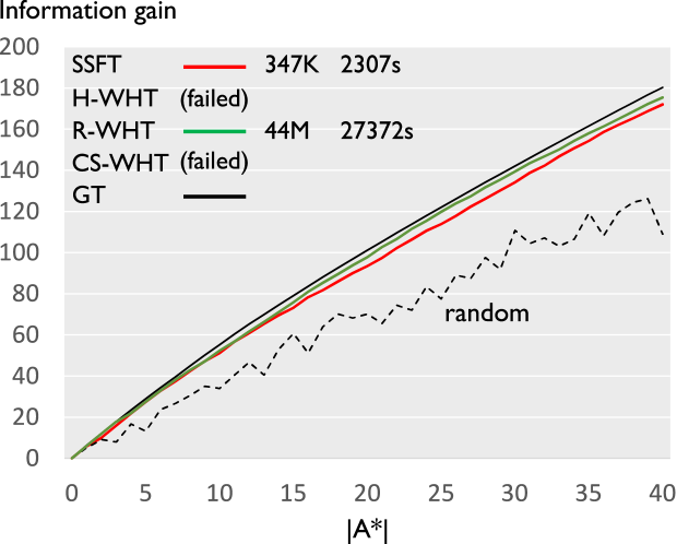
(b) California, $n=357$

Figure 3: Comparison of learnt surrogate objective functions on submodular maximization tasks subject to cardinality constraints (x-axis); On the y-axis we plot the information gain achieved by the informative subset obtained by the respective method. We report the number of queries and execution time in seconds next to the legend or indicate failure.

Interpretation of results. H-WHT only works for the Berkeley data. For the other data set it is not able to reconstruct enough Fourier coefficients to provide a meaningful result. The likely reason is that the target set function is not exactly Fourier-sparse, which can cause an excessive amount of collisions in the hashing step. In contrast, CS-WHT is noise-robust and yields sensor placements that are indistinguishable from the ones obtained by maximizing the true objective function in the first task. However, for the California data, CS-WHT times out. In contrast, SSFT and R-WHT work well on both tasks. In the first task, SSFT is on par with CS-WHT in terms of sensor placement quality and significantly faster despite requiring more queries. On the California data, SSFT yields sensor placements of similar quality as the ones obtained by R-WHT while requiring orders of magnitude fewer queries and time.

5.2 Learning Preference Functions

We now consider a class of preference functions that are used for the cost-effective contamination detection in water networks (Leskovec et al. 2007). The networks stem from the Battle of Water Sensor Networks (BSWN) challenge (Ostfeld et al. 2008). The junctions and pipes of each BSWN network define a graph. Additionally, each BSWN network has dynamic parameters such as time-varying water consumption demand patterns, opening and closing valves, and so on.

To determine a cost-effective subset of sensors (e.g., given a maximum budget), Leskovec et al. (2007) make use of facility locations functions of the form

$$p:2^{N}\to\mathbb{R};A\mapsto\sum_{\ell=1}^{L}\max_{i\in A}r_{\ell i},$$ (25)

where $r$ is a matrix in $\mathbb{R}_{\geq 0}^{L\times n}$. Each row corresponds to an event (e.g., contamination of the water network at any junction) and the entry $r_{\ell i}$ quantifies the utility of the $i$-th sensor in case of the $\ell$-th event. It is straightforward to see that (25) is a preference function with $a=0$ and $u_{i}=\sum_{\ell=1}^{L}r_{\ell i}$. Thus, they are sparse w.r.t. model 4 and dense w.r.t. WHT (see Lemma 1).

Leskovec et al. (2007) determined three different utility matrices $r\in\mathbb{R}^{3424\times 12527}$ that take into account the fraction of events detected, the detection time, and the population affected, respectively. The matrices were obtained by costly simulating millions of possible contamination events in a 48 hour timeframe. For our experiments we select one of the utility matrices and obtain subnetworks by selecting the columns that provide the maximum utility, i.e., we select the $|N|=n$ columns $j$ with the largest $\max_{\ell}r_{\ell j}$.

Table 2: Comparison of model 4 sparsity (SSFT) against WHT sparsity (R-WHT) of facility locations functions in terms of reconstruction error $\|\mathbf{p}-\mathbf{p^{\prime}}\|/\|\mathbf{p}\|$ for varying $|N|$; The italic results are averages over 10 runs.

$|N|$		$\alpha$	queries	time (s)	$k$	$\|\mathbf{p}-\mathbf{p^{\prime}}\|/\|\mathbf{p}\|$
$20$	SSFT		$734$	$0.12$	$102$	$\mathrm{𝟎}$
	WHT				$2^{9}$	$0.000143$
					$2^{14}$	$0.000078$
					$2^{19}$	$0.000001$
$50$	SSFT		$10K$	$2$	$648$	$\mathrm{𝟎}$
	R-WHT	1	$\mathit{2,103K}$	$\mathit{361}$	$\mathit{1,380}$	$\mathit{0.001744}$
		2	$\mathit{4,192K}$	$\mathit{766}$	$\mathit{2,739}$	$\mathit{0.000847}$
		4	$\mathit{8,370K}$	$\mathit{1,499}$	$\mathit{5,054}$	$\mathit{0.000129}$
		8	$\mathit{16,742K}$	$\mathit{2,838}$	$\mathit{9,547}$	$\mathit{0.000108}$
$100$	SSFT		$76K$	$24$	$2,308$	$\mathrm{𝟎}$
	R-WHT	1	$16,544K$	$5,014$	$2,997$	$0.000546$
		2	$33,100K$	$10,265$	$6,466$	$0.000380$
$200$	SSFT		$494K$	$451$	$7,038$	$\mathrm{𝟎}$
$300$	SSFT		$1,644K$	$2,368$	$16,979$	$\mathrm{𝟎}$
$400$	SSFT		$3,859K$	$7,654$	$28,121$	$\mathrm{𝟎}$
$500$	SSFT		$7,218K$	$17,693$	$38,471$	$\mathrm{𝟎}$

Table 3: Multi-region valuation model ($n=98$). Each row corresponds to a different bidder type.

	number of queries (in thousands)			Fourier coefficients recovered			relative reconstruction error
B. type	SSFT	SSFT+	H-WHT	SSFT	SSFT+	H-WHT	SSFT	SSFT+	H-WHT
local	$3\pm 4$	$229\pm 73$	$781\pm 0$	$118\pm 140$	$303\pm 93$	$675\pm 189$	$0.5657\pm 0.4900$	$0\pm 0$	$0\pm 0$
regional	$20\pm 1$	$646\pm 12$	$781\pm 0$	$659\pm 32$	$813\pm 36$	$1,779\pm 0$	$0.0118\pm 0.0071$	$0\pm 0$	$0\pm 0$
national	$71\pm 0$	$3,305\pm 1$	$781\pm 0$	$1,028\pm 3$	$1,027\pm 6$	$4,170\pm 136$	$0.0123\pm 0.0014$	$0.0149\pm 0.0089$	$0.2681\pm 0.2116$

In Table 2 we compare the sparsity of the corresponding facility locations function in model 4 against its sparsity in the WHT. For $|N|=20$, we compute the full WHT and select the $k$ largest coefficients. For $|N|>20$, we compute the $k$ largest WHT coefficients using R-WHT. The model 4 coefficients are always computed using SSFT. If the facility locations function is $k$ sparse w.r.t. model 4 for some $|N|=n$, we set the expected sparsity parameter of R-WHT to different multiples $\alpha k$ up to the first $\alpha$ for which the algorithm runs out of memory. We report the number of queries, time, number of Fourier coefficients $k$, and relative reconstruction error. For R-WHT experiments that require less than one hour we report average results over 10 runs (indicated by italic font). For $|N|>20$, the relative error cannot be computed exactly and thus is obtained by sampling 100,000 sets $\mathcal{A}$ uniformly at random and computing $\|\mathbf{p}_{\mathcal{A}}-\mathbf{p^{\prime}}_{\mathcal{A}}\|/\|\mathbf{p}_{\mathcal{A}}\|$, where $p$ denotes the real facility locations function and $p^{\prime}$ the estimate.

Interpretation of results. The considered facility locations functions are indeed sparse w.r.t. model 4 and dense w.r.t. the WHT. As expected, SSFT outperforms R-WHT in this scenario, which can be seen by the lower number of queries, reduced time, and an error of exactly zero for the SSFT. This experiment shows certain classes of set functions of practical relevance are better represented in the model 4 basis than in the WHT basis.

5.3 Preference Elicitation in Auctions

In combinatorial auctions a set of goods $N=\{x_{1},\dots,x_{n}\}$ is auctioned to a set of $m$ bidders. Each bidder $j$ is modeled as a set function $b_{j}:2^{N}\to\mathbb{R}$ that maps each bundle of goods to its subjective value for this bidder. The problem of learning bidder valuation functions from queries is known as the preference elicitation problem (Brero, Lubin, and Seuken 2019). Our experiment sketches an approach under the assumption of Fourier sparsity.

As common in this field (Weissteiner and Seuken 2020; Weissteiner et al. 2020), we resort to simulated bidders. Specifically, we use the multi-region valuation model (MRVM) from the spectrum auctions test suite (Weiss, Lubin, and Seuken 2017). In MRVM, 98 goods are auctioned off to 10 bidders of different types (3 local, 4 regional, and 3 national). We learn these bidders using the prior Fourier-sparse learning algorithms, this time including SSFT+, but excluding CS-WHT, since $\mathcal{P}$ is not known in this scenario. Table 3 shows the results: means and standard deviations of the number of queries required, Fourier coefficients recovered, and relative error (estimated using 10,000 samples) taken over the bidder types and 25 runs.

Interpretation of results. First, we note that SSFT+ can indeed improve over SSFT for set functions that are relevant in practice. Namely, SSFT+ consistently learns sparse representations for local and regional bidders, while SSFT fails. H-WHT also achieves perfect reconstruction for local and regional bidders. For the remaining bidders none of the methods achieves perfect reconstruction, which indicates that those bidders do not admit a sparse representation. Second, we observe that, for the local and regional bidders, in the non-orthogonal model 4 basis only half as many coefficients are required as in the WHT basis. Third, SSFT+ requires less queries than H-WHT in the Fourier-sparse cases.

6 Conclusion

We introduced an algorithm for learning set functions that are sparse with respect to various generalized, non-orthogonal Fourier bases. In doing so, our work significantly expands the set of efficiently learnable set functions. As we explained, the new notions of sparsity connect well with preference functions in recommender systems and the notions of complementarity and substitutability, which we consider an exciting avenue for future research.

Ethics Statement

Our approach is motivated by a range of real world applications, including modeling preferences in recommender systems and combinatorial auctions, that require the modeling, processing, and analysis of set functions, which is notoriously difficult due to their exponential size. Our work adds to the tool set that makes working with set functions computationally tractable. Since the work is of foundational and algorithmic nature we do not see any immediate ethical concerns. In case that the models estimated with our algorithms are used for making decisions (such as recommendations, or allocations in combinatorial auctions), of course additional care has to be taken to ensure that ethical requirements such as fairness are met. These questions are complementary to our work.

Appendix

Appendix A Preference Functions

Table 4: Shifts and Fourier concepts.

$\begin{array}[]{@{}l llllll@{}}\hline\cr\hline\cr\text{model }&\text{shift }T_{Q}s\left(A\right)&B\text{-th basis vec. }\mathbf{f}^{B}_{A}=&F\text{ (sum)}:\widehat{s}\left(B\right)=&F^{-1}\text{ (sum)}:{s}_{A}=&\text{known as}\\ \hline\cr 3&s\left(A\setminus Q\right)&(-1)^{|B|}\iota_{B\subseteq A}&\displaystyle\sum_{\stackrel{{\scriptstyle A\subseteq B}}{{\hphantom{A\cup B=N}}}}(-1)^{|A|}s\left(A\right)&\hphantom{\tfrac{1}{2^{n}}}\displaystyle\sum_{\stackrel{{\scriptstyle B\subseteq A}}{{\hphantom{A\cap B=\emptyset}}}}(-1)^{|B|}\widehat{s}\left(B\right)&\text{Zeta transform \cite[citep]{(\@@bibref{AuthorsPhrase1Year}{bjorklund2007fourier}{\@@citephrase{{} }}{})}}\\[14.22636pt] 4&s\left(A\cup Q\right)&\iota_{A\cap B=\emptyset}&\displaystyle\sum_{\stackrel{{\scriptstyle A\subseteq N:}}{{A\cup B=N}}}(-1)^{|A\cap B|}s\left(A\right)&\hphantom{\tfrac{1}{2^{n}}}\displaystyle\sum_{\stackrel{{\scriptstyle B\subseteq N:}}{{A\cap B=\emptyset}}}\widehat{s}\left(B\right)&\text{W-transform \cite[citep]{(\@@bibref{AuthorsPhrase1Year}{chakrabarty2012testing}{\@@citephrase{{} }}{})}}\\[14.22636pt] 5&s\left(A\setminus Q\cup Q\setminus A\right)&\tfrac{1}{2^{n}}(-1)^{|A\cap B|}&\displaystyle\sum_{\stackrel{{\scriptstyle A\subseteq N}}{{\hphantom{A\cup B=N}}}}(-1)^{|A\cap B|}s\left(A\right)&\tfrac{1}{2^{n}}\displaystyle\sum_{\stackrel{{\scriptstyle B\subseteq N}}{{\hphantom{A\cap B=\emptyset}}}}(-1)^{|A\cap B|}\widehat{s}\left(B\right)&\text{WHT \cite[citep]{(\@@bibref{AuthorsPhrase1Year}{bernasconi1996fourier}{\@@citephrase{{} }}{})}}\\ \hline\cr\hline\cr\end{array}$

Let $N=\{x_{1},\dots,x_{n}\}$ denote our ground set. For this section, we assume $x_{1}=1,\dots,x_{n}=n$.

An important aspect of our work is that certain set functions are sparse in one basis but not in the others. In this section we show that preference functions (Djolonga, Tschiatschek, and Krause 2016) indeed constitute a class of set functions that are sparse w.r.t. model 4 (see Table 4, which we replicate from the paper for convenience) and dense w.r.t. model 5 (= WHT basis). Preference functions naturally occur in machine learning tasks on discrete domains such as recommender systems and auctions, in which they, e.g., are used to model complementary- and substitution effects between goods. Goods complement each other when their combined utility is greater than the sum of their individual utilities. E.g., a pair of shoes is more useful than the two shoes individually and a round trip has higher utility than the combined individual utilities of outward and inward flight. Analogously, goods substitute each other when their combined utility is smaller than the sum of their individual utilities. E.g., it might not be necessary to buy a pair of glasses if you already have one. Formally, a preference function is given by

$$p:2^{N}\to\mathbb{R};A\mapsto\sum_{i\in A}u_{i}+\sum_{\ell=1}^{L}\left(\max_{i\in A}r_{\ell i}-\sum_{i\in A}r_{\ell i}\right)$$ (26)

$$-\sum_{k=1}^{K}\left(\max_{i\in A}a_{ki}-\sum_{i\in A}a_{ki}\right).$$

Equation (26) is composed of a modular part parametrized by $u\in\mathbb{R}^{n}$, a repulsive part parametrized by $r\in\mathbb{R}_{\geq 0}^{L\times n}$, with ${L\in\mathbb{N}}$, and an attractive part parametrized by $a\in\mathbb{R}_{\geq 0}^{K\times n}$, with $K\in\mathbb{N}$.

Lemma 3.

Preference functions of the form (26) are Fourier-sparse w.r.t. model 4.

Proof.

In order to prove that preference functions are sparse w.r.t. model 4 we exploit the linearity of the Fourier transform. That is, we are going to show that $p$ is Fourier sparse by showing that it is a sum of Fourier sparse set functions. In particular, there are only two types of summands (= set functions):

First, $A\mapsto\sum_{i\in A}u_{i}$, $A\mapsto-\sum_{i\in A}r_{\ell i}$, for $\ell\in\{1,\dots,L\}$, and $A\mapsto\sum_{i\in A}a_{ki}$, for $k\in\{1,\dots,K\}$, are modular set functions whose only non-zero Fourier coefficients are summed up in $\widehat{p}\left(\{x\}\right)$ for $x\in N$ and $\widehat{p}\left(\emptyset\right)$.

Second, $f_{\ell}(A)=\max_{i\in A}r_{{\ell}i}$, for $\ell\in\{1,\dots,L\}$, and $g_{k}(A)=-\max_{i\in A}a_{ki}$, for $k\in\{1,\dots,K\}$, are weighted- and negative weighted coverage functions, respectively. In order to see that ${f_{\ell}\left(A\right)=\max_{i\in A}r_{{\ell}i}}$ is a weighted coverage function, observe that the codomain of $f_{\ell}$ is $\{r_{{\ell}1},\dots,r_{{\ell}n}\}$. Let $\sigma:N\to N$ denote the permutation that sorts $r_{\ell}$, i.e., $r_{{\ell}\sigma(1)}<r_{{\ell}\sigma(2)}<\cdots<r_{{\ell}\sigma(n)}$. Let $U=\{1,\dots,n\}$ denote the universe. We set ${w(u)=r_{{\ell}\sigma(u)}-r_{{\ell}\sigma(u-1)}}$ for $u\geq 2$ and ${w(u)=r_{{\ell}\sigma(1)}}$ for $u=1$. Let $M=\{S_{1},\dots,S_{n}\}$. Let the set $S_{i}=\{1,\dots,\sigma^{-1}(i)\}$. In words, $S_{i}$ covers all elements $u$ that correspond to smaller values $r_{\ell\sigma(u)}$, i.e., $u$ with $r_{\ell\sigma(u)}\leq r_{\ell i}$. By construction of $w(u)$ we have $\mathbf{w}(S_{i})=r_{\ell\sigma(1)}+(r_{\ell\sigma(2)}-r_{\ell\sigma(1)})+\dots+(r_{\ell\sigma(\sigma^{-1}(i))}-r_{\ell\sigma(\sigma^{-1}(i)-1)})=r_{\ell i}$, and, because of $S_{\sigma(1)}\subset S_{\sigma(2)}\subset\cdots\subset S_{\sigma(n)}$ we have, for all $A\subseteq N$,

$$\mathbf{w}\left(\bigcup_{i\in A}S_{i}\right)=\mathbf{w}(S_{j})=r_{\ell j},$$ (27)

where $j$ is the element in $A$ that satisfies $S_{i}\subseteq S_{j}$ for all $i\in A$. Now, observe that $S_{i}\subseteq S_{j}$ is equivalent to $r_{\ell i}\leq r_{\ell j}$. Thus, by definition of $\max$ we have ${r_{\ell j}=\max_{i\in A}r_{\ell i}}$.

The same construction works for $g_{k}(A)=-\max_{i\in A}a_{ki}$. Weighted coverage functions with $|U|=n$ are $n$-Fourier-sparse with respect to the W-transform (Chakrabarty and Huang 2012) and $(n+1)$-Fourier-sparse with respect to model 4 (one additional coefficient for $\emptyset$). The preference function $p$ is a sum of $1+K+L$ modular set functions, $K$ sparse weighted coverage functions that require at most $n$ additional Fourier coefficients (with $B\neq\emptyset$) each and $L$ sparse negative weighted coverage functions that require at most $n$ additional Fourier coefficients each. Therefore, $p$ has at most $1+n+Ln+Kn=O(Ln+Kn)$ non-zero Fourier coefficients w.r.t. model 4. ∎

Remark 1.

The construction in the second part of the proof of Lemma 3 shows that preference functions with $L+K\geq 1$ are dense w.r.t. the WHT basis, because there is an element in $U$ that is covered by all $S_{1},\dots,S_{n}$.

Appendix B SSFT: Support Discovery

In this section we prove the equations necessary for the support discovery mechanism of SSFT.

Let $s:2^{N}\to\mathbb{R}$ be a set function and let $M_{i}=\{x_{1},\dots,x_{i}\}\subseteq N$. As before we denote the restriction of $s$ to $M_{i}$ with

$$s\downarrow_{2^{M_{i}}}:2^{M_{i}}\to\mathbb{R};A\mapsto s\left(A\right).$$ (28)

Recall the problem we want to solve and our algorithms (Fig. 4) for doing so (under mild assumptions on the Fourier coefficients).

Problem 2 (Sparse Fourier transform).

Given oracle access to query a $k$-Fourier-sparse set function $s$, compute its Fourier support and associated Fourier coefficients.

SSFT Sparse set function Fourier transform of $s$

1:$M_{0}\leftarrow\emptyset$

2:$\savestack{\tmpbox}{\stretchto{\scaleto{\scalerel*[\widthof{s\downarrow_{2^{M_{0}}}}]{\kern-0.6pt\bigwedge\kern-0.6pt}{\rule[-650.43pt]{4.30554pt}{650.43pt}}}{}}{0.5ex}}\stackon[1pt]{s\downarrow_{2^{M_{0}}}}{\tmpbox}\left(\emptyset\right)\leftarrow s\left(\emptyset\right)$

3:for $i=1,\dots,n$ do

4:     $M_{i}\leftarrow M_{i-1}\cup\{x_{i}\}$

5:     $\mathcal{B}\leftarrow\emptyset,\mathcal{A}\leftarrow\emptyset$

6:     for $B\in\operatorname{supp}(\savestack{\tmpbox}{\stretchto{\scaleto{\scalerel*[\widthof{s\downarrow_{2^{M_{i-1}}}}]{\kern-0.6pt\bigwedge\kern-0.6pt}{\rule[-650.43pt]{4.30554pt}{650.43pt}}}{}}{0.5ex}}\stackon[1pt]{s\downarrow_{2^{M_{i-1}}}}{\tmpbox})$ do

7:         $\mathcal{B}\leftarrow\mathcal{B}\cup\{B,B\cup\{x_{i}\}\}$

8:         $\mathcal{A}\leftarrow\mathcal{A}\cup\{M_{i}\setminus B,M_{i}\setminus(B\cup\{x_{i}\})\}$      

9:     $\mathbf{s}_{\mathcal{A}}\leftarrow(s\left(A\right))_{A\in\mathcal{A}}$

10:     $\mathbf{x}\leftarrow\text{ solve }\mathbf{s}_{\mathcal{A}}=F^{-1}_{\mathcal{A}\mathcal{B}}\mathbf{x}$ for $\mathbf{x}$

11:     for $B\in\mathcal{B}$ with $\mathbf{x}_{B}\neq 0$ do

12:         $\savestack{\tmpbox}{\stretchto{\scaleto{\scalerel*[\widthof{s\downarrow_{2^{M_{i}}}}]{\kern-0.6pt\bigwedge\kern-0.6pt}{\rule[-650.43pt]{4.30554pt}{650.43pt}}}{}}{0.5ex}}\stackon[1pt]{s\downarrow_{2^{M_{i}}}}{\tmpbox}\left(B\right)\leftarrow\mathbf{x}_{B}$      

13:return $\savestack{\tmpbox}{\stretchto{\scaleto{\scalerel*[\widthof{s\downarrow_{2^{M_{n}}}}]{\kern-0.6pt\bigwedge\kern-0.6pt}{\rule[-650.43pt]{4.30554pt}{650.43pt}}}{}}{0.5ex}}\stackon[1pt]{s\downarrow_{2^{M_{n}}}}{\tmpbox}$

SSFT+ Filtering based SSFT of $s$

1:// Sample random coefficients.

2:$h\left(\emptyset\right)=1$ $\savestack{\tmpbox}{\stretchto{\scaleto{\scalerel*[\widthof{s\downarrow_{2^{M_{0}}}}]{\kern-0.6pt\bigwedge\kern-0.6pt}{\rule[-650.43pt]{4.30554pt}{650.43pt}}}{}}{0.5ex}}\stackon[1pt]{s\downarrow_{2^{M_{0}}}}{\tmpbox}\left(\emptyset\right)\leftarrow s\left(\emptyset\right)$

3:for $x\in\{x_{1},\dots,x_{n}\}$ do

4:     $h\left(\{x\}\right)\leftarrow c\sim\mathcal{N}(0,1)$

5:// Fourier transform of filtered set function.

6:$\widehat{h*s}\leftarrow$SSFT($h*s$)

7:// Compute the original coefficients.

8:for $B\in\operatorname{supp}(\widehat{h*s})$ do

9:     $\widehat{s}_{B}\leftarrow{\widehat{(h*s)}\left(B\right)}/{\overline{h}\left(B\right)}$

10:return $\widehat{s}$

11:

12:

13:

Figure 4: SSFT and SSFT+ for model 4.

Lemma 4 (Model 4).

Using prior notation we have

$$\savestack{\tmpbox}{\stretchto{\scaleto{\scalerel*[\widthof{s\downarrow_{2^{M_{i}}}}]{\kern-0.6pt\bigwedge\kern-0.6pt}{\rule[-650.43pt]{4.30554pt}{650.43pt}}}{}}{0.5ex}}\stackon[1pt]{s\downarrow_{2^{M_{i}}}}{\tmpbox}\left(B\right)=\sum_{A\subseteq N\setminus M_{i}}\widehat{s}\left(A\cup B\right).$$ (29)

Proof.

We have $s\downarrow_{2^{M_{i}}}\left(C\right)=s\left(C\right)$ per definition, for all $C\in 2^{M_{i}}$. Performing the Fourier expansion on both sides yields

$$\sum_{B\subseteq M_{i}\setminus C}\savestack{\tmpbox}{\stretchto{\scaleto{\scalerel*[\widthof{s\downarrow_{2^{M_{i}}}}]{\kern-0.6pt\bigwedge\kern-0.6pt}{\rule[-650.43pt]{4.30554pt}{650.43pt}}}{}}{0.5ex}}\stackon[1pt]{s\downarrow_{2^{M_{i}}}}{\tmpbox}\left(B\right) =\sum_{B\subseteq N\setminus C}\widehat{s}\left(B\right)$$ (30)

$$=\sum_{B\subseteq M_{i}\setminus C}\sum_{A\subseteq N\setminus M_{i}}\widehat{s}\left(A\cup B\right).$$

(29) is the unique solution for the system of $2^{i}$ equations given by (30). ∎

Corollary 1 (Model 4).

Let $x\in N\setminus M_{i}$. Using prior notation we have

$$\savestack{\tmpbox}{\stretchto{\scaleto{\scalerel*[\widthof{s\downarrow_{2^{M_{i}}}}]{\kern-0.6pt\bigwedge\kern-0.6pt}{\rule[-650.43pt]{4.30554pt}{650.43pt}}}{}}{0.5ex}}\stackon[1pt]{s\downarrow_{2^{M_{i}}}}{\tmpbox}\left(B\right) =\savestack{\tmpbox}{\stretchto{\scaleto{\scalerel*[\widthof{s\downarrow_{2^{M_{i}\cup\{x\}}}}]{\kern-0.6pt\bigwedge\kern-0.6pt}{\rule[-650.43pt]{4.30554pt}{650.43pt}}}{}}{0.5ex}}\stackon[1pt]{s\downarrow_{2^{M_{i}\cup\{x\}}}}{\tmpbox}\left(B\right)+\savestack{\tmpbox}{\stretchto{\scaleto{\scalerel*[\widthof{s\downarrow_{2^{M_{i}\cup\{x\}}}}]{\kern-0.6pt\bigwedge\kern-0.6pt}{\rule[-650.43pt]{4.30554pt}{650.43pt}}}{}}{0.5ex}}\stackon[1pt]{s\downarrow_{2^{M_{i}\cup\{x\}}}}{\tmpbox}\left(B\cup\{x\}\right).$$ (31)

Proof.

The claim follows from the simple derivation

$$\savestack{\tmpbox}{\stretchto{\scaleto{\scalerel*[\widthof{s\downarrow_{2^{M_{i}}}}]{\kern-0.6pt\bigwedge\kern-0.6pt}{\rule[-650.43pt]{4.30554pt}{650.43pt}}}{}}{0.5ex}}\stackon[1pt]{s\downarrow_{2^{M_{i}}}}{\tmpbox}\left(B\right) =\sum_{A\subseteq N\setminus M_{i}}\widehat{s}\left(A\cup B\right)$$ (32)

$$=\sum_{A\subseteq N\setminus(M_{i}\cup\{x\})}\widehat{s}\left(A\cup B\right)$$

$$\ +\sum_{A\subseteq N\setminus(M_{i}\cup\{x\})}\widehat{s}\left(A\cup B\cup\{x\}\right)$$

$$=\savestack{\tmpbox}{\stretchto{\scaleto{\scalerel*[\widthof{s\downarrow_{2^{M_{i}\cup\{x\}}}}]{\kern-0.6pt\bigwedge\kern-0.6pt}{\rule[-650.43pt]{4.30554pt}{650.43pt}}}{}}{0.5ex}}\stackon[1pt]{s\downarrow_{2^{M_{i}\cup\{x\}}}}{\tmpbox}\left(B\right)+\savestack{\tmpbox}{\stretchto{\scaleto{\scalerel*[\widthof{s\downarrow_{2^{M_{i}\cup\{x\}}}}]{\kern-0.6pt\bigwedge\kern-0.6pt}{\rule[-650.43pt]{4.30554pt}{650.43pt}}}{}}{0.5ex}}\stackon[1pt]{s\downarrow_{2^{M_{i}\cup\{x\}}}}{\tmpbox}\left(B\cup\{x\}\right).$$

∎

Corollary 1 is used in lines 6-8 of SSFT in Fig. 4 to find a superset of the Fourier coefficients of $\savestack{\tmpbox}{\stretchto{\scaleto{\scalerel*[\widthof{s\downarrow_{2^{M_{i}}}}]{\kern-0.6pt\bigwedge\kern-0.6pt}{\rule[-650.43pt]{4.30554pt}{650.43pt}}}{}}{0.5ex}}\stackon[1pt]{s\downarrow_{2^{M_{i}}}}{\tmpbox}$ using $\operatorname{supp}(\savestack{\tmpbox}{\stretchto{\scaleto{\scalerel*[\widthof{s\downarrow_{2^{M_{i-1}}}}]{\kern-0.6pt\bigwedge\kern-0.6pt}{\rule[-650.43pt]{4.30554pt}{650.43pt}}}{}}{0.5ex}}\stackon[1pt]{s\downarrow_{2^{M_{i-1}}}}{\tmpbox})$.

Appendix C SSFT: Pathological Examples

In this section we provide proofs and derivations of the sets of pathological set functions $\mathcal{D}_{1}$ (for SSFT) and $\mathcal{D}_{2}$ (for SSFT+). In order to do so, we consider set functions $s$ that are ${k\text{-Fourier-sparse}}$ (but not $(k-1)$-Fourier-sparse) with support ${\operatorname{supp}(\widehat{s})=\{B_{1},\dots,B_{k}\}=\mathcal{B}}$, i.e., ${\{s:2^{N}\to\mathbb{R}:\widehat{s}\left(B\right)\neq 0\text{ iff }B\in\mathcal{B}\}}$, which is isomorphic to

$$\mathcal{S}=\{\widehat{\mathbf{s}}\in\mathbb{R}^{k}:\widehat{\mathbf{s}}_{i}\neq 0\text{ for all }i\in\{1,\dots,k\}\}.$$ (33)

Here, and in the following, we identify $i\in\{1,\dots,k\}$ with $B_{i}$ and, in particular, $\widehat{\mathbf{s}}_{i}$ with $\widehat{s}\left(B_{i}\right)$. We denote the Lebesgue measure on $\mathbb{R}^{k}$ with $\lambda$ and set $\mathcal{P}^{M_{i}}_{C}={\{B\in\mathcal{B}:B\cap M_{i}=C\}}$. We start with the analysis of SSFT.

C.1 Pathological Set Functions for SSFT

SSFT fails to compute the Fourier coefficients for which $\savestack{\tmpbox}{\stretchto{\scaleto{\scalerel*[\widthof{s\downarrow_{2^{M_{i}}}}]{\kern-0.6pt\bigwedge\kern-0.6pt}{\rule[-650.43pt]{4.30554pt}{650.43pt}}}{}}{0.5ex}}\stackon[1pt]{s\downarrow_{2^{M_{i}}}}{\tmpbox}\left(C\right)=0$ despite $\mathcal{P}^{M_{i}}_{C}\neq\emptyset$. Thus, the set of pathological set functions $\mathcal{D}_{1}$ can be written as the finite union of kernels of the form

$$\mathcal{K}_{1}(M_{i},C)=\{\widehat{\mathbf{s}}\in\mathbb{R}^{k}:\savestack{\tmpbox}{\stretchto{\scaleto{\scalerel*[\widthof{s\downarrow_{2^{M_{i}}}}]{\kern-0.6pt\bigwedge\kern-0.6pt}{\rule[-650.43pt]{4.30554pt}{650.43pt}}}{}}{0.5ex}}\stackon[1pt]{s\downarrow_{2^{M_{i}}}}{\tmpbox}\left(C\right)=0\}$$ (34)

intersected with $\mathcal{S}$.

Theorem 7.

Using prior notation, the set of pathological set functions for SSFT is given by

$$\mathcal{D}_{1} =\{\widehat{\mathbf{s}}\in\mathcal{S}:\text{ {SSFT} fails}\}$$ (35)

$$=\bigcup_{i=0}^{n-1}\bigcup_{C\subseteq M_{i}:\mathcal{P}^{M_{i}}_{C}\neq\emptyset}\mathcal{K}_{1}(M_{i},C)\cap\mathcal{S},$$

and has Lebesgue measure zero, i.e., $\lambda(\mathcal{D}_{1})=0$.

For the proof of Theorem 7 the following Lemma is useful:

Lemma 5.

Let $A\subseteq\mathbb{R}^{k}$ be a $\lambda$-measurable set. We have $\lambda(A\cap\mathcal{S})=\lambda(A)$.

Proof.

First, we observe that the complement of $\mathcal{S}$ has Lebesgue measure zero, as it is a finite union of $(k-1)$-dimensional linear subspaces of $\mathbb{R}^{k}$:

$$\mathcal{S}^{c} =\{\widehat{\mathbf{s}}\in\mathbb{R}^{k}:\widehat{\mathbf{s}}_{i}=0\text{ for some }i\in\{1,\dots,k\}\}$$ (36)

$$=\bigcup_{i=1}^{k}\ker(\operatorname{diag}\iota_{i}),$$

in which $\operatorname{diag}\iota_{i}$ is the $k\times k$ diagonal matrix with a one at position $i$ and zeros everywhere else.

Now, the claim follows by simply writing $A$ as disjoint union $(A\cap\mathcal{S})\dot{\cup}(A\cap\mathcal{S}^{c})$:

$$\lambda(A)=\lambda(A\cap\mathcal{S})+\lambda(A\cap\mathcal{S}^{c})=\lambda(A\cap\mathcal{S}).$$ (37)

∎

Proof of Theorem 7.

SSFT fails iff there are cancellations of Fourier coefficients in one of the processing steps. That is, iff

$$\savestack{\tmpbox}{\stretchto{\scaleto{\scalerel*[\widthof{s\downarrow_{2^{M_{i}}}}]{\kern-0.6pt\bigwedge\kern-0.6pt}{\rule[-650.43pt]{4.30554pt}{650.43pt}}}{}}{0.5ex}}\stackon[1pt]{s\downarrow_{2^{M_{i}}}}{\tmpbox}\left(C\right)=\sum_{B\in\mathcal{P}^{M_{i}}_{C}}\widehat{s}\left(B\right)=0,$$ (38)

despite $\mathcal{P}^{M_{i}}_{C}\neq\emptyset$. Note that the set of set functions that fail in processing step $M_{i}$ at $C\subseteq M_{i}$ can be written as the intersection of a $(k-1)$-dimensional linear subspace $\mathcal{K}_{1}(M_{i},C)$ and $\mathcal{S}$. To obtain $\mathcal{D}_{1}$, we collect all such sets:

$$\mathcal{D}_{1} =\bigcup_{i=0}^{n-1}\bigcup_{C\subseteq M_{i}:\mathcal{P}^{M_{i}}_{C}\neq\emptyset}\mathcal{K}_{1}(M_{i},C)\cap\mathcal{S}.$$ (39)

Now, the claim follows from

$$\lambda(\mathcal{D}_{1}) \leq\sum_{i=0}^{n-1}\sum_{C\subseteq M_{i}:\mathcal{P}^{M_{i}}_{C}\neq\emptyset}\underbrace{\lambda(\mathcal{K}_{1}(M_{i},C)\cap\mathcal{S})}_{=0}=0,$$ (40)

by Lemma 5 and the fact that proper subspaces have measure zero. ∎

Consequently, the set of $k$-Fourier-sparse (but not $(k-1)$-Fourier-sparse) set functions for which SSFT works is $\mathcal{S}\setminus\mathcal{D}_{1}$. Lemma 6 characterizes an important family of set functions in $\mathcal{S}\setminus\mathcal{D}_{1}$.

Lemma 6.

SSFT correctly computes the Fourier transform of Fourier-sparse set functions $s$ with $\operatorname{supp}(\widehat{s})=\mathcal{B}$ and randomly sampled Fourier coefficients, that satisfy

1. $\widehat{s}\left(B\right)\sim P_{B}$, where $P_{B}$ is a continuous probability distribution with density function $p_{B}$, for $B\in\operatorname{supp}(\widehat{s})$,

2. $p_{\mathcal{B}}=\prod_{B\in\mathcal{B}}p_{B}$,

with probability one.

Proof.

The sum of independent continuous random variables is a continuous random variable. Thus, for $\mathcal{P}^{M_{i}}_{C}\neq\emptyset$, the event $\sum_{B\in\mathcal{P}^{M_{i}}_{C}}\widehat{s}\left(B\right)=0$ has probability zero. Equivalently, we have

$$\mathbb{P}\left(\displaystyle\sum_{B\in\mathcal{P}^{M_{i}}_{C}}\widehat{s}\left(B\right)\neq 0\right)=1$$ (41)

for all $i\in\{0,\dots,n\}$ and $C\subseteq M_{i}$ with $\mathcal{P}^{M_{i}}_{C}\neq\emptyset$. ∎

C.2 Shrinking the Set of Pathological Fourier Coefficients (SSFT+)

We now analyze the set of pathological Fourier coefficients for SSFT+. Building on the analysis of SSFT, recall that $\mathcal{S}$ denotes the set of $k$-Fourier-sparse (but not $(k-1)$-Fourier-sparse) set functions and $\mathcal{P}_{C}^{M_{i}}$ are the elements $B\in\operatorname{supp}(\widehat{s})$ satisfying $B\cap M_{i}=C$. Let

$$\mathcal{K}_{2}(M_{i},C) =\{\widehat{\mathbf{s}}\in\mathbb{R}^{k}:\savestack{\tmpbox}{\stretchto{\scaleto{\scalerel*[\widthof{s\downarrow_{2^{M_{i}}}}]{\kern-0.6pt\bigwedge\kern-0.6pt}{\rule[-650.43pt]{4.30554pt}{650.43pt}}}{}}{0.5ex}}\stackon[1pt]{s\downarrow_{2^{M_{i}}}}{\tmpbox}\left(C\right)=0\text{ and }$$ (42)

$$\quad\quad\savestack{\tmpbox}{\stretchto{\scaleto{\scalerel*[\widthof{s\downarrow_{2^{M_{i}\cup\{x_{j}\}}}}]{\kern-0.6pt\bigwedge\kern-0.6pt}{\rule[-650.43pt]{4.30554pt}{650.43pt}}}{}}{0.5ex}}\stackon[1pt]{s\downarrow_{2^{M_{i}\cup\{x_{j}\}}}}{\tmpbox}\left(C\right)=0\text{ for all }$$

$$\quad\quad j\in\{i+1,\dots,n\}\}.$$

As we use a random one-hop filter in SSFT+, the randomness of the filtering coefficients needs to be taken into account.

Theorem 8.

With probability one with respect to the randomness of the filtering coefficients, the set of pathological set functions for SSFT+ has the form (using prior notation)

$$\mathcal{D}_{2}=\bigcup_{i=0}^{n-2}\bigcup_{C\subseteq M_{i}:\mathcal{P}^{M_{i}}_{C}\neq\emptyset}\mathcal{K}_{2}(M_{i},C)\cap\mathcal{S}.$$ (43)

Proof.

We fix $M_{i}$ and a $C$ with $\mathcal{P}^{M_{i}}_{C}\neq\emptyset$. By applying definitions and rearranging sums we obtain

$$\savestack{\tmpbox}{\stretchto{\scaleto{\scalerel*[\widthof{(h*s)\downarrow_{2^{M_{i}}}}]{\kern-0.6pt\bigwedge\kern-0.6pt}{\rule[-650.43pt]{4.30554pt}{650.43pt}}}{}}{0.5ex}}\stackon[1pt]{(h*s)\downarrow_{2^{M_{i}}}}{\tmpbox}(C) =\savestack{\tmpbox}{\stretchto{\scaleto{\scalerel*[\widthof{s\downarrow_{2^{M_{i}}}}]{\kern-0.6pt\bigwedge\kern-0.6pt}{\rule[-650.43pt]{4.30554pt}{650.43pt}}}{}}{0.5ex}}\stackon[1pt]{s\downarrow_{2^{M_{i}}}}{\tmpbox}\left(C\right)+\sum_{x\in M_{i}\setminus C}h\left(\{x\}\right)\savestack{\tmpbox}{\stretchto{\scaleto{\scalerel*[\widthof{s\downarrow_{2^{M_{i}}}}]{\kern-0.6pt\bigwedge\kern-0.6pt}{\rule[-650.43pt]{4.30554pt}{650.43pt}}}{}}{0.5ex}}\stackon[1pt]{s\downarrow_{2^{M_{i}}}}{\tmpbox}\left(C\right)$$ (44)

$$\ +\sum_{x\in N\setminus M_{i}}h\left(\{x\}\right)\savestack{\tmpbox}{\stretchto{\scaleto{\scalerel*[\widthof{s\downarrow_{2^{M_{i}\cup\{x\}}}}]{\kern-0.6pt\bigwedge\kern-0.6pt}{\rule[-650.43pt]{4.30554pt}{650.43pt}}}{}}{0.5ex}}\stackon[1pt]{s\downarrow_{2^{M_{i}\cup\{x\}}}}{\tmpbox}\left(C\right).$$

Each filtering coefficient $h\left(\{x\}\right)$ is the realization of a random variable $H_{x}\sim\mathcal{N}(0,1)$. Thus, the probability of failure (for $M_{i}$ and $C$ fixed) can be written as

$$\mathbb{P}\left(\text{{SSFT+} fails}\right) =\mathbb{P}((1+\sum_{x\in M_{i}\setminus C}H_{x})\savestack{\tmpbox}{\stretchto{\scaleto{\scalerel*[\widthof{s\downarrow_{2^{M_{i}}}}]{\kern-0.6pt\bigwedge\kern-0.6pt}{\rule[-650.43pt]{4.30554pt}{650.43pt}}}{}}{0.5ex}}\stackon[1pt]{s\downarrow_{2^{M_{i}}}}{\tmpbox}\left(C\right)$$ (45)

$$\quad\quad+\sum_{x\in N\setminus M_{i}}H_{x}\savestack{\tmpbox}{\stretchto{\scaleto{\scalerel*[\widthof{s\downarrow_{2^{M_{i}\cup\{x\}}}}]{\kern-0.6pt\bigwedge\kern-0.6pt}{\rule[-650.43pt]{4.30554pt}{650.43pt}}}{}}{0.5ex}}\stackon[1pt]{s\downarrow_{2^{M_{i}\cup\{x\}}}}{\tmpbox}\left(C\right)=0).$$

This probability is $=1$, if each of the partial Fourier coefficients

$$\savestack{\tmpbox}{\stretchto{\scaleto{\scalerel*[\widthof{s\downarrow_{2^{M_{i}}}}]{\kern-0.6pt\bigwedge\kern-0.6pt}{\rule[-650.43pt]{4.30554pt}{650.43pt}}}{}}{0.5ex}}\stackon[1pt]{s\downarrow_{2^{M_{i}}}}{\tmpbox}\left(C\right),\savestack{\tmpbox}{\stretchto{\scaleto{\scalerel*[\widthof{s\downarrow_{2^{M_{i}\cup\{x_{i+1}\}}}}]{\kern-0.6pt\bigwedge\kern-0.6pt}{\rule[-650.43pt]{4.30554pt}{650.43pt}}}{}}{0.5ex}}\stackon[1pt]{s\downarrow_{2^{M_{i}\cup\{x_{i+1}\}}}}{\tmpbox}\left(C\right),\dots,\savestack{\tmpbox}{\stretchto{\scaleto{\scalerel*[\widthof{s\downarrow_{2^{M_{i}\cup\{x_{n}\}}}}]{\kern-0.6pt\bigwedge\kern-0.6pt}{\rule[-650.43pt]{4.30554pt}{650.43pt}}}{}}{0.5ex}}\stackon[1pt]{s\downarrow_{2^{M_{i}\cup\{x_{n}\}}}}{\tmpbox}\left(C\right)$$ (46)

is zero. Otherwise, the probability in (45) is zero, because the probability of a mixture of Gaussians taking a certain value is zero. Collecting those constraints for all relevant combinations of $M_{i}$ and $C\subseteq M_{i}$ yields the claim. ∎

Theorem 8 shows that SSFT+ correctly processes $\savestack{\tmpbox}{\stretchto{\scaleto{\scalerel*[\widthof{s\downarrow_{2^{M_{i}}}}]{\kern-0.6pt\bigwedge\kern-0.6pt}{\rule[-650.43pt]{4.30554pt}{650.43pt}}}{}}{0.5ex}}\stackon[1pt]{s\downarrow_{2^{M_{i}}}}{\tmpbox}\left(C\right)=0$ with $\mathcal{P}^{M_{i}}_{C}\neq\emptyset$, iff there is an element $x\in\{x_{i+1},\dots,x_{n}\}$ for which $\savestack{\tmpbox}{\stretchto{\scaleto{\scalerel*[\widthof{s\downarrow_{2^{M_{i}\cup\{x\}}}}]{\kern-0.6pt\bigwedge\kern-0.6pt}{\rule[-650.43pt]{4.30554pt}{650.43pt}}}{}}{0.5ex}}\stackon[1pt]{s\downarrow_{2^{M_{i}\cup\{x\}}}}{\tmpbox}\left(C\right)\neq 0$. Beyond that, it is easy to see that $\mathcal{D}_{2}\subseteq\mathcal{D}_{1}$. However, in order to show that $\mathcal{D}_{2}$ is a proper subset of $\mathcal{D}_{1}$ we need Lemma 7.

Lemma 7.

For $M_{i}$ and $C\subseteq M_{i}$ with $\mathcal{P}^{M_{i}}_{C}\neq\emptyset$, we have either

1. $\mathcal{K}_{1}(M_{i},C)\cap\mathcal{S}=\mathcal{K}_{2}(M_{i},C)\cap\mathcal{S}=\emptyset$ or

2. $\mathcal{K}_{1}(M_{i},C)\cap\mathcal{S}\neq\emptyset$ and $\mathcal{K}_{2}(M_{i},C)\cap\mathcal{S}=\emptyset$ or

3. $\mathcal{K}_{2}(M_{i},C)\cap\mathcal{S}\neq\emptyset$ and $\mathcal{K}_{2}(M_{i},C)<_{\mathbb{R}}\mathcal{K}_{1}(M_{i},C)$.

Proof.

We prove with a case distinction:

Case 1: $|\mathcal{P}^{M_{i}}_{C}|=1$. In this case we have $\mathcal{K}_{1}(M_{i},C)=\mathcal{K}_{2}(M_{i},C)$ and, in particular, one of the $k$ coordinates, $\widehat{\mathbf{s}}_{1},\dots,\widehat{\mathbf{s}}_{k}$, is required to be zero. Consequently, the intersection with $\mathcal{S}$ is empty: $\mathcal{K}_{1}(M_{i},C)\cap\mathcal{S}=\mathcal{K}_{2}(M_{i},C)\cap\mathcal{S}=\emptyset$.

Case 2: $|\mathcal{P}^{M_{i}}_{C}|\geq 2$ and there is an element $x\in\{x_{i+1},\dots,x_{n}\}$ with $|\mathcal{P}^{M_{i}\cup\{x\}}_{C}|=1$. In this case $\mathcal{K}_{1}(M_{i},C)$ contains vectors that achieve $\sum_{B\in\mathcal{P}^{M_{i}}_{C}}\widehat{s}\left(B\right)=0$ by cancellation. $\mathcal{K}_{2}(M_{i},C)$ on the other hand, requires one coordinate to be zero.

Case 3: $|\mathcal{P}^{M_{i}}_{C}|\geq 2$ and all $x\in\{x_{i+1},\dots,x_{n}\}$ with $\mathcal{P}^{M_{i}\cup\{x\}}_{C}\neq\emptyset$ and $\mathcal{P}^{M_{i}\cup\{x\}}_{C}\neq\mathcal{P}^{M_{i}}_{C}$ satisfy $2\leq|\mathcal{P}^{M_{i}\cup\{x\}}_{C}|<|\mathcal{P}^{M_{i}}_{C}|$. That is, $\mathcal{K}_{2}(M_{i},C)$ requires at least one additional equation to be satisfied in comparison to $\mathcal{K}_{1}(M_{i},C)$. Therefore, $\mathcal{K}_{2}(M_{i},C)$ is a subset of $\mathcal{K}_{1}(M_{i},C)$. In addition, $\mathcal{K}_{2}(M_{i},C)$ is closed under addition and scalar multiplication, which makes it a subspace of $\mathcal{K}_{1}(M_{i},C)$.

There are no other cases, because if $|\mathcal{P}^{M_{i}}_{C}|\geq 2$ there is at least one element $x\in N\setminus M_{i}$ with $1\leq|\mathcal{P}^{M_{i}\cup\{x\}}_{C}|<|\mathcal{P}^{M_{i}}_{C}|$. Such an element can be found constructively by taking the symmetric difference ${(B_{1}\setminus B_{2})\cup(B_{2}\setminus B_{1})}$ of $B_{1}\neq B_{2}\in\mathcal{P}^{M_{i}}_{C}$. The symmetric difference is non-empty because $B_{1}\neq B_{2}$ and for all of its elements $x$ either ${x\in B_{1}\land x\not\in B_{2}}$ or ${x\not\in B_{1}\land x\in B_{2}}$ holds. Further, ${x\in(B_{1}\setminus B_{2})\cup(B_{2}\setminus B_{1})\subseteq N\setminus M_{i}}$ because ${B_{1}\cap M_{i}=B_{2}\cap M_{i}=C}$. Therefore, there is at least one $x\in N\setminus M_{i}$ with either ${B_{1}\not\in\mathcal{P}^{M_{i}\cup\{x\}}_{C}\land B_{2}\in\mathcal{P}^{M_{i}\cup\{x\}}_{C}}$ or ${B_{1}\in\mathcal{P}^{M_{i}\cup\{x\}}_{C}\land B_{2}\not\in\mathcal{P}^{M_{i}\cup\{x\}}_{C}}$. ∎

With Lemma 7 in place we can now prove our main theorem of this section.

Theorem 9.

If $\mathcal{D}_{1}$ is non-empty, $\mathcal{D}_{2}$ is a proper subset of $\mathcal{D}_{1}$.

Proof.

If $\mathcal{D}_{1}\neq\emptyset$, there is at least one $M^{(1)}\in\{M_{1},\dots,M_{n}\}$ and $C^{(1)}\subseteq M^{(1)}$ s.t. $|\mathcal{P}_{C^{(1)}}^{M^{(1)}}|\geq 2$. Otherwise, there would be no $M_{i}\subseteq N$ and $C\subseteq M_{i}$ with $\mathcal{K}_{1}(M_{i},C)\cap\mathcal{S}\neq\emptyset$. $\mathcal{K}_{1}(M^{(1)},C^{(1)})$ is $k-1$ dimensional. Further, by Lemma 7 we have $\dim K_{2}(M_{i},C)\leq k-2$, for all $M_{i}\subseteq N$ and $C\subseteq M_{i}$ with $\mathcal{K}_{2}(M_{i},C)\cap\mathcal{S}\neq\emptyset$. Combining these two observations yields

$$\bigcup_{i=0}^{n-2}\bigcup_{\begin{subarray}{c}C\subseteq M_{i}:\\ \mathcal{K}_{2}(M_{i},C)\cap\mathcal{S}\neq\emptyset\end{subarray}}\mathcal{K}_{2}(M_{i},C)\cap\mathcal{K}_{1}(M^{(1)},C^{(1)})$$ (47)

$$\subset\mathcal{K}_{1}(M^{(1)},C^{(1)}),$$

because the intersection of two subspaces is a subspace and a vector space cannot be written as the finite union of proper subspaces (Khare 2009). Now it remains to be shown that the intersection with $\mathcal{S}$ on both sides preserves the $\subset$ relation.

Observe that for two subsets $A,B\subseteq\mathbb{R}^{k}$ with $A\subset B$ we have $A\cap\mathcal{S}\subset B\cap\mathcal{S}\Leftrightarrow(B\setminus A)\cap\mathcal{S}\neq\emptyset$. For $A=$ LHS (left-hand side) and $B=$ RHS of (47), we have $(B\setminus A)\cap\mathcal{S}\neq\emptyset\Leftrightarrow\mathcal{S}\setminus A\neq\emptyset$ because $B\cap\mathcal{S}\neq\emptyset$ by construction and $B\setminus A\neq\emptyset$ as $A\subset B$ according to (47).

Now, we make use of $\mathcal{S}\setminus A=\mathcal{S}\cap A^{c}\neq\emptyset\Leftrightarrow\mathcal{S}^{c}\cup A\neq\mathbb{R}^{k}$, which holds as $\mathbb{R}^{k}$ cannot be written as a finite union of proper subspaces. Recall that $\mathcal{S}^{c}$ is a finite union of subspaces (see (36)) and $A$ is the LHS of (47). ∎

Appendix D SSFT: Complexity

To achieve the algorithmic and query complexity stated in the paper, we need to delve into the technical details of the implementation of SSFT. For mathematical convenience we introduce the notation $\mathcal{B}+x=\{B\cup\{x\}:B\in\mathcal{B}\}$ for sets of subsets $\mathcal{B}\subseteq 2^{N}$. Further, we observe that given $\mathcal{B}_{i-1}=\operatorname{supp}(\savestack{\tmpbox}{\stretchto{\scaleto{\scalerel*[\widthof{s\downarrow_{2^{M_{i-1}}}}]{\kern-0.6pt\bigwedge\kern-0.6pt}{\rule[-650.43pt]{4.30554pt}{650.43pt}}}{}}{0.5ex}}\stackon[1pt]{s\downarrow_{2^{M_{i-1}}}}{\tmpbox})$, $\mathcal{A}_{i-1}=\{M_{i-1}\setminus B:B\in\mathcal{B}_{i-1}\}$ and $T^{i-1}=F^{-1}_{\mathcal{A}_{i-1}\mathcal{B}_{i-1}}$ we can construct the linear system that determines $\savestack{\tmpbox}{\stretchto{\scaleto{\scalerel*[\widthof{s\downarrow_{2^{M_{i}}}}]{\kern-0.6pt\bigwedge\kern-0.6pt}{\rule[-650.43pt]{4.30554pt}{650.43pt}}}{}}{0.5ex}}\stackon[1pt]{s\downarrow_{2^{M_{i}}}}{\tmpbox}$ from $T^{i-1}$.

Lemma 8.

Let $\mathcal{B}=\mathcal{B}_{i-1}\cup(\mathcal{B}_{i-1}+x_{i})$ and let $\mathcal{A}=\{M_{i}\setminus B:B\in\mathcal{B}\}=(\mathcal{A}_{i-1}+x_{i})\cup\mathcal{A}_{i-1}$. We have ${\operatorname{supp}(\savestack{\tmpbox}{\stretchto{\scaleto{\scalerel*[\widthof{s\downarrow_{2^{M_{i}}}}]{\kern-0.6pt\bigwedge\kern-0.6pt}{\rule[-650.43pt]{4.30554pt}{650.43pt}}}{}}{0.5ex}}\stackon[1pt]{s\downarrow_{2^{M_{i}}}}{\tmpbox})\subseteq\mathcal{B}}$. Let

$$\mathbf{q}^{x_{i}}=(s\left(A\right))_{\mathcal{A}_{i-1}+x_{i}}\quad\text{and}\quad\mathbf{q}^{\overline{x}_{i}}=(s\left(A\right))_{\mathcal{A}_{i-1}}.$$ (48)

Then

$$F^{-1}_{\mathcal{A}\mathcal{B}}=\begin{pmatrix}T^{i-1}&0\\ T^{i-1}&T^{i-1}\end{pmatrix}$$ (49)

and the solution of

$$\begin{pmatrix}T^{i-1}&0\\ T^{i-1}&T^{i-1}\end{pmatrix}\begin{pmatrix}\widehat{\mathbf{q}}^{\overline{x}_{i}}\\ \widehat{\mathbf{q}}^{{x}_{i}}\end{pmatrix}=\begin{pmatrix}\mathbf{q}^{x_{i}}\\ \mathbf{q}^{\overline{x}_{i}}\end{pmatrix}$$ (50)

contains the Fourier coefficients of $\savestack{\tmpbox}{\stretchto{\scaleto{\scalerel*[\widthof{s\downarrow_{2^{M_{i}}}}]{\kern-0.6pt\bigwedge\kern-0.6pt}{\rule[-650.43pt]{4.30554pt}{650.43pt}}}{}}{0.5ex}}\stackon[1pt]{s\downarrow_{2^{M_{i}}}}{\tmpbox}$ and is given by

$$\widehat{\mathbf{q}}^{\overline{x}_{i}} =(T^{i-1})^{-1}\mathbf{q}^{x_{i}}\quad\text{and}$$ (51)

$$\widehat{\mathbf{q}}^{{x}_{i}} =(T^{i-1})^{-1}(\mathbf{q}^{\overline{x}_{i}}-\mathbf{q}^{x_{i}}).$$

Proof.

Let $\phi:2^{N}\to\{0,1\}^{n}\subseteq\mathbb{R}^{n}$ be the mapping from sets to indicator vectors, i.e., for $A\subseteq N$, $\phi(A)_{i}=1$ if $x_{i}\in A$ and $\phi(A)_{i}=0$ if $x_{i}\not\in A$. Let $\Phi$ denote the mapping from sets of subsets to indicator matrices, i.e., $\Phi(\mathcal{A})=(\phi(A)^{T})_{A\in\mathcal{A}}\in\{0,1\}^{|\mathcal{A}|\times n}\subseteq\mathbb{R}^{|\mathcal{A}|\times n}$. Let,

$$\rho:\mathbb{R}\to\mathbb{R};a\mapsto\begin{cases}1&\text{if }a=0,\\ 0&\text{else.}\end{cases}$$

Let $\rho(R)=(\rho(R_{ij}))_{i,j=1}^{\ell}$, for a matrix $R$ in $\mathbb{R}^{\ell\times\ell}$. We observe

$$\rho(R_{1}+R_{2})=\rho(R_{1})\cdot\rho(R_{2}),$$ (52)

for matrices $R_{1},R_{2}\in\mathbb{R}^{\ell\times\ell}$ and $\cdot$ denoting the pointwise multiplication.

With the introduced notation in place we obtain

$$F^{-1}_{\mathcal{A}\mathcal{B}}=\rho(\Phi(\mathcal{A})\Phi(\mathcal{B})^{T}).$$ (53)

Now, we observe that

$$\Phi(\mathcal{A}) =\begin{pmatrix}\Phi(\mathcal{A}_{i-1}+x_{i})\\ \Phi(\mathcal{A}_{i-1})\hphantom{+x_{i})}\end{pmatrix}\quad\text{and}$$ (54)

$$\Phi(\mathcal{B}) =\begin{pmatrix}\Phi(\mathcal{B}_{i-1})\hphantom{+x_{i})}\\ \Phi(\mathcal{B}_{i-1}+x_{i})\end{pmatrix}.$$

As a consequence, we have

$$F^{-1}_{\mathcal{A}\mathcal{B}} =\rho\left(\begin{pmatrix}\Phi(\mathcal{A}_{i-1}+x_{i})\Phi(\mathcal{B}_{i-1})^{T}&\Phi(\mathcal{A}_{i-1}+x_{i})\Phi(\mathcal{B}_{i-1}+x_{i})^{T}\\ \Phi(\mathcal{A}_{i-1})\hphantom{+x_{i})}\Phi(\mathcal{B}_{i-1})^{T}&\Phi(\mathcal{A}_{i-1})\hphantom{+x_{i})}\Phi(\mathcal{B}_{i-1}+x_{i})^{T}\end{pmatrix}\right)$$ (55)

$$=\begin{pmatrix}T^{i-1}&\rho(\Phi(\mathcal{A}_{i-1})\Phi(\mathcal{B}_{i-1})^{T})\cdot\rho(\mathbf{1}\mathbf{1}^{T})\\ T^{i-1}&T^{i-1}\hphantom{\rho(\Phi(\mathcal{A}_{i-1})\Phi(\mathcal{B}_{i-1})^{T})\cdot\rho()}\end{pmatrix},$$

in which we applied (52) and $\mathbf{1}\mathbf{1}^{T}$ denotes the $|\mathcal{A}_{i-1}|\times|\mathcal{B}_{i-1}|$ matrix containing only ones. The claims now follows from Theorem 1 of Püschel and Wendler (2020) and because $\rho(\mathbf{1}\mathbf{1}^{T})$ is the all-zero matrix. ∎

Remark 2.

We can reuse queries from iteration $i-1$ in iteration $i$, because

$$\mathbf{q}^{\overline{x}_{i}}=(s\left(A\right))_{\mathcal{A}_{i-1}}=\mathbf{q}_{i-1}.$$ (56)

The above results yield the following detailed implementation of SSFT:

SSFT Sparse set function Fourier transform of $s$ (detailed)

1:$\triangleright$ Perform initialization.

2:$M_{0}\leftarrow\emptyset$

3:$\mathbf{q}_{0}\leftarrow(s\left(\emptyset\right))$

4:$\mathcal{A}_{0}\leftarrow\{\emptyset\}$

5:$\mathcal{B}_{0}\leftarrow\{\emptyset\}$

6:$T^{0}\leftarrow F^{-1}_{\mathcal{A}_{0}\mathcal{B}_{0}}$

7:for $i=1,\dots,n$ do

8:     $M_{i}\leftarrow M_{i-1}\cup\{x_{i}\}$

9:     $\mathbf{q}^{\overline{x}_{i}}\leftarrow\mathbf{q}_{i-1}$

10:$\triangleright$ Notice that $\mathbf{q}_{i-1}=(s\left(A\right))_{A\in\mathcal{A}_{i-1}}$.

11:$\triangleright$ Perform the new queries required.

12:     $\mathbf{q}^{x_{i}}\leftarrow(s\left(A\right))_{A\in\mathcal{A}_{i-1}+x_{i}}$

13:$\triangleright$ Compute $\savestack{\tmpbox}{\stretchto{\scaleto{\scalerel*[\widthof{s\downarrow_{2^{M_{i}}}}]{\kern-0.6pt\bigwedge\kern-0.6pt}{\rule[-650.43pt]{4.30554pt}{650.43pt}}}{}}{0.5ex}}\stackon[1pt]{s\downarrow_{2^{M_{i}}}}{\tmpbox}$ by solving two triangular systems.

14:     $\widehat{\mathbf{q}}^{\overline{x}_{i}}\leftarrow\text{ solve }T^{i-1}\widehat{\mathbf{q}}^{\overline{x}_{i}}=\mathbf{q}^{x_{i}}\text{ for }\widehat{\mathbf{q}}^{\overline{x}_{i}}$

15:     $\widehat{\mathbf{q}}^{x_{i}}\leftarrow\text{ solve }T^{i-1}\widehat{\mathbf{q}}^{x_{i}}=\mathbf{q}^{\overline{x}_{i}}-\mathbf{q}^{x_{i}}\text{ for }\widehat{\mathbf{q}}^{{x}_{i}}$

16:$\triangleright$ Construct the linear system for the next step.

17:     $\mathcal{B}_{i}^{\overline{x}_{i}}\leftarrow\{B\in\mathcal{B}_{i-1}:\mathbf{q}_{B}^{\overline{x}_{i}}\neq 0\}$

18:     $\mathcal{B}_{i}^{{x}_{i}}\leftarrow\{B\setminus\{x_{i}\}:B\in\mathcal{B}_{i-1}+x_{i}\land\mathbf{q}_{B}^{{x}_{i}}\neq 0\}$

19:     $\mathcal{A}_{i}^{\overline{x}_{i}}\leftarrow\{M_{i-1}\setminus B:B\in\mathcal{B}_{i}^{{x}_{i}}\}$

20:     $\mathcal{A}_{i}^{x_{i}}\leftarrow\{M_{i-1}\setminus B:B\in\mathcal{B}_{i}^{\overline{x}_{i}}\}$

21:     $T^{i}\leftarrow\begin{pmatrix}T^{i-1}_{\mathcal{A}_{i}^{x_{i}}\mathcal{B}_{i}^{\overline{x}_{i}}}&0\\ T^{i-1}_{\mathcal{A}_{i}^{\overline{x}_{i}}\mathcal{B}_{i}^{\overline{x}_{i}}}&T^{i-1}_{\mathcal{A}_{i}^{\overline{x}_{i}}\mathcal{B}_{i}^{{x}_{i}}}\end{pmatrix}$

22:     $\mathcal{B}_{i}\leftarrow\mathcal{B}_{i}^{\overline{x}_{i}}\cup(\mathcal{B}_{i}^{x_{i}}+x_{i})$

23:     $\mathcal{A}_{i}\leftarrow(\mathcal{A}_{i}^{x_{i}}+x_{i})\cup\mathcal{A}_{i}^{\overline{x}_{i}}$

24:$\triangleright$ Collect the queries required for the next step.

25:     $\mathbf{q}_{i}\leftarrow\begin{pmatrix}(\mathbf{q}^{x_{i}}_{A})_{A\in\mathcal{A}_{i}^{x_{i}}+x_{i}}\\ (\mathbf{q}^{\overline{x}_{i}}_{A})_{A\in\mathcal{A}_{i}^{\overline{x}_{i}}\hphantom{+x_{i}}}\end{pmatrix}$

26:$\triangleright$ Read out the solution.

27:for $B\in\mathcal{B}_{n}$ do

28:     if $x_{n}\in B$ then

29:         $\widehat{s}\left(B\right)\leftarrow\widehat{\mathbf{q}}^{{x}_{n}}_{B}$

30:     else

31:         $\widehat{s}\left(B\right)\leftarrow\widehat{\mathbf{q}}^{\overline{x}_{n}}_{B}$      

32:return $\widehat{s}$

Theorem 10 (SSFT number of queries).

SSFT requires at most $nk-k\log_{2}k+2k=O(nk-k\log k)$ queries to reconstruct a $k$-Fourier-sparse set function in $\mathcal{S}\setminus\mathcal{D}_{1}$.

Proof.

In the worst case, the Fourier support is of a form for which SSFT has to perform the maximal amount of computation in each step. That is, up to (including) iteration $i=\lfloor\log_{2}k\rfloor$ none of the Fourier coefficients $\savestack{\tmpbox}{\stretchto{\scaleto{\scalerel*[\widthof{s\downarrow_{2^{M_{i}}}}]{\kern-0.6pt\bigwedge\kern-0.6pt}{\rule[-650.43pt]{4.30554pt}{650.43pt}}}{}}{0.5ex}}\stackon[1pt]{s\downarrow_{2^{M_{i}}}}{\tmpbox}$ are zero and from iteration $\lfloor\log_{2}k\rfloor+1$ exactly $k$ of the Fourier coefficients are non-zero. The ranges of the summations $\savestack{\tmpbox}{\stretchto{\scaleto{\scalerel*[\widthof{s\downarrow_{2^{M_{i}}}}]{\kern-0.6pt\bigwedge\kern-0.6pt}{\rule[-650.43pt]{4.30554pt}{650.43pt}}}{}}{0.5ex}}\stackon[1pt]{s\downarrow_{2^{M_{i}}}}{\tmpbox}\left(B\right)=\sum_{A\subseteq N\setminus M_{i}}\widehat{s}\left(A\cup B\right)$ form a partition of $2^{N}$, thus, $\savestack{\tmpbox}{\stretchto{\scaleto{\scalerel*[\widthof{s\downarrow_{2^{M_{i}}}}]{\kern-0.6pt\bigwedge\kern-0.6pt}{\rule[-650.43pt]{4.30554pt}{650.43pt}}}{}}{0.5ex}}\stackon[1pt]{s\downarrow_{2^{M_{i}}}}{\tmpbox}$ cannot be non-zero on more than $k$ sets. Therefore, for iteration $0$ (= initialization) one query is required, for iterations $1\leq i\leq\lfloor\log_{2}k\rfloor+1$ exactly $2^{i-1}$ new queries are required (remember half of them are reused from iteration $i-1$) and for the remaining $n-(\lfloor\log_{2}k\rfloor+1)$ iterations $k$ new queries are required per iteration. Now, the claim follows from the simple derivation

$$1+\sum_{i=1}^{\lfloor\log_{2}k\rfloor+1}2^{i-1}+(n-\lfloor\log_{2}k\rfloor-1)k$$ (57)

$$=1+2^{\lfloor\log_{2}k\rfloor+1}-1+(n-\lfloor\log_{2}k\rfloor-1)k$$

$$\leq 2k+(n-\lfloor\log_{2}k\rfloor-1)k$$

$$\leq nk-k\log_{2}k+2k.$$

∎

Theorem 11 (SSFT algorithmic complexity).

The algorithmic complexity of SSFT is $O(nk^{2})$ for $k$-Fourier-sparse set functions in $\mathcal{S}\setminus\mathcal{D}_{1}$.

Proof.

The cost within a loop iteration of the loop in line 6 of SSFT is dominated by the cost of solving the two linear systems (in line 10 and line 11). Both linear systems are triangular and at most of size $k\times k$. Therefore, the cost of the body of the loop (line 6) is $O(k^{2})$ (cost of solving a triangular linear system). We have to perform $n$ iterations of this loop resulting in the claim. ∎

Theorem 12 (SSFT+ query complexity).

The query complexity of SSFT+ is $O(n^{2}k-nk\log k)$ for $k$-Fourier-sparse set functions in $\mathcal{S}\setminus\mathcal{D}_{2}$.

Proof.

For a one-hop filter $h$, each evaluation of $h*s$ requires at most $n+1$ queries from $s$. The claim now follows from Theorem 10. ∎

Theorem 13 (SSFT+ algorithmic complexity).

The algorithmic complexity of SSFT+ is $O(n^{2}k+nk^{2})$.

Proof.

We require $O(n^{2}k)$ operations in terms of queries and $O(nk^{2})$ for solving the triangular linear systems. ∎

Appendix E Other Fourier Bases

So far, we considered model 4 from Table 4. However, thanks to the algebraic viewpoint of Püschel and Wendler (2020), both SSFT and SSFT+ can be straightforwardly generalized to model 3 and model 5, by properly defining the chain of subproblems (with known superset of support) that need to be solved. Recall that for $x\in N\setminus M$, we computed ${\mathcal{B}\supseteq\operatorname{supp}(\savestack{\tmpbox}{\stretchto{\scaleto{\scalerel*[\widthof{s\downarrow_{2^{M\cup\{x\}}}}]{\kern-0.6pt\bigwedge\kern-0.6pt}{\rule[-650.43pt]{4.30554pt}{650.43pt}}}{}}{0.5ex}}\stackon[1pt]{s\downarrow_{2^{M\cup\{x\}}}}{\tmpbox})}$ from $\operatorname{supp}(\savestack{\tmpbox}{\stretchto{\scaleto{\scalerel*[\widthof{s\downarrow_{2^{M}}}]{\kern-0.6pt\bigwedge\kern-0.6pt}{\rule[-650.43pt]{4.30554pt}{650.43pt}}}{}}{0.5ex}}\stackon[1pt]{s\downarrow_{2^{M}}}{\tmpbox})$ to reduce the problem of computing the sparse Fourier transform (under mild conditions on the coefficients) to a chain of (solvable) subproblems. For model 4 this chain was

$$s\downarrow_{2^{\emptyset}}=\savestack{\tmpbox}{\stretchto{\scaleto{\scalerel*[\widthof{s\downarrow_{2^{\emptyset}}}]{\kern-0.6pt\bigwedge\kern-0.6pt}{\rule[-650.43pt]{4.30554pt}{650.43pt}}}{}}{0.5ex}}\stackon[1pt]{s\downarrow_{2^{\emptyset}}}{\tmpbox},\savestack{\tmpbox}{\stretchto{\scaleto{\scalerel*[\widthof{s\downarrow_{2^{\{x_{1}\}}}}]{\kern-0.6pt\bigwedge\kern-0.6pt}{\rule[-650.43pt]{4.30554pt}{650.43pt}}}{}}{0.5ex}}\stackon[1pt]{s\downarrow_{2^{\{x_{1}\}}}}{\tmpbox},\savestack{\tmpbox}{\stretchto{\scaleto{\scalerel*[\widthof{s\downarrow_{2^{\{x_{1},x_{2}\}}}}]{\kern-0.6pt\bigwedge\kern-0.6pt}{\rule[-650.43pt]{4.30554pt}{650.43pt}}}{}}{0.5ex}}\stackon[1pt]{s\downarrow_{2^{\{x_{1},x_{2}\}}}}{\tmpbox},\dots,\savestack{\tmpbox}{\stretchto{\scaleto{\scalerel*[\widthof{s\downarrow_{2^{N}}}]{\kern-0.6pt\bigwedge\kern-0.6pt}{\rule[-650.43pt]{4.30554pt}{650.43pt}}}{}}{0.5ex}}\stackon[1pt]{s\downarrow_{2^{N}}}{\tmpbox}=\widehat{s}.$$ (58)

In order to define the chains for model 3 and model 5, we first need to know how the Fourier transform of a restricted set function looks like under these models.

Let $M\subseteq N$ with $|M|=m$. Let $L\subseteq N\setminus M$. Let $s:2^{N}\to\mathbb{R}$ be a set function. Let

$$s\downarrow_{L\cup 2^{M}}:2^{M}\to\mathbb{R};A\mapsto s\left(L\cup A\right).$$ (59)

Lemma 9 (Model 3).

Let $M^{c}=N\setminus M$. Using prior notation we have

$$\savestack{\tmpbox}{\stretchto{\scaleto{\scalerel*[\widthof{s\downarrow_{M^{c}\cup 2^{M}}}]{\kern-0.6pt\bigwedge\kern-0.6pt}{\rule[-650.43pt]{4.30554pt}{650.43pt}}}{}}{0.5ex}}\stackon[1pt]{s\downarrow_{M^{c}\cup 2^{M}}}{\tmpbox}\left(B\right)=\sum_{A\subseteq M^{c}}(-1)^{|A|}\widehat{s}\left(A\cup B\right).$$ (60)

Proof.

We have $s\downarrow_{M^{c}\cup 2^{M}}\left(C\right)=s\left(M^{c}\cup C\right)$ per definition, for all $C\in 2^{M}$. Performing the Fourier expansion on both sides yields

$$\sum_{B\subseteq C}(-1)^{|B|}\savestack{\tmpbox}{\stretchto{\scaleto{\scalerel*[\widthof{s\downarrow_{M^{c}\cup 2^{M}}}]{\kern-0.6pt\bigwedge\kern-0.6pt}{\rule[-650.43pt]{4.30554pt}{650.43pt}}}{}}{0.5ex}}\stackon[1pt]{s\downarrow_{M^{c}\cup 2^{M}}}{\tmpbox}\left(B\right)$$ (61)

$$=\sum_{B\subseteq M^{c}\cup C}(-1)^{|B|}\widehat{s}\left(B\right)$$

$$=\sum_{B\subseteq C}(-1)^{|B|}\sum_{A\subseteq M^{c}}(-1)^{|A|}\widehat{s}\left(A\cup B\right).$$

(60) is the unique solution for the system of $2^{m}$ equations given by (61). ∎

Lemma 10 (Model 5).

Using prior notation we have

$$\savestack{\tmpbox}{\stretchto{\scaleto{\scalerel*[\widthof{s\downarrow_{2^{M}}}]{\kern-0.6pt\bigwedge\kern-0.6pt}{\rule[-650.43pt]{4.30554pt}{650.43pt}}}{}}{0.5ex}}\stackon[1pt]{s\downarrow_{2^{M}}}{\tmpbox}\left(B\right)=\frac{1}{2^{n-m}}\sum_{A\subseteq N\setminus M}\widehat{s}\left(A\cup B\right).$$ (62)

Proof.

We have $s\downarrow_{2^{M}}\left(C\right)=s\left(C\right)$ per definition, for all $C\in 2^{M}$. Performing the Fourier expansion on both sides yields

$$2^{-m}\sum_{B\subseteq M}(-1)^{B\cap C}\savestack{\tmpbox}{\stretchto{\scaleto{\scalerel*[\widthof{s\downarrow_{2^{M}}}]{\kern-0.6pt\bigwedge\kern-0.6pt}{\rule[-650.43pt]{4.30554pt}{650.43pt}}}{}}{0.5ex}}\stackon[1pt]{s\downarrow_{2^{M}}}{\tmpbox}\left(B\right)$$ (63)

$$=2^{-n}\sum_{B\subseteq N}(-1)^{B\cap C}\widehat{s}\left(B\right)$$

$$=2^{-n}\sum_{B\subseteq M}(-1)^{|B\cap C|}\sum_{A\subseteq N\setminus M}(-1)^{|A\cap C|}\widehat{s}\left(A\cup B\right)$$

$$=2^{-n}\sum_{B\subseteq M}(-1)^{|B\cap C|}\sum_{A\subseteq N\setminus M}\widehat{s}\left(A\cup B\right).$$

(62) is the unique solution for the system of $2^{m}$ equations given by (63). ∎

Using Lemma 9 and Lemma 10 we can derive the corresponding chains of subproblems as follows.

Model 3. For model 3, considering $s\downarrow_{2^{M}}$ does not lead to a partitioning of all frequencies and, thus, does not lead to a support propagation rule. Instead, we consider $s\downarrow_{M^{c}\cup 2^{M}}$. According to Lemma 9, its Fourier transform has the desired form:

$$\savestack{\tmpbox}{\stretchto{\scaleto{\scalerel*[\widthof{s\downarrow_{M^{c}\cup 2^{M}}}]{\kern-0.6pt\bigwedge\kern-0.6pt}{\rule[-650.43pt]{4.30554pt}{650.43pt}}}{}}{0.5ex}}\stackon[1pt]{s\downarrow_{M^{c}\cup 2^{M}}}{\tmpbox}\left(B\right)=\sum_{A\subseteq M^{c}}(-1)^{|A|}\widehat{s}\left(A\cup B\right).$$ (64)

Therefore, SSFT is obtained by considering the chain

$$s\downarrow_{N\cup 2^{\emptyset}}=\savestack{\tmpbox}{\stretchto{\scaleto{\scalerel*[\widthof{s\downarrow_{N\cup 2^{\emptyset}}}]{\kern-0.6pt\bigwedge\kern-0.6pt}{\rule[-650.43pt]{4.30554pt}{650.43pt}}}{}}{0.5ex}}\stackon[1pt]{s\downarrow_{N\cup 2^{\emptyset}}}{\tmpbox},\savestack{\tmpbox}{\stretchto{\scaleto{\scalerel*[\widthof{s\downarrow_{N\setminus\{x_{1}\}\cup 2^{\{x_{1}\}}}}]{\kern-0.6pt\bigwedge\kern-0.6pt}{\rule[-650.43pt]{4.30554pt}{650.43pt}}}{}}{0.5ex}}\stackon[1pt]{s\downarrow_{N\setminus\{x_{1}\}\cup 2^{\{x_{1}\}}}}{\tmpbox},\dots,\savestack{\tmpbox}{\stretchto{\scaleto{\scalerel*[\widthof{s\downarrow_{\emptyset\cup 2^{N}}}]{\kern-0.6pt\bigwedge\kern-0.6pt}{\rule[-650.43pt]{4.30554pt}{650.43pt}}}{}}{0.5ex}}\stackon[1pt]{s\downarrow_{\emptyset\cup 2^{N}}}{\tmpbox}=\widehat{s}$$ (65)

in combination with Theorem 1 of Wendler and Püschel (2019), which provides a solution for computing the Fourier coefficients w.r.t. model 3 when the Fourier support is known. As models 1–4 all share the same frequency response (Püschel and Wendler 2020), we get SSFT+ in the same way as for model 4.

Model 5. For the WHT it is well known (Scheibler, Haghighatshoar, and Vetterli 2013; Amrollahi et al. 2019) (see Lemma 10) that

$$\savestack{\tmpbox}{\stretchto{\scaleto{\scalerel*[\widthof{s\downarrow_{2^{M}}}]{\kern-0.6pt\bigwedge\kern-0.6pt}{\rule[-650.43pt]{4.30554pt}{650.43pt}}}{}}{0.5ex}}\stackon[1pt]{s\downarrow_{2^{M}}}{\tmpbox}\left(B\right)=\frac{1}{2^{|N\setminus M|}}\sum_{A\subseteq N\setminus M}\widehat{s}\left(A\cup B\right).$$ (66)

Therefore, we may use the same support propagation chain as in (58). Unfortunately, to the best of our knowledge, there is no theorem in the flavor of Theorem 1 of Püschel and Wendler (2020) or Theorem 1 of Wendler and Püschel (2019) for solving the corresponding systems of linear equations for the WHT. As a consequence, instead of solving a chain of linear systems we solve a chain of least squares problems (overdetermined linear systems) to obtain SSFT for the WHT. Note that it also may be possible to use more sophisticated methods in place of the least squares solution such as the one presented by Stobbe and Krause (2012). SSFT+ relaxes the requirements on the Fourier coefficients similarly as before. However, the analysis is slightly different because for the WHT the frequency response of a one-hop filter is also computed with the WHT, i.e.,

$$\bar{h}\left(B\right)=1+\sum_{x\not\in B}h\left(\{x\}\right)-\sum_{x\in B}h\left(\{x\}\right).$$ (67)

Finally, we note that models 1 and 2 from Püschel and Wendler (2020) could be handled analogously.

References

- Amrollahi et al. (2019) Amrollahi, A.; Zandieh, A.; Kapralov, M.; and Krause, A. 2019. Efficiently Learning Fourier Sparse Set Functions. In Advances in Neural Information Processing Systems, 15094–15103.
- Balog, Radlinski, and Arakelyan (2019) Balog, K.; Radlinski, F.; and Arakelyan, S. 2019. Transparent, Scrutable and Explainable User Models for Personalized Recommendation. In Proc. Conference on Research and Development in Information Retrieval (ACM SIGIR), 265–274.
- Bernasconi, Codenotti, and Simon (1996) Bernasconi, A.; Codenotti, B.; and Simon, J. 1996. On the Fourier analysis of Boolean functions. preprint 1–24.
- Björklund et al. (2007) Björklund, A.; Husfeldt, T.; Kaski, P.; and Koivisto, M. 2007. Fourier Meets Möbius: Fast Subset Convolution. In Proc ACM Symposium on Theory of Computing, 67–74.
- Brero, Lubin, and Seuken (2019) Brero, G.; Lubin, B.; and Seuken, S. 2019. Machine Learning-powered Iterative Combinatorial Auctions. arXiv preprint arXiv:1911.08042.
- Buathong, Ginsbourger, and Krityakierne (2020) Buathong, P.; Ginsbourger, D.; and Krityakierne, T. 2020. Kernels over Sets of Finite Sets using RKHS Embeddings, with Application to Bayesian (Combinatorial) Optimization. In International Conference on Artificial Intelligence and Statistics, 2731–2741.
- Chakrabarty and Huang (2012) Chakrabarty, D.; and Huang, Z. 2012. Testing Coverage Functions. In International Colloquium on Automata, Languages, and Programming, 170–181. Springer.
- Cheraghchi and Indyk (2017) Cheraghchi, M.; and Indyk, P. 2017. Nearly optimal deterministic algorithm for sparse Walsh-Hadamard transform. ACM Transactions on Algorithms (TALG) 13(3): 1–36.
- De Wolf (2008) De Wolf, R. 2008. A brief introduction to Fourier analysis on the Boolean cube. Theory of Computing 1–20.
- Djolonga and Krause (2017) Djolonga, J.; and Krause, A. 2017. Differentiable Learning of Submodular Models. In Advances in Neural Information Processing Systems, 1013–1023.
- Djolonga, Tschiatschek, and Krause (2016) Djolonga, J.; Tschiatschek, S.; and Krause, A. 2016. Variational Inference in Mixed Probabilistic Submodular Models. In Advances in Neural Information Processing Systems, 1759–1767.
- Dolhansky and Bilmes (2016) Dolhansky, B. W.; and Bilmes, J. A. 2016. Deep Submodular Functions: Definitions and Learning. In Advances in Neural Information Processing Systems, 3404–3412.
- Feldman, Kothari, and Vondrák (2013) Feldman, V.; Kothari, P.; and Vondrák, J. 2013. Representation, Approximation and Learning of Submodular Functions Using Low-rank Decision Trees. In Conference on Learning Theory, 711–740.
- Hassanieh et al. (2012) Hassanieh, H.; Indyk, P.; Katabi, D.; and Price, E. 2012. Nearly Optimal Sparse Fourier Transform. In Proc. ACM Symposium on Theory of Computing, 563–578.
- Khare (2009) Khare, A. 2009. Vector spaces as unions of proper subspaces. Linear algebra and its applications 431(9): 1681–1686.
- Kocaoglu et al. (2014) Kocaoglu, M.; Shanmugam, K.; Dimakis, A. G.; and Klivans, A. 2014. Sparse Polynomial Learning and Graph Sketching. In Advances in Neural Information Processing Systems, 3122–3130.
- Krause and Golovin (2014) Krause, A.; and Golovin, D. 2014. Submodular function maximization.
- Krause, Singh, and Guestrin (2008) Krause, A.; Singh, A.; and Guestrin, C. 2008. Near-optimal Sensor Placements in Gaussian processes: Theory, Efficient Algorithms and Empirical Studies. Journal of Machine Learning Research 9: 235–284.
- Leskovec et al. (2007) Leskovec, J.; Krause, A.; Guestrin, C.; Faloutsos, C.; VanBriesen, J.; and Glance, N. 2007. Cost-effective Outbreak Detection in Networks. In Proc. ACM SIGKDD International Conference on Knowledge Discovery and Data Mining, 420–429.
- Li and Ramchandran (2015) Li, X.; and Ramchandran, K. 2015. An Active Learning Framework using Sparse-Graph Codes for Sparse Polynomials and Graph Sketching. In Advances in Neural Information Processing Systems, 2170–2178.
- Nemhauser, Wolsey, and Fisher (1978) Nemhauser, G. L.; Wolsey, L. A.; and Fisher, M. L. 1978. An analysis of approximations for maximizing submodular set functions — I. Mathematical programming 14(1): 265–294.
- Ostfeld et al. (2008) Ostfeld, A.; Uber, J. G.; Salomons, E.; Berry, J. W.; Hart, W. E.; Phillips, C. A.; Watson, J.-P.; Dorini, G.; Jonkergouw, P.; Kapelan, Z.; et al. 2008. The Battle of the Water Sensor Networks (BWSN): A Design Challenge for Engineers and Algorithms. Journal of Water Resources Planning and Management 134(6): 556–568.
- Püschel (2018) Püschel, M. 2018. A Discrete Signal Processing Framework for Set Functions. In Proc. International Conference on Acoustics, Speech and Signal Processing (ICASSP), 4359–4363. IEEE.
- Püschel and Moura (2008) Püschel, M.; and Moura, J. M. 2008. Algebraic signal processing theory: Foundation and 1-D time. IEEE Trans. on Signal Processing 56(8): 3572–3585.
- Püschel and Wendler (2020) Püschel, M.; and Wendler, C. 2020. Discrete Signal Processing with Set Functions. arXiv preprint arXiv:2001.10290.
- Raskhodnikova and Yaroslavtsev (2013) Raskhodnikova, S.; and Yaroslavtsev, G. 2013. Learning pseudo-Boolean k-DNF and Submodular Functions. In Proc. ACM-SIAM Symposium on Discrete Algorithms, 1356–1368.
- Scheibler, Haghighatshoar, and Vetterli (2013) Scheibler, R.; Haghighatshoar, S.; and Vetterli, M. 2013. A Fast Hadamard Transform for Signals with Sub-linear Sparsity. In Proc. Annual Allerton Conference on Communication, Control, and Computing, 1250–1257. IEEE.
- Sharma, Harper, and Karypis (2019) Sharma, M.; Harper, F. M.; and Karypis, G. 2019. Learning from Sets of Items in Recommender Systems. ACM Trans. on Interactive Intelligent Systems (TiiS) 9(4): 1–26.
- Srinivas et al. (2010) Srinivas, N.; Krause, A.; Kakade, S. M.; and Seeger, M. 2010. Gaussian Process Optimization in the Bandit Setting: No Regret and Experimental Design. In Proc. International Conference on Machine Learning (ICML), 1015–1022.
- Stobbe and Krause (2012) Stobbe, P.; and Krause, A. 2012. Learning Fourier Sparse Set Functions. In Artificial Intelligence and Statistics, 1125–1133.
- Tschiatschek, Sahin, and Krause (2018) Tschiatschek, S.; Sahin, A.; and Krause, A. 2018. Differentiable Submodular Maximization. In Proc. International Joint Conference on Artificial Intelligence, 2731–2738.
- Vlastelica et al. (2019) Vlastelica, M.; Paulus, A.; Musil, V.; Martius, G.; and Rolínek, M. 2019. Differentiation of Blackbox Combinatorial Solvers. arXiv preprint arXiv:1912.02175 .
- Wang et al. (2019) Wang, P.-W.; Donti, P. L.; Wilder, B.; and Kolter, Z. 2019. SATNet: Bridging deep learning and logical reasoning using a differentiable satisfiability solver. arXiv preprint arXiv:1905.12149 .
- Weiss, Lubin, and Seuken (2017) Weiss, M.; Lubin, B.; and Seuken, S. 2017. SATS: A Universal Spectrum Auction Test Suite. In Proceedings of the 16th Conference on Autonomous Agents and MultiAgent Systems, 51–59.
- Weissteiner and Seuken (2020) Weissteiner, J.; and Seuken, S. 2020. Deep Learning-powered Iterative Combinatorial Auctions. In 34th AAAI Conference on Artificial Intelligence.
- Weissteiner et al. (2020) Weissteiner, J.; Wendler, C.; Seuken, S.; Lubin, B.; and Püschel, M. 2020. Fourier Analysis-based Iterative Combinatorial Auctions. arXiv preprint arXiv:2009.10749 .
- Wendler and Püschel (2019) Wendler, C.; and Püschel, M. 2019. Sampling Signals on Meet/Join Lattices. In Proc. Global Conference on Signal and Information Processing (GlobalSIP).
- Zaheer et al. (2017) Zaheer, M.; Kottur, S.; Ravanbakhsh, S.; Poczos, B.; Salakhutdinov, R. R.; and Smola, A. J. 2017. Deep Sets. In Advances in Neural Information Processing Systems, 3391–3401.