The RFML Ecosystem:
A Look at the Unique Challenges of Applying Deep Learning to Radio Frequency Applications

Abstract

While deep machine learning technologies are now pervasive in state-of-the-art image recognition and natural language processing applications, only in recent years have these technologies started to sufficiently mature in applications related to wireless communications. In particular, recent research has shown deep machine learning to be an enabling technology for cognitive radio applications as well as a useful tool for supplementing expertly defined algorithms for spectrum sensing applications such as signal detection, estimation, and classification (termed here as Radio Frequency Machine Learning, or RFML). A major driver for the usage of deep machine learning in the context of wireless communications is that little, to no, a priori knowledge of the intended spectral environment is required, given that there is an abundance of representative data to facilitate training and evaluation. However, in addition to this fundamental need for sufficient data, there are other key considerations, such as trust, security, and hardware/software issues, that must be taken into account before deploying deep machine learning systems in real-world wireless communication applications. This paper provides an overview and survey of prior work related to these major research considerations. In particular, we present their unique considerations in the RFML application space, which are not generally present in the image, audio, and/or text application spaces.

I Introduction

DL has become a transformative technology for improving the capabilities of autonomous image recognition and NLP, among many others. As a result, in recent years, DL has been looked to in the wireless communications domain for facilitating applications such as blind spectrum sensing tasks, including signal detection, estimation, classification, and specific emitter identification, as well as an enabling technology for cognitive radio tasks such as DSA. Given initial successes in these areas, among others, DL is being considered as a major transformative technology in the upcoming 5G standard and is expected to be a core component of 6G technologies and beyond [1].

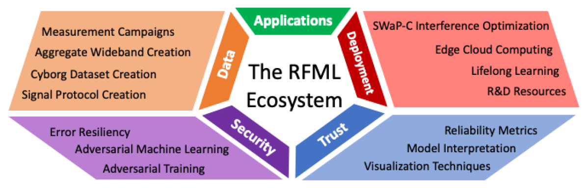
Figure 1: The RFML “Ecosystem” is made up of the major research thrust areas that must be considered holistically in order to utilize RFML systems in real-world applications.

To date, research in applying DL to wireless communications applications, commonly termed RFML, has predominately focused on providing novel solutions that have relied heavily on existing techniques used in other DL modalities applied to the wireless communications application of interest. While this is a logical first step and has shown success, it is expected that the next great leap in RFML capabilities will likely require uniquely tailoring deep learning architectures and techniques to the RF domain using domain specific knowledge, just as CNN were first designed for the unique challenges of the image processing domain.

This paper aims to facilitate this evolution by providing an overview of the key RF domain specific considerations that must be taken into account before deploying RFML solutions in real-world wireless communication applications. More specifically, this paper provides an overview and survey of prior works related to important research areas such as RF dataset formulation (Section III), as well as RFML security (Section IV), trust (Section V), and deployment (Section VI). Through this discussion, particular attention is paid to how all of these areas, the aggregate of which is here termed the RFML “Ecosystem” and illustrated in Figure 1, interact with and affect one another as they are inextricably dependent and therefore must be considered in tandem.

The application of DL to wireless communications applications is a very broad topic area with many different definitions and assumptions. For the discussions and literature review undertaken in this work, RFML is here defined as the usage of DL techniques that aim to reduce the amount of expert defined features and prior knowledge is needed for the intended application. In other words, we predominately consider works in which the input to the RFML system is the raw RF data [2], with some discussion of prior works utilizing or deriving pre-defined expert features.

The current body of literature surveying RFML is copious, yet narrowly focused. More specifically, existing surveys are typically algorithm and/or application focused, and overview, compare, and contrast the learning techniques used and highlight the variety of applications and operating conditions under which RFML is beneficial [3, 4, 5, 6, 7, 8, 9, 10, 11, 12, 13, 14, 15, 16, 17].

A few more unique surveys have also examined RFML dataset generation using GNU Radio [18], the use of big data techniques in wireless networks [19], operational considerations for using cognitive radio in a military setting [20], security and privacy challenges faced in cognitive wireless sensor networks [21], and solutions for combating practical imperfections encountered in cognitive radio system (i.e. noise uncertainty, channel/interference uncertainty, hardware imperfections, signal uncertainty, synchronization issues) [22].

In contrast, the scope of this paper is to holistically bring together these disparate works, highlighting the interdependencies, through the broader RFML “Ecosystem” that underpins them.

II Applications

The RFML ecosystem, as the name implies, is the supporting considerations in the development and deployment of RFML applications. Therefore, before we discuss the different facets of the RFML ecosystem, it is important to provide context through a discussion of the relevant RFML applications found in the literature. An overview of the algorithms described herein, including training data types and algorithm input types, is given in Table I.

ML, and DL in particular, has been applied to a wide variety of areas within wireless communications, including networking applications, power management, and radio control. Given the scope of this paper, as defined above, the applications discussed here tend closer to the physical layer, and can generally be described as spectrum sensing applications.

citation	application	dataset type			input type
		real	synthetic	augmented	raw samples	features
[23]	detection	X			X
[24, 25, 26, 27, 28, 29, 30, 31]		X				X
[32, 33, 34, 35, 36, 37, 38, 39, 40]			X			X
[41]		X	X			X
[42, 43, 44]	classification	X			X
[18, 45, 46, 47, 48, 49, 50, 51, 52, 53, 54, 55, 56, 57]			X		X
[58, 59, 60, 61, 62, 63]		X				X
[64, 65, 66, 67, 68, 69, 70, 71, 72, 73, 74, 75, 76, 77, 78, 79, 80, 81]			X			X
[82]		X			X	X
[83]		X	X			X
[84]		X	X		X	X
[85, 86]			X		X	X
[87]	detection & classification	X			X
[88]			X			X
[89, 90, 91]	parameter estimation		X			X
[92, 13]			X		X
[93, 94, 95, 96]		X				X
[97]	parameter estimation & classification		X		X
[98, 99, 100]	SEI			X		X
[101]		X			X
[102, 103]			X		X
[104]	Anomaly Detection		X			X
[105]			X		X
[106, 107, 108]	DSA		X			X
[109, 110, 111, 112]	Cognitive Radar		X			X
[113]	Cognitive Radio	X			X
[114]		X	X		X
[115, 116]			X		X
[117]			X		X	X

Table I: An overview of the dataset and input types used in popular RFML applications.

II-A Spectrum Sensing

Spectrum sensing is the process of gaining knowledge of a given spectral environment with little, to no, a priori knowledge of the environment. Spectrum sensing is primarily made up of the following DSP tasks: signal detection [118, 24, 32, 33, 34, 23, 35, 87, 25, 36, 88, 26, 37, 27, 41, 28, 38, 39, 40, 29, 30, 31, 89], signal parameter estimation [92, 97, 13, 93, 94, 95, 96], signal classification [58, 18, 87, 42, 64, 65, 83, 66, 67, 68, 59, 45, 69, 70, 71, 60, 43, 61, 72, 73, 97, 74, 46, 62, 63, 75, 76, 77, 47, 84, 48, 49, 50, 78, 85, 79, 80, 88, 86, 51, 52, 44, 53, 54, 55, 119, 56, 81, 57], emitter identification/fingerprinting [98, 101, 102, 99, 100, 103], and anomaly detection [104, 105]. These spectrum sensing tasks are of fundamental importance in both military and commercial applications. For example, in military communications, spectrum sensing is critically important for jamming/anti-jamming, eavesdropping, localization, and demodulation of adversary communications [120]. In commercial communications, spectrum sensing is the primary enabler of DSA in which spectrum users collaboratively utilize spectrum resources without the need for strict, and typically inefficient, spectrum licenses or centralized spectrum managers [106, 107, 108, 109, 110, 111, 112]. Finally, as the quantity of wireless devices continue to grow and rest in the hands of the general public, localization can be a significant tool for a multitude of emergency and safety applications [90, 91], such as search and rescue operations.

II-A1 AMC

One of the earliest, and perhaps the most researched, applications of RFML for spectrum sensing is in the area of modulation classification, likely due to the fact machine learning techniques have historically performed extremely well on classification tasks. Traditional modulation classification techniques typically consist of two signal processing stages: feature extraction and pattern recognition. Traditionally, the feature extraction stage has relied on the use of so-called “expert features” in which a human domain-expert pre-defines a set of signal features that allow for statistical separation of the modulation classes of interest, examples of which can be found in [121]. These expertly defined signal features are extracted from the raw received signal during a potentially time intensive and computationally expensive pre-processing stage. These expert features are then used as input to a pattern recognition algorithm, which might consist of decision trees, support vector machines, feed-forward neural networks, among many others.

RFML based approaches have aimed to replace the human intelligence and domain expertise required to identify and characterize these features using deep neural networks and advanced architectures, such as CNN and RNN, to both blindly and automatically identify separating features and classify signals of interest, with minimal pre-processing and less a priori knowledge [52, 48, 56, 57, 82]. Given the significant research in RFML-based modulation classification, it can be argued that AMC is one of the most mature fields in RFML, and has been deployed in real-world products [122].

II-A2 Signal Detection

Another spectrum sensing area seeing a particular increase in the RFML literature is signal detection [25, 36, 89]. This is one key example in which image processing techniques have been directly applied to solve RFML problems. For example, in [25, 36, 89], the raw IQ samples were converted into spectrum waterfall plots, where the spectrum information in the time-frequency plane is viewed as an image. This has allowed a rich class of image processing techniques to be applied directly to signal detection applications for positive SNR environments.

II-A3 Specific Emitter Identification

SEI, also known as RF Fingerprinting, is an application that has benefited greatly from the advent of RFML [101, 102, 123, 103, 124]. For the purposes of SEI, classification is aimed not towards the transmitted signal, but the transmitter itself, which is possible due to slight (but consistent) differences between emitters, such as IQ imbalances, amplifier non-idealities, and other imperfections caused during the manufacturing process [102], as well as geographical differences such as propagation channels and angle of arrival [125].

These differences not only exist between transmitter brands and models, but amongst transmitters of the same brand and model, which may have been manufactured side-by-side. Due to the difficult nature of defining expert features to distinguish between these subtle differences, the usage of DL within SEI has shown great benefits. More specifically, given the vast number of existing devices, each of which exhibit nearly imperceptible differences, it is near impossible to accurately predict, model, and extract discriminating features. Given these limitations, DL-based solutions, more specifically CNN, which ingest raw RF data, have been used in order to learn the discriminating features for identifying transmitters [101, 102].

II-A4 Parameter Estimation

Parameter estimation is the process of determining relevant discriminating features of a transmitted signal (center frequency, bandwidth, duration, etc) or its propagation channel (time/frequency drifts, shadowing loss, multi-path taps, etc). Often, parameter estimation in RFML is a byproduct of other spectrum sensing tasks. For example, for signal detection applications utilizing spectral waterfall images as input, estimates of the bandwidth, center frequency, and duration are found during the detection process. However, applying RFML directly for parameter estimation has also shown promise, especially in the area of localization.

Localization is incredibly important in both military and commercial communications. Although, traditionally, localization techniques have relied on expert defined features such as received signal strength [126], in recent years a more rich set of RF measurements have been used [126, 94]. In recent work, channel state information is used to reach cm-level accuracy [91] and tackle the difficult problem of indoor 3D (i.e. multi-floor) localization [93]. There has also been progress towards classifying indoor locations using RF samples [95].

II-A5 Anomaly Detection

Finally, an emerging RFML application area is anomalous event detection. In these applications, the intent is for a deep learning approach to learn the baseline environment and detect/classify deviations from this baseline (so-called anomalies). Such applications may also be used to detect adversarial attacks or to identify out-of-distribution examples, as discussed further in Sections IV and V.

An example of this budding area of research can be found in [104], where RF spectrum activities are monitored and analyzed using a deep predictive coding NN to identify anomalous wireless emissions within spectrograms. Similarly, in [105], the authors utilized recurrent neural predictive models to identify anomalies in raw IQ data.

II-B Cognitive Radio

In the literature, the terms RFML and cognitive radio have often been mistakenly used interchangeably. In comparison to the definition of RFML given in Section I, cognitive radio is the use of software-defined radios coupled with state-of-the-art RFML techniques to enable radios to intelligently, and efficiently, utilize its hardware and spectral resources [117]. RFML-based solutions have further enabled the realization of cognitive radio through two keys areas, namely through improved spectrum sensing capabilities (as just discussed) and through direct replacement of fixed signal processing stages with RFML-enabled dynamic stages.

The primary goal of cognitive radio is to adapt to changing channel conditions without needing a human in the loop or time intensive re-configurations. While the usage of RFML-based techniques for supplementing traditional DSP techniques in cognitive radios is still in its infancy, these initial works show promise. One intriguing example of cognitive radio is the use of GAN or AE for end-to-end communications systems design. More specifically, in [13, 113, 115, 116, 114], the authors developed algorithms that allow the neural network model to design the physical layer communications protocol (including modulation scheme, coding scheme, filtering, etc.), using bit or symbol error rate as the performance metric, to overcome the challenge of choosing an appropriate modulation scheme for an unknown, uncharacterized, or changing channel. These approaches have shown promise for both SISO and MIMO radio communications.

III Dataset Creation

In any application of DL, representative and well-labeled datasets are of critical importance for training and/or evaluation. Datasets can generally be categorized into one of three types, namely simulated, captured/collected, and augmented. Simulated datasets refer to synthetically generated data, in which the transmitter, channel, and receiver are all modeled in software/hardware. In contrast, captured datasets are collected from signals that have been transmitted over a wireless channel. Finally, augmented datasets combine simulated and captured data by adding synthetic perturbations to captured data and/or adding synthetic signals to captured channels.

Simulated datasets are the most commonly used in current RFML literature as they are the most straightforward to compile and label using publicly available toolsets such as GNU Radio [127], liquid-dsp [128], and MATLAB [129] among others, and therefore lends itself well to initial development [65, 83, 66, 41, 28, 38, 58, 67, 68, 130, 26, 45, 69, 70, 118, 39, 40, 37, 71, 60, 72, 73, 92, 131, 74, 33, 46, 75, 34, 76, 77, 47, 84, 48, 49, 132, 50, 78, 42, 85, 35, 30, 79, 88, 86, 18, 51, 52, 44, 53, 133, 54, 87, 134, 55, 135, 119, 56, 36, 102, 100]. Unlike in image processing [136], the same equations and processes used to transmit waveforms in real systems can be used directly in simulation, due to their man-made nature [18]. Additionally, for simplistic environments, mathematical models can be used to reasonably describe common degradations such as additive interference, channel effects, and transceiver imperfections. As a result, synthetically generated RFML datasets can be good analogs for captured RFML datasets, if carefully crafted and known models exist.

Captured data is necessary for test and evaluation prior to real-world deployment, but requires significant man-hours and resources to properly collect [41, 28, 59, 26, 60, 43, 61, 24, 29, 62, 98, 63, 84, 137, 101, 23, 80, 88, 44, 27, 138, 25, 36, 93, 94, 95, 96, 99]. This type of data is necessary, because a capture from the real environment will include all of the different degradation types that are of concern in practical RF situations, some of which may be missing from a simulated dataset due to inaccurate modeling; captured data often reduces end user resistance and doubt surrounding the system. As just mentioned, the downside to utilizing capture data are the man-hours and resources required to gather sufficiently diverse captures for producing a training and/or evaluation datasets, and then to label it correctly [46]. This is the fundamental reason that augmented datasets are used, which combine simulated and captured data to increase the quantity of data available for training, or to create more realistic datasets [41, 42, 43, 98, 84, 119].

Finally, while not as optimal as real world data, augmented datasets aim to provide a “best of both worlds” approach by minimizing the limitations of synthetic datasets (i.e. real-world model accuracy) and reducing the amount of captured data needed. At its most basic, augmented datasets shuffle a small subset of real-world data into a larger synthetic dataset. The intent with this approach is to utilize the synthetic data to teach the DL model the features and characteristics of signals that can be well modeled in software (modulation schemes, simple channel models, etc), while the captured data is used to teach the DL model the features and characteristics of signals that cannot be modeled well (i.e. transmitter/receiver imperfections). A more complex augmented dataset might include injecting synthetic waveforms into captured spectrum. Such a dataset would be useful in testing detection and classification performance of the signals in a congested or interference environment with real-world transmitted signals. As another example, synthetic noise could be added to real world captures to decrease the SNR without performing additional signal captures, and increasing the range of test SNR. However, there are a multitude of open research questions in the development and usage of augmented datasets. While many of these questions are application and environment specific, perhaps the most important of these open questions is how to balance the amount of real, synthetic, and augmented data used in training datasets to avoid network bias.

III-A Real World Considerations

No matter the type of dataset being created, there are a number of real-world effects that need to be considered, as they can dramatically impact RFML system performance. When measuring the performance of an RFML device on laboratory-measured or synthetic data versus observed data, the primary difference is often that the trained environment is pristine in comparison to a real environment. This is due to the fact that signals that have propagated in the physical world undergo degradation from multiple overlapping sources not typically encountered in a laboratory. More specifically, both the transmitter and receiver will cause some distortion in the form of non-linearities, additive noise, timing offsets, frequency offsets, phase offsets, sample rate mismatches, and/or amplitude offsets, all potentially time varying, altering the signal from the ideal. Additionally, the physical medium, or channel, through which the signal propagates can change as the transceivers travel around or the environment shifts, allowing delayed imperfect reflections to overlap with the direct path causing time and frequency varying interference with itself.

Depending on the application, the distortion to the waveform caused by the transmitter in particular may be a parameter of interest or may be considered a nuisance parameter requiring an ensemble of emitters to model an average emitter. For example, applications such as SEI depend upon transmitter imperfections to distinguish between emitters. Meanwhile, within AMC transmitter imperfections are considered nuisance parameters, as the goal of AMC is to identify the modulation class, regardless of the emitter. In the case of receiver distortions [46, 126], we find that natural reception variations such as sampling rate differentials, frequency offsets, and varying SNR lead to the requirement for generalized training across each of the parameters [139].

An important note for these hardware variations is that high quality hardware tends to have fewer distortions. For example, military transmitters are often harder to RF fingerprint than low-cost IoT transmitters, and RF signal behaviors learned through a high-quality receiver will translate more easily to another high quality receiver rather than one of lower quality. Moreover, the non-linearities that contribute to these variations are often dependent upon technology and hardware configurations, and lack of synchronization between devices will exacerbate the distortion caused by both the physical medium and the devices. In this case detection and isolation routines are needed to select spectrum of interest, which in turn will introduce measurement errors in time, frequency, and phase offsets between the transceivers. These measurement errors should also be modeled in order create a realistic simulated dataset.

A second area of real-world consideration for RFML system performance is the signal propagation and/or channel effects. The baseline laboratory training environment for virtually all RF systems is an AWGN channel, yet real-world channels have time-varying, often colored spectra, and uncontrolled RF interference sources such as other signals, impulsive noise (i.e. lightning), and non-linear effects associated with bursty packet transmissions. Relative motion between platforms, co-channel/adjacent channel interference, and multi-path should also be considered, yet is often ignored during laboratory training.

Finally, a third consideration, and we believe largely an open problem as we look to scale up the deployment of RFML solutions in real-world scenarios is the use of transfer learning [140, 141], where the behaviors learned and observations collected can be shared between sensors, as well as online or incremental learning, where the behaviors learned are modified over time as a function of a changing environment. For example, automated vehicles could benefit greatly from sharing their observations with the neighboring platforms while operating in a V2V/V2I environment. However, abrupt differences in urban environments and military signal collection/analysis platforms (e.g., ship or UAV) make this challenging. Any future works must consider that the behaviors learned on one platform will be influenced by their RF hardware, which is distinct and possibly vastly different from a second platform. Moreover, the acceptance of online, incremental, and transfer learning poses the significant risks that any learned or transferred behaviors may misrepresent the actual environment (unintentionally or through adversarial interaction), suggesting the need for periodic save points for all relevant parameters.

III-B Developing a Dataset

Taking into account the three types of datasets (simulated, captured, and augmented), and some of the concerns relevant when operating an RFML system outside of a laboratory setting, what follows are general guidelines that should be observed when creating a new RFML dataset. The first step, no matter the type of dataset being created or intended application, is identifying the expected degradations in the deployed environment (i.e. channel types, transmitter imperfections, SNR, etc) and categorizing whether each potential degradation is fundamental to the application. Minimally, each degradation considered fundamental to the application should be described by either

• defining (mathematically) how the degradation is applied, in simulated and augmented datasets, or

• defining the conditions under which the degradation is collected (i.e. hardware used, environment, etc), for captured datasets.

For each identified nuisance degradation, attempts should be made to generalize over observations of the degradation, such as sweeping over the impairment range in simulations or changing the transmission devices or environment in some way while capturing the dataset.

During the dataset creation process, whether through simulation or collection, correctly and completely labelling the data is of the utmost importance. Ideally, though not practically, every parameter should be recorded as metadata associated with the observations in the dataset to increase the number of applications pertinent to the dataset [142]. Qualitative descriptions can also be used to provide as much description as is feasible. Minimally, the parameter of interest to the application (the modulation class in the case of AMC, for example) should be recorded. However, the value of generating and providing datasets with significant diversity, documentation, and open usage rights should not be lost on the community as the gains observed in the image processing domain were realized with the help of crowd sourcing efforts and donations of people’s time [143].

III-C Data Used in Existing Works

A non-exhaustive search for publicly available datasets within RFML turns up datasets released by Geotec [144] for Emitter Localization, DeepSig [145] for AMC, and by Genesys at Northeastern University [146] for RF Fingerprinting. These published datasets were generated for and used in original published works [96, 18, 44, 138], and have created a common point of comparison for different ML approaches within the literature. Though establishing whether these specific datasets can be trusted is outside the scope of the work, knowledge of how the signals in any RF dataset were generated and understanding how to extend/modify said dataset to suit one’s needs is critical in answering whether that dataset can be trusted. Otherwise every signal (and the associated metadata, if applicable) should go through some form of validation by the user, prior to accepting that dataset, but such a validation process is often prohibitive both in computation and time.

Given the limited availability of publicly available RFML datasets, the majority of existing works create their own. For these works and future works, it is critical to describe the parameter space from which the data was generated in the final publication, so that future researchers can reproduce the results. As an example, we consider the signal shown in Figure 2, where two signals have been generated with the same SNR (but with vastly different sampling rates), as defined by

$$\Gamma_{dB}=10\log_{10}\left(\sum_{n\in N}\left|s_{n}\right|^{2}\right)-10\log_{10}\left(\sum_{n\in N}\left|\nu_{n}\right|^{2}\right)$$ (1)

where $s_{n}$ is the $N$ samples of the signal of interest and $\nu_{n}$ is the $N$ samples of AWGN and $\Gamma_{dB}$ is the SNR value in dB. Traditional DSP dictates that the bottom signal can achieve a higher maximum SNR using a matched filter, as is evident in the constellation plots. As most RFML applications describe performance as a function SNR, not including parameters such as sampling rates can greatly impede the ability to reproduce results and can therefore lead to false comparisons in subsequent publications.

Further exacerbating this issue, results could also be described in reference to the energy per bit or $E_{b}/N_{0}$, further creating ambiguity. In this case, the effect of sample rate scaling is already accounted for, but this definition suffers when considering waveforms with no direct definition of $E_{b}/N_{0}$.

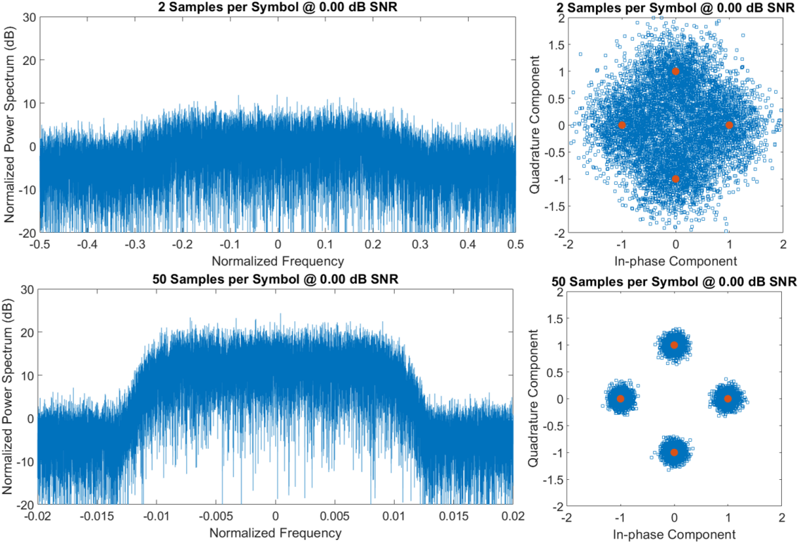
Figure 2: An example of the difficulties of direct comparison when the dataset’s parameters are not explicitly defined. In this case, both signals can claim an SNR value of 0 dB, but the second is significantly oversampled and allows for either preprocessing or learning a filter-like behavior raising the apparent SNR observed during processing.

IV Security

While AI/ML has been adopted in some format in nearly all industries in recent years, it’s limitations in adversarial settings have been well documented in modalities such as CV [147], audio recognition [148, 149, 150], and NLP [151]. While the attacks demonstrated in other modalities serve as a prescient warning for applications of RFML and many parallels can be drawn, recent work has shown there are unique considerations for AI security in the context of RF due to the nature of wireless propagation, pre-processing steps before RF signals of interest are input to DNN, and the fact that wireless communications are generally quite sensitive to perturbations in the transmission. Therefore, while this section provides a brief overview of AI security in general, the focus is on the unique considerations in RFML for which a Threat Model is provided in Figure 3 which quickly categorizes the related work in the area.

Figure 3: Threat Model for RFML adopted from [160, 156] and including related work.

IV-A Adversarial Machine Learning

When discussing AI security, the conversation primarily revolves around Adversarial ML which concerns the development of algorithms to attack data driven models and to defend against such attacks. Discussions of Adversarial ML [161, 162] date back at least 15 years [163, 164, 165] and have broadened to include exploratory attacks that seek to learn information about (or replicate) the classifier [166] or training data [167] through limited probes on the model to observe it’s input/output relationship. However, the most recent explosion in concern for the vulnerabilities of DNN specifically is largely credited to the FGSM attack [168] which showed that CV models are vulnerable to small, human imperceptible, perturbations to their input images that cause a misclassification – and these perturbations are relatively computationally cheap to create, requiring only a single back-propagation instead of a costly optimization loop. This manipulation of the model’s inputs to achieve a goal such as misclassification (not classified as the true class of the input) or targeted misclassification (forcing the model to classify the input as a specific and different class) is termed an evasion attack and is the most widely studied sub-field of Adversarial ML, including in RFML.

It should also be noted that while this section focuses primarily on attacks on signal classification, the adversarial attacks can be more broadly applied to other RFML tasks. Generally speaking, an evasion attack influences the input of a DNN to change its output. Therefore, any application of DNN for spectrum sensing or cognitive radio discussed in Section II is susceptible to attack.

IV-A1 Evasion

Evasion attacks are most prevalent in the study of classification tasks where a key constraint in these attacks is to ensure they remain imperceptible to the intended receiver, which is uniquely defined in the context of wireless. Evasion attacks can further be categorized as untargeted or targeted digital attacks, as will be discussed further below.

Untargeted Digital Attacks

Untargeted digital attacks can be defined as evasion attacks in which the goal is solely misclassification. RFML models have been shown to be just as vulnerable to these untargeted adversarial attacks as their DNN counterparts in CV. Specifically, both [133] and [156] showed that the FGSM attack is sufficient to completely evade AMC by a DNN with a perturbation that is 10 dB below the actual signal. While FGSM is a computationally cheap method for creating adversarial examples, the large body of literature in adversarial ML for CV has yielded algorithms that can evade classifiers with even smaller perturbations. In [159], a more sophisticated adversarial methodology [169] was used to carry out an attack on AMC; not only was this attack successful for a DNN, but, when the adversarial examples were input to classifiers not based on DNN (e.g. SVM, Decision Trees, Random Forests, etc.) the models had similar decreases in accuracy. Therefore, although adversarial ML methodologies use DNN to craft adversarial examples due to the need for back propagation, they are transferable across various classification methodologies. Thus, the perturbations cannot simply be noise specific to a DNN model, they must be changing something inherent to the signal properties that are used by many methodologies for classification.

Targeted Digital Attacks

As previously mentioned, the goal of targeted digital attacks is to force a model to make a specific misclassification. By more closely examining how AMC DNN break down under evasion attacks, other work has also shown that Adversarial ML takes advantage of something inherent to the properties of man-made signals. More specifically, modulation formats for wireless communications are man made; thus, they can be intuitively grouped into a hierarchical structure. For instance, analog modulations, such as the Amplitude Modulation and Frequency Modulation used in older vehicle radios, are distinctly separate from digital modulations used to carry discrete symbols representing the bits of a data transmission. Within digital modulations, the formats can be hierarchically grouped into whether they represent symbols in the frequency domain (FSK), in the signal’s phase (PSK), or in both the signal’s phase and amplitude (QAM). One would expect that a DNN would learn this intuitive grouping as well and therefore it would more easily confuse an analog modulation with another analog modulation than it would mislabel an analog modulation as a digital transmission. In fact, [153] used the Momentum Iterative FGSM [170] attack to show that this is precisely the case. The authors showed that higher power adversarial perturbations are required to move between source/target pairs belonging to different coarse-grained categories than to target a class belonging to the same category as the source signal.

Rubbish Class Examples/Fooling Images

Other research has considered the ability to create examples that are classified as some target class but have no semantic meaning, commonly referred to as Rubbish Class Examples [168], Fooling Images [171], or, in the context of wireless communications, Spoofing Attacks [172]. While a Spoofing Attack may provide benefits over a simpler Relay Attack by considering channel and receiver effects in the adversarial transmission, no communication can occur using such an attack. Therefore, the benefits of such an attack would be limited and the more prevalent threat is considering how signals can be manipulated without losing their underlying semantic meaning.

Defining Perceptible Perturbations in Wireless

The main constraint in adversarial machine learning is generally provided, particularly in CV, as a constraint on the perturbation power, a proxy for the notion of perceptibility of the perturbation (e.g. does this perturbation affect a human observer’s judgement of the image, interpretation of the audio signal content, or reading of a sentence). This notion is more easily defined in RFML as the BER at a receiver. More specifically, because the receiver is blind to the perturbation being applied, BER defines the perceptibility of the adversarial attack [156] (i.e. the more obvious the perturbation, the higher the BER). Therefore, recent work has created differentiable versions of receive chains, that allow for the BER to be directly incorporated into the loss function of an adversarial attack [155, 157]. Thus, even though attacks transferred from CV may have lower utility in wireless communications due to their large impact on the wireless transmission, the attackers will continue to evolve specifically in the context of RFML, leading to more sophisticated threats. As such, defenses must be investigated that mitigate future threats to RFML systems being deployed in high risk adversarial environments.

IV-A2 Defense

Defending against adversarial attacks can be roughly split into two categories, discussed further in the following subsections:

1. detecting an attack is occurring in order to take counter-measures, or

2. becoming robust to attacks by increasing the power of the perturbation required to cause a misclassification.

While this section only focuses on the work that has been done specifically for RFML in the context of adversarial evasion attacks, more general surveys on adversarial attacks and defenses are provided in [161, 173]. Further, a more general discussion of detecting whether an example is in distribution is left to Section V.

Detecting Attacks

Detecting an attack can be thought of as a supplemental binary classification that determines is this example in or out of distribution? Two metrics are proposed in [174] for detecting adversarial attacks on wireless communications. The first uses the distribution of the PAPR of the underlying signal along with the model’s classification. Since the PAPR can be used as a signature for a given modulation, the work in [174] tests whether the DNN classification and PAPR signature are in agreement on the classification; if not, then the example is assumed to be an adversarial example. This test is specific to the RFML task, AMC, but agnostic of the model used. The second test uses the distribution of the output probabilities of the DNN to determine whether an example is in or out of distribution and is therefore agnostic of the task it is applied to. However, performing statistical tests during inference can increase system complexity on an already SWaP constrained RFML system (discussed further in Section VI) leading to increased classification latency and thus decreased bandwidths that can be sensed in real time. Additionally, this additional check can be incorporated into the attack, once the attacker has become aware, and likely bypassed just as the original classification was [175]. Therefore, pushing the defense methodology into the training stage of the DNN, where the computational complexity can be handled off target and without a time constraint, is often beneficial.

Becoming Robust to Attacks

The most widely used methodology for gaining robustness is adversarial training [168, 176, 177, 178, 179]. Adversarial training is simply the introduction of correctly labeled adversarial examples during training time by a known adversarial attack (such as FGSM). Another method that alters the training strategy of DNN to confer robustness is to reduce the degrees of freedom of an attacker by lowering the input dimensionality. The work in [180] adopted both strategies for training and observed that it increased the model’s robustness to FGSM attacks. The results of [180] also showed that lowering the input dimensionality alone was sufficient to increase robustness to an FGSM attack; however, that adversarial training decreased the number of training epochs needed to reach near perfect accuracy on legitimate examples. This highlights that adversarial training is not only good for conferring robustness, but can also be used a data augmentation technique for RFML (Section III). However, no work (yet) has shown that an adversarially trained classifier would be robust to all attack methodologies [170].

Moving Towards Mathematically Rigorous Definitions of Robustness

Given that many proposed defenses have been quickly proven to be inadequate, it is important to be overly cautious when evaluating a new methodology [181]. In addition to evaluating defenses against a huge, and growing, list of adversarial attacks (using an open source library such as Cleverhans can help alleviate the development burden [182]) research has begun looking into provable robustness. One such work is [183] that uses the Lipschitz function of DNN to provide a lower bound on the adversarial distance needed to cause a misclassification. More generally, this concept is about whether the model can be trusted on real inputs, where the inputs are distorted by some perturbation, regardless of whether the perturbations are man-made or naturally occurring. Therefore, this discussion is deferred to Section V.

IV-B Mitigation Through Standard Security Practices

Defending a RFML system from attack does not have to only revolve around adversarial ML based defenses. By using standard cybersecurity best practices, an adversary can be forced to move down the Threat Model presented in Figure 3 by having their knowledge of and access to the RFML system limited. Therefore, the attacks become much more difficult to successfully execute.

More specifically, most adversarial attacks and defenses are proposed and evaluated in a fully digital world (a digital attack in Figure 3); however, such attacks and defenses can transfer to the physical environment as well [184]. In the context of RFML, this physical environment means that the perturbation is radiated from an external transmitter. Therefore, the transmission is impacted by channel effects, hardware impairments at both the transmitter and receiver, and DSP pre-preprocessing techniques before reaching the DNN for classification (a physical attack in Figure 3). All of these can serve as an impediment for an attacker, forcing them to raise their adversarial perturbation power in order to overcome the effects [156, 157, 185, 159].

Additionally, so-called white-box attacks, which assume full knowledge of the target DNN, are generally known to be more effective than black-box attacks which assume close to zero knowledge about the target, regardless of modality. This is not meant to say that adversarial examples do not transfer between models, only that when transferring adversarial examples between models, a small penalty on the adversary’s success is incurred. However, limiting the amount of information an adversary can build up about the DNN is a critical first step in defending against attack.

IV-C Discussion and Future Work

The broader community’s understanding of adversarial examples in terms of how to create and defend against them, when to inject them into a DNN (training/inference), and why they exist, is still rapidly evolving. Much of this discussion can be applied generally across all data modalities; however, RFML provides unique considerations that must also be studied separately:

1. the physical channels between adversary and receiver are significantly different,

2. the perceptability of the perturbation is machine defined, not human defined, and

3. the actions taken based on the generated knowledge are application specific.

Due to i. and ii., adversarial attacks from other modalities are of limited concern to deployed RFML systems as the wireless channel forces the adversary to increase the perturbation power to a level that significantly interferes with the primary objective of the transmission: to communicate. Ongoing work has shown that more sophisticated attacks will emerge to overcome these limitations by incorporating more expert knowledge (i.e. channel type [186], channel coding scheme[187], device type[188]) into the adversarial process. Another key research direction going forward is determining what information is emitted from a RFML device, such as acknowledgement messages or transmission decisions [188, 189], that can aid in online learning for increased attack effectiveness. Finally, a major benefit of a RFML controlled radio over a traditionally deterministic policy based approach is the ability of the radio to continually learn and adapt to its specific environment. Thus, the recent work in determining how the training data of RFML systems can be manipulated to cause a degradation in model performance [152, 190] will motivate the study of data cleaning methodologies for wireless.

V Trust and Assurance

For all RFML applications (Section II), there is a desire to translate laboratory performance into a user-defined mission assurance. This is critical to not only assuring that the machine learned behaviors, which are difficult to reverse engineer, behave as expected when put to practice, but more importantly, understanding how the system will respond to unanticipated stimuli and/or recognizing that an input is outside the training set of its learned responses. Taking this need to an extreme, a significant amount of end-user confidence is required to give RFML systems the authority to permit autonomous weapons release [191].

In most current RFML techniques evaluated, learned behaviors are a function of correlation rather than causation. That is, algorithms are data-driven, and thereby assume that the training, validation, and test datasets used to develop said algorithm are drawn from the same distribution which will be seen once deployed. A primary concern for early adopters of RFML is how the algorithm will behave when this assumption is invalid, either due to the real-world considerations not present in the training data or adversarial attack as discussed in Sections III, IV, and VI.

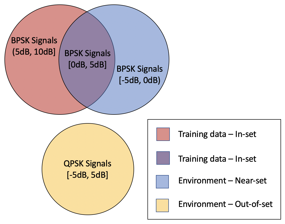
Figure 4: An example of in-set, near-set, and out-of-set data types for an RFML algorithm trained on BPSK signals with SNRs between 0dB and 10dB.

In other words, we can categorize inputs in one of three ways, illustrated in Figure 4:

• in-set - Those that match the distribution of the training data. Using modulation classification as an example, an in-set input is a known modulation scheme under the same channel effects, SNR, transmitter/receiver imperfections, etc. that were seen during training.

• near-set - Those close to the distribution of the training dataset, but not included. In our modulation classification example, near-set inputs might be a trained modulation scheme, but different channel effects or SNR.

• out-of-set - Those completely outside of the distribution of the training data. Completing our example, an out-of-set example would be an untrained modulation scheme.

A data-driven RFML system will behave as expected on in-set inputs, but is unpredictable on near-set input values, and necessarily incorrect in processing all out-of-set input values. This points to a critical need for approaches to both rigorously assure “the safety and functional correctness” of RFML systems throughout deployment [192] and explain or understand the behavior of RFML systems [193].

These concerns are not unique to RFML [194], but have yet to be adequately addressed in RFML literature. Therefore, this section will focus on the very young body of work in testing, verification, and interpretation of general ML systems which could be explored for use in the RF domain, and will discuss the pros and cons of the various approaches. These works can broadly be categorized into three research areas,

• verification methods which provide mathematical proof that a desired property holds for a trained model,

• testing methods which aim to exhaustively evaluate a trained model to identify flaws, and

• interpretation/explanation techniques which include methods to describe and/or quantify a trained model’s learned behaviors in a human-understandable format, such as decision/model explanations or uncertainty/reliability metrics.

V-A Verification

Beginning with the most rigorous approaches, current methods for verifying ML algorithms apply formal methods such as constraint solving [195, 196, 197], global optimization [198], search-based methods [199], and over approximation [200] to provide provable guarantees about their behavior when provided with in-set, near-set, out-of-set, and even adversarial examples. While verification methods provide deterministic or statistical guarantees of the robustness of previously trained models, they are also typically NP hard or extremely computationally expensive and time intensive. As a result, none have been able to successfully scale to the state-of-the-art deep NN used today.

Towards scalable ML verification methods, a promising path forward is that of approximate or iterative/anytime methods which provide provable upper/lower bounds or monotonically converging bounds [198, 197, 200, 199]. However, future work is needed to improve these methods, in order to yield tighter and more useful bounds on the robustness of trained models.

V-B Testing

Traditionally, ML researchers and engineers rely on a held-out test set, which remains unseen throughout the training and model selection process, to provide an estimate of a trained model’s performance [201]. This computationally efficient method provides a good estimate of how the model will perform on in-set data, but fails to identify how the model will perform on near-set or out-of-set data.

In an effort to strike a balance between computational efficiency and rigorousness, there is a growing body of work adapting and applying software testing and debugging techniques to more thoroughly test ML algorithms. These approaches generate test cases using methods such as concolic testing [202, 203], mutation testing [204], differential analysis [205], or even adversarial methods [206], which is typically guided by a user-selected coverage metric. Some of the most popular coverage metrics used have included neuron or layer coverage [207, 208] and modified condition/decision coverage [202]. The aim is to generate a set of test cases/inputs which provide sufficient coverage of the trained model, dictated by a user-selected threshold.

Though test case generation may provide more assurance than traditional ML testing practices and are typically more computationally efficient than verification methods, there are a number of drawbacks which should be addressed. First and foremost, like traditional software testing methods, ML testing methods can only identify a lack of robustness, and cannot ensure robustness. In the same vein, the effectiveness of the testing method is highly dependent upon the coverage metrics and thresholds used, both of which are chosen by the user. With some coverage metrics and thresholds, testing methods may be just as computationally expensive and time consuming in comparison to approximate verification methods. Ultimately, while there is certainly value in more effective testing techniques, future work will likely need to focus on RFML verification over RFML testing, in order to effectively mitigate against adversarial attack and provide assured performance [209].

V-C Interpretation/Explanation

Switching gears, the aim of interpretation/explanation methods is to address the challenge of HMI by “enabl[ing] users to understand how the data is processed and supports awareness of possible bias and systems malfunctions” [210]. In other words, HMI becomes more feasible if the model/decision is better understood by the end user. Approaches to interpret or explain black-box ML models such as deep NNs and/or their decisions can broadly be categorized into two groups.

The first group of approaches provide intrinsic interpretability by using inherently more interpretable models either from the offset or extracted from a black box model [211]. Examples of such models include decision trees [212, 213], attention mechanisms [214], clustering algorithms, or linear/Bayesian classifiers [215]. While these methods are typically the most straightforward and provide the most useful model/decision explanations, inherently interpretable models are typically less expressive than black-box models such as deep NN, and therefore do not provide the same level of performance.

The second group of approaches provide post-hoc interpretability by extracting decision/model explanations from black-box models or through model exploration [211, 210]. Post-hoc interpretability methods can be further broken down into local interpretability methods and global interpretability methods. Local interpretability methods aim to provide an explanation for why and/or how a black box model made the decision it made for a given example input. These instance-level explanations can be aggregated over a group of example inputs to draw larger conclusions about a model’s knowledge. Meanwhile global interpretability methods focus on increasing the transparency of black-box models by “inspecting the structures and parameters” in an effort to understand the scope of the model’s knowledge more directly [211].

Local interpretability methods typically utilize some form of visualization to describe the network’s response to the input such as heatmaps, which indicate which portions of the example input contributed most to the network’s decision [216, 217]. Popular and successful local interpretability methods in the image processing domain include backpropagation techniques such as layerwise relevance propagation, Taylor decomposition, and GradCAM [216, 218, 219], saliency mapping [217], and deconvolutional networks [220]. However, transitioning these methods to the RF domain has proven challenging, as raw RF data is more difficult to visualize, especially in the intermediate layers of a deep NN. Therefore, a more promising local interpretability method for use in the RF domain is the use of uncertainty metrics to accurately quantify a model’s confidence in any given decision, and could be used to identify unpredictability due to adversarial attack or operating environments [221, 222].

Global interpretability methods focus less on visualization techniques due to the large number of parameters in deep NN models, but have been explored through approaches such as activation maximization and partial dependence [217, 223, 224, 225]. More common is the use of metrics such as feature importance [226, 227], sensitivity [228, 229], and mutual information [230].

The primary challenge shared amongst both local and global interpretability methods is that there are no universal definitions for terms such as trust, interpretability, assurance, and explanation in the deep learning literature. Furthermore, the concept of interpretability is highly dependent on the end user and their technical background [231]. For example, some argue that while global interpretability methods are useful to the deep learning expert who understands the inner-workings of a black-box model, local interpretability methods are more tangible, intuitive, and provide more benefit to the end user. Furthermore, trust, interpretability, assurance, and explanation are largely gauged qualitatively rather than quantitatively, and therefore are hard to compare and evaluate across approaches [210].

Additional challenges to ML interpretations include, but are not limited to [194]:

• How to accurately characterize and/or classify out-of-set examples. This is one area where uncertainty metrics would likely be more useful than visualization based explanation methods

• Producing consistent explanations for similar inputs

• Producing explanations without significant computational overhead

• Deep NN produce an overwhelming amount of highly complex and interdependent data that is difficult to visualize, describe, and/or explain in a helpful manner. The abstract nature of RF data only exacerbates this challenge.

V-D Discussion

Trust/assurance in RFML systems will likely require some form of both verification method in conjunction with interpretation/explanation methods [232], in order to provide designer, administrator, operator, and end-user confidence in a model’s decision-making capabilities both before and during deployment. As discussed above, interpretation/explanation methods provide the user with an intuitive and/or quantifiable level of confidence in a model’s decision, improving their understanding of and trust in the system. While this understanding and trust is critical to HMI, assured RFML suitable for use in safety-critical systems, such as self-driving cars and military systems, will require the rigorous guarantees that verification provides.

VI Deployment

Early adoption of RFML systems has already taken place in a variety of military systems [233, 2, 122, 234], though a broader interest will exist for the rollout of commercial cellular [235, 236, 237], the IoT [238, 103, 239, 240], and even satellite communications [241, 242, 243]. Given the breadth of applications identified for RF machine learning techniques given in Section II, there is a fundamental desire to transition the developed techniques to real systems. This section evaluates the practical constraints of size, weight, power, cost, and performance bounds to facilitate deployment.

VI-A Size, Weight, Power, and Cost (SWaP-C)

Beginning with size and weight, it is notable that many DL techniques employ significant computing infrastructures during their training phases, the scope of which makes them infeasible for training in the field; however, we are most concerned with the DL algorithm’s computational requirements when attempting to process incoming, unknown, data inputs once deployed post training [244]. One advantage of RFML techniques, as compared to most CV techniques, is that the sizes of the associate NN and processing are drastically smaller – in many cases 2-3 orders of magnitude smaller in terms of number of parameters and thus memory utilization. Further, some RFML implementations incorporate pre-calculated traditional signal processing techniques such as Fourier and wavelet transforms, cyclostationary feature estimators, and other expert features to serve as a more efficient feature that may be merged with machine learned behaviors [245, 241, 246]. Other research has focused on reduced precision implementations of machine learning structures as a method to gain computational efficiency [247, 248, 249]. However, the use of online learning techniques in RF scenarios requires real-time computational resources that are currently difficult to reduce to a mobile system [250, 251], in addition to the challenges discussed in Section III.

Given the highly effective miniaturization of digital electronics, a deployed system’s weight is primarily driven by its power consumption and the associated batteries or heatsinks [252]. As such, real-time evaluation of signal detection [253], signal characterization [122], and specific emitter identification [103] have each been evaluated, with the latter two being implementable to a tactical/mobile use case, either through the assumption of vehicle power or a tightly regulated and small duty cycle. Driving system criteria for this power usage include the instantaneous bandwidth of the spectrum analyzed, the density of signals within the environment (affecting the number of calls to an RFML function), implementation in software versus hardware, and the environment where the device is used. The use of wake-up circuits for periodic/event-triggered execution of a RFML function can be used to drastically reduce average power draw [103]. Additionally, the use of energy harvesting techniques, and RFML processing within those energy production envelopes, are of particular interest for battery-powered IoT and solar-powered satellites.

Beyond SWaP, cost is typically the next important deployment consideration. To date, the primary cost of RFML systems appears to be underlying datasets used for training, followed by the training process and hardware, and finally by the fieldsets to be deployed. As discussed previously in Section III, the quality of the data drives overall functionality, and often requires human-intensive labeling and/or pre-processing [2]. Training costs are primarily driven by the purchase and use of parallelized processors such as Graphics Processing Units, Tensor Processing Units, or other special purpose hardware. Both the data collection and training processes can be amortized over the number of fieldsets – in current military deployments, the number of deployed units is typically small, making the relative cost per mobile fieldset high. By contrast, deployment for a widely used 5G/6G cellular application will be make the training costs, if broadly applicable, nearly negligible.

VI-B Application Dependencies

As described in Sections II and III, the scale and scope of different applications can lead to vastly different hardware and SWaP requirements – at one end of the spectrum a Raspberry Pi 0 for performing event-triggered packet-based SEI for IoT networks [103] and on the other end a real-time 5 GHz instantaneous continuous spectrum monitoring system [2]. One specific application example, driven by environmental effects, is the potential deployment of ML algorithms aboard small spacecraft, which are impacted by radiation-induced single event upsets [254, 255] – without the addition of radiation shielding and/or extensive mitigation strategies, the performance of the ML structures fail to achieve the necessary performance [256, 257, 258, 259, 260, 261] to be practically useful. Broader dependencies include harnessing the more rapid decision making of RFML - in many applications discussed in Section II, the envisioned use case for RFML is primarily as a decision aid. Additional work will be required to make the raw observables fully actionable in live systems.

VI-C Open Questions for Deployment

In addition to those described previously in this section, we see the need for future research that addresses the following capabilities before RFML algorithms can supplant existing techniques.

• Online, incremental, and transfer learning techniques: current training processes generally assume up front training with a defined set of signal classes or RF environmental conditions. Work is needed to add new signals or emitters without repeating the training process, as discussed previously in Section III.

• New processing capabilities: expanding upon work for reduced-precision implementations of neural nets, research is needed to evaluate more computationally efficient designs, such as pruning, bit-slice processor architectures for offline/intermittent calculation, potential insertion of RFML math co-processors during execution stages, etc.

• Online learning: given the real-time nature of spectral observations, there is a need to improve the efficiency and timeline of online learning that absorbs new information into the trained behaviors.

• Distributed RFML: most current work is focused on individual nodes, yet many RF systems offer the potential of multiple apertures whose spectrum observations can be integrated to gain a larger system picture, as briefly mentioned in the context of transfer learning in Section III. Example applications for expansion include multi-node geo-location and transfer learning using compressed samples or intermediate outputs of the RFML processing.

• Human interaction with RFML: beyond individual decisions for signal detection or classification, additional work is needed in helping the end user understand the limits of the learned behaviors, how to shape and/or optimize use the system, and how to visualize and/or verify whether the machine should be trusted, a topic further explored in Section V.

• Confidence: also discussed further in Section V as well as in Section IV, additional work is required to identify in real-time if prior training is truly representative of decisions requested as well as the quality of the resulting decision (i.e. consistency with laboratory-calculated performance) in order to provide assured performance, as well as to begin ruggedizing the decision chain against spoofing and other adversarial techniques

VII Conclusion

As shown in Section II, RFML is a rapidly growing area of research, due to its demonstrated success in improving and automating spectrum sensing applications and supporting next-generation cognitive/intelligent radio applications. However, these works have primarily focused on conforming existing image or natural language processing solutions to an RF application, each making their own assumptions about dataset availability, use cases, etc, and often ignoring key considerations, common to all RFML solutions, that must be addressed in order to make deployable RFML technologies realizable.

In this work, these common considerations, termed the “RFML Ecosystem” were defined as the application itself (Section II), dataset creation (Section III), security (Section IV), trust and assurance (Section V), and deployment (Section VI). For each element of the ecosystem, along with an overview of the topic, the primary research areas were identified with examples of existing works. Additionally, discussion of dependencies between the elements of the RFML ecosystem provide a comprehensive and integrated summary of the domain-specific challenges to applying DL to RF. In whole, this work aims to be a holistic guide for RFML developers looking to develop realizable and deployable solutions for real-world applications and to promote the advancement of ML architectures and algorithms purpose-built for the RF domain.

References

- [1] M. E. Morocho-Cayamcela, H. Lee, and W. Lim, “Machine learning for 5G/B5G mobile and wireless communications: Potential, limitations, and future directions,” IEEE Access, vol. 7, pp. 137 184–137 206, 2019.
- [2] T. Rondeau, “Radio frequency machine learning systems (RFMLS).” [Online]. Available: https://www.darpa.mil/program/radio-frequency-machine-learning-systems
- [3] M. Alshawaqfeh, X. Wang, A. R. Ekti, M. Z. Shakir, K. Qaraqe, and E. Serpedin, “A survey of machine learning algorithms and their applications in cognitive radio,” in International Conference on Cognitive Radio Oriented Wireless Networks. Springer, 2015, pp. 790–801.
- [4] H. K. Jhajj, R. Garg, and N. Saluja, “Aspects of machine learning in cognitive radio networks,” in Progress in Advanced Computing and Intelligent Engineering, K. Saeed, N. Chaki, B. Pati, S. Bakshi, and D. P. Mohapatra, Eds. Singapore: Springer Singapore, 2018, pp. 553–559.
- [5] M. A. Alsheikh, S. Lin, D. Niyato, and H. Tan, “Machine learning in wireless sensor networks: Algorithms, strategies, and applications,” IEEE Communications Surveys Tutorials, vol. 16, no. 4, pp. 1996–2018, Fourthquarter 2014.
- [6] R. Boutaba, M. A. Salahuddin, N. Limam, S. Ayoubi, N. Shahriar, F. Estrada-Solano, and O. M. Caicedo, “A comprehensive survey on machine learning for networking: evolution, applications and research opportunities,” Journal of Internet Services and Applications, vol. 9, no. 1, p. 16, 2018.
- [7] Y. Sun, M. Peng, Y. Zhou, Y. Huang, and S. Mao, “Application of machine learning in wireless networks: Key techniques and open issues,” IEEE Communications Surveys Tutorials, vol. 21, no. 4, pp. 3072–3108, Fourthquarter 2019.
- [8] Ma Di and Er Meng Joo, “A survey of machine learning in wireless sensor networks from networking and application perspectives,” in 2007 6th International Conference on Information, Communications Signal Processing, Dec 2007, pp. 1–5.
- [9] Q. Mao, F. Hu, and Q. Hao, “Deep learning for intelligent wireless networks: A comprehensive survey,” IEEE Communications Surveys Tutorials, vol. 20, no. 4, pp. 2595–2621, Fourthquarter 2018.
- [10] C. Clancy, J. Hecker, E. Stuntebeck, and T. O’Shea, “Applications of machine learning to cognitive radio networks,” IEEE Wireless Communications, vol. 14, no. 4, pp. 47–52, August 2007.
- [11] G. P. Joshi, S. Y. Nam, and S. W. Kim, “Cognitive radio wireless sensor networks: applications, challenges and research trends,” Sensors, vol. 13, no. 9, pp. 11 196–11 228, 2013.
- [12] T. Erpek, T. J. O’Shea, Y. E. Sagduyu, Y. Shi, and T. C. Clancy, Deep Learning for Wireless Communications. Cham: Springer International Publishing, 2020, pp. 223–266. [Online]. Available: https://doi.org/10.1007/978-3-030-31764-5_9
- [13] T. O’Shea and J. Hoydis, “An introduction to deep learning for the physical layer,” IEEE Transactions on Cognitive Communications and Networking, vol. 3, no. 4, pp. 563–575, 2017.
- [14] M. Chen, U. Challita, W. Saad, C. Yin, and M. Debbah, “Artificial neural networks-based machine learning for wireless networks: A tutorial,” IEEE Communications Surveys Tutorials, vol. 21, no. 4, pp. 3039–3071, Fourthquarter 2019.
- [15] M. Bkassiny, Y. Li, and S. K. Jayaweera, “A survey on machine-learning techniques in cognitive radios,” IEEE Communications Surveys Tutorials, vol. 15, no. 3, pp. 1136–1159, Third 2013.
- [16] C. Jiang, H. Zhang, Y. Ren, Z. Han, K. Chen, and L. Hanzo, “Machine learning paradigms for next-generation wireless networks,” IEEE Wireless Communications, vol. 24, no. 2, pp. 98–105, April 2017.
- [17] O. Simeone, “A very brief introduction to machine learning with applications to communication systems,” IEEE Transactions on Cognitive Communications and Networking, vol. 4, no. 4, pp. 648–664, Dec 2018.
- [18] T. J. O’shea and N. West, “Radio machine learning dataset generation with GNU Radio,” in Proceedings of the GNU Radio Conference, vol. 1, no. 1, 2016.
- [19] M. G. Kibria, K. Nguyen, G. P. Villardi, O. Zhao, K. Ishizu, and F. Kojima, “Big data analytics, machine learning, and artificial intelligence in next-generation wireless networks,” IEEE Access, vol. 6, pp. 32 328–32 338, 2018.
- [20] T. Tuukkanen and J. Anteroinen, “Framework to develop military operational understanding of cognitive radio,” in 2015 International Conference on Military Communications and Information Systems (ICMCIS), May 2015, pp. 1–9.
- [21] J. Sen, “Security and privacy challenges in cognitive wireless sensor networks,” in Cognitive Radio Technology Applications for Wireless and Mobile Ad hoc Networks. IGI Global, 2013, pp. 194–232.
- [22] S. K. Sharma, T. E. Bogale, S. Chatzinotas, B. Ottersten, L. B. Le, and X. Wang, “Cognitive radio techniques under practical imperfections: A survey,” IEEE Communications Surveys Tutorials, vol. 17, no. 4, pp. 1858–1884, Fourthquarter 2015.
- [23] S. Mohammed, R. El Abdessamad, R. Saadane, and K. A. Hatim, “Performance evaluation of spectrum sensing implementation using artificial neural networks and energy detection method,” in 2018 International Conference on Electronics, Control, Optimization and Computer Science (ICECOCS), Dec 2018, pp. 1–6.
- [24] M. R. Vyas, D. K. Patel, and M. Lopez-Benitez, “Artificial neural network based hybrid spectrum sensing scheme for cognitive radio,” in 2017 IEEE 28th Annual International Symposium on Personal, Indoor, and Mobile Radio Communications (PIMRC), Oct 2017, pp. 1–7.
- [25] T. J. O’Shea, T. Roy, and T. Erpek, “Spectral detection and localization of radio events with learned convolutional neural features,” in 2017 25th European Signal Processing Conference (EUSIPCO), Aug 2017, pp. 331–335.
- [26] D. Pu, Y. Shi, A. V. Ilyashenko, and A. M. Wyglinski, “Detecting primary user emulation attack in cognitive radio networks,” in 2011 IEEE Global Telecommunications Conference - GLOBECOM 2011, Dec 2011, pp. 1–5.
- [27] S. Yi, H. Wang, W. Xue, X. Fan, L. Wang, J. Tian, and R. Matsukura, “Interference source identification for IEEE 802.15.4 wireless sensor networks using deep learning,” in 2018 IEEE 29th Annual International Symposium on Personal, Indoor and Mobile Radio Communications (PIMRC), Sep. 2018, pp. 1–7.
- [28] F. Ge, Q. Chen, Y. Wang, C. W. Bostian, T. W. Rondeau, and B. Le, “Cognitive radio: From spectrum sharing to adaptive learning and reconfiguration,” in 2008 IEEE Aerospace Conference, March 2008, pp. 1–10.
- [29] S. S. Fernandes, M. R. Makiuchi, M. V. Lamar, and J. L. Bordim, “An adaptive recurrent neural network model dedicated to opportunistic communication in wireless networks,” in 2018 International Joint Conference on Neural Networks (IJCNN), July 2018, pp. 01–08.
- [30] A. Subekti, H. F. Pardede, R. Sustika, and Suyoto, “Spectrum sensing for cognitive radio using deep autoencoder neural network and SVM,” in 2018 International Conference on Radar, Antenna, Microwave, Electronics, and Telecommunications (ICRAMET), Nov 2018, pp. 81–85.
- [31] F. Wunsch, F. Paisana, S. Rajendran, A. Selim, P. Alvarez, S. Müller, S. Koslowski, B. Van den Bergh, and S. Pollin, “DySPAN spectrum challenge: Situational awareness and opportunistic spectrum access benchmarked,” IEEE Transactions on Cognitive Communications and Networking, vol. 3, no. 3, pp. 550–562, Sep. 2017.
- [32] D. Han, G. C. Sobabe, C. Zhang, X. Bai, Z. Wang, S. Liu, and B. Guo, “Spectrum sensing for cognitive radio based on convolution neural network,” in 2017 10th International Congress on Image and Signal Processing, BioMedical Engineering and Informatics (CISP-BMEI), Oct 2017, pp. 1–6.
- [33] R. G. Yelalwar and Y. Ravinder, “Artificial neural network based approach for spectrum sensing in cognitive radio,” in 2018 International Conference on Wireless Communications, Signal Processing and Networking (WiSPNET), March 2018, pp. 1–5.
- [34] T. Nawaz, L. Marcenaro, and C. S. Regazzoni, “Cyclostationary-based jammer detection for wideband radios using compressed sensing and artificial neural network,” International Journal of Distributed Sensor Networks, vol. 13, no. 12, p. 1550147717748900, 2017.
- [35] H. Liu, X. Zhu, and T. Fujii, “Cyclostationary based full-duplex spectrum sensing using adversarial training for convolutional neural networks,” in 2019 International Conference on Artificial Intelligence in Information and Communication (ICAIIC), Feb 2019, pp. 369–374.
- [36] T. O’Shea, T. Roy, and T. C. Clancy, “Learning robust general radio signal detection using computer vision methods,” in 2017 51st Asilomar Conference on Signals, Systems, and Computers, Oct 2017, pp. 829–832.
- [37] T. Chen, J. Liu, L. Xiao, and L. Huang, “Anti-jamming transmissions with learning in heterogenous cognitive radio networks,” in 2015 IEEE Wireless Communications and Networking Conference Workshops (WCNCW), March 2015, pp. 293–298.
- [38] L. Bixio, M. Ottonello, H. Sallam, M. Raffetto, and C. S. Regazzoni, “Signal classification based on spectral redundancy and neural network ensembles,” in 2009 4th International Conference on Cognitive Radio Oriented Wireless Networks and Communications, June 2009, pp. 1–6.
- [39] S. Kim and G. B. Giannakis, “Dynamic learning for cognitive radio sensing,” in 2013 5th IEEE International Workshop on Computational Advances in Multi-Sensor Adaptive Processing (CAMSAP), Dec 2013, pp. 388–391.
- [40] A. Tsakmalis, S. Chatzinotas, and B. Ottersten, “Automatic modulation classification for adaptive power control in cognitive satellite communications,” in 2014 7th Advanced Satellite Multimedia Systems Conference and the 13th Signal Processing for Space Communications Workshop (ASMS/SPSC), Sep. 2014, pp. 234–240.
- [41] A. N. Mody, S. R. Blatt, D. G. Mills, T. P. Mcelwain, N. B. Thammakhoune, J. D. Niedzwiecki, M. J. Sherman, C. S. Myers, and P. D. Fiore, “Recent advances in cognitive communications,” IEEE Communications Magazine, vol. 45, no. 10, pp. 54–61, October 2007.
- [42] K. Davaslioglu and Y. E. Sagduyu, “Generative adversarial learning for spectrum sensing,” in 2018 IEEE Int. Conf. on Commun. (ICC), 2018, Conference Proceedings, pp. 1–6.
- [43] M. Schmidt, D. Block, and U. Meier, “Wireless interference identification with convolutional neural networks,” in 2017 IEEE 15th International Conference on Industrial Informatics (INDIN), July 2017, pp. 180–185.
- [44] T. J. O’Shea, T. Roy, and T. C. Clancy, “Over-the-air deep learning based radio signal classification,” IEEE Journal of Selected Topics in Signal Processing, vol. 12, no. 1, pp. 168–179, 2018.
- [45] F. He, X. Xu, L. Zhou, and H. Man, “A learning based cognitive radio receiver,” in 2011 - MILCOM 2011 Military Communications Conference, Nov 2011, pp. 7–12.
- [46] S. C. Hauser, W. C. Headley, and A. J. Michaels, “Signal detection effects on deep neural networks utilizing raw IQ for modulation classification,” in MILCOM 2017 - 2017 IEEE Military Communications Conference (MILCOM), Oct 2017, pp. 121–127.
- [47] D. Hong, Z. Zhang, and X. Xu, “Automatic modulation classification using recurrent neural networks,” in 2017 3rd IEEE International Conference on Computer and Communications (ICCC), Dec 2017, pp. 695–700.
- [48] Y. Wu, X. Li, and J. Fang, “A deep learning approach for modulation recognition via exploiting temporal correlations,” in 2018 IEEE 19th International Workshop on Signal Processing Advances in Wireless Communications (SPAWC), 2018, pp. 1–5.
- [49] Z. Li, R. Liu, X. Lin, and H. Shi, “Detection of frequency-hopping signals based on deep neural networks,” in 2018 IEEE 3rd International Conference on Communication and Information Systems (ICCIS), Dec 2018, pp. 49–52.
- [50] K. Yashashwi, A. Sethi, and P. Chaporkar, “A learnable distortion correction module for modulation recognition,” IEEE Wireless Communications Letters, vol. 8, no. 1, pp. 77–80, Feb 2019.
- [51] T. J. O’Shea, J. Corgan, and T. C. Clancy, “Convolutional Radio Modulation Recognition Networks,” arXiv e-prints, p. arXiv:1602.04105, Feb 2016.
- [52] N. E. West and T. O’Shea, “Deep architectures for modulation recognition,” in 2017 IEEE International Symposium on Dynamic Spectrum Access Networks (DySPAN), March 2017, pp. 1–6.
- [53] Y. Zhang, T. Liu, L. Zhang, and K. Wang, “A deep learning approach for modulation recognition,” in 2018 IEEE 23rd International Conference on Digital Signal Processing (DSP), Nov 2018, pp. 1–5.
- [54] Y. Sang and L. A. Li, “Application of novel architectures for modulation recognition,” in 2018 IEEE Asia Pacific Conference on Circuits and Systems (APCCAS), Oct 2018, pp. 159–162.
- [55] G. Vanhoy, N. Thurston, A. Burger, J. Breckenridge, and T. Bose, “Hierarchical modulation classification using deep learning,” in MILCOM 2018 - 2018 IEEE Military Communications Conference (MILCOM), Oct 2018, pp. 20–25.
- [56] W. H. Clark, V. Arndorfer, B. Tamir, D. Kim, C. Vives, H. Morris, L. Wong, and W. C. Headley, “Developing RFML intuition: An automatic modulation classification architecture case study,” in MILCOM 2019 - 2019 IEEE Military Communications Conference (MILCOM), 2019, pp. 136–142.
- [57] L. J. Wong, P. D. White, W. C. Headley, and A. J. Michaels, “Distributed automatic modulation classification with compressed data,” in MILCOM 2019 - 2019 IEEE Military Communications Conference (MILCOM), Oct 2019.
- [58] T. C. Clancy and A. Khawar, “Security threats to signal classifiers using self-organizing maps,” in 4th Int. Conf. on Cognitive Radio Oriented Wireless Netw. and Commun., 2009, Conference Proceedings, pp. 1–6.
- [59] Q. Cai, S. Chen, X. Li, N. Hu, H. He, Y. Yao, and J. Mitola, “An integrated incremental self-organizing map and hierarchical neural network approach for cognitive radio learning,” in The 2010 International Joint Conference on Neural Networks (IJCNN), July 2010, pp. 1–6.
- [60] K. P. K. Reddy, Y. Yeleswarapu, and S. J. Darak, “Performance evaluation of cumulant feature based automatic modulation classifier on USRP testbed,” in 2017 9th International Conference on Communication Systems and Networks (COMSNETS), Jan 2017, pp. 393–394.
- [61] K. A. A. Kumar, “SoC implementation of a modulation classification module for cognitive radios,” in 2016 International Conference on Communication Systems and Networks (ComNet), July 2016, pp. 87–92.
- [62] G. J. Mendis, J. Wei, and A. Madanayake, “Deep learning based radio-signal identification with hardware design,” IEEE Transactions on Aerospace and Electronic Systems, pp. 1–1, 2019.
- [63] N. Bitar, S. Muhammad, and H. H. Refai, “Wireless technology identification using deep convolutional neural networks,” in 2017 IEEE 28th Annual International Symposium on Personal, Indoor, and Mobile Radio Communications (PIMRC), Oct 2017, pp. 1–6.
- [64] J. Pajarinen, J. Peltonen, and M. A. Uusitalo, “Fault tolerant machine learning for nanoscale cognitive radio,” Neurocomputing, vol. 74, no. 5, pp. 753 – 764, 2011. [Online]. Available: http://www.sciencedirect.com/science/article/pii/S0925231210004108
- [65] A. Nandi and E. Azzouz, “Modulation recognition using artificial neural networks,” Signal Processing, vol. 56, no. 2, pp. 165 – 175, 1997. [Online]. Available: http://www.sciencedirect.com/science/article/pii/S016516849600165X
- [66] A. Fehske, J. Gaeddert, and J. H. Reed, “A new approach to signal classification using spectral correlation and neural networks,” in First IEEE International Symposium on New Frontiers in Dynamic Spectrum Access Networks, 2005. DySPAN 2005., Nov 2005, pp. 144–150.
- [67] M. M. Ramón, T. Atwood, S. Barbin, and C. G. Christodoulou, “Signal classification with an SVM-FFT approach for feature extraction in cognitive radio,” in 2009 SBMO/IEEE MTT-S International Microwave and Optoelectronics Conference (IMOC), Nov 2009, pp. 286–289.
- [68] J. J. Popoola and R. v. Olst, “A novel modulation-sensing method,” IEEE Vehicular Technology Magazine, vol. 6, no. 3, pp. 60–69, Sep. 2011.
- [69] M. M. T. Abdelreheem and M. O. Helmi, “Digital modulation classification through time and frequency domain features using neural networks,” in 2012 IX International Symposium on Telecommunications (BIHTEL), Oct 2012, pp. 1–5.
- [70] S. Li, X. Wang, and J. Wang, “Manifold learning-based automatic signal identification in cognitive radio networks,” IET Communications, vol. 6, no. 8, pp. 955–963, May 2012.
- [71] S. Peng, H. Jiang, H. Wang, H. Alwageed, and Y. Yao, “Modulation classification using convolutional neural network based deep learning model,” in 2017 26th Wireless and Optical Communication Conference (WOCC), April 2017, pp. 1–5.
- [72] G. J. Mendis, J. Wei, and A. Madanayake, “Deep learning-based automated modulation classification for cognitive radio,” in 2016 IEEE International Conference on Communication Systems (ICCS), Dec 2016, pp. 1–6.
- [73] T. Nawaz, L. Marcenaro, and C. S. Regazzoni, “Stealthy jammer detection algorithm for wide-band radios: A physical layer approach,” in 2017 IEEE 13th International Conference on Wireless and Mobile Computing, Networking and Communications (WiMob), Oct 2017, pp. 79–83.
- [74] K. Karra, S. Kuzdeba, and J. Petersen, “Modulation recognition using hierarchical deep neural networks,” in 2017 IEEE International Symposium on Dynamic Spectrum Access Networks (DySPAN), March 2017, pp. 1–3.
- [75] S. M. Hiremath, S. Deshmukh, R. Rakesh, and S. Kumar Patra, “Blind identification of radio access techniques based on time-frequency analysis and convolutional neural network,” in TENCON 2018 - 2018 IEEE Region 10 Conference, Oct 2018, pp. 1163–1167.
- [76] B. Tang, Y. Tu, Z. Zhang, and Y. Lin, “Digital signal modulation classification with data augmentation using generative adversarial nets in cognitive radio networks,” IEEE Access, vol. 6, pp. 15 713–15 722, 2018.
- [77] A. B. Ambaw, M. Bari, and M. Doroslovački, “A case for stacked autoencoder based order recognition of continuous-phase FSK,” in 2017 51st Annual Conference on Information Sciences and Systems (CISS), March 2017, pp. 1–6.
- [78] S. Peng, H. Jiang, H. Wang, H. Alwageed, Y. Zhou, M. M. Sebdani, and Y. Yao, “Modulation classification based on signal constellation diagrams and deep learning,” IEEE Transactions on Neural Networks and Learning Systems, vol. 30, no. 3, pp. 718–727, March 2019.
- [79] S. K. Jayaweera and M. A. Aref, “Cognitive engine design for spectrum situational awareness and signals intelligence,” in 2018 21st International Symposium on Wireless Personal Multimedia Communications (WPMC), Nov 2018, pp. 478–483.
- [80] S. M. Hiremath, S. Behura, S. Kedia, S. Deshmukh, and S. K. Patra, “Deep learning-based modulation classification using time and Stockwell domain channeling,” in 2019 National Conference on Communications (NCC), Feb 2019, pp. 1–6.
- [81] M. Zhang, M. Diao, and L. Guo, “Convolutional neural networks for automatic cognitive radio waveform recognition,” IEEE Access, vol. 5, pp. 11 074–11 082, 2017.
- [82] A. Vila, D. Branchevsky, K. Logue, S. Olsen, E. Valles, D. Semmen, A. Utter, and E. Grayver, “Deep and ensemble learning to win the Army RCO AI signal classification challenge,” 2019.
- [83] Namjin Kim, N. Kehtarnavaz, M. B. Yeary, and S. Thornton, “DSP-based hierarchical neural network modulation signal classification,” IEEE Transactions on Neural Networks, vol. 14, no. 5, pp. 1065–1071, 2003.
- [84] M. Kulin, T. Kazaz, I. Moerman, and E. De Poorter, “End-to-end learning from spectrum data: A deep learning approach for wireless signal identification in spectrum monitoring applications,” IEEE Access, vol. 6, pp. 18 484–18 501, 2018.
- [85] Y. Wang, M. Liu, J. Yang, and G. Gui, “Data-driven deep learning for automatic modulation recognition in cognitive radios,” IEEE Transactions on Vehicular Technology, vol. 68, no. 4, pp. 4074–4077, April 2019.
- [86] A. Ali, F. Yangyu, and S. Liu, “Automatic modulation classification of digital modulation signals with stacked autoencoders,” Digital Signal Processing, vol. 71, pp. 108 – 116, 2017. [Online]. Available: http://www.sciencedirect.com/science/article/pii/S1051200417302087
- [87] N. E. West, K. Harwell, and B. McCall, “DFT signal detection and channelization with a deep neural network modulation classifier,” in 2017 IEEE International Symposium on Dynamic Spectrum Access Networks (DySPAN), March 2017, pp. 1–3.
- [88] J. J. Popoola and R. van Olst, “The performance evaluation of a spectrum sensing implementation using an automatic modulation classification detection method with a Universal Software Radio Peripheral,” Expert Systems with Applications, vol. 40, no. 6, pp. 2165 – 2173, 2013. [Online]. Available: http://www.sciencedirect.com/science/article/pii/S0957417412011712
- [89] P. D. White, R. M. Buehrer, and W. C. Headley, “FHSS signal separation using constrained clustering,” in MILCOM 2019 - 2019 IEEE Military Communications Conference (MILCOM), 2019, pp. 159–164.
- [90] M. Kozy, J. Yu, R. M. Buehrer, A. Martone, and K. Sherbondy, “Applying deep Q-Networks to target tracking to improve cognitive radar,” in Proceedings of 2019 IEEE Radar Conference, 2020, pp. 1–6.
- [91] J. Yu, H. Saad, and R. M. Buehrer, “Indoor localization from channel state information with recurrent neural networks,” in Proceedings of 2020 IEEE/ION Position Location and Navigation Symposium (PLANS), 2020, pp. 1–6.
- [92] T. J. O’Shea, L. Pemula, D. Batra, and T. C. Clancy, “Radio transformer networks: Attention models for learning to synchronize in wireless systems,” in 2016 50th Asilomar Conference on Signals, Systems and Computers, Nov 2016, pp. 662–666.
- [93] R. Elbakly, H. Aly, and M. Youssef, “TrueStory: Accurate and robust RF-based floor estimation for challenging indoor environments,” IEEE Sensors Journal, vol. 18, no. 24, pp. 10 115–10 124, 2018.
- [94] M. I. AlHajri, N. T. Ali, and R. M. Shubair, “Indoor localization for IoT using adaptive feature selection: A cascaded machine learning approach,” IEEE Antennas and Wireless Propagation Letters, vol. 18, no. 11, pp. 2306–2310, 2019.
- [95] S. S. Chawathe, “Indoor-location classification using RF signatures,” in 2019 IEEE 18th International Symposium on Network Computing and Applications (NCA), 2019, pp. 1–4.
- [96] J. Torres-Sospedra, R. Montoliu, A. Martínez-Usó, J. P. Avariento, T. J. Arnau, M. Benedito-Bordonau, and J. Huerta, “UJIIndoorLoc: A new multi-building and multi-floor database for WLAN fingerprint-based indoor localization problems,” in 2014 International Conference on Indoor Positioning and Indoor Navigation (IPIN), 2014, pp. 261–270.
- [97] T. J. O’Shea, K. Karra, and T. C. Clancy, “Learning to communicate: Channel auto-encoders, domain specific regularizers, and attention,” in 2016 IEEE International Symposium on Signal Processing and Information Technology (ISSPIT), Dec 2016, pp. 223–228.
- [98] K. Merchant, S. Revay, G. Stantchev, and B. Nousain, “Deep learning for RF device fingerprinting in cognitive communication networks,” IEEE Journal of Selected Topics in Signal Processing, vol. 12, no. 1, pp. 160–167, Feb 2018.
- [99] K. Merchant and B. Nousain, “Enhanced RF fingerprinting for IoT devices with recurrent neural networks,” in MILCOM 2019 - 2019 IEEE Military Communications Conference (MILCOM), 2019, pp. 590–597.
- [100] ——, “Toward receiver-agnostic RF fingerprint verification,” in 2019 IEEE Globecom Workshops (GC Wkshps), 2019, pp. 1–6.
- [101] L. J. Wong, W. C. Headley, S. Andrews, R. M. Gerdes, and A. J. Michaels, “Clustering learned CNN features from raw I/Q data for emitter identification,” in MILCOM 2018 - 2018 IEEE Military Communications Conference (MILCOM), Oct 2018, pp. 26–33.
- [102] L. J. Wong, W. C. Headley, and A. J. Michaels, “Specific emitter identification using convolutional neural network-based IQ imbalance estimators,” IEEE Access, vol. 7, pp. 33 544–33 555, 2019.
- [103] J. M. McGinthy, L. J. Wong, and A. J. Michaels, “Groundwork for neural network-based specific emitter identification authentication for IoT,” IEEE Internet of Things Journal, vol. 6, no. 4, pp. 6429–6440, Aug 2019.
- [104] N. Tandiya, A. Jauhar, V. Marojevic, and J. H. Reed, “Deep predictive coding neural network for RF anomaly detection in wireless networks,” in 2018 IEEE International Conference on Communications Workshops (ICC Workshops), 2018, pp. 1–6.
- [105] T. J. O’Shea, T. C. Clancy, and R. W. McGwier, “Recurrent neural radio anomaly detection,” arXiv preprint arXiv:1611.00301, 2016.
- [106] H. Chang, H. Song, Y. Yi, J. Zhang, H. He, and L. Liu, “Distributive dynamic spectrum access through deep reinforcement learning: A reservoir computing-based approach,” IEEE Internet of Things Journal, vol. 6, no. 2, pp. 1938–1948, 2019.
- [107] Y. Xu, J. Yu, W. C. Headley, and R. M. Buehrer, “Deep reinforcement learning for dynamic spectrum access in wireless networks,” in MILCOM 2018 - 2018 IEEE Military Communications Conference (MILCOM), Oct 2018, pp. 207–212.
- [108] Y. Xu, J. Yu, and R. Buehrer, “The application of deep reinforcement learning to distributed spectrum access in dynamic heterogeneous environments with partial observations,” IEEE Transactions on Wireless Communications, 2020.
- [109] B. H. Kirk, M. A. Kozy, K. A. Gallagher, R. M. Narayanan, R. M. Buehrer, A. F. Martone, and K. D. Sherbondy, “Cognitive software-defined radar: Evaluation of target detection with RFI avoidance,” in 2019 IEEE Radar Conference (RadarConf), 2019, pp. 1–6.
- [110] E. Selvi, R. M. Buehrer, A. Martone, and K. Sherbondy, “Reinforcement learning for adaptable bandwidth tracking radars,” IEEE Transactions on Aerospace and Electronic Systems, pp. 1–1, 2020.
- [111] C. E. Thornton, R. M. Buehrer, A. F. Martone, and K. D. Sherbondy, “Experimental analysis of reinforcement learning techniques for spectrum sharing radar,” in 2020 IEEE International Radar Conference (RADAR), 2020, pp. 67–72.
- [112] A. F. Martone, K. D. Sherbondy, J. A. Kovarskiy, B. H. Kirk, C. E. Thornton, J. W. Owen, B. Ravenscroft, A. Egbert, A. Goad, A. Dockendorf, R. M. Buehrer, R. M. Narayanan, S. D. Blunt, and C. Baylis, “Metacognition for radar coexistence,” in 2020 IEEE International Radar Conference (RADAR), 2020, pp. 55–60.
- [113] T. J. O’Shea, T. Roy, N. West, and B. C. Hilburn, “Physical layer communications system design over-the-air using adversarial networks,” in 2018 26th European Signal Processing Conference (EUSIPCO). IEEE, 2018, pp. 529–532.
- [114] S. Dörner, S. Cammerer, J. Hoydis, and S. t. Brink, “Deep learning based communication over the air,” IEEE Journal of Selected Topics in Signal Processing, vol. 12, no. 1, pp. 132–143, 2018.
- [115] T. Erpek, T. J. O’Shea, and T. C. Clancy, “Learning a physical layer scheme for the MIMO interference channel,” in 2018 IEEE International Conference on Communications (ICC). IEEE, 2018, pp. 1–5.
- [116] T. J. O’Shea, T. Erpek, and T. C. Clancy, “Physical layer deep learning of encodings for the MIMO fading channel,” in 2017 55th Annual Allerton Conference on Communication, Control, and Computing (Allerton), 2017, pp. 76–80.
- [117] T. J. O’Shea and T. C. Clancy, “Deep reinforcement learning radio control and signal detection with KeRLym, a gym RL agent,” arXiv preprint arXiv:1605.09221, 2016.
- [118] K. M. Thilina, K. W. Choi, N. Saquib, and E. Hossain, “Machine learning techniques for cooperative spectrum sensing in cognitive radio networks,” IEEE Journal on Selected Areas in Communications, vol. 31, no. 11, pp. 2209–2221, November 2013.
- [119] P. Wang and M. Vindiola, “Data augmentation for blind signal classification,” in MILCOM 2019 - 2019 IEEE Military Communications Conference (MILCOM), 2019, pp. 149–154.
- [120] Joint Chiefs of Staff, 2020.
- [121] O. A. Dobre, A. Abdi, Y. Bar-Ness, and W. Su, “Survey of automatic modulation classification techniques: classical approaches and new trends,” IET Communications, vol. 1, no. 2, pp. 137–156, 2007.
- [122] “SignalEye AI software for automated signal classification - General Dynamics.” [Online]. Available: https://gdmissionsystems.com/products/electronic-warfare/signaleye
- [123] T. J. O’Shea, N. West, M. Vondal, and T. C. Clancy, “Semi-supervised radio signal identification,” in 2017 19th International Conference on Advanced Communication Technology (ICACT), Feb 2017, pp. 33–38.
- [124] A. C. Polak, S. Dolatshahi, and D. L. Goeckel, “Identifying wireless users via transmitter imperfections,” IEEE Journal on Selected Areas in Communications, vol. 29, no. 7, pp. 1469–1479, August 2011.
- [125] K. Chowdhury, S. Ioannidis, and T. Melodia, “Deep learning for RF signal classification and fingerprinting,” IEEE Military Communications Conference (MILCOM), 2019.
- [126] A. Bacak and H. Çelebi, “Practical considerations for RSS RF fingerprinting based indoor localization systems,” in 2014 22nd Signal Processing and Communications Applications Conference (SIU), April 2014, pp. 497–500.
- [127] B. Clark, “Efficient waveform spectrum aggregation for algorithm verification and validation,” Sep 2016. [Online]. Available: https://gnuradio.org/grcon-2016/talks/
- [128] J. D. Gaeddert. [Online]. Available: https://liquidsdr.org/
- [129] “Matlab,” the MathWorks, Natick, MA, USA.
- [130] Shan Kang, Naiwen Chen, Mi Yan, and Xiaoxiao Chen, “Detecting identity-spoof attack based on BP network in cognitive radio network,” in Proceedings of 2011 Cross Strait Quad-Regional Radio Science and Wireless Technology Conference, vol. 2, July 2011, pp. 1603–1606.
- [131] T. J. O’Shea, S. Hitefield, and J. Corgan, “End-to-end radio traffic sequence recognition with recurrent neural networks,” in 2016 IEEE Global Conference on Signal and Information Processing (GlobalSIP), Dec 2016, pp. 277–281.
- [132] N. Tandiya, A. Jauhar, V. Marojevic, and J. H. Reed, “Deep predictive coding neural network for RF anomaly detection in wireless networks,” in 2018 IEEE International Conference on Communications Workshops (ICC Workshops), May 2018, pp. 1–6.
- [133] M. Sadeghi and E. G. Larsson, “Adversarial attacks on deep-learning based radio signal classification,” IEEE Wireless Commun. Letters, 2018.
- [134] S. Zheng, P. Qi, S. Chen, and X. Yang, “Fusion methods for CNN-based automatic modulation classification,” IEEE Access, vol. 7, pp. 66 496–66 504, 2019.
- [135] S. A. Shapero, A. B. Dill, and B. O. Odelowo, “Identifying agile waveforms with neural networks,” in 2018 21st International Conference on Information Fusion (FUSION), July 2018, pp. 745–752.
- [136] G. Ros, L. Sellart, J. Materzynska, D. Vazquez, and A. M. Lopez, “The SYNTHIA dataset: A large collection of synthetic images for semantic segmentation of urban scenes,” in 2016 IEEE Conference on Computer Vision and Pattern Recognition (CVPR), June 2016, pp. 3234–3243.
- [137] E. Testi, E. Favarelli, and A. Giorgetti, “Machine learning for user traffic classification in wireless systems,” in 2018 26th European Signal Processing Conference (EUSIPCO), Sep. 2018, pp. 2040–2044.
- [138] K. Sankhe, M. Belgiovine, F. Zhou, S. Riyaz, S. Ioannidis, and K. Chowdhury, “ORACLE: Optimized radio classification through convolutional neural networks,” in IEEE INFOCOM 2019-IEEE Conference on Computer Communications. IEEE, 2019, pp. 370–378.
- [139] D. Adesina, J. Bassey, and L. Qian, “Practical radio frequency learning for future wireless communication systems,” in MILCOM 2019 - 2019 IEEE Military Communications Conference (MILCOM), Nov 2019, pp. 311–317.
- [140] N. Wagle and E. W. Frew, “Transfer learning for dynamic RF environments,” in 2012 American Control Conference (ACC), June 2012, pp. 1406–1411.
- [141] ——, “Online evaluation of communication models derived via transfer learning,” in 2012 IEEE Globecom Workshops, Dec 2012, pp. 1609–1613.
- [142] B. Hilburn, N. West, T. O’Shea, and T. Roy, “SigMF: the signal metadata format,” in Proceedings of the GNU Radio Conference, vol. 3, no. 1, 2018.
- [143] J. Deng, W. Dong, R. Socher, L. Li, Kai Li, and Li Fei-Fei, “ImageNet: A large-scale hierarchical image database,” in 2009 IEEE Conference on Computer Vision and Pattern Recognition, 2009, pp. 248–255.
- [144] J. Torres-Sospedra, R. Montoliu, A. Martínez-Usó, J. P. Avariento, T. J. Arnau, M. Benedito-Bordonau, and J. Huerta. UJIIndoorLoc database. (2020, May 24). [Online]. Available: http://geotec.uji.es/2014/10/03/ujiindoorloc-database/
- [145] DEEPSIG. RF datasets for machine learning. (2020, May 21). [Online]. Available: https://www.deepsig.io/datasets
- [146] K. Sankhe, M. Belgiovine, F. Zhou, S. Riyaz, S. Ioannidis, and K. Chowdhury. Datasets for RF fingerprinting of bit-similar USRP X310 radios. (2020, May 21). [Online]. Available: http://www.genesys-lab.org/oracle
- [147] N. Akhtar and A. Mian, “Threat of adversarial attacks on deep learning in computer vision: A survey,” IEEE Access, vol. 6, pp. 14 410–14 430, 2018.
- [148] Y. Qin, N. Carlini, I. Goodfellow, G. Cottrell, and C. Raffel, “Imperceptible, robust, and targeted adversarial examples for automatic speech recognition,” arXiv preprint arXiv:1903.10346, 2019.
- [149] N. Carlini and D. Wagner, “Audio adversarial examples: Targeted attacks on speech-to-text,” in 2018 IEEE Security and Privacy Workshops (SPW), May 2018, pp. 1–7.
- [150] R. Taori, A. Kamsetty, B. Chu, and N. Vemuri, “Targeted adversarial examples for black box audio systems,” in 2019 IEEE Security and Privacy Workshops (SPW), May 2019, pp. 15–20.
- [151] W. E. Zhang, Q. Z. Sheng, A. Alhazmi, and C. Li, “Adversarial attacks on deep-learning models in natural language processing: A survey,” ACM Trans. Intell. Syst. Technol., vol. 11, no. 3, Apr 2020. [Online]. Available: https://doi.org/10.1145/3374217
- [152] K. Davaslioglu and Y. E. Sagduyu, “Trojan attacks on wireless signal classification with adversarial machine learning,” in 2019 IEEE International Symposium on Dynamic Spectrum Access Networks (DySPAN), Nov 2019, pp. 1–6.
- [153] S. Bair, M. Delvecchio, B. Flowers, A. J. Michaels, and W. C. Headley, “On the limitations of targeted adversarial evasion attacks against deep learning enabled modulation recognition,” in ACM Workshop on Wireless Security and Machine Learning (WiseML 2019), May 2019.
- [154] S. Kokalj-Filipovic, R. Miller, and J. Morman, “Targeted adversarial examples against rf deep classifiers,” in Proceedings of the ACM Workshop on Wireless Security and Machine Learning, ser. WiseML 2019. New York, NY, USA: Association for Computing Machinery, 2019, p. 6–11. [Online]. Available: https://doi.org/10.1145/3324921.3328792
- [155] B. Flowers, R. M. Buehrer, and W. C. Headley, “Communications aware adversarial residual networks for over the air evasion attacks,” in MILCOM 2019 - 2019 IEEE Military Communications Conference (MILCOM), Nov 2019, pp. 133–140.
- [156] ——, “Evaluating adversarial evasion attacks in the context of wireless communications,” IEEE Transactions on Information Forensics and Security, vol. 15, pp. 1102–1113, 2020.
- [157] M. Z. Hameed, A. Gyorgy, and D. Gunduz, “Communication without interception: Defense against deep-learning-based modulation detection,” arXiv preprint arXiv:1902.10674, 2019.
- [158] M. Sadeghi and E. G. Larsson, “Physical adversarial attacks against end-to-end autoencoder communication systems,” CoRR, vol. abs/1902.08391, 2019. [Online]. Available: http://arxiv.org/abs/1902.08391
- [159] M. Usama, M. Asim, J. Qadir, A. Al-Fuqaha, and M. A. Imran, “Adversarial machine learning attack on modulation classification,” in 2019 UK/ China Emerging Technologies (UCET), Aug 2019, pp. 1–4.
- [160] N. Papernot, P. McDaniel, S. Jha, M. Fredrikson, Z. B. Celik, and A. Swami, “The limitations of deep learning in adversarial settings,” in IEEE European Symposium on Security and Privacy (EuroS&P). IEEE, 2016, Conference Proceedings, pp. 372–387.
- [161] A. Chakraborty, M. Alam, V. Dey, A. Chattopadhyay, and D. Mukhopadhyay, “Adversarial attacks and defences: A survey,” arXiv preprint arXiv:1810.00069, 2018.
- [162] L. Huang, A. D. Joseph, B. Nelson, B. I. Rubinstein, and J. D. Tygar, “Adversarial machine learning,” in Proc. of the 4th ACM Workshop on Security and Artificial Intelligence, ser. AISec ’11. New York, NY, USA: ACM, 2011, pp. 43–58. [Online]. Available: http://doi.acm.org/10.1145/2046684.2046692
- [163] M. Barreno, B. Nelson, R. Sears, A. D. Joseph, and J. D. Tygar, “Can machine learning be secure?” in Proc. of the 2006 ACM Symposium on Information, computer and communications security. ACM, 2006, Conference Proceedings, pp. 16–25.
- [164] M. Barreno, B. Nelson, A. D. Joseph, and J. Tygar, “The security of machine learning,” Machine Learning, vol. 81, no. 2, pp. 121–148, 2010.
- [165] B. Biggio and F. Roli, “Wild patterns: Ten years after the rise of adversarial machine learning,” Pattern Recognition, vol. 84, pp. 317–331, 2018. [Online]. Available: http://www.sciencedirect.com/science/article/pii/S0031320318302565
- [166] F. Tramèr, F. Zhang, A. Juels, M. K. Reiter, and T. Ristenpart, “Stealing machine learning models via prediction apis,” in Proceedings of the 25th USENIX Conference on Security Symposium, ser. SEC’16. Berkeley, CA, USA: USENIX Association, 2016, pp. 601–618. [Online]. Available: http://dl.acm.org/citation.cfm?id=3241094.3241142
- [167] R. Shokri, M. Stronati, C. Song, and V. Shmatikov, “Membership inference attacks against machine learning models,” in 2017 IEEE Symposium on Security and Privacy (SP), 2017, Conference Proceedings, pp. 3–18.
- [168] I. Goodfellow, J. Shlens, and C. Szegedy, “Explaining and harnessing adversarial examples,” in Int. Conf. on Learning Representations, 2015. [Online]. Available: http://arxiv.org/abs/1412.6572
- [169] N. Carlini and D. Wagner, “Towards evaluating the robustness of neural networks,” in 2017 ieee symposium on security and privacy (sp). IEEE, 2017, pp. 39–57.
- [170] Y. Dong, F. Liao, T. Pang, H. Su, J. Zhu, X. Hu, and J. Li, “Boosting adversarial attacks with momentum,” in Proc. of the IEEE Conf. on Computer Vision and Pattern Recognition, 2018.
- [171] A. Nguyen, J. Yosinski, and J. Clune, “Deep neural networks are easily fooled: High confidence predictions for unrecognizable images,” in Proc. IEEE Conf. on Comp. Vision and Pattern Recog., 2015, Conference Proceedings, pp. 427–436.
- [172] Y. Shi, K. Davaslioglu, and Y. E. Sagduyu, “Generative adversarial network for wireless signal spoofing,” in Proceedings of the ACM Workshop on Wireless Security and Machine Learning, ser. WiseML 2019. New York, NY, USA: Association for Computing Machinery, 2019, p. 55–60. [Online]. Available: https://doi.org/10.1145/3324921.3329695
- [173] Z. Akhtar and D. Dasgupta, “A brief survey of adversarial machine learning and defense strategies,” 2019.
- [174] S. Kokalj-Filipovic, R. Miller, and G. Vanhoy, “Adversarial examples in RF deep learning: Detection and physical robustness,” in 2019 IEEE Global Conference on Signal and Information Processing (GlobalSIP), Nov 2019, pp. 1–5.
- [175] N. Carlini and D. Wagner, “Adversarial examples are not easily detected: Bypassing ten detection methods,” in Proceedings of the 10th ACM Workshop on Artificial Intelligence and Security, ser. AISec ’17. New York, NY, USA: Association for Computing Machinery, 2017, p. 3–14. [Online]. Available: https://doi.org/10.1145/3128572.3140444
- [176] A. Kurakin, I. J. Goodfellow, and S. Bengio, “Adversarial machine learning at scale,” CoRR, vol. abs/1611.01236, 2016. [Online]. Available: http://arxiv.org/abs/1611.01236
- [177] A. Madry, A. Makelov, L. Schmidt, D. Tsipras, and A. Vladu, “Towards deep learning models resistant to adversarial attacks,” arXiv preprint arXiv:1706.06083, 2017.
- [178] A. Shafahi, M. Najibi, A. Ghiasi, Z. Xu, J. P. Dickerson, C. Studer, L. S. Davis, G. Taylor, and T. Goldstein, “Adversarial training for free!” CoRR, vol. abs/1904.12843, 2019. [Online]. Available: http://arxiv.org/abs/1904.12843
- [179] F. Tramèr, A. Kurakin, N. Papernot, D. Boneh, and P. D. McDaniel, “Ensemble adversarial training: Attacks and defenses,” CoRR, vol. abs/1705.07204, 2017.
- [180] S. Kokalj-Filipovic, R. Miller, N. Chang, and C. L. Lau, “Mitigation of adversarial examples in rf deep classifiers utilizing autoencoder pre-training,” in 2019 International Conference on Military Communications and Information Systems (ICMCIS). IEEE, 2019, pp. 1–6.
- [181] N. Carlini, A. Athalye, N. Papernot, W. Brendel, J. Rauber, D. Tsipras, I. Goodfellow, A. Madry, and A. Kurakin, “On evaluating adversarial robustness,” arXiv preprint arXiv:1902.06705, 2019.
- [182] N. Papernot, N. Carlini, I. Goodfellow, R. Feinman, F. Faghri, A. Matyasko, K. Hambardzumyan, Y.-L. Juang, A. Kurakin, and R. Sheatsley, “cleverhans v2. 0.0: an adversarial machine learning library,” arXiv preprint arXiv:1610.00768, 2016.
- [183] T.-W. Weng, H. Zhang, P.-Y. Chen, J. Yi, D. Su, Y. Gao, C.-J. Hsieh, and L. Daniel, “Evaluating the robustness of neural networks: An extreme value theory approach,” arXiv preprint arXiv:1801.10578, 2018.
- [184] A. Kurakin, I. J. Goodfellow, and S. Bengio, “Adversarial examples in the physical world,” CoRR, vol. abs/1607.02533, 2016. [Online]. Available: http://arxiv.org/abs/1607.02533
- [185] B. Kim, Y. E. Sagduyu, K. Davaslioglu, T. Erpek, and S. Ulukus, “Over-the-air adversarial attacks on deep learning based modulation classifier over wireless channels,” arXiv preprint arXiv:2002.02400, 2020.
- [186] ——, “Channel-aware adversarial attacks against deep learning-based wireless signal classifiers,” 2020.
- [187] M. DelVecchio, B. Flowers, and W. C. Headley, “Effects of forward error correction on communications aware evasion attacks,” arXiv preprint arXiv:2005.13123, 2020.
- [188] F. Restuccia, S. D’Oro, A. Al-Shawabka, B. C. Rendon, K. Chowdhury, S. Ioannidis, and T. Melodia, “Hacking the waveform: Generalized wireless adversarial deep learning,” 2020.
- [189] T. Erpek, Y. E. Sagduyu, and Y. Shi, “Deep learning for launching and mitigating wireless jamming attacks,” IEEE Transactions on Cognitive Communications and Networking, vol. 5, no. 1, pp. 2–14, March 2019.
- [190] Y. Shi, T. Erpek, Y. E. Sagduyu, and J. H. Li, “Spectrum data poisoning with adversarial deep learning.” in IEEE Military Commun. Conf. (MILCOM), 2018, Conference Proceedings.
- [191] E. B. Kania, “”AI weapons” in china’s military innovation,” Brookings Institute, p. 1–23, 2020. [Online]. Available: https://www.brookings.edu/research/ai-weapons-in-chinas-military-innovation/
- [192] S. Neema, “Assured autonomy.” [Online]. Available: https://www.darpa.mil/program/assured-autonomy
- [193] M. Turek, “Explainable artificial intelligence (XAI).” [Online]. Available: https://www.darpa.mil/program/explainable-artificial-intelligence
- [194] D. V. Carvalho, E. M. Pereira, and J. S. Cardoso, “Machine learning interpretability: A survey on methods and metrics,” Electronics, vol. 8, no. 8, p. 832, 2019.
- [195] G. Katz, C. Barrett, D. L. Dill, K. Julian, and M. J. Kochenderfer, “Reluplex: An efficient SMT solver for verifying deep neural networks,” in International Conference on Computer Aided Verification. Springer, 2017, pp. 97–117.
- [196] R. R. Bunel, I. Turkaslan, P. Torr, P. Kohli, and P. K. Mudigonda, “A unified view of piecewise linear neural network verification,” in Advances in Neural Information Processing Systems, 2018, pp. 4790–4799.
- [197] K. Dvijotham, R. Stanforth, S. Gowal, T. A. Mann, and P. Kohli, “A dual approach to scalable verification of deep networks.” in UAI, vol. 1, 2018, p. 2.
- [198] W. Ruan, M. Wu, Y. Sun, X. Huang, D. Kroening, and M. Kwiatkowska, “Global robustness evaluation of deep neural networks with provable guarantees for the Hamming distance.” International Joint Conference on Artificial Intelligence, 2019.
- [199] M. Wu, M. Wicker, W. Ruan, X. Huang, and M. Kwiatkowska, “A game-based approximate verification of deep neural networks with provable guarantees,” Theoretical Computer Science, vol. 807, pp. 298–329, 2020.
- [200] T. Gehr, M. Mirman, D. Drachsler-Cohen, P. Tsankov, S. Chaudhuri, and M. Vechev, “AI2: Safety and robustness certification of neural networks with abstract interpretation,” in 2018 IEEE Symposium on Security and Privacy (SP), May 2018, pp. 3–18.
- [201] M. Kuhn and K. Johnson, Applied predictive modeling. Springer, 2013, vol. 26.
- [202] Y. Sun, X. Huang, D. Kroening, J. Sharp, M. Hill, and R. Ashmore, “Testing deep neural networks,” arXiv preprint arXiv:1803.04792, 2018.
- [203] Y. Sun, M. Wu, W. Ruan, X. Huang, M. Kwiatkowska, and D. Kroening, “Concolic testing for deep neural networks,” in Proceedings of the 33rd ACM/IEEE International Conference on Automated Software Engineering, 2018, pp. 109–119.
- [204] L. Ma, F. Juefei-Xu, F. Zhang, J. Sun, M. Xue, B. Li, C. Chen, T. Su, L. Li, Y. Liu et al., “DeepGauge: Multi-granularity testing criteria for deep learning systems,” in Proceedings of the 33rd ACM/IEEE International Conference on Automated Software Engineering, 2018, pp. 120–131.
- [205] S. Ma, Y. Liu, W.-C. Lee, X. Zhang, and A. Grama, “MODE: automated neural network model debugging via state differential analysis and input selection,” in Proceedings of the 2018 26th ACM Joint Meeting on European Software Engineering Conference and Symposium on the Foundations of Software Engineering, 2018, pp. 175–186.
- [206] N. Carlini and D. Wagner, “Towards evaluating the robustness of neural networks,” in 2017 ieee symposium on security and privacy (sp). IEEE, 2017, pp. 39–57.
- [207] K. Pei, Y. Cao, J. Yang, and S. Jana, “DeepXplore: Automated whitebox testing of deep learning systems,” in Proceedings of the 26th Symposium on Operating Systems Principles, 2017, pp. 1–18.
- [208] L. Ma, F. Zhang, J. Sun, M. Xue, B. Li, F. Juefei-Xu, C. Xie, L. Li, Y. Liu, J. Zhao et al., “DeepMutation: Mutation testing of deep learning systems,” in 2018 IEEE 29th International Symposium on Software Reliability Engineering (ISSRE). IEEE, 2018, pp. 100–111.
- [209] I. Goodfellow and N. Papernot, “The challenge of verification and testing of machine learning,” Jun 2017. [Online]. Available: http://www.cleverhans.io/security/privacy/ml/2017/06/14/verification.html
- [210] S. Mohseni, N. Zarei, and E. D. Ragan, “A survey of evaluation methods and measures for interpretable machine learning,” arXiv preprint arXiv:1811.11839, 2018.
- [211] M. Du, N. Liu, and X. Hu, “Techniques for interpretable machine learning,” Communications of the ACM, vol. 63, no. 1, pp. 68–77, 2019.
- [212] W. H. Clark, V. Arndorfer, B. Tamir, D. Kim, C. Vives, H. Morris, L. J. Wong, and W. C. Headley, “Developing RFML intuition: an automatic modulation classification architecture case study,” in MILCOM 2019 - 2019 IEEE Military Communications Conference (MILCOM), Oct 2019.
- [213] O. Bastani, C. Kim, and H. Bastani, “Interpretability via model extraction,” arXiv preprint arXiv:1706.09773, 2017.
- [214] D. Bahdanau, K. Cho, and Y. Bengio, “Neural machine translation by jointly learning to align and translate,” arXiv preprint arXiv:1409.0473, 2014.
- [215] C. Molnar, Interpretable machine learning. Lulu. com, 2019.
- [216] S. Bach, A. Binder, G. Montavon, F. Klauschen, K.-R. Müller, and W. Samek, “On pixel-wise explanations for non-linear classifier decisions by layer-wise relevance propagation,” PloS one, vol. 10, no. 7, 2015.
- [217] K. Simonyan, A. Vedaldi, and A. Zisserman, “Deep inside convolutional networks: Visualising image classification models and saliency maps,” arXiv preprint arXiv:1312.6034, 2013.
- [218] J. T. Springenberg, A. Dosovitskiy, T. Brox, and M. Riedmiller, “Striving for simplicity: The all convolutional net,” arXiv preprint arXiv:1412.6806, 2014.
- [219] R. R. Selvaraju, M. Cogswell, A. Das, R. Vedantam, D. Parikh, and D. Batra, “Grad-CAM: Visual explanations from deep networks via gradient-based localization,” in Proceedings of the IEEE international conference on computer vision, 2017, pp. 618–626.
- [220] M. D. Zeiler and R. Fergus, “Visualizing and understanding convolutional networks,” in European conference on computer vision. Springer, 2014, pp. 818–833.
- [221] Y. Gal, “Uncertainty in deep learning,” University of Cambridge, vol. 1, p. 3, 2016.
- [222] S. Jha, S. Raj, S. Fernandes, S. K. Jha, S. Jha, B. Jalaian, G. Verma, and A. Swami, “Attribution-based confidence metric for deep neural networks,” in Advances in Neural Information Processing Systems 32, H. Wallach, H. Larochelle, A. Beygelzimer, F. d'Alché-Buc, E. Fox, and R. Garnett, Eds. Curran Associates, Inc., 2019, pp. 11 826–11 837. [Online]. Available: http://papers.nips.cc/paper/9355-attribution-based-confidence-metric-for-deep-neural-networks.pdf
- [223] J. Yosinski, J. Clune, A. Nguyen, T. Fuchs, and H. Lipson, “Understanding neural networks through deep visualization,” arXiv preprint arXiv:1506.06579, 2015.
- [224] G. Hooker, “Discovering additive structure in black box functions,” in Proceedings of the tenth ACM SIGKDD international conference on Knowledge discovery and data mining, 2004, pp. 575–580.
- [225] J. Krause, A. Perer, and K. Ng, “Interacting with predictions: Visual inspection of black-box machine learning models,” in Proceedings of the 2016 CHI Conference on Human Factors in Computing Systems, 2016, pp. 5686–5697.
- [226] A. Zien, N. Krämer, S. Sonnenburg, and G. Rätsch, “The feature importance ranking measure,” in Joint European Conference on Machine Learning and Knowledge Discovery in Databases. Springer, 2009, pp. 694–709.
- [227] M. M.-C. Vidovic, N. Görnitz, K.-R. Müller, and M. Kloft, “Feature importance measure for non-linear learning algorithms,” arXiv preprint arXiv:1611.07567, 2016.
- [228] A. Saltelli, “Sensitivity analysis for importance assessment,” Risk analysis, vol. 22, no. 3, pp. 579–590, 2002.
- [229] J. D. Olden and D. A. Jackson, “Illuminating the “black box”: a randomization approach for understanding variable contributions in artificial neural networks,” Ecological modelling, vol. 154, no. 1-2, pp. 135–150, 2002.
- [230] R. Shwartz-Ziv and N. Tishby, “Opening the black box of deep neural networks via information,” arXiv preprint arXiv:1703.00810, 2017.
- [231] Z. C. Lipton, “The mythos of model interpretability,” Queue, vol. 16, no. 3, pp. 31–57, 2018.
- [232] X. Huang, D. Kroening, W. Ruan, J. Sharp, Y. Sun, E. Thamo, M. Wu, and X. Yi, “A survey of safety and trustworthiness of deep neural networks,” arXiv preprint arXiv:1812.08342, 2018.
- [233] D. Roy, T. Mukherjee, and M. Chatterjee, “Machine learning in adversarial RF environments,” IEEE Communications Magazine, vol. 57, no. 5, pp. 82–87, May 2019.
- [234] N. Instruments, “Enabling AI research for 5G networks with NI SDR,” Whitepaper, 2019. [Online]. Available: https://www.ni.com/en-us/innovations/white-papers/19/enabling-ai-research-for-5g-with-sdr-platform.html
- [235] E. Balevi and R. D. Gitlin, “Unsupervised machine learning in 5G networks for low latency communications,” in 2017 IEEE 36th International Performance Computing and Communications Conference (IPCCC), Dec 2017, pp. 1–2.
- [236] T. Ma, F. Hu, and M. Ma, “Fast and efficient physical layer authentication for 5G HetNet handover,” in 2017 27th International Telecommunication Networks and Applications Conference (ITNAC), Nov 2017, pp. 1–3.
- [237] V. P. Kafle, Y. Fukushima, P. Martinez-Julia, and T. Miyazawa, “Consideration on automation of 5G network slicing with machine learning,” in 2018 ITU Kaleidoscope: Machine Learning for a 5G Future (ITU K), Nov 2018, pp. 1–8.
- [238] M. I. AlHajri, N. T. Ali, and R. M. Shubair, “Classification of indoor environments for IoT applications: A machine learning approach,” IEEE Antennas and Wireless Propagation Letters, vol. 17, no. 12, pp. 2164–2168, Dec 2018.
- [239] B. Chatterjee, D. Das, S. Maity, and S. Sen, “RF-PUF: Enhancing IoT security through authentication of wireless nodes using in-situ machine learning,” IEEE Internet of Things Journal, vol. 6, no. 1, pp. 388–398, Feb 2019.
- [240] A. Guerra-Manzanares, H. Bahsi, and S. Nõmm, “Hybrid feature selection models for machine learning based botnet detection in IoT networks,” in 2019 International Conference on Cyberworlds (CW), Oct 2019, pp. 324–327.
- [241] Y. Liu, Y. J. Morton, and Y. Jiao, “Application of machine learning to the characterization of GPS L1 ionospheric amplitude scintillation,” in 2018 IEEE/ION Position, Location and Navigation Symposium (PLANS), April 2018, pp. 1159–1166.
- [242] G. Liu, R. Zhang, C. Wang, and L. Liu, “Synchronization-free GPS spoofing detection with crowdsourced air traffic control data,” in 2019 20th IEEE International Conference on Mobile Data Management (MDM), June 2019, pp. 260–268.
- [243] D. I. Moody, D. A. Smith, T. E. Light, M. J. Heavner, T. D. Hamlin, and D. M. Suszcynsky, “Signal classification of satellite-based recordings of radiofrequency (RF) transients using data-adaptive dictionaries,” in 2013 Asilomar Conference on Signals, Systems and Computers, Nov 2013, pp. 1291–1295.
- [244] NVidia, “DGX-2 datasheet,” 2018. [Online]. Available: https://www.nvidia.com/content/dam/en-zz/Solutions/Data-Center/dgx-2/dgx-2-print-datasheet-738070-nvidia-a4-web-uk.pdf
- [245] F. Altiparmak, F. C. Akyon, E. Ozmen, F. Cogun, and A. Bayri, “Towards cognitive sensing: Radar function classification using multitask learning,” in 2019 27th Signal Processing and Communications Applications Conference (SIU), April 2019, pp. 1–4.
- [246] R. M. Bowen, F. Sahin, A. Radomski, and D. Sarosky, “Embedded one-class classification on RF generator using mixture of Gaussians,” in 2014 IEEE International Conference on Systems, Man, and Cybernetics (SMC), Oct 2014, pp. 2657–2662.
- [247] V. Camus, L. Mei, C. Enz, and M. Verhelst, “Review and benchmarking of precision-scalable multiply-accumulate unit architectures for embedded neural-network processing,” IEEE Journal on Emerging and Selected Topics in Circuits and Systems, vol. 9, no. 4, pp. 697–711, Dec 2019.
- [248] S. Fox, J. Faraone, D. Boland, K. Vissers, and P. H. W. Leong, “Training deep neural networks in low-precision with high accuracy using FPGAs,” in 2019 International Conference on Field-Programmable Technology (ICFPT), Dec 2019, pp. 1–9.
- [249] I. Colbert, K. Kreutz-Delgado, and S. Das, “AX-DBN: An approximate computing framework for the design of low-power discriminative deep belief networks,” in 2019 International Joint Conference on Neural Networks (IJCNN), July 2019, pp. 1–9.
- [250] Y. Gwon, S. Dastangoo, C. Fossa, and H. T. Kung, “Fast online learning of antijamming and jamming strategies,” in 2015 IEEE Global Communications Conference (GLOBECOM), Dec 2015, pp. 1–6.
- [251] L. H. Nguyen and T. D. Tran, “Separation of radio-frequency interference from SAR signals via dictionary learning,” in 2018 IEEE Radar Conference (RadarConf18), April 2018, pp. 0908–0913.
- [252] M. A. Hannan, M. M. Hoque, A. Hussain, Y. Yusof, and P. J. Ker, “State-of-the-art and energy management system of lithium-ion batteries in electric vehicle applications: Issues and recommendations,” IEEE Access, vol. 6, pp. 19 362–19 378, 2018.
- [253] K. Vinsen, S. Foster, and R. Dodson, “Using machine learning for the detection of radio frequency interference,” in 2019 URSI Asia-Pacific Radio Science Conference (AP-RASC), March 2019, pp. 1–4.
- [254] A. P. Arechiga and A. J. Michaels, “The effect of weight errors on neural networks,” in 2018 IEEE 8th Annual Computing and Communication Workshop and Conference (CCWC), Jan 2018, pp. 190–196.
- [255] ——, “The robustness of modern deep learning architectures against single event upset errors,” in 2018 IEEE High Performance extreme Computing Conference (HPEC), Sep. 2018, pp. 1–6.
- [256] G. Li, S. K. S. Hari, M. Sullivan, T. Tsai, K. Pattabiraman, J. Emer, and S. W. Keckler, “Understanding error propagation in deep learning neural network (DNN) accelerators and applications,” in Proceedings of the International Conference for High Performance Computing, Networking, Storage and Analysis, ser. SC ’17. New York, NY, USA: Association for Computing Machinery, 2017. [Online]. Available: https://doi.org/10.1145/3126908.3126964
- [257] E. Altland, J. Castellanos, J. Detwiler, P. Fermin, R. Ferrá, C. Kelly, C. Latoski, T. Ma, T. Maher, J. M. Kuzin, A. Mohammadian, A. S. Abdalla, W. C. Headley, and A. J. Michaels, “Quantifying degradations of convolutional neural networks in space environments,” in 2019 IEEE Cognitive Communications for Aerospace Applications Workshop (CCAAW), June 2019, pp. 1–7.
- [258] B. Reagen, U. Gupta, L. Pentecost, P. Whatmough, S. K. Lee, N. Mulholland, D. Brooks, and G. Wei, “Ares: A framework for quantifying the resilience of deep neural networks,” in 2018 55th ACM/ESDA/IEEE Design Automation Conference (DAC), June 2018, pp. 1–6.
- [259] Z. Yan, Y. Shi, W. Li-ao, M. Hashimoto, X. Zhou, and C. Zhuo, “When single event upset meets deep neural networks: Observations, explorations, and remedies,” ArXiv, vol. abs/1909.04697, 2019.
- [260] M. A. Neggaz, I. Alouani, P. R. Lorenzo, and S. Niar, “A reliability study on CNNs for critical embedded systems,” in 2018 IEEE 36th International Conference on Computer Design (ICCD), Oct 2018, pp. 476–479.
- [261] E. Ozen and A. Orailoglu, “Sanity-Check: Boosting the reliability of safety-critical deep neural network applications,” in 2019 IEEE 28th Asian Test Symposium (ATS), Dec 2019, pp. 7–75.