A posteriori Error Estimates for Numerical Solutions to Hyperbolic Conservation Laws

Abstract

The paper is concerned with a posteriori error bounds for a wide class of numerical schemes, for $n\times n$ hyperbolic conservation laws in one space dimension. These estimates are achieved by a “post-processing algorithm”, checking that the numerical solution retains small total variation, and computing its oscillation on suitable subdomains. The results apply, in particular, to solutions obtained by the Godunov or the Lax-Friedrichs scheme, backward Euler approximations, and the method of periodic smoothing. Some numerical implementations are presented.

1 Introduction

Consider the Cauchy problem for a strictly hyperbolic system of conservation laws in one space dimension:

$$u_{t}+f(u)_{x}\,=\,0,$$ (1.1)

$$u(0,x)\,=\,\bar{u}(x).$$ (1.2)

For initial data with small total variation, it is well known that this problem has a unique entropy-weak solution, depending Lipschitz continuously on the initial data $\bar{u}$ in the ${\bf L}^{1}$ norm [8, 9, 22, 26].

A closely related question is the stability and convergence of various types of approximate solutions. Estimates on the convergence rate for a deterministic version of the Glimm scheme [24, 31] were derived in [18], and more recently in [1, 6] for a wider class of flux functions. For vanishing viscosity approximations

$$u_{t}+f(u)_{x}\,=\,\varepsilon\,u_{xx}\,,$$ (1.3)

uniform BV bounds, stability and convergence as $\varepsilon\to 0$ were proved in [5], while convergence rates were later established in [13, 19]. Further convergence results were proved by Bianchini for approximate solutions constructed by the semidiscrete (upwind) Godunov scheme [3], and by the Jin-Xin relaxation model [4].

A major remaining open problem is the convergence of fully discrete approximations, such as the Lax-Friedrichs or the Godunov scheme [25, 26, 30]. Indeed, the convergence results known for these numerical algorithms rely on compensated compactness [23]. They apply only to $2\times 2$ systems, and do not yield information about uniqueness or convergence rates.

For a particular class of systems, the convergence of Godunov approximations was proved in [14], relying on uniform bounds on the total variation. For general hyperbolic systems, however, it is known that the Godunov scheme is unstable w.r.t. the BV norm. In [2] an example was constructed, showing that the total variation of a numerical solution can become arbitrarily large as $t\to+\infty$. Indeed, if the exact solution contains a shock with speed close to a rational multiple of the grid size $\Delta x/\Delta t$, this can cause resonances, producing a large amount of downstream oscillations.

Without an a priori bound on the total variation, one cannot compare an approximate solution with trajectories of the semigroup of exact solutions, and all the uniqueness arguments developed in [12, 15, 16] break down. The counterexample in [2] can thus be regarded as a fundamental obstruction toward the derivation of a priori error estimates for fully discrete numerical schemes.

To make progress, in this paper we shift our point of view, focusing on a posteriori error estimates. Namely, we assume that an approximate solution to (1.1)-(1.2) has been constructed by some numerical algorithm. Based on some additional information about the approximate solution, we seek an estimate on the difference

$$\|u^{approx}(T,\cdot)-u^{exact}(T,\cdot)\|_{{\bf L}^{1}({\mathbb{R}})}\,.$$ (1.4)

For any sufficiently small BV initial data $\bar{u}$, it is well known that the unique entropy-admissible BV solution of (1.1)-(1.2) has two key properties [8]:

• The total variation of $u(t,\cdot)$ remains uniformly small, for all $t\geq 0$.

• Given a threshold $\rho>0$, one can identify a finite number of curves in the $t$-$x$ plane (shocks or contact discontinuities) such that, outside these curves, the solution has local oscillation $<\rho$.

The counterexample in [2] shows that, for an approximation constructed by the Godunov scheme, the property (i) sometimes can fail. Roughly speaking, the result we want to prove in the present paper is the following. Let $u^{approx}$ be an approximate solution produced by a conservative scheme which dissipates entropy, and assume that:

• The total variation of $u^{approx}(t,\cdot)$ remains small, for all $t\in[0,T]$

• Outside a finite number of narrow strips in the domain $[0,T]\times{\mathbb{R}}$, the local oscillation of $u^{approx}$ remains small.

Then the ${\bf L}^{1}$ distance (1.4) is small.

We emphasize that both conditions (i^′)-(ii^′) refer to the output of a numerical computation. In (ii^′), we expect that the finitely many strips where the oscillation of $u^{approx}$ is large will have the form

$$\Big{\{}(t,x)\,;~{}~{}t\in[a_{i},b_{i}],~{}x\in[\gamma_{i}(t)-\delta,\,\gamma_{i}(t)+\delta]\Big{\}},$$

where the curve $t\mapsto\gamma_{i}(t)$ traces the approximate location of a large shock (or a contact discontinuity) in the exact solution. It is also worth noting that our estimates do not require any regularity of the exact solution. In particular, $u^{exact}$ may well have a dense set of discontinuities. Our goal is to prove error bounds which can be applied to a wide class of approximation schemes. For future reference, we collect the basic assumptions on the system (1.1), and the properties of the approximate solutions that will be used.

• The system (1.1) is strictly hyperbolic, with each characteristic field being either linearly degenerate or genuinely nonlinear. It generates a semigroup of entropy weak solutions $S:{\cal D}\times[0,+\infty[\,\mapsto{\cal D}$, where ${\cal D}\subset{\bf L}^{1}({\mathbb{R}};\,{\mathbb{R}}^{n})$ is a domain containing all functions with sufficiently small total variation, namely

  $$\bar{u}\in{\bf L}^{1}({\mathbb{R}};\,{\mathbb{R}}^{n}),\quad\hbox{\rm Tot.Var.}\{\bar{u}\}~{}\leq\delta_{0}\qquad\Longrightarrow\qquad\bar{u}\in{\cal D}.$$ (1.5)

  There exist Lipschitz constants $C_{0},L_{0}$ such that

  $$\|S_{t}u-S_{s}u\|_{{\bf L}^{1}}~{}\leq~{}C_{0}\cdot\hbox{\rm Tot.Var.}\{u\}\cdot|t-s|,$$ (1.6)

  $$\|S_{t}u-S_{t}v\|_{{\bf L}^{1}}~{}\leq~{}L_{0}\|u-v\|_{{\bf L}^{1}}\,,$$ (1.7)

  for all $u,v\in{\cal D}$ and $0\leq s\leq t$.

• For each genuinely nonlinear field, there exists a strictly convex entropy $\eta$, with entropy flux $q$, which selects the admissible shocks.

We recall that the existence of a semigroup generated by (1.1) was proved in [5, 10, 11, 17], in various degrees of generality. In particular, it is known that the trajectories of the semigroup are the unique limits of vanishing viscosity approximations. To explain the additional assumption (A2), let $u^{-},u^{+}$ be any two states connected by a genuinely nonlinear shock with speed $\lambda$, so that the Rankine-Hugoniot conditions hold:

$$\lambda\,(u^{+}-u^{-})~{}=~{}f(u^{+})-f(u^{-}).$$

Then, if the shock is NOT admissible, we require that the corresponding entropy should be strictly increasing, namely

$$\lambda\left(\eta(u^{-})-\eta(u^{+})\right)-\left(q(u^{-})-q(u^{+})\right)~{}>~{}c_{0}|u^{-}-u^{+}|^{3},$$ (1.8)

for some constant $c_{0}>0$.

In the following, we shall use test functions $\varphi\in{\cal C}_{c}({\mathbb{R}}^{2})$ which are Lipschitz continuous with compact support, with Sobolev norm

$$\|\varphi\|_{W^{1,\infty}}~{}\doteq~{}\max\bigl{\{}\|\varphi\|_{{\bf L}^{\infty}},\,\|\varphi_{t}\|_{{\bf L}^{\infty}},\,\|\varphi_{x}\|_{{\bf L}^{\infty}}\bigr{\}}.$$ (1.9)

Given $\varepsilon>0$, we consider approximate solutions $u:[0,T]\mapsto{\cal D}$ of the system of conservation laws (1.1), taking values inside the domain of the semigroup $S$. We assume that these solutions are inductively defined for a discrete set of times $\tau_{j}=j\varepsilon$. For $t\in[\tau_{j},\tau_{j+1}[\,$ one can then define $u(t,\cdot)$ to be the exact solution to (1.1) which coincides with $u(\tau_{j},\cdot)$ at time $t=\tau_{j}$. In alternative, sometimes it is more convenient to simply define $u(t,\cdot)=u(\tau_{j},\cdot)$ for $t\in[\tau_{j},\tau_{j+1}[\,$.

While we do not specify any particular method to construct these approximate solutions, two basic properties will be assumed. The first is the Lipschitz continuity of the map $t\mapsto u(t,\cdot)\in{\bf L}^{1}({\mathbb{R}}\,;{\mathbb{R}}^{n})$, restricted to the discrete set of times $\tau_{j}=j\varepsilon$. The second is an approximate weak form of the conservation equations and the entropy conditions. In the following, $L,C$ denote suitable constants. Moreover, the notation $\varepsilon{\mathbb{N}}~{}\doteq~{}\{j\varepsilon\,;~{}j=0,1,2,\ldots\}$ will be used.

• For every $0\leq\tau<\tau^{\prime}\leq T$ with $\tau,\tau^{\prime}\in\varepsilon{\mathbb{N}}$, one has

  $$\|u(\tau^{\prime},\cdot)-u(\tau,\cdot)\|_{{\bf L}^{1}}~{}\leq~{}L\,(\tau^{\prime}-\tau)\cdot\sup_{t\in[\tau,\tau^{\prime}]}\hbox{\rm Tot.Var.}\bigl{\{}u(t,\cdot)\bigr{\}}.$$ (1.10)

• For every $0\leq\tau<\tau^{\prime}\leq T$ with $\tau,\tau^{\prime}\in\varepsilon{\mathbb{N}}$, and every test function $\varphi\in{\cal C}^{1}_{c}({\mathbb{R}}^{2})$, one has

  $$\begin{array}[]{l}\displaystyle\left|\int u(\tau,x)\varphi(\tau,x)\,dx-\int u(\tau^{\prime},x)\varphi(\tau,x)\,dx+\int_{\tau}^{\tau^{\prime}}\!\!\int\bigl{\{}u\varphi_{t}+f(u)\varphi_{x}\bigr{\}}\,dx\,dt\right|\\[11.38109pt] \qquad\qquad\displaystyle\leq~{}C\varepsilon\|\varphi\|_{W^{1,\infty}}\cdot(\tau^{\prime}-\tau)\cdot\sup_{t\in[\tau,\tau^{\prime}]}\hbox{\rm Tot.Var.}\bigl{\{}u(t,\cdot)\bigr{\}}.\end{array}$$ (1.11)

  Moreover, assuming $\varphi\geq 0$, one has the entropy inequality

  $$\begin{array}[]{l}\displaystyle\int\eta(u(\tau,x))\varphi(\tau,x)\,dx-\int\eta(u(\tau^{\prime},x))\varphi(\tau^{\prime},x)\,dx+\int_{\tau}^{\tau^{\prime}}\!\!\int\bigl{\{}\eta(u)\varphi_{t}+q(u)\varphi_{x}\bigr{\}}\,dxdt\\[11.38109pt] \qquad\qquad\displaystyle\geq~{}-C\varepsilon\|\varphi\|_{W^{1,\infty}}\cdot(\tau^{\prime}-\tau)\cdot\sup_{t\in[\tau,\tau^{\prime}]}\hbox{\rm Tot.Var.}\bigl{\{}u(t,\cdot)\bigr{\}}.\end{array}$$ (1.12)

We remark that, for an exact solution, the left hand side of (1.11) would be zero, while the left hand side of (1.12) would be non-negative. Since here we are dealing with $\varepsilon$-approximate solutions, we allow an error that decreases with $\varepsilon$, but increases with the Lipschitz constant of the test function $\varphi$.

In the present paper, two main questions will be addressed:

• Given an approximate solution $u$ of (1.1)-(1.2) satisfying (AL) and (P_ε), can one estimate the distance between $u$ and the exact solution ?

• What kind of approximation schemes satisfy the conditions (AL) and (P_ε) ?

To answer the first question, using a technique introduced in [7], two types of estimates will be derived.

• On regions where the oscillation is small, the approximate solution $u$ is compared with the solution to a linear hyperbolic problem with constant coefficients.

• Near a point where a large jump occurs, $u$ is compared with the solution to a Riemann problem.

We recall that, for exact solutions, this technique yields the identity $u(t,\cdot)=S_{t}\bar{u}$, proving that an exact solution is unique and coincides with the corresponding semigroup trajectory [7, 8, 12, 15, 16]. In Sections 2 to 4 we develop similar estimates in the case of an approximate solution $u$, where the right hand side of (1.11)-(1.12) is not zero, but vanishes of order ${\cal O}(1)\cdot\varepsilon\|\varphi\|_{W^{1,\infty}}$. This will provide a bound on the difference (1.4).

An important aspect must be mentioned here. The uniqueness proofs in [12, 15, 16] require some additional regularity condition, such as “Tame Variation” or “Tame Oscillation”. These conditions are always satisfied by solutions constructed by front tracking or by the Glimm scheme, but may fail for a numerically approximated solution. To derive rigorous error bounds, we must check that an equivalent condition is satisfied.

For a numerically computed approximation, in Section 5 we introduce a post-processing algorithm, which accomplishes three main tasks:

• Check that the total variation remains bounded.

• Trace the location of a finite number of large shocks.

• Check that the oscillation of the solution remains small, on a finite number of polygonal domains, away from the large shocks.

Step (1) is the simplest, yet the crucial one. If the total variation becomes too large, at some time $t$ the approximate solution $u(t,\cdot)$ can fall outside the domain ${\cal D}$ of the semigroup. When this happens, the algorithm stops and no error estimate is achieved.

In the favorable case where the total variation remains small, the algorithm can then proceed with steps (2) and (3). To implement these steps, one needs to introduce certain parameters, such as the minimum size of the shocks which will be traced, and the length of the time intervals $[t_{j},t_{j+1}]$ used in a new partition of $[0,T]$. For every choice of these parameter values, the algorithm yields an error bound. In practice, the accuracy of this estimate largely depends on the choice of these values. At the end of Section 3, and then again at the end of Section 5, we discuss how to choose these parameters, and the expected order of magnitude of the corresponding error bounds.

To complete our program, in Section 6 we consider various approximation schemes, and prove that they all satisfy the properties (AL) and (P_ε). In particular, our analysis applies to: (i) Godunov’s scheme, (ii) the Lax-Friedrichs’ scheme, (iii) backward Euler approximations, and (iv) approximate solutions obtained by periodic mollifications.

Finally, in Section 7 we discuss details of the post-processing algorithm, and present a numerical simulation. For the “p-system”, describing isentropic gas dynamics in Lagrangian coordinates, we consider initial data generating two centered rarefactions, and two shocks that eventually cross each other. After computing an approximate solution by the Godunov scheme, we implement the post-processing algorithm. The two shocks are traced (as long as they remain well separated), and the remaining domain is covered by trapezoids where the numerical solution has small oscillation (away from interaction times).

2 Solutions with small oscillation

In this section we begin by studying the case where no large shocks are present. Let $u=u(t,x)$ be an approximate solution which satisfies (AL) and (P_ε). Consider an open interval $]a,b[\,$, fix a point $\xi$ with $a<\xi<b$ and set

$$A~{}=~{}Df(u(0,\xi)).$$ (2.1)

Assuming that all characteristic speeds satisfy

$$\lambda^{-}\,<\,\lambda_{i}(u)\,<\,\lambda^{+},\qquad i=1,\ldots,n,$$ (2.2)

fix $\tau\in\varepsilon{\mathbb{N}}$ and consider the trapezoidal domain

$$\Delta~{}=~{}\Big{\{}(t,x)\,;~{}t\in[0,\tau],~{}~{}a(t)~{}\doteq~{}a+\lambda^{+}t~{}<~{}x<~{}b+\lambda^{-}t~{}\doteq~{}b(t)\Big{\}}.$$ (2.3)

Following an approach introduced in [7], error estimates will be obtained by comparing $u$ with the solution $w$ of the linear hyperbolic system with constant coefficients

$$w_{t}+Aw_{x}~{}=~{}0,\qquad\qquad w(0,x)=u(0,x).$$ (2.4)

For this purpose, let $\{\ell_{1},\ldots,\ell_{n}\}$ and $\{r_{1},\ldots,r_{n}\}$ be dual bases of left and right eigenvectors of the matrix $A$, normalized so that

$$|r_{i}|~{}=~{}1,\qquad\qquad\ell_{i}\cdot r_{j}~{}=~{}\delta_{ij}~{}=~{}\left\{\begin{array}[]{rl}1\quad\hbox{if}~{}~{}i=j,\cr 0\quad\hbox{if}~{}~{}i\not=j.\end{array}\right.$$ (2.5)

Let $\lambda_{1},\ldots,\lambda_{n}$ be the corresponding eigenvalues of $A$. For each $i$, consider the scalar functions

$$u_{i}(t,x)~{}=~{}\ell_{i}\cdot u(t,x),\qquad\qquad w_{i}(t,x)~{}=~{}\ell_{i}\cdot w(t,x).$$

By (2.4), $w_{i}$ solves the scalar linear equation

$$w_{i,t}+\lambda_{i}w_{i,x}~{}=~{}0,\qquad\qquad w_{i}(0,x)~{}=~{}u_{i}(0,x).$$

For each $i=1,\ldots,n$, we will estimate the difference $u_{i}(\tau,\cdot)-w_{i}(\tau,\cdot)$. As a preliminary, consider a BV function $g:[\alpha,\beta]\mapsto{\mathbb{R}}$. Since $g$ is regulated, it admits left and right limits $g(x-)$, $g(x+)$ at every point $x$. By possibly modifying $g$ on the countable set where it has jumps, we can assume that

$$g(x+)\cdot g(x-)\,\leq\,0\qquad\Longrightarrow\qquad g(x)\,=\,0.$$ (2.6)

We can then select countably many maximal open subintervals $]a_{j},b_{j}[\,\subset[\alpha,\beta]$ where $g$ has constant sign. Namely,

• $g$ has constant sign on each $\,]a_{j},b_{j}[\,$, and changes sign on every neighborhood of each endpoint $a_{j},b_{j}$ (unless $a_{j}=\alpha$ or $b_{j}=\beta$). Moreover, $g(x)=0$ for $x\notin\bigcup_{j}[a_{j},b_{j}]$.

For a given $\varepsilon>0$, consider the test function with Lipschitz constant $\|\phi_{x}\|_{{\bf L}^{\infty}}=\varepsilon^{-2/3}$

$$\phi(x)~{}\doteq~{}\left\{\begin{array}[]{cl}\displaystyle\min\left\{1,~{}{x-a_{j}\over\varepsilon^{2/3}},~{}{b_{j}-x\over\varepsilon^{2/3}}\right\}&\hbox{if $x\in[a_{j},b_{j}]$ and $g$ is positive on $]a_{j},b_{j}[\,$,}\\[11.38109pt] \displaystyle\max\left\{-1,~{}{a_{j}-x\over\varepsilon^{2/3}},~{}{x-b_{j}\over\varepsilon^{2/3}}\right\}&\hbox{if $x\in[a_{j},b_{j}]$ and $g$ is negative on $]a_{j},b_{j}[\,$,}\\[11.38109pt] 0&\hbox{if $x\notin\cup_{j}[a_{j},b_{j}]$.}\end{array}\right.$$ (2.7)

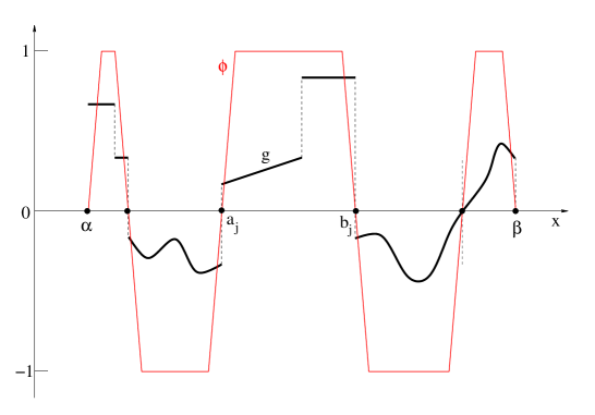
Figure 1: The test function $\phi$ defined at (2.7), with Lipschitz constant $\varepsilon^{-2/3}$.

Lemma 2.1

Let $g:[\alpha,\beta]\mapsto{\mathbb{R}}$ be as above. If $g$ is strictly positive (or strictly negative) for all $x\in[\alpha,\beta]$, then

$$\int_{\alpha+\varepsilon^{2/3}}^{\beta-\varepsilon^{2/3}}|g(x)|\,dx~{}\leq~{}\int_{\alpha}^{\beta}\phi(x)\,g(x)\,dx.$$ (2.8)

On the other hand, if $g(\xi)=0$ for some $\xi\in[\alpha,\beta]$, then

$$\int_{\alpha}^{\beta}|g(x)|\,dx~{}\leq~{}\int_{\alpha}^{\beta}\phi(x)\,g(x)\,dx+2\varepsilon^{2/3}\cdot\hbox{\rm Tot.Var.}\bigl{\{}g\,;~{}[\alpha,\beta]\bigr{\}}.$$ (2.9)

Proof. 1. If $g$ has always the same sign, then by construction $\phi(x)\,g(x)\geq 0$ for all $x$, while $\phi(x)=\hbox{sign}(g(x))$ for $x\in[\alpha+\varepsilon^{2/3},\,\beta-\varepsilon^{2/3}]$. Hence the estimate (2.8) is trivially true. 2. If $g$ changes sign, consider the maximal subintervals $[a_{j},b_{j}]$ where $g$ has a constant sign, as in (G). We then have the estimate

$$\begin{array}[]{l}\displaystyle\int_{\alpha}^{\beta}|g(x)|\,dx~{}=~{}\sum_{j}\int_{a_{j}}^{b_{j}}|g(x)|\,dx\\[11.38109pt] \displaystyle\quad\leq~{}\sum_{b_{j}-a_{j}\leq 2\varepsilon^{2/3}}(b_{j}-a_{j})\sup_{a_{j}<x<b_{j}}|g(x)|\\[11.38109pt] \displaystyle\qquad\qquad\qquad+\sum_{b_{j}-a_{j}\geq 2\varepsilon^{2/3}}\left(\int_{a_{j}+\varepsilon^{2/3}}^{b_{j}-\varepsilon^{2/3}}+\int_{a_{j}}^{a_{j}+\varepsilon^{2/3}}+\int_{b_{j}-\varepsilon^{2/3}}^{b_{j}}\right)|g(x)|\,dx\\[11.38109pt] \displaystyle\quad\leq~{}2\varepsilon^{2/3}\cdot\!\!\!\!\!\sum_{b_{j}-a_{j}\leq 2\varepsilon^{2/3}}\hbox{\rm Tot.Var.}\{g\,;~{}]a_{j},b_{j}]\}+\int_{\alpha}^{\beta}\phi(x)\,g(x)\,dx+2\varepsilon^{2/3}\cdot\!\!\!\!\!\sum_{b_{j}-a_{j}>2\varepsilon^{2/3}}\sup_{a_{j}<x<b_{j}}|g(x)|\\[11.38109pt] \displaystyle\quad=~{}\int_{\alpha}^{\beta}\phi(x)\,g(x)\,dx+2\varepsilon^{2/3}\cdot\hbox{\rm Tot.Var.}\bigl{\{}g\,;~{}[\alpha,\beta]\bigr{\}}.\end{array}$$

MM     

Remark 2.1

Here and in the sequel, one could prove similar results by replacing the exponent $2/3$ with any number $\gamma\in\,]0,1[\,$, and working with test functions which are Lipschitz continuous with constant $\varepsilon^{-\gamma}$. Our choice of $\gamma=2/3$ is motivated by the heuristic expectation that, in most cases, this should yield the sharpest error bounds. See Remark 3.1 for further discussion of this point.

We can now state the main result of this section, providing an error estimate on the trapezoidal domain (2.3).

Lemma 2.2

There exists a constant $C_{1}$ such that the following holds. For a given $\varepsilon>0$, let $u$ be an approximate solution of (1.1) that satisfies the property (P_ε). Let $\Delta$ be the trapezoid in (2.3), and let $w$ be the solution to the linear Cauchy problem (2.4), with $A$ as in (2.1). Then

$$\begin{array}[]{l}\displaystyle\int_{a+\tau\lambda^{+}+\varepsilon^{2/3}}^{b+\tau\lambda^{-}-\varepsilon^{2/3}}\bigl{|}u(\tau,x)-w(\tau,x)\bigr{|}\,dx\\[11.38109pt] \displaystyle\quad\leq~{}C_{1}\bigg{(}\tau\cdot\sup_{(t,x)\in\Delta}\bigl{|}u(t,x)-u(0,\xi)|+\tau\varepsilon^{1/3}+\varepsilon^{2/3}\bigg{)}\cdot\sup_{t\in[0,\tau]}\hbox{\rm Tot.Var.}\bigl{\{}u(t,\cdot)\bigr{\}}.\end{array}$$ (2.10)

Proof. 1. Fix $i\in\{1,\ldots,n\}$. On the interval $[\alpha,\beta]\doteq[a+\tau\lambda^{+},\,b+\tau\lambda^{-}]$, consider the scalar function

$$g_{i}(x)~{}\doteq~{}\ell_{i}\cdot\bigl{[}u(\tau,x)-w(\tau,x)\bigr{]}~{}=~{}\ell_{i}\cdot\bigl{[}u(\tau,x)-u(0,x-\lambda_{i}\tau)\bigr{]}.$$ (2.11)

Let $\phi_{i}:[\alpha,\beta]\mapsto[-1,1]$ be the function with Lipschitz constant $\|\phi_{i}^{\prime}\|_{{\bf L}^{\infty}}=\varepsilon^{-2/3}$, defined as in (2.7) with $g$ replaced by $g_{i}$. We then extend $\phi_{i}$ to the entire real line by setting $\phi_{i}(x)=0$ if $x\notin[\alpha,\beta]$, and consider a test function $\varphi_{i}=\varphi_{i}(t,x)$ such that

$$\varphi_{i}(t,x)~{}=~{}\phi_{i}\bigl{(}x-\lambda_{i}(t-\tau)\bigr{)}\,\ell_{i}\qquad\quad\hbox{for}\quad t\in[0,\tau],~{}x\in{\mathbb{R}}\,.$$ (2.12)

2. Observing that $\lambda_{i}\in[0,1]$ and $\|\varphi_{i}\|_{W^{1,\infty}}=|\ell_{i}|\,\varepsilon^{-2/3}$, by (1.11) we now obtain

$$\begin{array}[]{l}\displaystyle\left|\int\varphi_{i}(0,x)u(0,x)\,dx-\int\varphi_{i}(\tau,x)u(\tau,x)\,dx+\int_{0}^{\tau}\int\bigl{\{}u\varphi_{i,t}+f(u)\varphi_{i,x}\bigr{\}}\,dxdt\right|\\[11.38109pt] \qquad\qquad\displaystyle\leq~{}C\varepsilon\|\varphi_{i}\|_{W^{1,\infty}}\cdot\tau\cdot\sup_{t\in[0,\tau]}\hbox{\rm Tot.Var.}\bigl{\{}u(t,\cdot)\bigr{\}}\\[11.38109pt] \qquad\qquad\displaystyle\leq~{}C^{\prime}\varepsilon^{1/3}\,\tau\cdot\sup_{t\in[0,\tau]}\hbox{\rm Tot.Var.}\bigl{\{}u(t,\cdot)\bigr{\}}.\end{array}$$ (2.13)

3. For future use we observe that, if $x\mapsto u(x)$ is Lipschitz and $u^{*}=u(\xi)$ for some $\xi\in[x_{1},x_{2}]$, then

$$\begin{array}[]{rl}\displaystyle\int_{x_{1}}^{x_{2}}\Big{|}\ell_{i}\bigl{(}f(u)_{x}-\lambda_{i}u_{x}\bigr{)}\Big{|}\,dx&\displaystyle=~{}\int_{x_{1}}^{x_{2}}\Big{|}\ell_{i}\bigl{[}Df(u)-Df(u^{*})\bigr{]}u_{x}\Big{|}\,dx\\[11.38109pt] &\displaystyle\leq~{}C_{0}\,\sup_{x_{1}<x<x_{2}}|u(x)-u^{*}|\cdot\int_{x_{1}}^{x_{2}}|u_{x}|\,dx.\end{array}$$

Here $C_{0}$ is a constant depending only on the function $f$. By an approximation argument, for any BV function $x\mapsto u(x)$ we conclude

$$\hbox{\rm Tot.Var.}\Big{\{}\ell_{i}\bigl{(}f(u)-\lambda_{i}u\bigr{)}\,;~{}[x_{1},x_{2}]\Big{\}}~{}\leq~{}C_{0}\left(\sup_{x_{1}<x<x_{2}}|u(x)-u^{*}|\right)\cdot\hbox{\rm Tot.Var.}\bigl{\{}u\,;~{}[x_{1},x_{2}]\bigr{\}}.$$ (2.14)

4. Since $w$ is a solution to the linear equation (2.4), the choice of the test function $\varphi_{i}$ in (2.12) implies

$$\int\varphi_{i}(0,x)\,u(0,x)\,dx~{}=~{}\int\varphi_{i}(0,x)\,w(0,x)\,dx~{}=~{}\int\varphi_{i}(\tau,x)\,w(\tau,x)\,dx.$$ (2.15)

Moreover, calling $u^{*}=u(0,\xi)$, integrating by parts and using (2.14) together with the bound $\phi_{i}(x)\in[-1,1]$, we obtain

$$\begin{array}[]{l}\displaystyle\left|\int_{0}^{\tau}\int\bigl{\{}u\varphi_{i,t}+f(u)\varphi_{i,x}\bigr{\}}\,dxdt\right|~{}=~{}\left|\int_{0}^{\tau}\int\bigl{[}f(u)-\lambda_{i}u\bigr{]}\,\varphi_{i,x}\,dxdt\right|\\[11.38109pt] \displaystyle\qquad\leq~{}\int_{0}^{\tau}\hbox{\rm Tot.Var.}\Big{\{}\ell_{i}(f(u)-\lambda_{i}u)\,;~{}[a+\lambda^{+}\tau+(t-\tau)\lambda_{i}\,,~{}b+\lambda^{-}\tau+(t-\tau)\lambda_{i}]\Big{\}}\,\|\varphi_{i}\|_{{\bf L}^{\infty}}\,dt\\[11.38109pt] \displaystyle\qquad\leq~{}C_{0}\,\sup_{(t,x)\in\Delta}|u(t,x)-u^{*}|\cdot\int_{0}^{\tau}\hbox{\rm Tot.Var.}\Big{\{}u(t,\cdot)\,;~{}\,]a+t\lambda^{+},\,b+t\lambda^{-}[\Big{\}}\,dt.\end{array}$$ (2.16)

5. By (2.15), combining (2.13) with (2.16) we conclude

$$\begin{array}[]{l}\displaystyle~{}\int_{a+\tau\lambda^{+}}^{b+\tau\lambda^{-}}\phi_{i}(x)\,\ell_{i}\bigl{[}w(\tau,x)-u(\tau,x)\bigr{]}\,dx~{}=~{}\int\varphi_{i}(0,x)u(0,x)\,dx-\int\varphi_{i}(\tau,x)u(\tau,x)\,dx\\[11.38109pt] \qquad\displaystyle\leq~{}\left|\int_{0}^{\tau}\int\bigl{\{}u\varphi_{i,t}+f(u)\varphi_{i,x}\bigr{\}}\,dxdt\right|+{\cal E}_{i}\,,\end{array}$$ (2.17)

where

$$\begin{array}[]{rl}{\cal E}_{i}&\doteq~{}\displaystyle\left|\int\varphi_{i}(0,x)u(0,x)\,dx-\int\varphi_{i}(\tau,x)u(\tau,x)\,dx+\int_{0}^{\tau}\int\bigl{\{}u\varphi_{i,t}+f(u)\varphi_{i,x}\bigr{\}}\,dxdt\right|\\[11.38109pt] &\displaystyle\leq~{}C\varepsilon\|\varphi\|_{W^{1,\infty}}\cdot\tau\cdot\sup_{t\in[0,\tau]}\hbox{\rm Tot.Var.}\bigl{\{}u(t,\cdot)\bigr{\}}.\end{array}$$ (2.18)

Notice that the above inequality follows from (1.11). In addition, the first term on the right hand side of (2.17) is estimated by (2.16). 6. If the function $g_{i}(x)\doteq\ell_{i}\bigl{[}w(\tau,x)-u(\tau,x)\bigr{]}$ always keeps the same sign, we now use (2.8). If it changes sign at least once, we use (2.9). Combining the two cases, by (2.16) and (2.17) we deduce

$$\begin{array}[]{l}\displaystyle\int_{a+\tau\lambda^{+}+\varepsilon^{2/3}}^{b+\tau\lambda^{-}-\varepsilon^{2/3}}\Big{|}\ell_{i}\bigl{[}w(\tau,x)-u(\tau,x)\bigr{]}\Big{|}\,dx\\[11.38109pt] \displaystyle\qquad\leq~{}C_{0}\,\sup_{(t,x)\in\Delta}|u(t,x)-u^{*}|\cdot\int_{0}^{\tau}\hbox{\rm Tot.Var.}\Big{\{}u(t,\cdot)\,;~{}\,]a+t\lambda^{+},\,b+t\lambda^{-}[\Big{\}}\,dt+{\cal E}_{i}\\[11.38109pt] \qquad\qquad\displaystyle+2\varepsilon^{2/3}\cdot\hbox{\rm Tot.Var.}\Big{\{}g_{i}\,;~{}]a+\tau\lambda^{+},b+\tau\lambda^{-}[\Big{\}}.\end{array}$$ (2.19)

7. Recalling (2.5), for any vector $v=\sum_{i}c_{i}r_{i}\in{\mathbb{R}}^{n}$ one has

$$|v|~{}\leq~{}\sum_{i=1}^{n}|c_{i}|~{}=~{}\sum_{i=1}^{n}|\ell_{i}\cdot v|.$$

We use this inequality with $v=w(\tau,x)-u(\tau,x)$. Using (2.11) to compute the total variation of $g_{i}$, summing the inequalities (2.18)-(2.19) for $i=1,\ldots,n$, we obtain

$$\begin{array}[]{l}\displaystyle\int_{a+\tau\lambda^{+}+\varepsilon^{1/3}}^{b+\tau\lambda^{-}-\varepsilon^{1/3}}\Big{|}w(\tau,x)-u(\tau,x)\Big{|}\,dx\\[11.38109pt] \displaystyle\quad\leq~{}nC_{0}\,\sup_{(t,x)\in\Delta}|u(t,x)-u^{*}|\cdot\tau\cdot\sup_{t\in[0,\tau]}\hbox{\rm Tot.Var.}\Big{\{}u(t,\cdot)\,;~{}\,]a+t\lambda^{+},\,b+t\lambda^{-}[\Big{\}}\\[11.38109pt] \displaystyle\qquad+nC\varepsilon\|\varphi\|_{W^{1,\infty}}\cdot\tau\cdot\sup_{t\in[0,\tau]}\hbox{\rm Tot.Var.}\bigl{\{}u(t,\cdot)\bigr{\}}\\[11.38109pt] \displaystyle\qquad+2\varepsilon^{2/3}\left(\sum_{i}|\ell_{i}|\right)\cdot\Big{(}\hbox{\rm Tot.Var.}\bigl{\{}u(0,\cdot)\,;~{}[a,b]\bigr{\}}+\hbox{\rm Tot.Var.}\bigl{\{}u(\tau,\cdot)\,;~{}[a+\tau\lambda^{+},~{}b+\tau\lambda^{-}]\bigr{\}}\Big{)}.\end{array}$$ (2.20)

This yields (2.10), for a suitable constant $C_{1}$. MM     

3 Error bounds for solutions without large shocks

Consider an approximate solution $u=u(t,x)$ of (1.1)-(1.2), constructed by a numerical algorithm with time step $\varepsilon>0$, which satisfies the properties (AL) and (P_ε). We fix a new time step $h>\!>\varepsilon$, and split the interval $[0,T]$ into subintervals $[t_{j},t_{j+1}]$ with $t_{j}=j\,h$. Throughout the following we choose $h\approx\varepsilon^{1/3}$, say

$$c_{0}\varepsilon^{1/3}~{}\leq~{}h~{}\leq~{}\varepsilon^{1/3}$$ (3.1)

for some constant $c_{0}>0$, and assume that both $h$ and $T$ are integer multiples of $\varepsilon$. To simplify the discussion, we also assume that $T=\nu h$ for some integer $\nu$. Notice that, in the general case, one can consider the time $T^{\prime}$ such that

$$T^{\prime}~{}=~{}\nu h~{}\leq~{}T~{}<~{}(\nu+1)h$$

for some integer $\nu$. By (1.10), the difference can then be estimated by

$$\|u(T,\cdot)-u(T^{\prime},\cdot)\|_{{\bf L}^{1}}~{}\leq~{}Lh\cdot\sup_{t\in[0,T]}\hbox{\rm Tot.Var.}\{u(t,\cdot)\}~{}=~{}{\cal O}(1)\cdot\varepsilon^{1/3}.$$

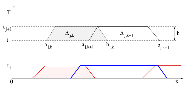
Figure 2: Covering the strip $[0,T]\times{\mathbb{R}}$ with finitely many trapezoids $\Delta_{jk}$.

As shown in Fig. 2, for any given $j=1,2,\ldots,\nu-1$, we cover the real line with finitely many intervals $]a_{jk},b_{jk}[\,$, $k=1,\ldots,N(j)$, so that

$$-\infty~{}=~{}a_{j,1}~{}<~{}a_{j,2}~{}<~{}b_{j,1}~{}<~{}a_{j,3}~{}<~{}\cdots~{}<~{}a_{j,N(j)}~{}<~{}b_{j,N(j)-1}~{}<~{}b_{j,N(j)}~{}=~{}+\infty.$$

We then cover each strip $[t_{j},t_{j+1}]\times{\mathbb{R}}$ with the trapezoids $\Delta_{jk}$, $k=1,\ldots,N(j)$. For convenience, these will be expressed as the convex closure of their four vertices:

$$\Delta_{jk}~{}=~{}\hbox{co}\Big{\{}(t_{j},a_{jk}),~{}~{}(t_{j},b_{jk}),~{}~{}(t_{j+1},a_{jk}+h\lambda^{+}+\varepsilon^{2/3}),~{}~{}(t_{j+1},b_{jk}+h\lambda^{-}-\varepsilon^{2/3})\Big{\}}.$$

Equivalently:

$$\begin{array}[]{l}\Delta_{jk}~{}=~{}\bigg{\{}(t,x)\,;~{}t\in[t_{j},t_{j+1}],\\[11.38109pt] \displaystyle\quad{t_{j+1}-t\over h}a_{jk}+{t-t_{j}\over h}(a_{jk}+h\lambda^{+}+\varepsilon^{2/3})~{}\leq~{}x~{}\leq~{}{t_{j+1}-t\over h}b_{jk}+{t-t_{j}\over h}(b_{jk}+h\lambda^{-}-\varepsilon^{2/3})\bigg{\}}.\end{array}$$ (3.2)

By suitably choosing the points $a_{jk}$, $b_{jk}$, we can assume that the intervals

$$J_{jk}^{\prime}~{}=~{}[a_{jk}+h\lambda^{+}+\varepsilon^{2/3}\,,~{}b_{jk}+h\lambda^{-}-\varepsilon^{2/3}],\qquad k=1,\ldots,N(j),$$

form a partition of ${\mathbb{R}}$. Namely

$$b_{jk}+h\lambda^{-}-\varepsilon^{2/3}~{}=~{}a_{j,k+1}+h\lambda^{+}+\varepsilon^{2/3},\qquad\quad k=1,\ldots,N(j)-1.$$ (3.3)

Furthermore, by choosing the bases of all trapezoids to have length

$$b_{jk}-a_{jk}~{}>~{}2h(\lambda^{+}-\lambda^{-}),$$ (3.4)

we can assume that each point $(t,x)\in[t_{j},t_{j+1}]\times{\mathbb{R}}$ is contained in at least one and in not more than two of these trapezoids.

Next, we recall that the oscillation of $u$ over a set $\Delta$ is defined as

$$\hbox{\rm Osc.}\bigl{\{}u\,;~{}\Delta\bigr{\}}~{}\doteq~{}\sup_{(t,x),(s,y)\in\Delta}~{}|u(t,x)-u(t,y)|.$$

For each fixed $j\in\{1,\ldots,\nu\}$, the maximum oscillation of $u$ over all trapezoids $\Delta_{jk}$ will be denoted by

$$\kappa_{j}~{}\doteq~{}\max_{1\leq k\leq N(j)}\hbox{\rm Osc.}\bigl{\{}u\,;~{}\Delta_{jk}\bigr{\}}\,.$$ (3.5)

Let now $S:[0,+\infty[\,\times{\cal D}\mapsto{\cal D}$ be the Lipschitz semigroup generated by the hyperbolic system (1.1), as in (1.6)-(1.7). In particular, $t\mapsto S_{t}\bar{u}$ yields the exact solution to the Cauchy problem (1.1)-(1.2). As proved in [7, 8], for any approximate solution $u$ one has the error estimate

$$\|u(T,\cdot)-S_{T}\bar{u}\|_{{\bf L}^{1}}~{}\leq~{}L_{0}\cdot\sum_{j=0}^{\nu-1}\Big{\|}u(t_{j+1},\cdot)-S_{h}u(t_{j},\cdot)\Big{\|}_{{\bf L}^{1}}\,.$$ (3.6)

For each $j$, we will show that the corresponding term on the right hand side of (3.6) can be estimated using (2.10).

Consider the covering of the strip $[t_{j},t_{j+1}]\times{\mathbb{R}}$ in terms of the trapezoids $\Delta_{jk}$, introduced at (3.2). As in (2.4), for $k=1,\ldots,N(j)$ we shall denote by $w^{(k)}$ the solution to the linearized problem with constant coefficients

$$w_{t}+Aw_{x}~{}=~{}0,\qquad\quad w(t_{j},\cdot)=u(t_{j},\cdot),\qquad\quad A\doteq Df\bigl{(}u(t_{j},\xi_{k})\bigr{)},$$ (3.7)

for some given points $\xi_{k}\in\,]a_{jk},\,b_{jk}\,[$.

Let $\ell_{i}^{(k)}$ be the $i$-th left eigenvector of the above matrix $A$, normalized as in (2.5). Using (2.19) on each trapezoid $\Delta_{jk}$ we obtain

$$\begin{array}[]{l}\displaystyle\int_{a_{jk}+h_{j}\lambda^{+}+\varepsilon^{2/3}}^{b_{jk}+h_{j}\lambda^{-}-\varepsilon^{2/3}}\left|\ell_{i}^{(k)}\cdot\bigl{[}u(t_{j+1},x)-w^{(k)}(t_{j+1},x)\bigr{]}\right|\,dx\\[11.38109pt] \displaystyle\leq~{}C_{0}\cdot\hbox{\rm Osc.}\{u\,;~{}\Delta_{jk}\}\cdot\int_{t_{j}}^{t_{j+1}}\hbox{\rm Tot.Var.}\Big{\{}u(t,\cdot)\,;~{}]a_{jk}+(t-t_{j})\lambda^{+},b_{jk}+(t-t_{j})\lambda^{-}[\Big{\}}\,dt\\[11.38109pt] \quad\displaystyle+\left|\int\varphi_{i}^{(k)}(t_{j},x)u(t_{j},x)\,dx-\int\varphi_{i}^{(k)}(t_{j+1},x)u(t_{j+1},x)\,dx+\int\!\!\!\int_{\Delta_{jk}}\left\{u\varphi^{(k)}_{i,t}+f(u)\varphi^{(k)}_{i,x}\right\}\,dxdt\right|\\[11.38109pt] \quad+2\varepsilon^{2/3}\cdot\hbox{\rm Tot.Var.}\Big{\{}\ell_{i}\cdot u(t_{j},\cdot)\,;~{}[a_{jk},b_{jk}]\Big{\}}\\[11.38109pt] \quad+2\varepsilon^{2/3}\cdot\hbox{\rm Tot.Var.}\Big{\{}\ell_{i}\cdot u(t_{j+1},\cdot)\,;~{}[a_{jk}+h_{j}\lambda^{+}\,,~{}b_{jk}+h_{j}\lambda^{-}]\Big{\}}\bigg{)}\\[11.38109pt] \doteq~{}A_{ik}+B_{ik}+C_{ik}+D_{ik}\,.\end{array}$$ (3.8)

For notational convenience, call $\chi_{jk}$ the characteristic function of the interval $[a_{jk}+h_{j}\lambda^{+}+\varepsilon^{2/3}\,,~{}b_{jk}+h_{j}\lambda^{-}-\varepsilon^{2/3}]$. Our next goal is to estimate the quantity

$$E_{j}~{}\doteq~{}\int_{-\infty}^{+\infty}\left|u(t_{j+1},x)-\sum_{k}w^{(k)}(t_{j+1},x)\cdot\chi_{jk}(x)\right|\,dx\,.$$ (3.9)

This can of course be achieved by summing the terms on the right hand side of (3.8) over all $i=1,\ldots,n$ and $k=1,\ldots,N(j)$. Toward this goal, we recall the key assumption that every point $(t,x)\in[t_{j},t_{j+1}]\times{\mathbb{R}}$ belongs to one and no more than two of the trapezoids $\Delta_{jk}$. More precisely, we have the implication

$$|k-k^{\prime}|\,\geq\,2\qquad\Longrightarrow\qquad\Delta_{jk}\cap\Delta_{jk^{\prime}}~{}=~{}\emptyset.$$ (3.10)

Recalling (3.5), for a fixed $i$ we thus obtain

$$\sum_{k=1}^{N(j)}A_{ik}~{}\leq~{}C_{0}\,\kappa_{j}\cdot\int_{t_{j}}^{t_{j+1}}2\,\hbox{\rm Tot.Var.}\{u(t,\cdot)\}\,dt.$$ (3.11)

$$\sum_{k=1}^{N(j)}C_{ik}~{}\leq~{}4\varepsilon^{2/3}\,\hbox{\rm Tot.Var.}\{u(t_{j},\cdot)\},\qquad\qquad\sum_{k=1}^{N(j)}D_{ik}~{}\leq~{}4\varepsilon^{2/3}\,\hbox{\rm Tot.Var.}\{u(t_{j+1},\cdot)\}.$$ (3.12)

The estimate for $\sum_{k}B_{jk}$ is a bit more delicate, because if we use (1.11) separately on each subdomain $\Delta_{jk}$, the error term on the right side would be multiplied by $N(j)$, which can be a very large number.

For this reason, we argue as follows. For each $i\in\{1,\ldots,n\}$, we consider test functions $\varphi$, $\widetilde{\varphi}_{i}$ which satisfy, for $t\in[t_{j},t_{j+1}]$,

$$\varphi_{i}(t,x)~{}=~{}\left\{\begin{array}[]{cl}\varphi^{(k)}_{i}(t,x)&\hbox{if}~{}~{}(t,x)\in\Delta_{jk}\,,~{}~{}k~{}\hbox{even},\cr 0&\hbox{otherwise.}\end{array}\right.$$

$$\widetilde{\varphi}_{i}(t,x)~{}=~{}\left\{\begin{array}[]{cl}\varphi^{(k)}_{i}(t,x)&\hbox{if}~{}~{}(t,x)\in\Delta_{jk}\,,~{}~{}k~{}\hbox{odd},\cr 0&\hbox{otherwise.}\end{array}\right.$$

For convenience, we denote by $\ell_{\rm max}$ an upper bound for the norm of all left eigenvectors $\ell_{i}=\ell_{i}(u)$ of all matrices $A(u)=Df(u)$, normalized as in (2.5). With this notation we have

$$\|\varphi_{i}\|_{W^{1\infty}}~{}\leq~{}\ell_{\rm max}\cdot\varepsilon^{-2/3}\,,\qquad\qquad\|\widetilde{\varphi}_{i}\|_{W^{1\infty}}~{}\leq~{}\ell_{\rm max}\cdot\varepsilon^{-2/3}.$$ (3.13)

Applying (1.11) to the test function $\varphi_{i}$, then to $\widetilde{\varphi}_{i}$, we obtain

$$\sum_{k~{}{\rm even}}~{}B_{ik}~{}\leq~{}C\varepsilon h\,\varepsilon^{-2/3}\ell_{\rm max}\cdot\sup_{t\in[t_{j},t_{j+1}]}\hbox{\rm Tot.Var.}\bigl{\{}u(t,\cdot)\big{\}},$$

$$\sum_{k~{}{\rm odd}}~{}B_{ik}~{}\leq~{}C\varepsilon h\,\varepsilon^{-2/3}\ell_{\rm max}\cdot\sup_{t\in[t_{j},t_{j+1}]}\hbox{\rm Tot.Var.}\bigl{\{}u(t,\cdot)\big{\}}.$$

Summing over $k$, we thus obtain

$$\sum_{k=1}^{N(j)}B_{ik}~{}\leq~{}2Ch\varepsilon^{1/3}\ell_{\rm max}\cdot\sup_{t\in[t_{j},t_{j+1}]}\hbox{\rm Tot.Var.}\bigl{\{}u(t,\cdot)\big{\}}.$$ (3.14)

All together, the inequalities (3.11), (3.12), and (3.14) yield

$$\begin{array}[]{l}\displaystyle\int_{-\infty}^{+\infty}\left|u(t_{j+1},x)-\sum_{k}w^{(k)}(t_{j+1},x)\cdot\chi_{jk}(x)\right|\,dx\\[11.38109pt] \qquad\displaystyle\leq~{}C_{0}\,2n\kappa_{j}\int_{t_{j}}^{t_{j+1}}\hbox{\rm Tot.Var.}\bigl{\{}u(t,\cdot)\bigr{\}}\,dt+4n\varepsilon^{2/3}\hbox{\rm Tot.Var.}\bigl{\{}u(t_{j},\cdot)\bigr{\}}\\[11.38109pt] \qquad\qquad+\displaystyle 4n\varepsilon^{2/3}\hbox{\rm Tot.Var.}\bigl{\{}u(t_{j+1},\cdot)\bigr{\}}+2Ch\,\varepsilon^{1/3}\ell_{\rm max}\cdot\sup_{t\in[t_{j},t_{j+1}]}\hbox{\rm Tot.Var.}\bigl{\{}u(t,\cdot)\big{\}}.\end{array}$$ (3.15)

Next, we replace the approximate solution $u$ with the exact solution $u^{exact}(t_{j}+s,\cdot)~{}=~{}S_{s}u(t_{j},\cdot)$ of (1.1) having the same data at $t=t_{j}$. As proved in [7], with the same notation used in (3.9), as long as $u(t_{j},\cdot)\in{\cal D}$ remains in the domain of the semigroup, one has

$$\begin{array}[]{l}\displaystyle\int_{-\infty}^{+\infty}\left|u^{exact}(t_{j+1},x)-\sum_{k}w^{(k)}(t_{j+1},x)\cdot\chi_{jk}(x)\right|\,dx\\[11.38109pt] \qquad\displaystyle\leq~{}C_{2}\,h\left(\max_{1\leq k\leq N(j)}\hbox{\rm Osc.}\left\{u(t_{j},\cdot)\,;~{}\Delta_{jk}\,\right\}\right)\cdot\hbox{\rm Tot.Var.}\bigl{\{}u(t_{j},\cdot)\bigr{\}},\end{array}$$ (3.16)

for a suitable constant $C_{2}$.

Combining (3.15) with (3.16) and recalling (3.5), we obtain

$$\begin{array}[]{l}\displaystyle\int_{-\infty}^{+\infty}\Big{|}u(t_{j+1},x)-\bigl{(}S_{t_{j+1}-t_{j}}u(t_{j},\cdot)\bigr{)}(x)\Big{|}\,dx\\[11.38109pt] \qquad\displaystyle\leq~{}C_{3}\left(\kappa_{j}\,h+\varepsilon^{2/3}+h\varepsilon^{1/3}\right)\cdot\sup_{t\in[t_{j},t_{j+1}]}\hbox{\rm Tot.Var.}\bigl{\{}u(t,\cdot)\bigr{\}}.\end{array}$$ (3.17)

Recalling that $h\approx\varepsilon^{1/3}$ and $T=\nu\varepsilon^{1/3}$, from the above analysis we obtain:

Theorem 3.1

Let the basic assumptions (A1)-(A2) hold. Let $t\mapsto u(t,\cdot)\in{\cal D}$ be an approximate solution to the Cauchy problem (1.1)-(1.2), taking values in the domain ${\cal D}$ of the semigroup and satisfying (AL) and (P_ε). Then, for some constant $C_{4}$, the following holds.

Assume that the strip $[0,T]\times{\mathbb{R}}$ can be covered by trapezoids $\Delta_{jk}$, $j=0,\ldots,\nu-1$, $k=1,\ldots N(j)$ as in (3.2), so that (3.3)-(3.5) hold. Then the difference between $u(T,\cdot)$ and the exact solution $S_{T}\bar{u}$ is bounded by

$$\|u(T,\cdot)-S_{T}\bar{u}\|_{{\bf L}^{1}}~{}\leq~{}C_{4}\left(2T+\sum_{j=0}^{\nu-1}\kappa_{j}\right)\varepsilon^{1/3}\cdot\sup_{t\in[0,T]}\hbox{\rm Tot.Var.}\bigl{\{}u(t,\cdot)\bigr{\}}\,.$$ (3.18)

Proof. Let $L_{0}$ be the Lipschitz constant of the semigroup in (1.7). From (3.6) and (3.17) it now follows

$$\begin{array}[]{l}\displaystyle\|u(T,\cdot)-S_{T}\bar{u}\|_{{\bf L}^{1}}~{}\leq~{}L_{0}\cdot\sum_{j=0}^{\nu-1}\Big{\|}u(t_{j+1},\cdot)-S_{h}u(t_{j},\cdot)\Big{\|}_{{\bf L}^{1}}\\[11.38109pt] \qquad\displaystyle\leq~{}L_{0}\cdot\sum_{j=0}^{\nu-1}C_{3}\left(\kappa_{j}\,h+\varepsilon^{2/3}+h\varepsilon^{1/3}\right)\cdot\sup_{t\in[t_{j},t_{j+1}]}\hbox{\rm Tot.Var.}\bigl{\{}u(t,\cdot)\bigr{\}}\\[11.38109pt] .\qquad\displaystyle\leq~{}L_{0}\,C_{3}\cdot\left(2T+\sum_{j=0}^{\nu-1}\kappa_{j}\right)\varepsilon^{1/3}\cdot\sup_{t\in[0,T]}\hbox{\rm Tot.Var.}\bigl{\{}u(t,\cdot)\bigr{\}}.\end{array}$$ (3.19)

This yields (3.18), with $C_{4}=L_{0}C_{3}$. MM     

Remark 3.1

Based on the estimate (3.19), we seek to understand at which rate the error in the approximate solution may approach zero, as $\varepsilon\to 0$.

Having chosen $h\approx\varepsilon^{1/3}$, we can choose all bounded trapezoids $\Delta_{jk}$, $1<k<N(j)$, to be of diameter ${\cal O}(1)\cdot\varepsilon^{1/3}$. Moreover, by choosing every $b_{j1}$ suitably large and negative, and $a_{j,N(j)}$ large and positive, we can assume that the solution is nearly constant on the unbounded trapezoids $\Delta_{j,1}$ and $\Delta_{j,N(j)}$. Here and in the sequel, the Landau symbol ${\cal O}(1)$ denotes a uniformly bounded quantity.

If the exact solution is Lipschitz continuous, we expect that the maximum oscillation (3.5) will be of size $\kappa_{j}={\cal O}(1)\cdot\varepsilon^{1/3}$ for every $j\in\{0,1,\ldots,\nu-1\}$. In this case, as $\varepsilon\to 0$ the quantity $2T+\sum_{j=1}^{\nu}\kappa_{j}$ remains uniformly bounded, and the estimate (3.19) indicates that the error vanishes of order ${\cal O}(1)\cdot\varepsilon^{1/3}$.

Next, assume that the initial data $\bar{u}$ contains a jump, generating a centered rarefaction wave of strength $\sigma$. In this case, taking into account the decay caused by genuine nonlinearity, we expect that the oscillation of $u$ over a trapezoid $\Delta_{jk}$ of diameter ${\cal O}(1)\cdot\varepsilon^{1/3}$ will satisfy a bound of the form

$$\hbox{\rm Osc.}\left\{u(t,\cdot)\,;~{}\Delta_{jk}\right\}~{}=~{}{\cal O}(1)\cdot\min\left\{\sigma\,,~{}{\varepsilon^{1/3}\over t_{j}}\right\}.$$ (3.20)

Recalling that $t_{j}=j\varepsilon^{1/3}$ and $\nu=T\varepsilon^{-1/3}$, this leads to

$$\sum_{j=1}^{\nu}\kappa_{j}~{}=~{}\sum_{j=1}^{\nu}\min\left\{\sigma\,,~{}{C\varepsilon^{1/3}\over j\varepsilon^{1/3}}\right\}~{}=~{}{\cal O}(1)\cdot\log\nu~{}=~{}{\cal O}(1)\cdot|\log\varepsilon|.$$ (3.21)

In this case, the estimate (3.19) would indicate that the error vanishes of order ${\cal O}(1)\cdot\varepsilon^{1/3}\,|\log\varepsilon|$. The same should hold if the exact solution contains finitely many centered rarefaction waves.

We emphasize, however, that this is only a heuristic expectation. For a numerically computed solution, it needs to be confirmed by a post-processing algorithm, which can actually provide a bound on the oscillations $\kappa_{j}$ in (3.18).

4 Solutions with an isolated large shock

The error estimates developed in the previous section are not effective for solutions containing large shocks. Indeed, around a shock, the oscillation will be large. As a consequence, even when the diameters of the trapezoids $\Delta_{jk}$ in (3.2) approach zero, the maximum oscillation $\kappa_{j}$ in (3.5) will remain uniformly large. For this reason, we do not expect that the right hand side of the error bound (3.18) will approach zero as $\varepsilon\to 0$. To cope with this problem, in this section we develop additional tools to estimate the numerical error in a neighborhood of a shock.

Figure 3: The regions $\Gamma_{l},\Gamma_{m},\Gamma_{r}$ introduced at (4.13) to trace a large shock, and the trapezoid $\Delta^{\prime}$ at (4.4).

Consider an approximate solution $u$, which satisfies (AL) and (P_ε). We seek a sharper error bound, assuming that the oscillation of $u$ is concentrated in a narrow region of the form

$$\Gamma~{}\doteq~{}\Big{\{}(t,x)\,;~{}t\in[0,h],~{}|x-\gamma(t)|<\delta\Big{\}},\qquad\qquad\gamma(t)=x_{0}+\lambda t.$$ (4.1)

Of course, we expect that $\gamma(\cdot)$ will trace the position of a large shock in the exact solution. Here $\rho,\delta>0$ are suitable parameters. Different choices of these values will lead to different estimates. As a rule of thumb, it will be useful for the reader to keep in mind their order of magnitude:

$$h\,\approx\,\varepsilon^{1/3},\qquad\rho\,\approx\,\varepsilon^{1/3},\qquad\delta\,\approx\,{\varepsilon\over\rho}\,~{}=~{}\varepsilon^{2/3}.$$ (4.2)

Referring to Fig. 3, we introduce the points

$$\left\{\begin{array}[]{rl}a&=~{}x_{0}+\lambda^{-}h-\delta-\rho,\\[8.53581pt] b&=~{}x_{0}+\lambda^{+}h+\delta+\rho,\end{array}\right.\qquad\qquad\left\{\begin{array}[]{rl}a^{\prime}&\doteq~{}a-\lambda^{+}h,\\[8.53581pt] b^{\prime}&\doteq~{}b-\lambda^{-}h,\end{array}\right.$$ (4.3)

and consider the trapezoidal domain

$$\begin{array}[]{rl}\Delta^{\prime}&\doteq~{}\hbox{co}\Big{\{}(0,a^{\prime}),\,(0,b^{\prime}),\,(h,a),\,(h,b)\Big{\}}\\[8.53581pt] &=~{}\Big{\{}(t,x)\,;~{}t\in[0,h]\,,~{}~{}a^{\prime}+\lambda^{+}t\,\leq\,x\,\leq\,b^{\prime}+\lambda^{-}t\Big{\}}.\end{array}$$ (4.4)

Our basic assumption is that, outside the narrow strip $\Gamma$, the oscillation of $u$ remains small. More precisely, consider the left and right domains

$$\begin{array}[]{rl}\Delta^{\prime}_{l}&=~{}\Big{\{}(t,x)\,;~{}t\in[0,h]\,,~{}~{}a^{\prime}+\lambda^{+}t\,\leq\,x\,\leq\,x_{0}-\delta+\lambda t\Big{\}},\\[8.53581pt] \Delta^{\prime}_{r}&=~{}\Big{\{}(t,x)\,;~{}t\in[0,h]\,,~{}~{}x_{0}+\delta+\lambda t\,\leq\,x\,\leq\,b^{\prime}+\lambda^{-}t\Big{\}},\end{array}$$ (4.5)

and define

$$\kappa^{\prime}~{}\doteq~{}\max\Big{\{}\hbox{\rm Osc.}\{u\,;~{}\Delta^{\prime}_{l}\}\,,~{}\hbox{\rm Osc.}\{u\,;~{}\Delta^{\prime}_{r}\}\Big{\}}.$$ (4.6)

Calling

$$u^{-}~{}\doteq~{}u\bigl{(}0,x_{0}-\delta\bigr{)},\qquad u^{+}~{}\doteq~{}u\bigl{(}0,x_{0}+\delta\bigr{)},$$ (4.7)

the above definition of $\kappa^{\prime}$ implies

$$\begin{array}[]{rl}|u(t,x)-u^{-}|~{}\leq~{}\kappa^{\prime}&\hbox{for}\quad(t,x)\in\Delta^{\prime}_{l}\,,\\[8.53581pt] |u(t,x)-u^{+}|~{}\leq~{}\kappa^{\prime}&\hbox{for}\quad(t,x)\in\Delta^{\prime}_{r}\,.\end{array}$$ (4.8)

Assuming that $\kappa^{\prime}$ is small, the following result provides a bound on the distance between $u$ and the exact solution, $\|u(h,\cdot)-S_{h}\bar{u}\|_{{\bf L}^{1}([a,b])}$, restricted to the interval $[a,b]$.

Theorem 4.1

Let $t\mapsto u(t,\cdot)\in{\cal D}$ be an approximate solution to the Cauchy problem (1.1)-(1.2), taking values in the domain ${\cal D}$ of the semigroup, and satisfying (AL) and (P_ε). Then, for some constant $C_{5}$, in the above setting we have the error bound

$$\int_{a}^{b}\bigl{|}u(h,x)-(S_{h}\bar{u})(x)\bigr{|}\,dx~{}\leq~{}C_{5}\cdot h\,\left({\varepsilon\over\rho}+\kappa^{\prime}+{\rho\kappa^{\prime}+\delta\over h}\right)^{2/3}+C_{5}\,\Big{(}\rho\kappa^{\prime}+h\kappa^{\prime}+\delta\Big{)}.$$ (4.9)

Moreover, there exists a constant $K_{1}$ such that, if

$$|u^{+}-u^{-}|~{}\geq~{}K_{1}\cdot\left({\varepsilon\over\delta}+\kappa^{\prime}+{\rho\kappa^{\prime}+\delta\over h}\right)^{1/3},$$ (4.10)

then the estimate (4.9) can be improved to

$$\int_{a}^{b}\bigl{|}u(h,x)-(S_{h}\bar{u})(x)\bigr{|}\,dx~{}\leq~{}C_{5}\cdot h\,\left({\varepsilon\over\rho}+\kappa^{\prime}+{\rho\kappa^{\prime}+\delta\over h}\right).$$ (4.11)

Remark 4.1

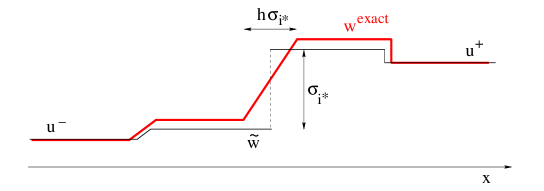
Figure 4: Comparing the entropic solution $w^{exact}$ to the Riemann problem with left and right states $u^{-},u^{+}$ with another weak solution $\widetilde{w}$ containing a non-admissible $i^{*}$-shock of strength $\sigma_{i^{*}}>0$. Taking into account the presence of a centered rarefaction wave in $w^{exact}$, The difference between the two solutions can be bounded as $\|\widetilde{w}(h,\cdot)-w^{exact}(h,\cdot)\|_{{\bf L}^{1}}={\cal O}(1)\cdot h\sigma_{i^{*}}^{2}$.

It may seem surprising that the error bound (4.11), valid for large jumps, is actually better than (4.9), which applies to small jumps. To understand what is involved here, the following observation can be useful. If the strength $\sigma=|u^{+}-u^{-}|$ is small, it could be that this jump is tracing a centered rarefaction wave within the exact solution, which gets approximated by a single jump by the numerical algorithm (indeed, this is a common feature of front tracking approximations). If $\sigma$ is small enough, the entropy produced by the jump is small, and the assumptions (1.11)-(1.12) can still be satisfied. This is a “worst-case scenario”: as shown in Fig. 4, the corresponding ${\bf L}^{1}$ error is ${\cal O}(1)\cdot h\sigma^{2}$. On the other hand, if the strength $\sigma$ of the jump is large, the entropy dissipation assumption (1.12) rules out this possibility. Therefore, the jump must trace an entropic shock in the exact solution.

Proof of Theorem 4.1.

1. As a first step, using (P_ε) we will provide a bound for the error

$$\Big{|}f(u^{+})-f(u^{-})-\lambda\bigl{(}u^{+}-u^{-}\bigr{)}\Big{|}.$$ (4.12)

As shown in Fig. 3, denote by $\Gamma_{l}$, $\Gamma_{m}$, and $\Gamma_{r}$ the left, middle, and right domains

$$\begin{array}[]{rl}\Gamma_{l}&\doteq~{}\bigl{\{}(t,x)\,;~{}t\in[0,h],~{}~{}x\in[\gamma(t)-\delta-\rho\,,~{}\gamma(t)-\delta]\bigr{\}},\\[8.53581pt] \Gamma_{m}&\doteq~{}\bigl{\{}(t,x)\,;~{}t\in[0,h],~{}~{}x\in[\gamma(t)-\delta\,,~{}\gamma(t)+\delta]\bigr{\}},\\[8.53581pt] \Gamma_{r}&\doteq~{}\bigl{\{}(t,x)\,;~{}t\in[0,h],~{}~{}x\in[\gamma(t)+\delta\,,~{}\gamma(t)+\delta+\rho]\bigr{\}}.\end{array}$$ (4.13)

Recalling (4.1), (4.3) and (4.4), we observe that the above definitions imply

$$\Gamma_{m}~{}=~{}\Gamma,\qquad\qquad\Gamma_{l}\cup\Gamma_{m}\cup\Gamma_{r}~{}\subset~{}\Delta^{\prime}.$$

Given $\rho>0$, consider a Lipschitz test function $\varphi$ such that, for $t\in[0,h]$, one has

$$\phi(t,x)~{}=~{}\left\{\begin{array}[]{cl}0&\hbox{if}\quad|x-\gamma(t)|~{}\geq~{}\delta+\rho,\\[8.53581pt] 1&\hbox{if}\quad|x-\gamma(t)|~{}\leq~{}\delta,\\[8.53581pt] \displaystyle{\delta+\rho-|x-\gamma(t)|\over\rho}&\hbox{if}\quad\delta<|x-\gamma(t)|<\delta+\rho.\end{array}\right.$$ (4.14)

Then choose any unit vector ${\bf w}\in{\mathbb{R}}^{n}$ and set $\varphi(t,x)=\phi(t,x)\,{\bf w}$. By construction, for $t\in[0,h]$ the test function $\varphi$ vanishes outside the union $\Gamma_{l}\cup\Gamma_{m}\cup\Gamma_{r}$. Notice that

$$\|\varphi_{x}\|_{{\bf L}^{\infty}}~{}=~{}{1\over\rho}\,,\qquad\qquad\|\varphi_{t}\|_{{\bf L}^{\infty}}~{}=~{}{|\lambda|\over\rho}\,.$$

Assuming that the approximate solution $u$ satisfies ($\bf P_{\varepsilon}$), by (1.11) it follows

$$\begin{array}[]{l}\displaystyle\left|\int\varphi(0,x)u(0,x)\,dx-\int\varphi(h,x)u(h,x)\,dx+\int\!\!\!\int_{\Gamma_{l}\cup\Gamma_{m}\cup\Gamma_{r}}u\varphi_{t}+f(u)\varphi_{x}~{}dxdt\right|\\[11.38109pt] \displaystyle\qquad\leq~{}C\,\varepsilon\,h\cdot{\max\bigl{\{}1,\,|\lambda|\bigr{\}}\over\rho}\cdot\sup_{t\in[0,h]}\hbox{\rm Tot.Var.}\bigl{\{}u(t,\cdot)\bigr{\}}\,.\end{array}$$ (4.15)

Using (4.8), we now estimate

$$\left(\int\!\!\!\int_{\Gamma_{l}}+\int\!\!\!\int_{\Gamma_{m}}+\int\!\!\!\int_{\Gamma_{r}}\right)\bigl{\{}u\varphi_{t}+f(u)\varphi_{x}\bigr{\}}~{}dx\,dt~{}\doteq~{}{\bf I}_{l}+{\bf I}_{m}+{\bf I}_{r}\,.$$ (4.16)

Trivially, ${\bf I}_{m}=0$ because $\varphi_{t}=\varphi_{x}=0$ on $\Gamma_{m}$. By (4.8) it follows

$$\begin{array}[]{rl}\displaystyle{\bf I}_{r}+{\bf I}_{l}&=\displaystyle~{}\int\!\!\!\int_{\Gamma_{r}\cup\Gamma_{l}}\bigl{\{}u\varphi_{t}+f(u)\varphi_{x}\bigr{\}}~{}dxdt\\[11.38109pt] &=~{}\displaystyle\int_{0}^{h}\Big{\{}\bigl{[}\lambda u^{+}-f(u^{+})\bigr{]}-\bigl{[}\lambda u^{-}-f(u^{-})\bigr{]}\Big{\}}{\bf w}\,dt+{\cal O}(1)\cdot h\,\kappa^{\prime}.\end{array}$$ (4.17)

Next, by (4.6) one obtains

$$\begin{array}[]{l}\displaystyle\left|\int\varphi(0,x)u(0,x)\,dx-\int\varphi(h,x)u(h,x)\,dx\right|\\[11.38109pt] \displaystyle\leq~{}\left(\int_{x_{0}-\delta-\rho}^{x_{0}-\delta}+\int_{x_{0}+\delta}^{x_{0}+\delta+\rho}\right)\Big{|}u(0,x)-u(h,x+\lambda h)\Big{|}\,dx+\int_{x_{0}-\delta}^{x_{0}+\delta}\Big{(}|u(0,x)|+|u(h,x+\lambda h)|\Big{)}\,dx\\[11.38109pt] \displaystyle\leq~{}\rho\cdot\hbox{\rm Osc.}\{u\,;~{}\Delta^{\prime}_{l}\}+\rho\cdot\hbox{\rm Osc.}\{u\,;~{}\Delta^{\prime}_{r}\}+2\delta\cdot 2\|u\|_{{\bf L}^{\infty}}~{}\leq~{}2\rho\kappa^{\prime}+4\delta\,\|u\|_{{\bf L}^{\infty}}\,.\end{array}$$ (4.18)

From (4.15), by (4.17) and (4.18) it follows

$$\begin{array}[]{l}\displaystyle\left|\int_{0}^{h}\Big{\{}\lambda(u^{+}-u^{-})-\bigl{[}f(u^{+})-f(u^{-})\bigr{]}\Big{\}}{\bf w}\,dt\right|~{}=~{}{\cal O}(1)\cdot\left({\varepsilon\,h\over\rho}+h\kappa^{\prime}+\rho\kappa^{\prime}+\delta\right),\end{array}$$ (4.19)

where the factor ${\cal O}(1)$ already accounts for the uniform bound on the total variation. Choosing the unit vector

$${\bf w}~{}=~{}{\lambda(u^{+}-u^{-})-\bigl{[}f(u^{+})-f(u^{-})\bigr{]}\over\Big{|}\lambda(u^{+}-u^{-})-\bigl{[}f(u^{+})-f(u^{-})\bigr{]}\Big{|}}\,,$$

by (4.19) we conclude that the error in the Rankine-Hugoniot equations has size

$$\Big{|}\lambda(u^{+}-u^{-})-\bigl{[}f(u^{+})-f(u^{-})\bigr{]}\Big{|}~{}=~{}{\cal O}(1)\cdot\left({\varepsilon h\over\rho}+h\kappa^{\prime}+{\rho\kappa^{\prime}+\delta\over h}\right).$$ (4.20)

2. Next, consider the piecewise constant function

$$w(t,x)~{}\doteq~{}\left\{\begin{array}[]{rl}u^{-}\quad\hbox{if}\quad x<x_{0}+\lambda t,\\[8.53581pt] u^{+}\quad\hbox{if}\quad x>x_{0}+\lambda t.\end{array}\right.$$ (4.21)

Aim of the next two steps is to prove that the difference between $w$ and an exact solution having the same initial data is bounded by

$$\|w(h,\cdot)-S_{h}w(0,\cdot)\|_{{\bf L}^{1}({\mathbb{R}})}~{}=~{}{\cal O}(1)\cdot h\,\Big{|}\lambda(u^{+}-u^{-})-\bigl{[}f(u^{+})-f(u^{-})\bigr{]}\Big{|}.$$ (4.22)

With this goal in mind, define the averaged Jacobian matrix

$$A~{}=~{}\int_{0}^{1}Df\bigl{(}su^{+}+(1-s)u^{-}\bigr{)}\,ds.$$

Call $\lambda_{1}<\cdots<\lambda_{n}$ the eigenvalues of $A$. Let $\{r_{1},\ldots,r_{n}\}$ and $\{\ell_{1},\ldots,\ell_{n}\}$ be dual bases of right and left eigenvectors of $A$, normalized as (2.5). Moreover, let $c_{i}$, $\ell_{max}$ be such that

$$u^{+}-u^{-}~{}=~{}\sum_{i=1}^{n}c_{i}r_{i}\,,\qquad\qquad\ell_{max}~{}\doteq~{}\max\{|\ell_{1}|,\ldots,|\ell_{n}|\}.$$ (4.23)

For every $i=1,\ldots,n$, we then have

$$\Big{|}\ell_{i}\cdot(\lambda I-A)(u^{+}-u^{-})\Big{|}~{}=~{}|c_{i}|\,|\lambda-\lambda_{i}|~{}\leq~{}\ell_{max}\Big{|}\lambda(u^{+}-u^{-})-\bigl{[}f(u^{+})-f(u^{-})\bigr{]}\Big{|}.$$ (4.24)

Let $i^{*}\in\{1,\ldots,n\}$ be a characteristic family such that $|\lambda-\lambda_{i^{*}}|=\min_{i}|\lambda-\lambda_{i}|$. Since the eigenvalues of $A$ are strictly separated, by (4.24) it follows

$$|c_{i}|~{}=~{}{\cal O}(1)\cdot\Big{|}\lambda(u^{+}-u^{-})-\bigl{[}f(u^{+})-f(u^{-})\bigr{]}\Big{|}\qquad\hbox{for all}~{}i\not=i^{*}.$$ (4.25)

We now consider the solution to the Riemann problem with left and right states $u^{-},u^{+}$. Let $\sigma_{1},\ldots,\sigma_{n}$ be the sizes of the waves in this solution. As usual, if the $i$-th field is genuinely nonlinear, we choose the sign so that $\sigma_{i}>0$ corresponds to a rarefaction wave, while $\sigma_{i}<0$ yields an entropy admissible shock. For future use, we denote by

$$u^{-}~{}=~{}u_{0}\,,~{}u_{1}\,,~{}\ldots~{},~{}u_{n}~{}=~{}u^{+},$$ (4.26)

the intermediate states. If the $i^{*}$-th characteristic field is linearly degenerate, standard estimates on the strength of these waves yield the bound

$$\sum_{i=1}^{n}|\sigma_{i}-c_{i}|~{}=~{}{\cal O}(1)\cdot\sum_{i\not=i^{*}}|c_{i}|\,.$$ (4.27)

Indeed, (4.27) is trivially true when the right hand side is zero. The general case is obtained by an application of the implicit function theorem. The same estimate (4.27) is achieved when the $i^{*}$-th field is genuinely nonlinear and $c_{i^{*}}<0$. By (4.27) it follows

$$|u_{i^{*}}-u^{+}|+|u_{i^{*}-1}-u^{-}|+\sum_{i\not=i^{*}}|u_{i}-u_{i-1}|~{}=~{}{\cal O}(1)\cdot\sum_{i\not=i^{*}}|c_{i}|.$$ (4.28)

In both of the above cases, combining (4.24), (4.25), and (4.28), the distance between $w(h,\cdot)$ and an exact solution can be estimated as

$$\begin{array}[]{l}\displaystyle{1\over h}\|w(h,\cdot)-S_{h}w(0,\cdot)\|_{{\bf L}^{1}({\mathbb{R}})}\\[11.38109pt] \qquad\displaystyle=~{}{\cal O}(1)\cdot\sum_{i\not=i^{*}}|c_{i}|+{\cal O}(1)\cdot|\lambda_{i^{*}}-\lambda|\,|c_{i^{*}}|+{\cal O}(1)\cdot\bigl{(}|u_{i^{*}}-u^{+}|+|u_{i^{*}-1}-u^{-}|\bigr{)}\,|\lambda|\\[11.38109pt] \qquad\displaystyle=~{}{\cal O}(1)\cdot\Big{|}\lambda(u^{+}-u^{-})-\bigl{[}f(u^{+})-f(u^{-})\bigr{]}\Big{|}\\[11.38109pt] \qquad\displaystyle=~{}{\cal O}(1)\cdot\left({\varepsilon\over\rho}+\kappa^{\prime}+{\rho\kappa^{\prime}+\delta\over h}\right).\end{array}$$ (4.29)

Notice that the last estimate was obtained from (4.20).

3. It remains to study the case where the $i^{*}$-th field is genuinely nonlinear, but $c_{i^{*}}>0$. For this purpose, call $\widetilde{w}=\widetilde{w}(t,x)$ the solution to the Riemann problem with initial data $\widetilde{w}(0,\cdot)=w(0,\cdot)$, which contains a non-entropic $i^{*}$-shock of size $\sigma^{*}$, while all other waves are entropy admissible. We observe that all the above estimates still apply to $\widetilde{w}$. In particular,

$${1\over h}\|\widetilde{w}(h,\cdot)-S_{h}w(0,\cdot)\|_{{\bf L}^{1}({\mathbb{R}})}=~{}{\cal O}(1)\cdot\sum_{i\not=i^{*}}|c_{i}|+{\cal O}(1)\cdot|\lambda_{i^{*}}-\lambda|\,|c_{i^{*}}|.$$ (4.30)

It remains to estimate the difference between $\widetilde{w}$ and the entropic solution to the same Riemann problem. Call $u^{-}=\widetilde{u}_{0},\widetilde{u}_{1},\ldots,\widetilde{u}_{n}=u^{+}$ the intermediate states for the non-entropic solution $\widetilde{w}$. Since shock and rarefaction curves have a second order tangency, comparing with the intermediate states (4.26) of the entropic solution, we find

$$|\widetilde{u}_{i}-u_{i}|~{}=~{}{\cal O}(1)\cdot\sigma_{i^{*}}^{3}\qquad\qquad i=0,1,\ldots,n.$$ (4.31)

Taking into account that the wave connecting the states $u_{i^{*}-1}$ and $u_{i^{*}}$ is a centered rarefaction instead of a single jump, we obtain the bound

$${1\over h}\|w(h,\cdot)-\widetilde{w}(h,\cdot)\|_{{\bf L}^{1}({\mathbb{R}})}=~{}{\cal O}(1)\cdot\sigma_{i^{*}}^{2}\,.$$ (4.32)

Combining (4.30) with (4.32) we conclude

$${1\over h}\|w(h,\cdot)-S_{h}w(0,\cdot)\|_{{\bf L}^{1}({\mathbb{R}})}=~{}{\cal O}(1)\cdot\sum_{i\not=i^{*}}|c_{i}|+{\cal O}(1)\cdot|\lambda_{i^{*}}-\lambda|\,|c_{i^{*}}|+{\cal O}(1)\cdot c_{i^{*}}^{2}\,.$$ (4.33)

We claim that the jump $c_{i^{*}}>0$ must be small, otherwise the approximate entropy inequality (1.12) would fail. Intuitively, this means that the approximate solution cannot contain a large, non-admissible shock. Indeed, let $\eta$ be a convex entropy, with entropy flux $q$, such that (1.8) holds for every non-admissible shock of the $i^{*}$ family. Let $\phi$ be the test function in (4.14). Arguing as in (4.15), by (1.12) we now obtain

$$\begin{array}[]{l}\displaystyle\int\phi(0,x)\eta(u(0,x))\,dx-\int\phi(h,x)\eta(u(h,x))\,dx+\int\!\!\!\int_{\Gamma_{l}\cup\Gamma_{m}\cup\Gamma_{r}}\eta(u)\phi_{t}+q(u)\phi_{x}~{}dxdt\\[11.38109pt] \displaystyle\qquad\geq~{}-{\cal O}(1)\cdot\,{\varepsilon\over\rho}\,h\,.\end{array}$$ (4.34)

As in (4.18), we have

$$\left|\int\phi(0,x)\eta(u(0,x))\,dx-\int\phi(h,x)\eta(u(h,x))\,dx\right|~{}=~{}{\cal O}(1)\cdot(\rho\kappa^{\prime}+\delta)\,.$$ (4.35)

Repeating the argument at (4.16)-(4.17) we obtain

$$\int_{0}^{h}\int\bigl{\{}\eta(u)\phi_{t}+q(u)\phi_{x}\bigr{\}}~{}dxdt~{}=~{}h\,\Big{\{}\bigl{[}\lambda\eta(u^{+})-q(u^{+})\bigr{]}-\bigl{[}\lambda\eta(u^{-})-q(u^{-})\bigr{]}\Big{\}}+{\cal O}(1)\cdot h\,\kappa^{\prime}.$$ (4.36)

Next, consider the state $\widetilde{u}^{+}$, connected to $u^{-}$ by a (not entropy admissible) $i^{*}$-shock of size $c_{i^{*}}>0$. By the implicit function theorem, one has the bound

$$|\widetilde{u}^{+}-u^{+}|~{}=~{}{\cal O}(1)\cdot\sum_{i\not=i^{*}}|c_{i}|.$$ (4.37)

Recalling (1.8), from (4.36) we obtain

$$\begin{array}[]{l}\displaystyle{1\over h}\int_{0}^{h}\int\bigl{\{}\eta(u)\phi_{t}+q(u)\phi_{x}\bigr{\}}~{}dxdt\\[11.38109pt] \qquad\displaystyle=~{}\Big{\{}\bigl{[}\lambda\eta(\widetilde{u}^{+})-q(\widetilde{u}^{+})\bigr{]}-\bigl{[}\lambda\eta(u^{-})-q(u^{-})\bigr{]}\Big{\}}+{\cal O}(1)\cdot|\widetilde{u}^{+}-u^{+}|+{\cal O}(1)\cdot\kappa^{\prime}\\[11.38109pt] \qquad\displaystyle\leq~{}-c_{0}|\widetilde{u}^{+}-u^{-}|^{3}+{\cal O}(1)\cdot|\widetilde{u}^{+}-u^{+}|+{\cal O}(1)\cdot\kappa^{\prime}\\[11.38109pt] \qquad\displaystyle\leq~{}-c_{0}c_{i^{*}}^{3}+{\cal O}(1)\cdot\sum_{i\not=i^{*}}|c_{i}|\\[11.38109pt] \displaystyle\qquad\leq~{}-c_{0}c_{i^{*}}^{3}+{\cal O}(1)\cdot\Big{|}\lambda(u^{+}-u^{-})-\bigl{[}f(u^{+})-f(u^{-})\bigr{]}\Big{|},\end{array}$$ (4.38)

where (4.25) was used in the last inequality. Combining (4.38) with (4.34), (4.35), and (4.36), and using (4.20) to bound the last term in (4.38), we obtain

$$c_{i^{*}}~{}=~{}{\cal O}(1)\cdot\left({\varepsilon\over\rho}+\kappa^{\prime}+{\rho\over h}\kappa^{\prime}+{\delta\over h}\right)^{1/3}\,.$$ (4.39)

Starting from (4.33) and using (4.24), (4.25), (4.20), and (4.39), we obtain

$${1\over h}\|w(h,\cdot)-S_{h}w(0,\cdot)\|_{{\bf L}^{1}({\mathbb{R}})}=~{}{\cal O}(1)\cdot\left({\varepsilon\over\delta}+\kappa^{\prime}+{\rho\kappa^{\prime}+\delta\over h}\right)^{2/3}.$$ (4.40)

4. Notice that the estimate (4.40) is somewhat weaker, compared with (4.29). In this step we show that, if the jump $|u^{+}-u^{-}|$ is sufficiently large, then in the genuinely nonlinear case we must have $c_{i^{*}}<0$, hence the stronger estimate (4.29) holds. Recalling (4.23), notice that

$$|c_{i^{*}}|~{}\geq~{}|u^{+}-u^{-}|-\sum_{i\not=i^{*}}|c_{i}|~{}\geq~{}|u^{+}-u^{-}|-{\cal O}(1)\cdot\left({\varepsilon\over\delta}+\kappa^{\prime}+{\rho\kappa^{\prime}+\delta\over h}\right).$$ (4.41)

Therefore, there exists a constant $K_{1}$ large enough so that, if (4.10) holds, then (4.41) provides a contradiction with (4.39). Since (4.39) was obtained by assuming that $c_{i^{*}}>0$, we conclude that (4.10) is a sufficient condition to guarantee that $c_{i^{*}}\leq 0$. In this case, the stronger estimate (4.29) holds.

5. Restricted to the interval $[a,b]$, by (4.8) and (4.40), the difference between $u$ and the exact solution having initial data $u(0,x)=\bar{u}(x)$ can now be estimated by

$$\begin{array}[]{l}\displaystyle\int_{a}^{b}\bigl{|}u(h,x)-(S_{h}\bar{u})(x)\bigr{|}\,dx\\[11.38109pt] \qquad\displaystyle\leq~{}\left(\int_{a}^{x_{0}+\lambda h-\delta}+\int_{x_{0}+\lambda h-\delta}^{x_{0}+\lambda h+\delta}+\int_{x_{0}+\lambda h+\delta}^{b}\right)\big{|}u(h,x)-w(h,x)\bigr{|}\,dx\\[11.38109pt] \qquad\qquad\displaystyle+\|w(h,\cdot)-S_{h}w(0,\cdot)\|_{{\bf L}^{1}}+L_{0}\,\left(\int_{a^{\prime}}^{x_{0}-\delta}+\int_{x_{0}-\delta}^{x_{0}+\delta}+\int_{x_{0}+\delta}^{b^{\prime}}\right)\big{|}w(0,x)-\bar{u}(x)\bigr{|}\,dx\\[11.38109pt] \displaystyle\qquad\leq~{}\Big{[}(b-a-2\delta)\,\kappa^{\prime}+4\delta\|u\|_{{\bf L}^{\infty}}\Big{]}+{\cal O}(1)\cdot h\,\left({\varepsilon\over\rho}+\kappa^{\prime}+{\rho\kappa^{\prime}+\delta\over h}\right)^{2/3}\\[11.38109pt] \qquad\qquad+\Big{[}(b^{\prime}-a^{\prime}-2\delta)\,\kappa^{\prime}+4\delta\|u\|_{{\bf L}^{\infty}}\Big{]}\\[11.38109pt] \qquad\displaystyle\leq~{}C_{5}\cdot h\,\left({\varepsilon\over\rho}+\kappa^{\prime}+{\rho\kappa^{\prime}+\delta\over h}\right)^{2/3}+C_{5}(\rho+h)\kappa^{\prime}+C_{5}\delta\,,\end{array}$$ (4.42)

for a suitable constant $C_{5}$. Indeed, from (4.3) it follows

$$b-a~{}=~{}2\rho+2\delta+(\lambda^{+}-\lambda^{-})h,\qquad\qquad b^{\prime}-a^{\prime}~{}=~{}2\rho+2\delta+2(\lambda^{+}-\lambda^{-})h.$$ (4.43)

On the other hand, if (4.10) holds, then we can use (4.29) instead of (4.40). The same argument used in (4.42) now yields

$$\int_{a}^{b}\bigl{|}u(h,x)-(S_{h}\bar{u})(x)\bigr{|}\,dx~{}\leq~{}C_{5}\cdot h\,\left({\varepsilon\over\rho}+\kappa^{\prime}+{\rho\kappa^{\prime}+\delta\over h}\right)+C_{5}(\rho+\delta+h)\kappa^{\prime}+C_{5}\delta\,.$$ (4.44)

5 A post-processing algorithm

There are various ways to use the estimates developed in Sections 3 and 4, to obtain a posteriori error bounds. The underlying idea is to isolate a finite number of thin regions enclosing the large jumps, where the estimates (4.9) or (4.11) can be used. Then use the bounds (3.18) on the remaining portion of the domain.

The algorithm described below can be applied to any BV solution of (1.1), but it is designed in order to be most effective when the exact solution is piecewise Lipschitz with finitely many shocks (or contact discontinuities) and centered rarefaction waves.

Let $u:[0,T]\times{\mathbb{R}}\mapsto{\mathbb{R}}^{n}$ be an approximate solution of (1.1)-(1.2), which satisfies the properties (AL) and (P_ε). In this section we introduce an algorithm which checks its total variation, identifies the location of large shocks, and constructs trapezoidal subdomains where the oscillation remains small. In view of our previous analysis, this will yield an error bound on the ${\bf L}^{1}$ distance (1.4) between $u$ and an exact solution.

The algorithm includes three steps.

STEP 1. For each $t\in[0,T]$, we compute the total variation of $u(t,\cdot)$. Let $\delta_{0}>0$ be the constant in (1.5). If

$$\sup_{t\in[0,T]}\hbox{\rm Tot.Var.}\bigl{\{}u(t,\cdot)\bigr{\}}~{}\leq~{}\delta_{0},$$ (5.1)

then the algorithm can proceed. On the other hand, if (5.1) fails, the approximate solution may lie outside the domain of the semigroup and no error estimate can be provided. In this case, the algorithm stops. STEP 2. We now split the interval $[0,T]$ into equal subintervals of size $h=\varepsilon^{1/3}$, inserting the times $t_{j}=j\,h$, $j=0,1,\ldots,\nu=T/h$. The next goal is to identify the location of the large shocks, on each strip $[t_{j},t_{j+1}]\times{\mathbb{R}}$. For this purpose, we set $\rho=h=\varepsilon^{1/3}$, $\delta=\varepsilon^{2/3}$, and choose two additional parameters:

• A lower bound $\sigma_{min}$ for the size of the jump to be traced.

• An upper bound $\kappa^{\prime}$ for the oscillation of $u$ on a region to the right and to the left of the jump.

In view of (4.10), it will be convenient to choose these values so that

$$\sigma_{min}~{}\geq~{}K_{1}\cdot\left(2\varepsilon^{1/3}+2\kappa^{\prime}\right)^{1/3}.$$ (5.2)

In this way, the sharper estimate (4.11) in Theorem 4.1 will be available.

Recalling the construction at (4.1)–(4.5), we introduce

Definition 5.1

Given an interval $[x_{0}-\delta,x_{0}+\delta]$ and a speed $\lambda\in[\lambda^{-},\lambda^{+}]$, consider the polygonal regions

$$\begin{array}[]{rl}\Gamma&\doteq~{}\Big{\{}(t,x)\,;~{}~{}t\in[t_{j},t_{j+1}]\,,~{}~{}x_{0}-\delta+\lambda(t-t_{j})\,\leq\,x\,\leq\,x_{0}-\delta+\lambda(t-t_{j})\Big{\}},\\[8.53581pt] \Delta^{\prime}_{l}&=~{}\Big{\{}(t,x)\,;~{}t\in[t_{j},t_{j+1}]\,,~{}~{}a^{\prime}+\lambda^{+}(t-t_{j})\,\leq\,x\,\leq\,x_{0}-\delta+\lambda(t-t_{j})\Big{\}},\\[8.53581pt] \Delta^{\prime}_{r}&=~{}\Big{\{}(t,x)\,;~{}t\in[t_{j},t_{j+1}]\,,~{}~{}x_{0}+\delta+\lambda(t-t_{j})\,\leq\,x\,\leq\,b^{\prime}+\lambda^{-}(t-t_{j})\Big{\}},\end{array}$$ (5.3)

with $a^{\prime},b^{\prime}$ as in (4.3). We say that $\Gamma$ traces a shock during the time interval $[t_{i},t_{i+1}]$ if

$$\max\Big{\{}\hbox{\rm Osc.}\{u\,;~{}\Delta^{\prime}_{l}\}\,,~{}\hbox{\rm Osc.}\{u\,;~{}\Delta^{\prime}_{r}\}\Big{\}}~{}\leq~{}\kappa^{\prime},$$ (5.4)

$$\bigl{|}u(t_{j},x_{0}+\delta)-u(t_{j},x_{0}+\delta)\bigr{|}~{}\geq~{}\sigma_{min}\,.$$ (5.5)

In the following, we shall denote by

$$\Delta^{(j\ell)}~{}=~{}\Big{\{}(t,x)\,;~{}t\in[t_{j},t_{j+1}]\,,~{}~{}a^{\prime}_{j\ell}+\lambda^{+}(t-t_{j})\,\leq\,x\,\leq\,b^{\prime}_{j\ell}+\lambda^{-}(t-t_{j})\Big{\}},\qquad\ell=1,\ldots,N^{\prime}(j),$$ (5.6)

the trapezoids containing the traced shocks (see Fig. 5).

STEP 3. We cover the remaining region $[t_{j},t_{j+1}]\setminus\bigcup_{\ell=1}^{N^{\prime}(j)}\Delta^{(j\ell)}$ with finitely many trapezoids of the same form as in (3.2)

$$\begin{array}[]{l}\Delta_{jk}~{}=~{}\bigg{\{}(t,x)\,;~{}t\in[t_{j},t_{j+1}],\\[11.38109pt] \displaystyle\quad{t_{j+1}-t\over h}c_{jk}+{t-t_{j}\over h}(c_{jk}+h\lambda^{+}+\varepsilon^{2/3})~{}\leq~{}x~{}\leq~{}{t_{j+1}-t\over h}d_{jk}+{t-t_{j}\over h}(d_{jk}+h\lambda^{-}-\varepsilon^{2/3})\bigg{\}},\end{array}$$ (5.7)

in such a way that each point $(t,x)\in[t_{j},t_{j+1}]\times{\mathbb{R}}$ is contained in at most two of these trapezoids (see Fig. 5). More precisely, we can assume that (3.10) holds, for all $k,k^{\prime}\in\{1,\ldots,N(j)\}$. Within each time interval $[t_{j},t_{j+1}]$, we compute the maximum oscillation of $u$ over these trapezoids:

$$\kappa_{j}~{}\doteq~{}\max_{1\leq k\leq N(j)}~{}\hbox{\rm Osc.}\{u\,;~{}\Delta_{jk}\}.$$ (5.8)

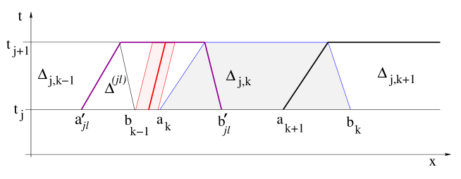
Figure 5: Implementing a post-processing algorithm, each strip $[t_{j},t_{j+1}]\times{\mathbb{R}}$ is covered with trapezoids $\Delta_{jk}$ where the oscillation remains small (as far as possible), and trapezoids $\Delta^{(j\ell)}$ containing a large traced shock.

The next result provides an a posteriori estimate on the ${\bf L}^{1}$ error in the approximate solution. Here the estimate refers to the outcome of a post-processing algorithm, depending on the choice of the parameters $\rho,K$ in the definition of flagged points at (7.1). We remark that any choice of such parameters leads to some error bound. However, the sharpness of the estimate heavily depends on a suitable choice of these parameter values.

Theorem 5.1

Consider a system of conservation laws satisfying the basic assumptions (A1)-(A2). Then there exist constants $C^{\prime},C^{\prime\prime}$ such that the following holds.

Let $u:[0,T]\times{\mathbb{R}}\mapsto{\mathbb{R}}^{n}$ be an approximate solution to the Cauchy problem (1.1)-(1.2), satisfying the conditions (AL) and (P_ε), together with (5.1). Let $\kappa_{j}$, $\kappa^{\prime}$ be the oscillation bounds in (3.5) and (5.4), for a covering with trapezoids $\Delta_{jk}$, $\Delta^{(j\ell)}$ produced by a post-processing algorithm. Then the difference between $u(T,\cdot)$ and the exact solution is bounded by

$$\begin{array}[]{l}\displaystyle\bigl{\|}u(T,\cdot)-S_{T}\bar{u}\bigr{\|}_{{\bf L}^{1}({\mathbb{R}})}~{}\leq~{}C^{\prime}\left(T+\sum_{j=0}^{\nu-1}\kappa_{j}\right)\varepsilon^{1/3}+C^{\prime\prime}\left(\varepsilon^{1/3}\kappa^{\prime}+\varepsilon^{2/3}\right)\cdot\sum_{j=0}^{\nu-1}N^{\prime}(j)\,.\end{array}$$ (5.9)

Proof. 1. Calling $L_{0}$ be the Lipschitz constant of the semigroup at (1.7), we have

$$\|u(T,\cdot)-S_{T}\bar{u}\|_{{\bf L}^{1}}~{}\leq~{}L_{0}\cdot\sum_{j=0}^{\nu-1}\Big{\|}u(t_{j+1},\cdot)-S_{h}u(t_{j},\cdot)\Big{\|}_{{\bf L}^{1}}\,.$$ (5.10)

For each $j$, in order to estimate the difference $u(t_{j+1},\cdot)-S_{h}u(t_{j},\cdot)$, we consider a covering of the strip $[t_{j},t_{j+1}]\times{\mathbb{R}}$ by trapezoids $\Delta^{(j\ell)}$, $\ell=1,\ldots N^{\prime}(j)$ as in (5.6), and $\Delta_{jk}$, $k=1,\ldots,N(j)$, as in (5.7). 2. Recalling (4.3), we denote by $\{t_{j+1}\}\times[a_{j\ell},b_{j\ell}]$ the upper boundaries of the trapezoids $\Delta^{(j\ell)}$. These are the trapezoids which contain one large traced shock. Moreover, we call $\{t_{j+1}\}\times[\widehat{c}_{jk},\widehat{d}_{jk}]$ the upper boundaries of the remaining trapezoids $\Delta_{jk}$. According to (5.7), this means

$$[\widehat{c}_{jk}\,,\,\widehat{d}_{jk}]~{}=~{}\Big{[}c_{jk}+h\lambda^{+}+\varepsilon^{2/3}~{},~{}d_{jk}+h\lambda^{-}-\varepsilon^{2/3}\Big{]}.$$

3. The same argument used at (3.17) now yields an error bound on the set

$$V_{j}~{}\doteq~{}\bigcup_{k=1}^{N(j)}~{}[\widehat{c}_{jk}\,,\,\widehat{d}_{jk}].$$

Indeed, recalling the uniform bound (5.1) on the total variation, one obtains

$$\int_{V_{j}}\Big{|}u(t_{j+1},x)-\left(S_{h}u(t_{j},\cdot)\right)(x)\Big{|}\,dx~{}\leq~{}C_{3}\left(\kappa_{j}\,h+\varepsilon^{2/3}+h\varepsilon^{1/3}\right)\cdot\delta_{0}\,.$$ (5.11)

On the other hand, for each $\ell\in\{1,\ldots,N^{\prime}(j)\}$, applying the estimate (4.11) on the interval $[a_{j\ell},b_{j\ell}]$ we obtain the error bound

$$\int_{a_{j\ell}}^{b_{j\ell}}\bigl{|}u(h,x)-(S_{h}\bar{u})(x)\bigr{|}\,dx~{}\leq~{}C_{5}\cdot h\,\left({\varepsilon\over\rho}+\kappa^{\prime}+{\rho\kappa^{\prime}+\delta\over h}\right)+C_{5}\,\left(\rho\kappa^{\prime}+h\kappa^{\prime}+\delta\right).$$ (5.12)

4. Recalling our choices

$$\rho~{}=~{}h~{}=~{}\varepsilon^{1/3},\qquad\delta~{}=~{}\varepsilon^{2/3},\qquad\nu h~{}=~{}\nu\varepsilon^{1/3}~{}=~{}T,$$

summing the terms in (5.11) over all $j\in\{0,\ldots,\nu-1\}$, and summing the terms in (5.12) over all $j$ and all $\ell\in\{1,\ldots,N^{\prime}(j)\}$, we obtain (5.9). MM     

Remark 5.1

It is interesting to speculate about the rate at which the error bound on the right hand side of (5.9) will approach zero as $\varepsilon\to 0$. We begin by assuming that the exact solution we are trying to compute is piecewise Lipschitz, with a finite number of centered rarefaction waves, and finitely many non-interacting shocks.

As is Remark 3.1, the first term on the right hand side of (5.9) is expected to approach zero as $\varepsilon^{1/3}|\log\varepsilon|$. Concerning the second term, we can fix a constant $C_{0}$ and choose $\kappa^{\prime}=C_{0}\varepsilon^{1/3}$. If the exact solution contains $N^{\prime}$ shocks, we expect that, for all $\varepsilon>0$ sufficiently small, each of these shocks will be traced, satisfying the inequality (5.2). The second term on the right hand side of (5.9) will thus have the form

$$C^{\prime\prime}\left(\varepsilon^{1/3}C_{0}\varepsilon^{1/3}+\varepsilon^{2/3}\right)\cdot\nu N^{\prime}~{}=~{}{\cal O}(1)\cdot\varepsilon^{1/3}.$$

In this case, (5.9) would yield

$$\bigl{\|}u(T,\cdot)-S_{T}\bar{u}\bigr{\|}_{{\bf L}^{1}({\mathbb{R}})}~{}=~{}{\cal O}(1)\cdot\varepsilon^{1/3}|\log\varepsilon|.$$ (5.13)

More generally, let us now assume that some of the shocks in the solution interact with each other. Let $\tau\in[0,T]$ be one of the (finitely many) interaction times. During a time interval $[\tau^{-},\tau^{+}]$ around $\tau$, of size $\tau^{+}-\tau^{-}={\cal O}(1)\cdot\rho$, we shall not be able to trace the interacting shocks. As a consequence, for $[t_{j},t_{j+1}]\cap[\tau^{-},\tau^{+}]\not=\emptyset$, the oscillation on one of the trapezoids $\Delta_{jk}$ in (5.7) (the one which contains a non-traced shock) will be large. This will force $\kappa_{j}$ to be large. However, we expect that the total length of all intervals $[t_{j},t_{j+1}]$, where some large shock cannot be traced, will have size

$${\cal O}(1)\cdot\rho\cdot\hbox{[total number of shock interactions]}~{}=~{}{\cal O}(1)\cdot\varepsilon^{1/3}.$$

In conclusion, the presence of finitely many shock interactions will contribute an additional error term ${\cal O}(1)\cdot\varepsilon^{1/3}$ to the right hand side of (5.9). This will not change its overall order of magnitude.

One could also argue that, if the solution contains a finite number of compression waves, from which new shocks are formed, these (non-traced) waves would contribute an error term of the same nature as a centered rarefaction wave. Therefore, a bound of the order (5.13) would still be obtained.

Once again, we emphasize that the bounds (5.13) represent only a heuristic expectation. For a numerically computed solution, they needs to be confirmed by a post-processing algorithm, computing a bound on the oscillations $\kappa_{j}$ in (3.5).

6 Properties of approximation schemes

In this section we analyze various approximation methods, and check that they verify the assumptions (AL) and (P_ε). Our a posteriori error estimates can thus be applied to all of them.

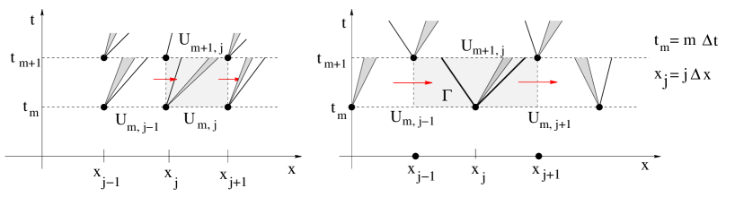
Figure 6: Left: the upwind Godunov scheme is obtained by solving the Riemann problems at each node $P_{mj}=(t_{m},x_{j})$, then by replacing each solution by its average on each of the intervals $[x_{j},x_{j+1}]$. By the conservation equation, these averages can be explicitly computed by (6.2). Right: a similar construction leads to the Lax-Friedrichs scheme (6.12).

6.1 The Godunov scheme.

To simplify our discussion, we assume that all characteristic speeds (i.e., all eigenvalues of the Jacobian matrices $Df(u)$) lie in the interior of the interval $[0,1]$. In this case, the Godunov scheme reduces to an upwind scheme. Given a mesh size $\varepsilon>0$, consider the grid points

$$P_{mj}=(t_{m},x_{j})~{}=~{}(\varepsilon m,\varepsilon j).$$

As shown in Fig. 6, left, we consider approximate solutions $u=u(t,x)$ with the following properties:

• At each time $t=t_{m}$, the function $u(t_{m},\cdot)$ is piecewise constant, namely

  $$u(t_{m},x)~{}=~{}U_{mj}\qquad\hbox{for}\quad x_{j}<x<x_{j+1}\,,$$

• For $t\in[t_{m},t_{m+1}[\,$, the function $u(t,\cdot)$ yields the exact solution to (1.1) with initial data $u(t_{m},\cdot)$. This is obtained by solving the Riemann problems at each node $x_{j}$.

• At time $t_{m+1}$, we take the average of $u(t_{m+1}-\,,\cdot)$ on each interval $[x_{j},x_{j+1}]$. Namely

  $$u(t_{m+1},x)~{}=~{}U_{m+1,j}~{}\doteq~{}{1\over\varepsilon}\int_{x_{j}}^{x_{j+1}}u(t_{m+1},y)\,dy\qquad\hbox{for}\quad x_{j}<x<x_{j+1}\,.$$ (6.1)

  Since we are assuming that all wave speeds are contained in the interval $[0,1]$, using the conservation equations these average values $U_{m+1,j}$ can be computed by

  $$U_{m+1,\,j}~{}=~{}U_{m,j}+\Big{(}f(U_{m,j-1})-f(U_{m,j})\Big{)}.$$ (6.2)

We check that an approximate solution $u$ produced by the Godunov scheme with mesh size $\varepsilon>0$ satisfies the Lipschitz condition (AL). Indeed, for every $0\leq\tau<\tau^{\prime}\leq T$ with $\tau,\tau^{\prime}\in\varepsilon{\mathbb{N}}$,

$$\begin{array}[]{l}\bigl{\|}u(\tau^{\prime},\cdot)-u(\tau,\cdot)\bigr{\|}_{{\bf L}^{1}({\mathbb{R}})}~{}\leq\displaystyle\sum_{\tau<t_{m}\leq\tau^{\prime}}\sum_{j}\int_{x_{j-1}}^{x_{j}}\bigl{|}u(t_{m+1},x)-u(t_{m},x)\bigr{|}\,dx\\[11.38109pt] \displaystyle\qquad=~{}\sum_{\tau<t_{m}\leq\tau^{\prime}}\sum_{j}\varepsilon\Big{|}f(U_{m,j-1})-f(U_{m,j})\Big{|}~{}\leq~{}\varepsilon\,\sum_{\tau<t_{m}\leq\tau^{\prime}}\hbox{Tot.Var.}\Big{\{}f(u(t_{m},\cdot))\Big{\}}\\[11.38109pt] \displaystyle\qquad\leq~{}(\tau^{\prime}-\tau)\cdot\hbox{Lip}(f)\cdot\sup_{t\in[\tau,\tau^{\prime}]}\hbox{\rm Tot.Var.}\bigl{\{}u(t,\cdot)\bigr{\}}.\end{array}$$ (6.3)

To prove that the property (P_ε) also holds, we shall use

Lemma 6.1

Let $w:[0,\varepsilon]\mapsto{\mathbb{R}}$ be any function with bounded variation, and assume $\varphi\in{\cal C}^{1}$. Consider the average value

$$\overline{w}~{}\doteq~{}{1\over\varepsilon}\int_{0}^{\varepsilon}w(y)\,dy.$$

Then

$$\left|\int_{0}^{\varepsilon}[w(x)-\overline{w}]\,\varphi(x)\,dx\right|~{}\leq~{}\hbox{\rm Tot.Var.}\bigl{\{}w\,;~{}]0,\varepsilon[\,\bigr{\}}\cdot\varepsilon^{2}\|\varphi_{x}\|_{{\bf L}^{\infty}}\,.$$ (6.4)

Proof. Call $\overline{\varphi}$ the average value of $\varphi$ over $[0,\varepsilon]$. Then

$$\begin{array}[]{l}\displaystyle\left|\int_{0}^{\varepsilon}[w(x)-\overline{w}]\,\varphi(x)\,dx\right|~{}=~{}\left|\int_{0}^{\varepsilon}[w(x)-\overline{w}]\,(\varphi(x)-\overline{\varphi})\,dx\right|\\[11.38109pt] \qquad\leq\displaystyle\int_{0}^{\varepsilon}\|w(\cdot)-\overline{w}\|_{{\bf L}^{\infty}}\cdot\,\|\varphi(\cdot)-\overline{\varphi}\|_{{\bf L}^{\infty}}\,dx~{}\leq~{}\varepsilon\cdot\hbox{\rm Tot.Var.}\bigl{\{}w\,;~{}]0,\varepsilon[\,\bigr{\}}\cdot\varepsilon\|\varphi_{x}\|_{{\bf L}^{\infty}}\,.\end{array}$$ (6.5)

MM     

Next, fix $\varepsilon>0$ and consider any test function $\varphi\in{\cal C}^{1}_{c}({\mathbb{R}}^{2})$. Since the Godunov approximations coincide with exact solutions on each of the half-open intervals $[t_{m},t_{m+1}[\,$, we have

$$\begin{array}[]{l}\displaystyle\left|\int u(\tau,x)\varphi(\tau,x)\,dx-\int u(\tau^{\prime},x)\varphi(\tau^{\prime},x)\,dx+\int_{\tau}^{\tau^{\prime}}\int\bigl{\{}u\varphi_{t}+f(u)\varphi_{x}\bigr{\}}~{}dxdt\right|\\[11.38109pt] \qquad\displaystyle=~{}\left|\sum_{\tau<t_{m}\leq\tau^{\prime}}\int[u(t_{m},x)-u(t_{m}-,x)]\varphi(t_{m},x)\,dx\right|.\end{array}$$ (6.6)

Using Lemma 6.1 we obtain

$$\begin{array}[]{l}\displaystyle\sum_{\tau<t_{m}\leq\tau^{\prime}}\left|\int[u(t_{m},x)-u(t_{m}-,x)]\,\varphi(t_{m},x)\,dx\right|\\[11.38109pt] \displaystyle\qquad\leq~{}\sum_{\tau<t_{m}\leq\tau^{\prime}}\sum_{j}\varepsilon^{2}\,\hbox{\rm Tot.Var.}\Big{\{}u(t_{m},\cdot)\,;~{}]j\varepsilon,(j+1)\varepsilon[\,\Big{\}}\cdot\|\varphi_{x}(t_{m},\cdot)\|_{{\bf L}^{\infty}}\\[14.22636pt] \qquad\displaystyle=~{}\varepsilon\,(\tau^{\prime}-\tau)\|\varphi_{x}\|_{{\bf L}^{\infty}}\cdot\sup_{t\in[\tau,\tau^{\prime}]}\hbox{\rm Tot.Var.}\bigl{\{}u(t,\cdot)\bigr{\}}.\end{array}$$ (6.7)

This yields (1.11). In order to prove (P_ε), given a convex entropy with entropy flux $q$, it remains to check that (1.12) is satisfied as well. Let $\varphi\geq 0$ be a test function in $\mathcal{C}^{1}_{c}({\mathbb{R}}^{2})$. Integration by parts yields

$$\begin{array}[]{l}\displaystyle\int\eta(u(\tau,x))\varphi(\tau,x)\,dx-\int\eta(u(\tau^{\prime},x))\varphi(\tau^{\prime},x)\,dx+\int_{\tau}^{\tau^{\prime}}\int{\eta(u)\varphi_{t}+q(u)\varphi_{x}}~{}dt~{}dx\\[8.53581pt] \displaystyle=~{}-\int_{\tau}^{\tau^{\prime}}\int\{\eta(u)_{t}+q(u)_{x}\}\varphi~{}dx~{}dt+\sum_{\tau<t_{m}\leq\tau^{\prime}}\int(\eta(u(t_{m}-,x))-\eta(u(t_{m},x)))\varphi(t_{m},x)dx.\end{array}$$ (6.8)

By construction, the approximation $u$ is an entropy weak solution of the hyperbolic system of conservation law in every strip $[t_{m-1},t_{m}[\times{\mathbb{R}}$, therefore the first term on the right hand side of (6.8) is non negative.

By the convexity of $\eta$, we can apply Jensen’s inequality and obtain

$$\eta(u(t_{m},x))~{}=~{}\eta\Big{(}{1\over\varepsilon}\int_{x_{j}}^{x_{j+1}}u(t_{m}-,y)\,dy\Big{)}~{}\leq~{}{1\over\varepsilon}\int_{x_{j}}^{x_{j+1}}\eta(u(t_{m}-,y))\,dy\,,$$ (6.9)

for $x_{j}<x<x_{j+1}$. In turn, this yields

$$\begin{array}[]{l}\displaystyle\sum_{\tau<t_{m}\leq\tau^{\prime}}\int_{{\mathbb{R}}}(\eta(u(t_{m}-,x))-\eta(u(t_{m},x)))\varphi(t_{m},x)dx\\[8.53581pt] \displaystyle~{}=~{}\sum_{\tau<t_{m}\leq\tau^{\prime}}\sum_{j}\int_{x_{j}}^{x_{j+1}}(\eta(u(t_{m}-,x))-\eta(u(t_{m},x)))\varphi(t_{m},x)\,dx\\[8.53581pt] \displaystyle~{}\geq~{}\sum_{\tau<t_{m}\leq\tau^{\prime}}\sum_{j}\int_{x_{j}}^{x_{j+1}}\Big{(}\eta(u(t_{m}-,x))-\int_{x_{j}}^{x_{j+1}}\eta(u(t_{m}-,y))\,dy\Big{)}\varphi(t_{m},x)\,dx\\[8.53581pt] \displaystyle~{}\geq~{}-\,\hbox{Lip}(\eta)\,\varepsilon\cdot(\tau^{\prime}-\tau)\|\varphi_{x}\|_{{\bf L}^{\infty}}\cdot\sup_{t\in[\tau,\tau^{\prime}]}\hbox{\rm Tot.Var.}\bigl{\{}u(t,\cdot)\bigr{\}}.\end{array}$$ (6.10)

6.2 The Lax-Friedrichs scheme.

Consider step sizes $\Delta t,\Delta x>0$ so that all characteristic speeds satisfy the CFL condition

$$|\lambda_{i}|~{}<~{}{\Delta x\over\Delta t}\,.$$ (6.11)

As shown in Fig. 6, right, we then construct a staggered grid with nodes at the points

$$P_{mj}~{}=~{}(m\,\Delta t,\,j\,\Delta x),\qquad\qquad m+j~{}\hbox{even}.$$

The Lax-Friedrichs approximations are defined inductively as follows. Given a piecewise constant function $u(t_{m},\cdot)$, with jumps at the points $P_{mj}$ with $m+j$ even, for $t\in[t_{m},t_{m+1}[$ we let $u(t,\cdot)$ be the exact solution of the system of conservation laws (1.1) with the given data at $t=t_{m}$. We then define $u(t_{m+1},\cdot)$ to be the piecewise constant function obtained by taking the average of $u(t_{m+1}-,\cdot)$ over every interval $[x_{j-1},x_{j+1}]$ with $m+j$ even. By the conservation equations, if all characteristic speeds satisfy $|\lambda_{i}|<\Delta x/\Delta t$, these average values

$$U_{m+1,j}~{}=~{}{1\over 2\Delta x}\int_{x_{j-1}}^{x_{j+1}}u(t_{m+1}-,\,x)\,dx\,,\qquad\qquad m+j~{}\hbox{even},$$

are inductively computed by the Lax-Friedrichs scheme

$$U_{m+1,j}~{}=~{}{1\over 2}(U_{m,j+1}+U_{m,j-1})-{\Delta t\over 2\Delta x}\bigl{[}f(U_{m,j+1})-f(U_{m,j-1})\bigr{]}.$$ (6.12)

Setting $\varepsilon=\Delta t$, both the approximate Lipschitz condition (AL) and the property (P_ε) can be proved in the same way as for the Godunov scheme. We thus omit details.

6.3 Backward Euler approximations.

We now discretize time but keep space continuous. We assume that all characteristic speeds are strictly positive. Calling $\varepsilon=\Delta t$ the time step, and setting $U_{m}(x)=u(m\varepsilon,x)$, the backward Euler approximations are defined in terms of implicit equations

$$u(t+\varepsilon,x)~{}=~{}u(t,x)-\varepsilon f(u(t+\varepsilon,x))_{x}\,.$$

Equivalently:

$$U_{m+1}(x)~{}=~{}U_{m}(x)-\varepsilon\,f(U_{m+1}(x))_{x}\,.$$ (6.13)

At the present time, the convergence of these approximations for general $n\times n$ hyperbolic systems is not known. Complete results are available in the scalar case [20], which can be handled by the general theory of nonlinear contractive semigroups [21]. Let $U_{m}(\cdot)$ be a sequence of solutions to (6.13) with $m=0,1,\ldots$ and define the approximate solution $u$ by setting

$$u(t,x)=U_{m}(x)\qquad\hbox{ for }\quad m\varepsilon\leq t<(m+1)\varepsilon.$$

Then (AL) follows by

$$\begin{array}[]{rl}\bigl{\|}u(\tau,\cdot)-u(\tau^{\prime},\cdot)\bigr{\|}_{{\bf L}^{1}({\mathbb{R}})}&\leq~{}\displaystyle\sum_{\tau<t_{m}\leq\tau^{\prime}}\bigl{\|}u(t_{m},\cdot)-u(t_{m-1},\cdot)\bigr{\|}_{{\bf L}^{1}({\mathbb{R}})}\\[11.38109pt] &=~{}\displaystyle\varepsilon\sum_{\tau<t_{m}\leq\tau^{\prime}}\int\bigl{|}f(u(t_{m},x))_{x}\bigr{|}\,dx\\[11.38109pt] &\leq~{}\hbox{Lip}(f)\,(\tau^{\prime}-\tau)\cdot\Big{(}\sup_{t\in[\tau,\tau^{\prime}]}\hbox{Tot.Var.}\{u(t,\cdot)\}\Big{)}.\end{array}$$

Next, we check that (P_ε) holds. As before, fix $0\leq\tau<\tau^{\prime}\leq T$ with $\tau,\tau^{\prime}\in\varepsilon{\mathbb{N}}$. Given a test function $\varphi\in\mathcal{C}^{1}_{c}({\mathbb{R}}^{2})$, we compute

$$\begin{array}[]{l}\displaystyle\left|\int u(\tau,x)\varphi(\tau,x)\,dx-\int u(\tau^{\prime},x)\varphi(\tau^{\prime},x)\,dx+\int_{\tau}^{\tau^{\prime}}\int\bigl{\{}u\varphi_{t}+f(u)\varphi_{x}\bigr{\}}\,dx\,dt\right|\\[11.38109pt] \qquad=\displaystyle~{}\left|-\int_{\tau}^{\tau^{\prime}}\int f(u)_{x}\varphi\,dx\,dt+\int_{\mathbb{R}}{\sum_{\tau<t_{m}\leq\tau^{\prime}}\Big{(}u(t_{m-1},x)-u(t_{m},x)\Big{)}\varphi(t_{m-1},x)}~{}dx\right|\\[11.38109pt] \qquad\displaystyle\leq~{}\bigg{|}-\int\left(\sum_{\tau<t_{m}\leq\tau^{\prime}}\frac{u(t_{m-1},x)-u(t_{m},x)}{\varepsilon}\int_{t_{m-1}}^{t_{m}}\varphi(t,x)dt\right)dx\\[11.38109pt] \qquad\qquad\qquad\displaystyle+\int\sum_{\tau<t_{m}\leq\tau^{\prime}}{\Big{(}u(t_{m-1},x)-u(t_{m},x)\Big{)}\varphi(t_{m-1},x)}\,dx\bigg{|}\\[11.38109pt] \qquad\displaystyle\leq~{}\int\sum_{\tau<t_{m}\leq\tau^{\prime}}\big{|}u(t_{m-1},x)-u(t_{m},x)\big{|}\left|\varphi(t_{m-1},x)-\frac{1}{\varepsilon}\int_{t_{m-1}}^{t_{m}}\varphi(t,x)dt\right|dx\\[11.38109pt] \qquad\displaystyle\leq~{}\varepsilon\,(\tau^{\prime}-\tau)\,\|\varphi\|_{W^{1,\infty}}\hbox{Lip}(f)\cdot\Big{(}\sup_{t\in[\tau,\tau^{\prime}]}\hbox{Tot.Var.}\{u(t,\cdot)\}\Big{)}.\end{array}$$

Finally, let $\eta$ be a convex entropy with entropy flux $q$. If $\varphi\geq 0$ is a test function in $\mathcal{C}^{1}_{c}({\mathbb{R}}^{2})$, we have

$$\begin{array}[]{l}\displaystyle\int\eta(u(\tau,x))\varphi(\tau,x)\,dx-\int\eta(u(\tau^{\prime},x))\varphi(\tau^{\prime},x)\,dx+\int_{\tau}^{\tau^{\prime}}\int\{\eta(u)\varphi_{t}+q(u)\varphi_{x}\}~{}dx~{}dt\\[11.38109pt] ~{}=~{}\displaystyle-\int_{\tau}^{\tau^{\prime}}\int q(u)_{x}\varphi~{}dt~{}dx+\int{\sum_{\tau<t_{m}\leq\tau^{\prime}}\Big{(}\eta(u(t_{m-1},x))-\eta(u(t_{m},x))\Big{)}\varphi(t_{m-1},x)}~{}dx\\[11.38109pt] ~{}=~{}\displaystyle-\sum_{\tau<t_{m}\leq\tau^{\prime}}\int\Big{(}D\eta(u(t_{m},x))\cdot\frac{u(t_{m-1},x)-u(t_{m},x)}{\varepsilon}\int_{t_{m-1}}^{t_{m}}\varphi(t,x)dt\Big{)}dx\\[11.38109pt] \qquad\qquad\qquad\qquad\displaystyle+\int{\sum_{\tau<t_{m}\leq\tau^{\prime}}\Big{(}\eta(u(t_{m-1},x))-\eta(u(t_{m},x))\Big{)}\varphi(t_{m-1},x)}\,dx\\[11.38109pt] \displaystyle\geq~{}\sum_{\tau<t_{m}\leq\tau^{\prime}}\int\Big{(}\eta(u(t_{m-1},x))-\eta(u(t_{m},x)\Big{)}\Big{(}\varphi(t_{m-1},x)-\frac{1}{\varepsilon}\int_{t_{m-1}}^{t_{m}}\varphi(t,x)dt\Big{)}dx\\[11.38109pt] \displaystyle\geq~{}-\varepsilon\,(\tau^{\prime}-\tau)\,\|\varphi\|_{W^{1,\infty}}\hbox{Lip}(\eta)\hbox{Lip}(f)\cdot\Big{(}\sup_{t\in[\tau,\tau^{\prime}]}\hbox{Tot.Var.}\{u(t,\cdot)\}\Big{)}.\end{array}$$

Notice that the convexity of $\eta$ was here used in the inequality

$$D\eta(u(a,x))\cdot\Big{(}u(a,x)-u(b,x)\Big{)}~{}\geq~{}\eta(u(a,x))-\eta(u(b,x).$$ (6.14)

6.4 The smoothing method.

Next, we consider an approximate solution to (1.1)-(1.2) obtained by periodic mollifications, taking the convolution with a smoothing kernel $K\in{\cal C}^{\infty}_{c}({\mathbb{R}})$. As usual, we assume

$$\left\{\begin{array}[]{rl}K(x)&>~{}0\quad\hbox{for}~{}|x|<1,\\[5.69054pt] K(x)&=~{}0\quad\hbox{for}~{}|x|\geq 1,\end{array}\right.\qquad K(x)=K(-x),\qquad\int K(x)\,dx~{}=~{}1,$$ (6.15)

and set $K_{\delta}(x)\doteq\delta^{-1}K(\delta^{-1}x)$. We fix a time step $\varepsilon>0$ and define an $\varepsilon$-approximate solution $u$ by setting

$$t_{m}~{}=~{}m\,\varepsilon,\qquad u(t_{m},\cdot)~{}=~{}K_{\delta}*u(t_{m}-,\cdot),$$

and letting $u$ be a classical solution to (1.1) on each half-open interval $[t_{m},t_{m+1}[\,$.

As in the scalar case (see [26]), the method is well-defined provided that the ratio $\varepsilon/\delta$ is suitably small. To see this, in connection with the quasilinear system

$$u_{t}+A(u)u_{x}~{}=~{}0,\qquad\qquad A(u)\,=\,Df(u),$$ (6.16)

we choose bases $\{r_{1}(u),\ldots,r_{n}(u)\}$ and $\{l_{1}(u),\ldots,l_{n}(u)\}$ of right and left eigenvectors of $A(u)$, normalized so that

$$|r_{i}(u)|\,=\,0,\qquad\qquad l_{i}(u)\cdot r_{i}(u)~{}=~{}\left\{\begin{array}[]{rl}1\quad\hbox{if}~{}i=j,\cr 0\quad\hbox{if}~{}i\not=j.\end{array}\right.$$ (6.17)

We denote by $u_{x}^{i}\,=\,l_{i}\cdot u_{x}$ the $i$-th component of the gradient vector $u_{x}$ w.r.t. this basis. From (6.17) and (6.16) it follows

$$u_{x}~{}=~{}\sum_{i=1}^{n}u_{x}^{i}r_{i}(u)\qquad\qquad u_{t}~{}=~{}-\sum_{i=1}^{n}\lambda_{i}(u)u^{i}_{x}r_{i}(u).$$

Differentiating the first equation w.r.t. $t$ and the second one w.r.t. $x$, then equating the results, one obtains a semilinear system of evolution equations for the scalar components $u_{x}^{i}$, having the form

$$(u_{x}^{i})_{t}+\lambda_{i}(u_{x}^{i})_{x}~{}=~{}\sum_{j,k=1}^{n}g^{i}_{jk}(u)u_{x}^{j}u_{x}^{k}.$$ (6.18)

See for example Section 1.6 in [9] for details. Assume that

$$\bigl{|}g^{i}_{jk}(u)\bigr{|}~{}<~{}M_{g}$$

for all $i,j,k$, and all $u$ in the domain were the solution is defined. Let $t\mapsto Z(t)$ be the solution to the ODE

$${d\over dt}Z(t)~{}=~{}n^{2}M_{g}\,Z^{2}(t),\qquad\qquad Z(0)\,=\,Z_{0}\,.$$ (6.19)

Assume that, at time $t=0$, there holds

$$\bigl{|}u^{i}_{x}(0,x)\bigr{|}~{}\leq~{}Z_{0}\qquad\hbox{for all}~{}x\in{\mathbb{R}},~{}~{}i=1,\ldots,n.$$ (6.20)

A comparison argument now yields

$$\bigl{|}u^{i}_{x}(t,x)\bigr{|}~{}\leq~{}Z(t)\qquad\hbox{for all}~{}x\in{\mathbb{R}},~{}t\in[0,T_{0}[\,,$$

where

$$T_{0}~{}=~{}{1\over n^{2}M_{g}\,Z_{0}}$$

is the time where the solution to (6.19) blows up.
It remains to give an upper bound for the gradient components after each mollification. This is achieved observing that

$$\begin{array}[]{l}\displaystyle\|u_{x}^{i}(t_{m},\cdot)\|_{{\bf L}^{\infty}}~{}\leq~{}\|u_{x}(t_{m},\cdot)\|_{{\bf L}^{\infty}}\cdot\sup_{u}\,|l_{i}(u)|\\[8.53581pt] \qquad~{}\leq~{}\displaystyle{\hbox{\rm Tot.Var.}\{u(t_{m}-,\cdot)\}\over\delta}\,\|K\|_{{\bf L}^{\infty}}\cdot\sup_{u}\,|l_{i}(u)|.\end{array}$$

Therefore, if we choose

$$0<\varepsilon<{\delta\over n^{2}\,M_{g}\,\|K\|_{{\bf L}^{\infty}}}\,\Big{(}\sup_{m}\hbox{\rm Tot.Var.}\{u(t_{m}-,\cdot)\}\Big{)}^{-1}\Big{(}\sup_{i}\sup_{u}|l_{i}(u)|\Big{)}^{-1},$$

all the components $u^{i}_{x}$ remain bounded on each strip $[t_{m},t_{m+1}[\times{\mathbb{R}}$, and the approximate solution is well-defined.

We now check that the assumption (AL) holds:

$$\begin{array}[]{lr}\bigl{\|}u(\tau^{\prime},\cdot)-u(\tau,\cdot)\bigr{\|}_{{\bf L}^{1}({\mathbb{R}})}\\[11.38109pt] \displaystyle~{}\leq~{}\sum_{\tau<t_{m}\leq\tau^{\prime}}\int\bigl{|}~{}K_{\delta}*u(t_{m}-,x)-u(t_{m}-,x)|\,dx+\sum_{\tau<t_{m}\leq\tau^{\prime}}\int\bigl{|}u(t_{m}-,x)-u(t_{m-1},x)|\,dx\\[11.38109pt] \displaystyle~{}\leq~{}\delta\Big{(}{\tau^{\prime}-\tau\over\varepsilon}\Big{)}\cdot\sup_{t\in[\tau,\tau^{\prime}]}\hbox{\rm Tot.Var.}\bigl{\{}u(t,\cdot)\bigr{\}}+L\,(\tau^{\prime}-\tau)\cdot\sup_{t\in[\tau,\tau^{\prime}]}\hbox{\rm Tot.Var.}\bigl{\{}u(t,\cdot)\bigr{\}}\\[11.38109pt] \displaystyle~{}=~{}C\,(\tau^{\prime}-\tau)\cdot\sup_{t\in[\tau,\tau^{\prime}]}\hbox{\rm Tot.Var.}\bigl{\{}u(t,\cdot)\bigr{\}}.\end{array}$$

Here we are using the estimate

$$\begin{array}[]{lr}\displaystyle\int\bigl{|}~{}K_{\delta}*u(t_{m}-,x)-u(t_{m}-,x)|\,dx\\[11.38109pt] ~{}\displaystyle\leq~{}\int_{-\delta}^{\delta}K_{\delta}(y)\sup_{|y|\leq\varepsilon}\Big{(}\int|u(t_{m}-,x)-u(t_{m}-,x-y)|\,dx\Big{)}\,dy\\[11.38109pt] ~{}\leq~{}\delta~{}\hbox{\rm Tot.Var.}\{u(t_{m}-,\cdot)\}.\end{array}$$ (6.21)

To prove (P_ε) we shall need the following result.

Lemma 6.2

Let $w:{\mathbb{R}}\mapsto{\mathbb{R}}$ be any function with bounded variation, and assume $\varphi\in{\cal C}^{1}$. Let $K\in{\cal C}^{\infty}_{c}$ be a smoothing kernel as in (6.15) and define

$$\widetilde{w}~{}\doteq~{}K_{\delta}\ast w.$$

Then

$$\left|\int[\widetilde{w}(x)-w(x)]\,\varphi(x)\,dx\right|~{}=~{}{\cal O}(1)\cdot\delta^{2}\cdot\|\varphi\|_{W^{1,\infty}}\cdot\hbox{\rm Tot.Var.}\{w\}\,.$$ (6.22)

Proof. We rewrite the left hand side of (6.22) in a more suitable way:

$$\begin{array}[]{l}\displaystyle\left|\int[\widetilde{w}(x)-w(x)]\,\varphi(x)\,dx\right|\\[8.53581pt] ~{}=~{}\displaystyle\left|\int\!\!\!\int K_{\delta}(x-y)[w(y)-w(x)]\,\varphi(x)\,dy\,dx\right|\\[8.53581pt] ~{}=~{}\displaystyle\left|\int\!\!\!\int K_{\delta}(x-y)[\varphi(y)-\varphi(x)]\,w(x)\,dy\,dx\right|\\[8.53581pt] ~{}=~{}\displaystyle\left|\int\left(\int_{-\infty}^{x}\int K_{\delta}(x-y)[\varphi(y)-\varphi(x)]\,dydz\right)w^{\prime}(x)\,dx\right|.\end{array}$$ (6.23)

Next we prove the estimate

$$\left|\int_{-\infty}^{x}\int K_{\delta}(z-y)[\varphi(y)-\varphi(z)]\,dydz\right|~{}=~{}{\cal O}(1)\cdot\delta^{2}\cdot\|\varphi\|_{W^{1,\infty}}\,.$$ (6.24)

The integral in (6.24) can be split in

$$\begin{array}[]{l}\displaystyle\int_{-\infty}^{x}\int K_{\delta}(z-y)[\varphi(y)-\varphi(z)]\,dydz\\[8.53581pt] ~{}=~{}\displaystyle\int_{-\infty}^{x-\delta}\int_{z-\delta}^{z+\delta}K_{\delta}(z-y)[\varphi(y)-\varphi(z)]\,dydz+\int_{x-\delta}^{x}\int_{z-\delta}^{z+2x-\delta}K_{\delta}(z-y)[\varphi(y)-\varphi(z)]\,dydz\\[8.53581pt] \quad\quad\quad\quad~{}+~{}\displaystyle\int_{x-\delta}^{x}\int_{z+2x-\delta}^{z+\delta}K_{\delta}(z-y)[\varphi(y)-\varphi(z)]\,dydz\end{array}$$ (6.25)

and by introducing the change of coordinates $y={q-t\over 2}$ and $z={q+t\over 2}$ it follows that

$$\begin{array}[]{l}\displaystyle\int_{-\infty}^{x-\delta}\int_{z-\delta}^{z+\delta}K_{\delta}(z-y)[\varphi(y)-\varphi(z)]\,dydz+\int_{x-\delta}^{x}\int_{z-\delta}^{z+2x-\delta}K_{\delta}(z-y)[\varphi(y)-\varphi(z)]\,dydz\\[8.53581pt] \quad\quad~{}=~{}\displaystyle\int_{-\infty}^{2x-\delta}\int_{-\delta}^{\delta}K_{\delta}(t)\Big{[}\varphi\Big{(}{q-t\over 2}\Big{)}-\varphi({q+t\over 2})\Big{]}dt\,dq\\[8.53581pt] \quad\quad~{}=~{}\displaystyle 0.\end{array}$$

Therefore the only contribution is given by the last integral in (6.25). Calling $\Sigma$ be its domain of integration, we find

$$\begin{array}[]{rl}\displaystyle\left|\int\!\!\!\int_{\Sigma}K_{\delta}(z-y)[\varphi(y)-\varphi(z)]\,dydz\right|&\displaystyle\leq~{}\hbox{meas}(\Sigma)\cdot\|K_{\delta}\|_{{\bf L}^{\infty}}\cdot\sup_{(x,y)\in\Sigma}|\varphi(y)-\varphi(z)|\\[11.38109pt] &\displaystyle=~{}\delta^{2}\cdot C\delta^{-1}\cdot 2\delta\,\|\varphi\|_{W^{1,\infty}}\,,\end{array}$$ (6.26)

Together with (6.23), this yields (6.22). MM     

Now consider any test function $\varphi\in\mathcal{C}^{1}_{c}({\mathbb{R}}^{2})$. Using the above lemma, we obtain

$$\begin{array}[]{lr}\displaystyle\left|\int u(\tau,x)\varphi(\tau,x)\,dx-\int u(\tau^{\prime},x)\varphi(\tau^{\prime},x)\,dx+\int_{\tau}^{\tau^{\prime}}\int\bigl{\{}u\varphi_{t}+f(u)\varphi_{x}\bigr{\}}\,dx\,dt\right|\\[11.38109pt] ~{}\displaystyle=~{}\left|\int\sum_{\tau<t_{j}\leq\tau^{\prime}}\bigl{(}u(t_{j},x)-u(t_{j}-,x)\bigr{)}\,\varphi(t_{j},x)dx\right|\\[11.38109pt] ~{}\displaystyle\leq~{}C_{1}\,\delta^{2}\Big{(}{\tau^{\prime}-\tau\over\varepsilon}\Big{)}\|\varphi\|_{W^{1,\infty}}\cdot\Big{(}\sup_{t\in[\tau,\tau^{\prime}]}\hbox{Tot.Var.}\{u(t,\cdot)\}\Big{)}\\[11.38109pt] ~{}\displaystyle=~{}C_{2}\,\varepsilon\,(\tau^{\prime}-\tau)\|\varphi\|_{W^{1,\infty}}\cdot\Big{(}\sup_{t\in[\tau,\tau^{\prime}]}\hbox{Tot.Var.}\{u(t,\cdot)\}\Big{)}.\end{array}$$

Finally, let $\eta$ be a convex entropy with entropy flux $q$. For any non-negative test function $\varphi\in{\cal C}^{1}_{c}({\mathbb{R}}^{2})$ one has

$$\begin{array}[]{lr}\displaystyle\int\eta(u(\tau,x))\varphi(\tau,x)\,dx-\int\eta(u(\tau^{\prime},x))\varphi(\tau^{\prime},x)\,dx+\int_{\tau}^{\tau^{\prime}}\int\bigl{\{}\eta(u)\varphi_{t}+q(u)\varphi_{x}\bigr{\}}\,dx\,dt\\[11.38109pt] ~{}\displaystyle=~{}-\int\sum_{\tau<t_{m}\leq\tau^{\prime}}\Big{(}\eta(u(t_{m},x))-\eta(u(t_{m}-,x))\Big{)}\,\varphi(t_{m},x)dx\\[11.38109pt] ~{}\displaystyle\geq~{}-\int\sum_{\tau<t_{m}\leq\tau^{\prime}}~{}D\eta(u(t_{m},x))\big{(}u(t_{m},x)-u(t_{m}-,x)\big{)}\,\varphi(t_{m},x)dx\\[11.38109pt] ~{}\displaystyle\geq~{}-C_{1}\,\delta^{2}\,\Big{(}{\tau^{\prime}-\tau\over\varepsilon}\Big{)}\|\varphi\|_{W^{1,\infty}}\,\hbox{Lip}(\eta)\cdot\Big{(}\sup_{t\in[\tau,\tau^{\prime}]}\hbox{Tot.Var.}\{u(t,\cdot)\}\Big{)}\\[11.38109pt] ~{}\displaystyle=~{}-C_{2}\,\varepsilon\,({\tau^{\prime}-\tau})\|\varphi\|_{W^{1,\infty}}\,\hbox{Lip}(\eta)\cdot\Big{(}\sup_{t\in[\tau,\tau^{\prime}]}\hbox{Tot.Var.}\{u(t,\cdot)\}\Big{)}\,,\end{array}$$

where the first inequality follows from the strict convexity of $\eta$, by (6.14).

7 Numerical implementation

In this last section we discuss details of the post-processing algorithm, and present a numerical simulation.

STEP 1 of the algorithm, computing the total variation of the numerical solution $u(t,\cdot)$, is entirely straightforward.

STEP 2, identifying the location of the large shocks, requires more attention. Given a pair of constants $K>0$ and $\sigma>\!>\varepsilon>0$, we first identify regions where the total variation of $u$ is large. For this purpose, we introduce

Definition 7.1

For a given function $u:[0,T]\times{\mathbb{R}}\mapsto{\mathbb{R}}^{n}$, the points $(t,x)$ such that

$$\min\Big{\{}\hbox{\rm Tot.Var.}\bigl{\{}u(t,\cdot)\,;~{}[x-\sigma,x+\varepsilon]\bigr{\}}~{},~{}~{}\hbox{\rm Tot.Var.}\bigl{\{}u(t,\cdot)\,;~{}[x-\varepsilon,\,x+\sigma]\bigr{\}}\Big{\}}~{}>~{}K\sigma$$ (7.1)

will be called flagged points.

Notice that, by definition, the oscillation of $u(t_{j},\cdot)$ on a small interval to the left or to the right of a flagged point must be large. Roughly speaking, the following result shows that, outside flagged points, solutions are approximately Lipschitz continuous with constant $2K$.

Lemma 7.1

Assume that all points $(t,x)$ with $x\in[a,b]$ are not flagged. Then

$$|u(t,a)-u(t,b)|~{}\leq~{}\left(1+{b-a\over\sigma+\varepsilon}\right)2\sigma K\,.\qquad$$ (7.2)

Proof. 1. By assumption, we can split the interval as $[a,b]=I^{+}\cup I^{-}$, where $I^{+},I^{-}$ are two disjoint sets with the following property. Setting

$$J_{x}~{}=~{}\left\{\begin{array}[]{rl}[x-\varepsilon,x+\sigma]&\hbox{if}\quad x\in I^{+},\\[8.53581pt] [x-\sigma,x+\varepsilon]&\hbox{if}\quad x\in I^{-},\end{array}\right.$$

one has

$$\hbox{\rm Tot.Var.}\{u(t,\cdot);~{}J_{x}\}~{}\leq~{}\sigma K\qquad\hbox{for all}~{}x\in[a,b].$$

2. We claim that every subinterval $[c,d]\subseteq[a,b]$ with length $d-c\leq\sigma+\varepsilon$ can be covered by two of the intervals $J_{x}$. Indeed, three cases can arise:

CASE 1: $c+\varepsilon\in I^{+}$. Then $[c,d]\subseteq J_{c+\varepsilon}\,$.

CASE 2: $d-\varepsilon\in I^{-}$. Then $[c,d]\subseteq J_{d-\varepsilon}\,$.

CASE 3: $c+\varepsilon\in I^{-}$ and $d-\varepsilon\in I^{+}$. Then we can find to points $c+\varepsilon\leq x<y\leq d-\varepsilon$, such that

$$y-x<\varepsilon,\qquad x\in I^{-},~{}y\in I^{+}.$$

In this case, $[c,d]\subseteq J_{x}\cup J_{y}$, proving our claim. 3. To complete the proof, we cover $[a,b]$ with finitely many intervals $[c_{i},d_{i}]$, $i=1,\ldots,N$, such that

$$N~{}\leq~{}1+{b-a\over\sigma+\varepsilon}\,,\qquad\quad d_{i}-c_{i}~{}\leq~{}\sigma+\varepsilon\qquad\hbox{for all}~{}i=1,\ldots,N,$$

By the previous construction, for every $i$ we have

$$\hbox{\rm Tot.Var.}\bigl{\{}u(t,\cdot)\,;~{}[c_{i},d_{i}]\bigr{\}}~{}\leq~{}2K\sigma.$$

Therefore, the total variation of $u(t,\cdot)$ over $[a,b]$ is bounded by $2N\sigma K$. This yields (7.2). MM     

Having defined the set ${\cal F}\subseteq[0,T]\times{\mathbb{R}}$ of all flagged points, for each $t_{j}=j\varepsilon\in[0,T]$, $j=0,1,\ldots,\nu$, we denote by

$${\cal F}_{j}~{}\doteq~{}\bigl{\{}x\in{\mathbb{R}}\,;~{}~{}(t_{j},x)\in{\cal F}\bigr{\}}$$

the set of flagged points at time $t_{j}$.

For every time $t_{j}$, we identify intervals $[a,b]$ such that $b-a\leq\delta\doteq\varepsilon^{2/3}$ and moreover

$$a\in{\cal F}_{j}\,,\qquad b\in{\cal F}_{j}\,,\qquad{\cal F}_{j}\cap[a-\rho,a[~{}=~{}{\cal F}_{j}\,\cap\,]b,b+\rho]~{}=~{}\emptyset.$$

In other words, the points $(t_{j},a)$ and $(t_{j},b)$ are flagged, but points to the left of $a$ and to the right of $b$ are not flagged.

Each such interval $[a,b]$ locates a possible isolated shock at time $t_{j}$. To check if this shock can be traced over the entire interval $[t_{j},t_{j+1}]$, we check if there exists an interval $[c,d]$ with the same properties at time $t=t_{j+1}$, with

$$[c,d]~{}\subset~{}[a+\lambda^{-}h~{},~{}b+\lambda^{+}h].$$

In the positive case, we approximate the shock location as

$$\gamma(t)~{}=~{}x_{0}+\lambda(t-t_{j})$$

choosing $x_{0},\lambda$ so that

$$\gamma(t_{j})~{}=~{}{a+b\over 2}\,,\qquad\qquad\gamma(t_{j+1})~{}=~{}{c+d\over 2}.$$

We then consider the polygonal regions $\Gamma$, $\Delta_{l}$, $\Delta^{\prime}_{r}$ defined as in (5.3). If the two inequalities (5.4)-(5.5) are both satisfied, we say that the parallelogram

$$\Gamma~{}=~{}\Big{\{}(t,x)\,;~{}t\in[t_{j},t_{j+1}]\,,~{}~{}x_{0}-\delta+(t-t_{j})\lambda\,\leq\,x\,\leq\,x_{0}+\delta+\lambda^{-}(t-t_{j})\Big{\}},$$

traces the shock. The trapezoid

$$\Delta^{\prime}~{}=~{}\Big{\{}(t,x)\,;~{}t\in[t_{j},t_{j+1}]\,,~{}~{}a^{\prime}+\lambda^{+}(t-t_{j})\,\leq\,x\,\leq\,b^{\prime}+\lambda^{-}(t-t_{j})\Big{\}},$$

$$a^{\prime}~{}\doteq~{}x_{0}-\rho-\delta-(\lambda^{+}-\lambda^{-})h,\qquad b^{\prime}~{}\doteq~{}x_{0}+\rho+\delta+(\lambda^{+}-\lambda^{-})h,$$

is then inserted within the list of trapezoids $\Delta^{(j\ell)}$ in (5.6), containing a traced shock. On the other hand, if one of the inequalities (5.4)-(5.5) fails, the shock is not traced. STEP 3 of the algorithm provides a covering of each domain

$$\Big{(}[t_{j},t_{j+1}]\times{\mathbb{R}}\Big{)}\setminus\bigcup_{\ell=1}^{N^{\prime}(j)}\Delta^{(j\ell)},\qquad\quad j=0,1,\ldots,\nu-1,$$

with finitely many trapezoids $\Delta_{jk}$ as in (5.7). This step is straightforward. The algorithm terminates by computing the constants $\kappa_{j}$ in (5.8), which provide an upper bound on the oscillation of $u$ on each $\Delta_{jk}$.

Example. We consider a model of isentropic gas dynamics in Lagrangian coordinates. Using a shifted system of coordinates, this can be written as

$$\left\{\begin{array}[]{rl}v_{t}-u_{x}+v_{x}&=~{}0,\\[8.53581pt] \displaystyle u_{t}+\left({1\over 2v^{2}}\right)_{x}+u_{x}&=0.\end{array}\right.$$ (7.3)

Here $u$ is the velocity of the gas, while $v$ denotes the specific volume. By the choice of coordinates, the characteristic speeds are

$$\lambda^{\pm}~{}=~{}1\pm v^{-3/2}.$$

In particular, when $v\geq 1$, one has $\lambda(v)\in[\lambda^{-},\lambda^{+}]\doteq[0,2]$. We consider the Cauchy problem with piecewise constant initial data

$$v(0,x)~{}=~{}\left\{\begin{array}[]{cl}2&\hbox{if}~{}~{}x<0,\cr 3&\hbox{if}~{}~{}0<x<{1/2},\cr 1&\hbox{if}~{}~{}x>{1/2},\end{array}\right.\qquad\qquad u(0,x)~{}=~{}0.$$ (7.4)

The exact solution is shown in Fig. 7.

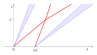
Figure 7: A sketch of the exact solution to (7.3)-(7.4), containing two centered rarefaction waves and two shocks, interacting at time $t^{*}$.

We compute an approximate solution using the Godunov upwind scheme with mesh sizes

$$\Delta x\,=\,\varepsilon\,=\,0.0005,\qquad\qquad\Delta t\,=\,{\varepsilon\over 2}\,=\,0.00025\,.$$

The profiles of the two components of the solution, at the terminal time $T=1.5$, are shown in Fig. 8.

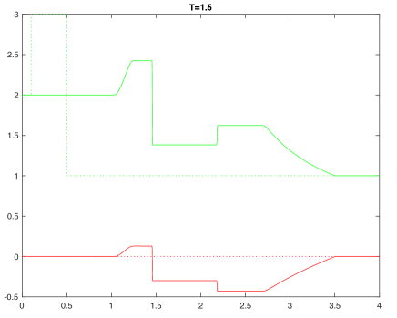
Figure 8: The components of the solution at the terminal time $T=1.5$, computed by the Godunov scheme. Above: the specific volume $v(T,\cdot)$. Below: the velocity $u(T,\cdot)$.

To illustrate how the post-processing algorithm works, in Fig. 9, left, we plot the set of flagged points. These are computed according to Definition 7.1, choosing $\sigma=0.0063$ and $K=25$. In Fig. 9, right, we identifying the shocks that can be traced on each time interval $[t_{j},t_{j+1}]$. Here $\kappa^{\prime}=0.1$, $\sigma_{min}=0.4$. Notice that, according to our previous construction, each trapezoid $\Delta^{(j\ell)}$ around a traced shock will have the form

$$\Delta^{(j\ell)}~{}=~{}\Big{\{}(t,x)\,;~{}~{}t\in[t_{j},\,t_{j+1}],~{}~{}x_{j\ell}-\delta-\rho-2h+2(t-t_{j})~{}\leq~{}x~{}\leq~{}x_{j\ell}+\delta+\rho+2h\Big{\}}.$$

Indeed, this is obtained from (4.3)-(4.4), with

$$a^{\prime}\,=~{}\,x_{j\ell}-\delta-\rho-2h,\qquad b^{\prime}\,=\,x_{j\ell}+\delta+\rho+2h,\qquad\lambda^{-}=0,\qquad\lambda^{+}=2.$$

 

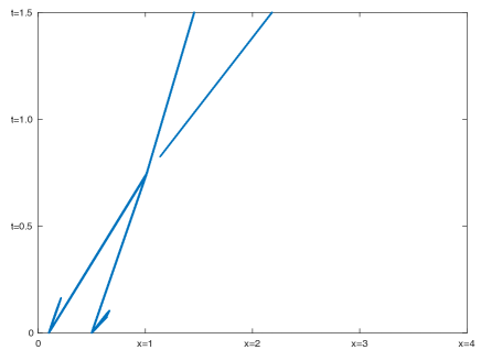
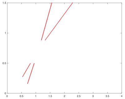
Figure 9: Left: the points flagged by the post-processing algorithm. Right: the portions of the two shocks that are actually traced.

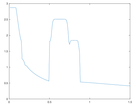
Figure 10: An approximate computation of the function $\kappa(t)$ at (7.5), determining the error rate.

Finally, in Fig. 10 we plot an approximate graph of the function

$$\kappa(t)~{}=~{}\kappa_{j}~{}\doteq~{}\max_{1\leq k\leq N(j)}\hbox{\rm Osc.}\{u\,;~{}\Delta_{jk}\}\qquad\hbox{if}~{}~{}t\in[t_{j},t_{j+1}\,[\,.$$ (7.5)

One can think of $\kappa(t)$ as the maximum oscillation of the numerical solution $u(t,\cdot)$ on domains of diameter ${\cal O}(1)\cdot\varepsilon^{1/3}$, outside the large traced shocks. In view of (5.9), this function $\kappa(\cdot)$ determines the rate at which the distance $\|u(t,\cdot)-S_{t}\bar{u}\|_{{\bf L}^{1}}$ between the approximate and the exact solution increases in time. Notice that $\kappa(t)$ is large for $t\approx 0$, when the main contribution to the error comes from the two centered rarefactions. As time increases, the rarefactions decay, and the value of $\kappa(t)$ decays as well. As $t$ approaches the interaction time $t^{*}$, the two shocks cannot be individually traced. As a consequence, the value of $\kappa(t)$ suddenly becomes very large. Finally, when the shocks move away from each other and can be traced once again, we see that $\kappa(t)$ regains its small values.

Acknowledgments. This research was partially supported by NSF with grant DMS-2006884, “Singularities and error bounds for hyperbolic equations”.

References

[1] F. Ancona and A. Marson,
Sharp convergence rate of the Glimm scheme for general nonlinear hyperbolic systems.
Comm. Math. Phys.302 (2011), 581–630.
[2] P. Baiti, A. Bressan, and H. K. Jenssen,
BV instability of the Godunov scheme,
Comm. Pure Appl. Math.59 (2006), 1604–1638.
[3] S. Bianchini, BV solutions of the semidiscrete upwind
scheme. Arch. Rational Mech. Anal. 167 (2003), 1–81.
[4] S. Bianchini, Hyperbolic limit of the
Jin-Xin relaxation
model. Comm. Pure Appl. Math. 59 (2006), 688–753.
[5] S. Bianchini and A. Bressan, Vanishing viscosity
solutions of nonlinear hyperbolic systems. Annals Math.161
(2005), 223–342.
[6] S. Bianchini and
S. Modena,
Convergence rate of the Glimm scheme.
Bull. Inst. Math. Acad. Sinica11 (2016), 235–300.
[7] A. Bressan, The unique limit of the Glimm scheme, Arch. Rational
Mech. Anal.130 (1995), 205–230.
[8] A. Bressan, Hyperbolic systems of conservation laws.
The one-dimensional Cauchy problem. Oxford University Press, Oxford, 2000.
[9] A. Bressan, Hyperbolic conservation laws: an
illustrated tutorial.
In “Modelling and Optimisation of Flows on Networks”.
Edited by
L. Ambrosio, A. Bressan, D. Helbing, A. Klar, and E. Zuazua.
Springer Lecture Notes in Mathematics2062 (2012), pp.157–245.
[10] A. Bressan and R. M. Colombo,
The semigroup generated by conservation laws,
Arch. Rational Mech. Anal.113 (1995), 1–75.
[11] A. Bressan, G. Crasta, and B. Piccoli,
Well posedness of the Cauchy problem for systems
of conservation laws, Amer. Math. Soc. Memoir694 (2000).
[12] A. Bressan and P. Goatin,
Oleinik type estimates and uniqueness for
conservation laws, J. Differential Equations156 (1999), 26–49.
[13] A. Bressan, F. Huang, Y. Wang, and T. Yang,
On the convergence rate of
vanishing viscosity approximations for nonlinear hyperbolic systems,
SIAM J. Math. Analysis44 (2012), 3537–3563.
[14] A. Bressan and H. K. Jenssen,
On the convergence of Godunov scheme for nonlinear hyperbolic
systems,
Chinese Ann. Math.B - 21 (2000), 1–16.
[15] A. Bressan and P. LeFloch,
Uniqueness of weak solutions to systems of conservation laws,
Arch. Rational Mech. Anal.140 (1997), 301–317.
[16] A. Bressan and M. Lewicka, A uniqueness condition for hyperbolic systems of conservation laws, Discr. Cont. Dyn. Syst.6 (2000), 673–682.
[17] A. Bressan, T. P. Liu, and T. Yang, stability
estimates for conservation laws. Arch. Rational Mech. Anal. 149 (1999), 1–22.
[18] A. Bressan and A. Marson, Error bounds for a deterministic version of the Glimm scheme,
Arch. Rational Mech. Anal.142 (1998), 155–176.
[19] A. Bressan and T. Yang, On the rate of convergence of vanishing viscosity
approximations, Comm. Pure Appl. Math.57 (2004), 1075–1109.
[20]
M. G. Crandall,
The semigroup approach to first order quasilinear equations
in several space variables.
Israel J. Math.12 (1972), 108–132.
[21]
M. G. Crandall and T. M. Liggett, Generation of semigroups of nonlinear transformations on general Banach spaces. Amer. J. Math.93 (1971), 265–298.
[22] C. Dafermos, Hyperbolic Conservation Laws in Continuum Physics,
Fourth edition. Springer-Verlag, Berlin, 2016.
[23] X. Ding, G. Q. Chen, and P. Luo, Convergence of the
fractional step Lax-Friedrichs scheme and Godunov scheme for the isentropic
system of gas dynamics. Comm. Math. Phys. 121
(1989), 63–84.
[24] J. Glimm, Solutions in the large for nonlinear hyperbolic
systems of equations. Comm. Pure Appl. Math. 18 (1965),
697–715.
[25] S. K. Godunov, A difference method for numerical
calculation of discontinuous solutions of the equations of hydrodynamics.
(Russian) Mat. Sb. (N.S.) 47 (89) (1959), 271–306.
[26] H. Holden and N. Risebro, Front Tracking for Hyperbolic Conservation Laws.
Springer-Verlag, Berlin, 2002.
[27]
S. Jin and Z. Xin, The relaxation schemes for systems of conservation laws in arbitrary space dimensions.
Comm. Pure Appl. Math.48 (1995), 235–277.
[28] P. Lax, Weak solutions of nonlinear hyperbolic
equations and their numerical computation. Comm. Pure Appl. Math. 7 (1954), 159–193.
[29] P. Lax, Hyperbolic systems of conservation
laws II. Comm. Pure Appl. Math. 10 (1957), 537–566.
[30] R. J. LeVeque, Numerical methods for conservation
laws. Birkhäuser-Verlag, Basel, 1990.
[31] T. P. Liu, The deterministic version of the Glimm scheme,
Comm. Math. Phys.57 (1975), 135-148.