Learning to be safe, in finite time

Abstract

This paper aims to put forward the concept that learning to take safe actions in unknown environments, even with probability one guarantees, can be achieved without the need for an unbounded number of exploratory trials, provided that one is willing to relax its optimality requirements mildly. We focus on the canonical multi-armed bandit problem and seek to study the exploration-preservation trade-off intrinsic within safe learning. More precisely, by defining a handicap metric that counts the number of unsafe actions, we provide an algorithm for discarding unsafe machines (or actions), with probability one, that achieves constant handicap. Our algorithm is rooted in the classical sequential probability ratio test, redefined here for continuing tasks. Under standard assumptions on sufficient exploration, our rule provably detects all unsafe machines in an (expected) finite number of rounds. The analysis also unveils a trade-off between the number of rounds needed to secure the environment and the probability of discarding safe machines. Our decision rule can wrap around any other algorithm to optimize a specific auxiliary goal since it provides a safe environment to search for (approximately) optimal policies. Simulations corroborate our theoretical findings and further illustrate the aforementioned trade-offs.

I Introduction

Learning to take safe actions in unknown environments is a general goal that spans across multiple disciplines. Within control theory safety is intrinsic to robust analysis and design [1], where controllers, with stability and performance guarantees, are designed for uncertain systems. It is also at the core of statistical decision theory [2], where the inference and the decision-making processes are intertwined towards the common goal of making accurate decisions based on limited information. Though, historically, these two disciplines have been deemed as seemingly disconnected, such separation is rapidly vanishing.

Motivated by the success of machine learning in achieving super human performance, e.g., in vision [3, 4], speech [5, 6], and video games [7, 8], there has been recent interest in developing learning-enabled technology that can implement highly complex actions for safety-critical autonomous systems, such as self-driving cars, robots, etc. However, without proper safety guarantees such systems will rarely be deployed. There is therefore the need to develop analysis tools and algorithms that can provide such guarantees during, and after, training.

A common approach to solve this problem is to search for actions, policies, or controllers that optimize a cost or reward subject to safety requirements imposed as constraints. Examples include, adding safe constraints for reinforcement learning algorithms [9, 10, 11, 12, 13], (robust) stability constraints to learning algorithms [14, 15, 16], and solving constrained multi-armed bandits [17, 18]. When such constraints are being included during training, algorithms that converge to optimal policies, guarantee safety asymptotically. However, such an approach fails to provide guarantees while learning.

In this paper, we suggest an alternative approach. Instead of focusing on finding optimal actions subject to, a priori unknown, safety constrains, we argue that one should tackle the problem of learning safe actions separately and more efficiently. To illustrate this point, we study the problem of finding safe actions within the canonical setting of the multi-armed bandit (MAB) problem. This setting lacks state transitions and is thus an abridged version of learning in dynamical environments. In the MAB setting, one is given a set of $N$ machines/actions with expected reward $\mu_{n}\in[0,1]$ for $n\in\{1,\dots,N\}$. By letting safe actions to be those who choose machines with reward larger than some nominal $\mu$, we define a handicap metric —akin to regret— that counts the number of times unsafe actions are chosen. Leveraging classical results on sequential hypothesis tests [19], we provide an algorithm for detecting unsafe machines. Unlike the regret minimization counterpart of this problem, which requires an unbounded (with logarithmic growth) number of trials of sub-optimal actions to identify the machine with highest reward [20], our algorithm discards all unsafe machines with only a finite number of trials of unsafe actions. By characterizing such number, we guarantee that the total handicap remains bounded by a constant.

More precisely, we use a modified version of Wald’s sequential probability ratio test (SPRT) [19] for each machine, with the null ($H_{0}$) and alternative ($H_{1}$) hypothesis being that the machine is safe and unsafe, respectively. Intentionally different than the SPRT, which aims to decide either $H_{0}$ or $H_{1}$ and then stop, our goal is to discard unsafe machines only by deciding on $H_{1}$. This allows our algorithm to identify all unsafe machines with probability one within a finite expected number of trials. Our analysis also unveils an exploration-preservation trade-off between the false-positive ratio (safe machines discarded) and the total handicap experienced (number of trials on unsafe machines). Notably, our decision rule can further wrap around any other algorithm to optimize a specific auxiliary goal since it provides a safe environment to search for (approximately) optimal policies.

The rest of the paper is organized as follows. We introduce our problem setup in Section II. For didactic purposes, we first look at the case where we aim to find machines with $\mu=1$ in Section III, construct a sequential test that extends this case for one machine in Section IV, and generalize the solution in Section V. Numerical illustrations are provided in Section VI and we conclude in Section VII.

II Problem statement

Consider the setup of a multi-armed bandit problem, in which at each time instant $t=1,2,\ldots$ we have the choice to operate one out of $N$ machines. If machine $n\in\{1,2,\ldots,N\}$ is operated at time $t$, it returns a binary value $X_{n,t}$ which is modelled as a Bernoulli random variable with parameter $\mu_{n}$. This return reveals whether the action led to a safe result in which case $X_{n,t}=1$, or an unsafe one if $X_{n,t}=0$. A machine is said to be safe if its operation leads to a safe result. In this sense we consider two cases, one in which we only accept flawless machines, i.e., those with $\mu_{n}=1$, and a relaxed condition in which a machine is defined to be safe if $\mu_{n}\geq\mu$, with $\mu\in(0,1)$ being a prescribed safety requirement (possibly $\mu\simeq 1$).

Let $I_{t}\in\{1,2,\ldots,N\}$ denote the index of the machine selected at time $t$, and $X_{t}\doteq X_{I_{t},t}$ the corresponding return. Our goal is to design a selection policy and a decision rule that uses data $X_{t},\ t=1,2,\ldots$ to remove all unsafe machines, while guaranteeing that a prescribed proportion of the safe machines are kept. If only flawless machines are accepted then the solution is straightforward: the algorithm should remove machines as soon as they return their first $X_{t}=0$. We will analyse this case first in Section III.

For the relaxed condition, we will develop a one-sided Sequential Probability Ratio Test (SPRT) that removes unsafe machines with $\mu_{n}\leq\mu$ almost surely. In order to guarantee that unsafe machines are removed in finite time, and provide an explicit bound on the expected number of trials needed, we need to sacrifice a proportion of the safe machines. For this purpose we prescribe a slack parameter $\epsilon$ and a probability $\alpha$, and show that a proportion $1-\alpha$ of those safe machines with $\mu_{n}\geq\mu+\epsilon$ are kept as $t\to\infty$. We will develop this modified version of the SPRT in Section IV for the case of $N=1$, extending it in Section V to the multi-armed bandit setup.

Along the way, we will introduce three figures of merits that are instrumental to goal of learning to be safe. One is the handicap, that complements the idea of regret for operating unsafe machines, and counts the number of unsafe actions chosen so far. Closely related to the notion of handicap is the testing time, that counts the number of times a machine is tried for safety, and is related to the detection time of unsafe machines. The third one is the safety ratio, which counts the proportion of safe machines that are kept at time $t$.

III Safe learning with flawless machines

Consider the multi armed bandit setup described above with $N$ machines, $M$ of them unsafe or malfunctioning. In order to simplify notation and without loss of generality, we assume that the first $M$ machines are unsafe so that $\mu_{n}<1$ for $n=1,\ldots,M$, and $\mu_{n}=1$ for $n=M+1,\ldots,N$.

We are assured that $X_{n,t}=1~{}\forall t$ if the machine is safe, thus we can discard those machines that return $X_{n,t}=0$. This is the strategy in Algorithm 1, which selects actions at random over the set $\mathcal{S}_{t}$ of machines that remain at time $t$.

Initialize $\mathcal{S}_{1}=\left\{1,\ldots,N\right\}$

for $t=1,2,\ldots,$ do

       Pick an arm $I_{t}\sim$ Unif($\mathcal{S}_{t}$)

       Observe return $X_{t}=X_{I_{t},t}$

       if $X_{t}=0$ then

            $\mathcal{S}_{t}\leftarrow\mathcal{S}_{t-1}\setminus\{I_{t}\}$

       end if

      else

            $\mathcal{S}_{t}\leftarrow\mathcal{S}_{t-1}\;$

       end if

      

end for

Algorithm 1 Safety Inspector

The following definitions are introduced for the purpose of analysing the Safety Inspector Algorithm 1 and its relaxed version in Section V. First, even if we recognize that detecting unsafe machines requires unsafe actions to be taken, we want to measure if our algorithms pick those unsafe machines efficiently. For this purpose we present the notion of handicap, defined as the number of times an unsafe machine is selected, i.e.,

$$\operatorname{Handicap}_{t}=t-\sum_{\tau=1}^{t}\mathds{1}\{\mu_{I_{\tau}}\geq\mu\}$$ (1)

where $\mu=1$ in this section, and $\mathds{1}(\cdot)$ represents the indicator function which returns one or zero when its argument is true or false, respectively.

Remark.

We use the word handicap in the sense of a measure of “a disadvantage that makes achievement unusually difficult,” as its definition suggests [21]. An algorithm with unbounded $\operatorname{Handicap}_{t}$ takes unsafe actions infinitely often and is prone to malfunctioning. This marks a stark contrast with the notion of regret, typically studied in Bandit settings [22], where unbounded regret is unavoidable [20].

Notice that if machine $n$ is selected at time $\tau$, then $\mu_{I_{\tau}}=\mu_{n}$. Thus, the indicator function will return $1$ at time $\tau$ only when a flawless machine is selected. Furthermore, even if $\mu_{n}$ is deterministic, $\operatorname{Handicap}_{t}$ is still a random variable, with randomness coming from the selection $I_{t}$. Even if $I_{t}$ is selected in round-robin instead of uniformly as in Algorithm 1, the set $\mathcal{S}_{t}$ is conditioned on previous instances of $X_{t}$, which are uncertain. In light of this, it is noticeable that an algorithm with low handicap is one which selects unsafe machines infrequently. As a second figure of merit we define the safety ratio $\rho_{t}$ as the proportion of safe machines that are kept after $t$ time slots, i.e.,

$$\rho_{t}=\frac{\sum_{n\in\mathcal{S}_{t}}\mathds{1}(\mu_{n}\geq\mu+\epsilon)}{N-M}$$ (2)

with $\epsilon=0$ for Algorithm 1. Together with the notions of handicap and safety ratio, we are interested in analysing the time that elapses until an unsafe machine is removed. For this purpose it is instrumental to define the number of times that machine $n$ has been tested for safety after $t$ iterations of Algorithm 1, that is

$$T_{n}(t)=\sum_{\tau=1}^{t}\mathds{1}(I_{\tau}=n).$$ (3)

Next, we present a lemma that links the definitions of $\operatorname{Handicap}_{t}$ with $T_{n}(t)$, and will be useful to bound the expected handicap for Algorithm 1 and that in Section V.

Lemma 1.

$\mathbb{E}[{\emph{Handicap}_{t}}]=\sum_{n=1}^{M}\mathbb{E}[T_{n}(t)]$

Proof.

$$\mathbb{E}[\operatorname{Handicap}_{t}]=\sum_{\tau=1}^{t}\mathbb{E}\left[\mathds{1}\{\mu_{I_{\tau}}<\mu\}\right]$$

$$=\sum_{\tau=1}^{t}\sum_{n=1}^{N}P(I_{\tau}=n)\mathds{1}\{\mu_{I_{\tau}}<\mu\}=\sum_{\tau=1}^{t}\sum_{n=1}^{M}P(I_{\tau}=n)$$

$$=\sum_{n=1}^{M}\sum_{\tau=1}^{t}\mathbb{E}\left[\mathds{1}\{I_{\tau}=n\}\right]=\sum_{n=1}^{M}\mathbb{E}[T_{n}(t)]$$

∎

Using the result in Lemma 1 we can bound the expected handicap of Algorithm 1 by bounding $\mathbb{E}[T_{n}(t)]$. This is the result of the next Theorem.

Theorem 1.

The handicap and safety ratio of Algorithm 1 satisfy

$$\mathbb{E}[\emph{Handicap}_{t}] \leq\sum_{n=1}^{M}\frac{1}{(1-\mu_{n})}$$ (4)

$$\mathbb{E}[\rho_{t}] =1,$$ (5)

and the testing time of unsafe machines is bounded by

$$\mathbb{E}[T_{n}(t)] \leq\frac{1}{(1-\mu_{n})}$$ (6)

Proof.

The result for the safety ratio is straightforward since the probability of removing a machine with $\mu_{n}=1$ is zero. The bound for the handicap follows from Lemma 1, together with the result for the testing time, which is proved next

$$\mathbb{E}[T_{n}(t)] =\sum_{\tau=1}^{t}\text{P}(T_{n}(t)=\tau)\tau=\sum_{\tau=1}^{t}\mu_{n}^{\tau-1}(1-\mu_{n})\;\tau$$ (7)

$$\leq\sum_{\tau=1}^{\infty}\mu_{n}^{\tau-1}(1-\mu_{n})\;\tau=\frac{1}{1-\mu_{n}}$$ (8)

∎

Remark.

The right hand side of (7) in Theorem 1 bounds the expected number of times that an unsafe machine is tested before removing it. This highlights one of the main ideas introduced in this paper: if we only want to detect unsafe machines instead of estimating the exact value of $\mu_{n}$, then we can do it in finite time. As a consequence, the measure of handicap defined in (1) remains bounded by a constant. Even if we deem this result as conceptually relevant, it presents the drawback that the bounds for the expected handicap and testing times are given in terms of $\mu_{n}$ which are unknown. In order to provide an explicit bound in terms of the design parameters of the algorithm it is convenient to relax the condition that defines a safe machine, allowing for machines with $\mu_{n}\geq\mu$ lowering the prescribed safety threshold to $\mu<1$. By doing so, we will retain the ability of rejecting all unsafe machines almost surely, while explicitly bounding the handicap. With this goal in mind, we present our modified SPRT in the next section.

IV Sequential probability ratio test

Consider in this section the case of a single machine with unknown mean $\mu_{n}$. We face the problem of deciding whether the machine is unsafe, i.e., $\mu_{n}\leq\mu<1$. For this purpose, we set the following Hypothesis test

$$\begin{cases}H_{0}\mathrel{\mathop{\mathchar 58\relax}}&\mu_{n}\geq\mu+\epsilon\\ H_{1}\mathrel{\mathop{\mathchar 58\relax}}&\mu_{n}\leq\mu\end{cases}$$ (9)

where $\epsilon\leq 1-\mu$ is a slack parameter. The goal of this section is to devise a sequential test, which uses data $X_{t}$ for $t=1,2,\ldots$ to detect if the machine is unsafe. We look for a test that detects such a machine almost surely, and that guarantees that a machine with $\mu_{n}\geq\mu+\epsilon$ is kept with probability $1-\alpha$ as $t$ grows unbounded. The three values $\mu$, $\epsilon$ and $\alpha$ are design parameters. An overly conservative choice, $\epsilon\simeq 0$ $\alpha\simeq 0$ pays the price of a longer detection time, as shown in Lemma 4 later in this section. The construction of the following test and the analysis of cylinder sets are based on Wald’s celebrated SPRT [19].

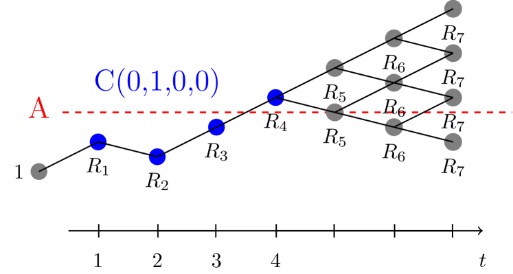
Figure 1: Schematic of the decision rule for the one-sided SPRT (11). Sequences $\{x_{t}\}_{t=1}^{\infty}$ belonging to the cylinder set $C(0,1,0,0)$ coincide in the first $t=4$ entries $(x_{1},x_{2},x_{3},x_{4})=(0,1,0,1)$, which determine the likelihood ratios $(L_{1},L_{2},L_{3},L_{4})$ represented by blue points. Since they cross the decision threshold $A$ at $T=4$, the null hypothesis is rejected and the machine is declared unsafe. The decision is made at $T=4$, and therefore the multiple possible trajectories of $L_{t}$ afterwards are inconsequential and can be disregarded.

Let $f_{\mu}(x)$ and $f_{\mu+\epsilon}(x)$ denote the probability mass functions corresponding to the Bernoulli distributions of parameters $\mu$ and $\mu+\epsilon$, respectively. For $t\in\mathbb{N}$ consider a sampled trajectory $(x_{1},\ldots,x_{t})$ and define the likelihood ratio:

$$L_{t}=\frac{f_{\mu}\left(x_{1},x_{2},\ldots,x_{t}\right)}{f_{\mu+\epsilon}\left(x_{1},x_{2},\ldots,x_{t}\right)}$$ (10)

At each time we calculate $L_{t}$ and accept $H_{1}$ if

$$L_{t}\geq A$$ (11)

where the threshold $A$ is a design parameter that will be specified later. This is, if $L_{t}\geq A$ we declare that the machine is unsafe and stop the test. Otherwise we take an additional observation pulling the arm one more time to then check the condition (11) again after updating $t\to t+1$. Assuming i.i.d. samples, (11) can be transformed into a condition on the number of zeros $k_{t}$ in the trajectory $(x_{1},x_{2},\ldots,x_{t})$. Indeed, taking the logarithm of (10), (11) transforms into $k_{t}\lambda_{0}-(t-k_{t})\lambda_{1}\geq\log A$, with $\lambda_{0}\mathrel{\mathop{\mathchar 58\relax}}=\log(f_{\mu}(0)/f_{\mu+\epsilon}(0))$ and $\lambda_{1}\mathrel{\mathop{\mathchar 58\relax}}=-\log(f_{\mu}(1)/f_{\mu+\epsilon}(1))$. Rearranging terms we arrive to the equivalent condition for (11)

$$k_{t}\geq\frac{\log A+\lambda_{1}t}{\lambda_{0}+\lambda_{1}}$$ (12)

with

$$\lambda_{0} =\log((1-\mu)/(1-\mu-\epsilon))$$ (13)

$$\lambda_{1} =\log((\mu+\epsilon)/\mu)$$ (14)

In this new form, it is apparent that our decision rule reduces to a sequential binomial test. Different from Algorithm 1, (12) does not discard a machine on the first zero, but has a probabilistic rule to decide when the number of zeros does not correspond with the hypothesis of a safe machine.

There are three questions that we would like to answer in this setting: i) do unsafe machines produce sequences that escape the threshold $A$ with probability one?, ii) do safe machines produce sequences that do not escape this threshold, and if so, with what probability?, and iii) what is the expected time for the probability ratio of sequences coming from an unsafe machine to cross the threshold $A$? To answer these questions we need some definitions first.

IV-A Cylinder sets

Consider an infinite sequence $\{x_{\tau}\},\tau=1,2,\ldots$ and define $C_{\infty}$ as the space of all such sequences. The set $C(a_{1},\ldots,a_{t})$ is called a cylinder set of order $t$, and is defined as the subset of $C_{\infty}$ which collects sequences with $x_{1}=a_{1},\ldots,x_{t}=a_{t}$. A cylinder set will be said to be of the unsafe type if

$$L_{t}=\frac{f_{\mu}\left(a_{1},\ldots,a_{t}\right)}{f_{\mu+\epsilon}\left(a_{1},\ldots,a_{t}\right)}\geq A$$ (15)

and if for all $\tau=1,\cdots,t-1$.

$$L_{\tau}=\frac{f_{\mu}\left(a_{1},\ldots,a_{\tau}\right)}{f_{\mu+\epsilon}\left(a_{1}\ldots,a_{\tau}\right)}<A$$ (16)

The first condition ensures that all infinite sequences $\{x_{\tau}\}$ with $x_{1}=a_{1},\ldots,x_{t}=a_{t}$ will lead to the acceptance of hypothesis $H_{1}$, thus declaring the machine unsafe. This is depicted in Figure 1, showing a sequence that belongs to an unsafe cylinder of order $t=4$. Notice that by construction, a machine that produces a sequence belonging to an unsafe cylinder as in (15) will be declared unsafe at time $t$, regardless of the future samples $x_{\tau}$, $\tau>t$. Thus, we can effectively stop the test for that machine at time $t$. The second condition (16) ensures that cylinders of different orders are disjoint sets, since the probability ratio must exceed the threshold $A$ for the first time at $t$ an this cannot be true for two different values of $t$. The union of all unsafe cylinder sets (of any order) defines the set of sequences that lead to deciding $H_{1}$. Let us name this (disjoint) union as $Q_{U}$. Let us also define $Q_{S}$ as the complement of $Q_{U}$

$$Q_{S}=Q_{U}^{\complement}$$ (17)

This definition means that $Q_{S}$ is the set of all sequences for which the likelihood ratio $L_{t}$ never rises above $A$. Because they are complementary, it holds for all $\mu_{n}\in[0,1]$

$$P_{\mu_{n}}(Q_{U}+Q_{S})=1$$ (18)

with $P_{\mu_{n}}(Q)$ being the probability measure corresponding to a Bernoulli distribution of parameter $\mu_{n}$.

We would like to obtain the following behavior:

• Under $H_{0}$, most sequences belong to $Q_{S}$

• Under $H_{1}$, all sequences belong to $Q_{U}$.

The second claim is guaranteed by the following lemma, which departs from [19] because there is a non-zero probability of not stopping the test, and thus requires a special treatment, focusing on the mean of the estimator through the KL-divergence instead of on its variance.

Lemma 2.

Let $P_{\mu_{n}}(Q)$ and $f_{\mu_{n}}(x)$ be the probability measure and mass function corresponding to a Bernoulli distribution of parameter $\mu_{n}$ under the alternative hypothesis $H_{1}$ ($\mu_{n}\leq\mu$) . Then, i.i.d. sequences produced by such a distribution are correctly classified almost surely, that is

$$P_{\mu_{n}}(Q_{U})=1,\quad\forall\ \mu_{n}\leq\mu$$ (19)

Proof.

For a given sequence $(x_{1},\ldots,x_{t})$ define the log-likelihood ratio as

$$\Lambda_{t}=\log L_{t}=\log\prod_{i=1}^{t}\frac{f_{\mu}(x_{i})}{f_{\mu+\epsilon}(x_{i})}=\sum_{i=1}^{t}\log\frac{f_{\mu}(x_{i})}{f_{\mu+\epsilon}(x_{i})}$$ (20)

Dividing by $t$:

$$\frac{\Lambda_{t}}{t}=\frac{1}{t}\sum_{i=1}^{t}\log\frac{f_{\mu}(x_{i})}{f_{\mu+\epsilon}(x_{i})}$$

Taking the limit as $t\rightarrow\infty$ the above expression converges to the expectation of the right hand side under the alternative hypothesis

$$\frac{\Lambda_{t}}{t} \rightarrow\mathbb{E}_{x\sim f_{\mu_{n}}}\left[\log\frac{f_{\mu}(x)}{f_{\mu+\epsilon}(x)}\right]$$

$$=\mu_{n}\log\frac{\mu}{\mu+\epsilon}+(1-\mu_{n})\log\frac{1-\mu}{1-\mu-\epsilon}$$

$$=\mu_{n}\left(\log\frac{\mu}{\mu+\epsilon}-\log\frac{1-\mu}{1-\mu-\epsilon}\right)+\log\frac{1-\mu}{1-\mu-\epsilon}$$

$$\geq\mu\left(\log\frac{\mu}{\mu+\epsilon}-\log\frac{1-\mu}{1-\mu-\epsilon}\right)+\log\frac{1-\mu}{1-\mu-\epsilon}$$

$$=\mu\log\frac{\mu}{\mu+\epsilon}+(1-\mu)\log\frac{1-\mu}{1-(\mu+\epsilon)}$$

$$=D_{KL}(f_{\mu}\mid\mid f_{\mu+\epsilon})>0$$ (21)

where $D_{KL}$ stands for the Kullback-Leibler divergence. The inequality holds because $\mu_{n}\leq\mu$ by hypothesis, and it multiplies the expression in brackets, which is negative. From the inequality in (21) and the Law of Large Numbers, it follows

$$\lim_{t\rightarrow\infty}\Lambda_{t}=\infty,\quad a.s.$$

Therefore there must exist a positive integer $t$ for which $\Lambda_{t}$ exceeds $\log A$, so that the sequence $\{x_{\tau}\}$ belongs to an unsafe cylinder of order $t$ and thus $\{x_{\tau}\}\in Q_{U}$. ∎

The previous Lemma proved that unsafe machines are detected with probability one. Next we prove that, by designing the threshold $A$ judiciously, a fraction $1-\alpha$ of the safe machines are kept in the system indefinitely. Later, in Lemma 4, we provide a bound on the expected time it takes to detect an unsafe machine.

Lemma 3.

Let $A=\frac{1}{\alpha}$ and $\mu_{n}\geq\mu+\epsilon$. Then, the probability that a trajectory never rises above $A$ is $P_{\mu_{n}}(Q_{S})\geq 1-\alpha$.

Proof.

First, we prove the claim $P_{\mu+\epsilon}(Q_{S})\geq 1-\alpha$ for the limiting case $\mu_{n}=\mu+\epsilon$, and then we generalize it for $\mu_{n}\geq\mu+\epsilon$. For $\mu_{n}=\mu+\epsilon$, the core of the proof relies in showing that

$$L_{t}\geq A\Longrightarrow P_{\mu}(Q_{U})\geq AP_{\mu+\epsilon}(Q_{U})$$ (22)

Once we prove (22), we use the fact that $P_{\mu}(Q_{U})=1$ (see (19)), hence

$$P_{\mu+\epsilon}(Q_{U})\leq\frac{1}{A}=\alpha\Rightarrow P_{\mu+\epsilon}(Q_{S})\geq 1-\alpha$$ (23)

as desired.

To prove (22), we start by decomposing $Q_{U}$ as the union across time $t$ of the union of all unsafe cylinders of order $t$, that is

$$Q_{U}=\bigcup_{t=1}^{\infty}\bigcup_{(a_{1},\ldots,a_{t})\in\mathcal{A}_{t}}C(a_{1},\ldots,a_{t})$$

where $\mathcal{A}_{t}$ collects the tuples $(a_{1},\ldots,a_{t})$ that define unsafe cylinders of order $t$, i.e., those satisfying (15) and (16). By construction all the cylinder sets are disjoint, hence

$$P_{\mu}(Q_{U}) =\sum_{t=1}^{\infty}\sum_{(a_{1},\ldots,a_{t})\in\mathcal{A}_{t}}P_{\mu}\left(C(a_{1},\ldots,a_{t})\right)$$

$$=\sum_{t=1}^{\infty}\sum_{(a_{1},\ldots,a_{t})\in\mathcal{A}_{t}}f_{\mu}(a_{1},\ldots,a_{t})$$

$$\geq\sum_{t=1}^{\infty}\sum_{(a_{1},\ldots,a_{t})\in\mathcal{A}_{t}}Af_{\mu+\epsilon}(a_{1},\ldots,a_{t})$$

$$=A\sum_{t=1}^{\infty}\sum_{(a_{1},\ldots,a_{t})\in\mathcal{A}_{t}}P_{\mu+\epsilon}(C(a_{1},\ldots,a_{t}))$$

$$=AP_{\mu+\epsilon}(Q_{U})$$

where second identity follows from marginalizing over future trajectories (see Fig. 1), and the inequality holds since $\mathcal{A}_{t}$ is defined to satisfy (15).

Now that we have (22), (23) follows immediately, and we need to prove that $P_{\mu_{n}}(Q_{S})\geq P_{\mu+\epsilon}(Q_{S})$, or equivalently $P_{\mu_{n}}(Q_{U})\leq P_{\mu+\epsilon}(Q_{U})$, when $\mu_{n}\geq\mu+\epsilon$. This is intuitively true, since for a sequence to belong to $Q_{U}$, it must satisfy (12). But the number of zeros is distributed $k_{t}\sim\text{Binomial}(t,1-\mu_{n})$, so that the probability of satisfying (12) becomes lower as $\mu_{n}$ increases. For a more rigorous proof, we decompose again

$$P_{\mu_{n}}(Q_{U})=\sum_{t=1}^{\infty}\sum_{(a_{1},\ldots,a_{t})\in\mathcal{A}_{t}}f_{\mu_{n}}(a_{1},\ldots,a_{t})$$ (24)

as we did for $P_{\mu}(Q_{U})$. We will prove that for any fixed tuple $(a_{1},\ldots,a_{t})\in\mathcal{A}_{t}$, $f_{\mu_{n}}(a_{1},\ldots,a_{t})$ is a decreasing function of $\mu_{n}$. First, we need to prove that the number of zeros $k_{t}$ in $(a_{1},\ldots,a_{t})$ satisfies $1-k_{t}/t\leq\mu_{n}$. But because $k_{t}$ in $(a_{1},\ldots,a_{t})$ must satisfy (12), and $\log A$, $\lambda_{0}$, and $\lambda_{1}$ are strictly positive, then $k_{t}\geq\lambda_{1}t/(\lambda_{0}+\lambda_{1})$ or equivalently $k_{t}/t\geq\left(1+\frac{\lambda_{0}}{\lambda_{1}}\right)^{-1}$. From the definition of $\lambda_{0}$ and $\lambda_{1}$ it yields

$$\frac{k_{t}}{t} \geq\left(1+\frac{\lambda_{0}}{\lambda_{1}}\right)^{-1}=\left(1+\frac{\log[(1-\mu)/(1-\mu-\epsilon)]}{{\log[(\mu+\epsilon)/\mu]}}\right)^{-1}$$

$$\geq\left(1+\frac{(1-\mu)/(1-\mu-\epsilon)-1}{1-\mu/(\mu+\epsilon)}\right)^{-1}$$ (25)

$$=\left(\frac{1}{1-\mu-\epsilon}\right)^{-1}=1-\mu-\epsilon\geq 1-\mu_{n}$$ (26)

where the inequality in (25) follows from the usual bounds of the logarithm $1-1/x\leq\log(x)\leq x-1$. Rearranging $1-\frac{k_{t}}{t}\leq\mu_{n}$, it results $t-k_{t}-t\mu_{n}\leq 0$. In this case, the derivative of $f_{\mu_{n}}(a_{1},\ldots,a_{t})$ takes the form

$$\frac{d}{d{\mu_{n}}}f_{\mu_{n}}(a_{1},\ldots,a_{t})=\frac{d}{d\mu_{n}}\mu_{n}^{t-k_{t}}(1-\mu_{n})^{k_{t}}$$

$$=\mu_{n}^{t-k_{t}-1}(1-\mu_{n})^{k_{t}-1}(t-k_{t}-t\mu_{n})\leq 0$$ (27)

Putting (18), (23), (24), and (27) together results in $P_{\mu_{n}}(Q_{S})\geq 1-\alpha$ for all $\mu_{n}\geq\mu+\epsilon$. ∎

We have answered two of the three questions about our one-sided SPRT. Once we know that all unsafe machines are detected with probability one, it remains to characterize the detection time, which is the purpose of the following lemma. Henceforth, we will set the decision threshold at $A=\frac{1}{\alpha}$.

Lemma 4.

Under the alternative hypothesis $H_{1}$ corresponding to $\mu_{n}\leq\mu$, and with $A=\frac{1}{\alpha}$, the test (11) is expected to terminate after $T$ steps, with

$$\mathbb{E}[T]\leq 1+\frac{\log\left(1/\alpha\right)}{D_{KL}(f_{\mu}\mid\mid f_{\mu+\epsilon})}$$ (28)

Proof.

Let $T$ be the smallest integer for which the test leads to the acceptance of $H_{1}$. Such variable is well defined and finite as a result of Lemma 2.

$$\mathbb{E}_{x\sim f_{\mu_{n}}}\left[\Lambda_{T}\right] =\mathbb{E}_{T}\left[\mathbb{E}_{x\sim f_{\mu_{n}}}\left[\sum_{i=1}^{T}\log\left.\frac{f_{\mu}(x_{i})}{f_{\mu+\epsilon}(x_{i})}~{}\right|~{}T\right]\right]$$

$$=\mathbb{E}_{T}\left[T\mathbb{E}_{x\sim f_{\mu_{n}}}\left[\log\frac{f_{\mu}(x)}{f_{\mu+\epsilon}(x)}~{}\right]\right]$$

$$=\mathbb{E}[T]\mathbb{E}_{x\sim f_{\mu_{n}}}\left[\log\frac{f_{\mu}(x)}{f_{\mu+\epsilon}(x)}\right]=\mathbb{E}[T]R_{n}$$ (29)

with $R_{n}=\mathbb{E}_{x\sim f_{\mu_{n}}}\left[\log\frac{f_{\mu}(x)}{f_{\mu+\epsilon}(x)}\right]$. Furthermore,

$$\mathbb{E}_{x\sim f_{\mu_{n}}}\left[\Lambda_{T}\right] =\mathbb{E}_{x\sim f_{\mu_{n}}}\left[\Lambda_{T-1}+\log\frac{f_{\mu}(x_{T})}{f_{\mu+\epsilon}(x_{T})}\right]$$

$$=\mathbb{E}_{x\sim f_{\mu_{n}}}\left[\Lambda_{T-1}\right]+R_{n}\leq\log(1/\alpha)+R_{n}$$ (30)

Combining (29) and (30):

$$\mathbb{E}[T]\leq 1+\frac{\log\left(1/\alpha\right)}{R_{n}}\leq 1+\frac{\log\left(1/\alpha\right)}{D_{KL}(f_{\mu}\mid\mid f_{\mu+\epsilon})}$$

in virtue of $R_{n}\geq D_{KL}(f_{\mu}\mid\mid f_{\mu+\epsilon})$ for $\mu_{n}\leq\mu$, as it was proved in (21). ∎

The result in Lemma 4 evidences the need of some slack $\epsilon$ between the limiting distributions of both hypotheses. By accommodating this gap we are able to separate the limiting distributions $f_{\mu}(x)$ from $f_{\mu+\epsilon}(x)$ so that the distance $D_{KL}(f_{\mu}\mid\mid f_{\mu+\epsilon})$ is positive and we can guarantee a finite expected detection time. Notice that we could use $R_{n}$ for the bound on the detection time, as given in the proof of Lemma 4, which indeed gives a tighter bound, meaning faster detection. However, it requires the knowledge of the underlying probability $\mu_{n}$ which is unknown. Using the $D_{KL}$ instead is preferred, because it yields a bound that depends on our design parameters $\mu$, $\epsilon$ and $\alpha$ only. This result also allows us to have some intuitive interpretation regarding the choice of these design parameters.

With lemmas 2– 4 at hand, we return to our original setup.

V Learning to be safe

Next we generalize Algorithm 1 for the case in which the safety requirement $\mu=1$ is relaxed. The following algorithm results from extending the one-sided SPRT just described to the scenario with multiple machines. Identical to the previous Section, we prescribe a safety threshold $\mu<1$ that renders machines with $\mu_{n}<\mu$ as unsafe. Then, we define an error probability $\alpha$, a slack parameter $\epsilon$, and the Bernoulli probability mass functions $f_{\mu+\epsilon}(x)$ and $f_{\mu}(x)$ with means $\mu+\epsilon$ and $\mu$ respectively. These are all the definitions needed to run our second Safety Inspector algorithm.

Initialize $\mathcal{S}_{1}=\left\{1,\ldots,N\right\}$, $\Lambda_{n}=0,\ n=1,\ldots,N$

for $t=1,2\ldots$ do

       Pick an arm $I_{t}\sim$ Unif($\mathcal{S}_{t}$)

       Observe return $X_{t}=X_{I_{t},t}$

       Update $\Lambda_{I_{t}}+=\log\frac{f_{\mu}(X_{t})}{f_{\mu+\epsilon}(X_{t})}$

      

      if $\Lambda_{I_{t}}\geq\log(1/\alpha)$ then

            $\mathcal{S}_{t}\leftarrow\mathcal{S}_{t-1}\setminus\{I_{t}\}$

       end if

      

end for

Algorithm 2 Relaxed Safety Inspector

Building on lemmas 1–4 we state our main result.

Theorem 2.

The handicap and safety ratio of the Relaxed Safety Inspector (Algorithm 2) satisfy

$$\mathbb{E}[\operatorname{Handicap}_{t}] \leq M\left(1+\frac{\log\left(1/\alpha\right)}{D_{KL}(f_{\mu}\mid\mid f_{\mu+\epsilon})}\right)$$ (31)

$$\mathbb{E}[\rho_{t}] \geq 1-\alpha$$ (32)

and the testing time of unsafe machines is bounded by

$$\mathbb{E}[T_{n}(t)] \leq 1+\frac{\log\left(1/\alpha\right)}{D_{KL}(f_{\mu}\mid\mid f_{\mu+\epsilon})}$$ (33)

Proof.

The third inequality was proved in Lemma 4. Notice that $T_{n}(t)$ is defined as the number of trials for machine $n$, regardless of the time spent on other machines, so that we can treat it as the result of separate SPRTs, and thus use Lemma 4. The first inequality follows from (33) and Lemma 1. The second one results from Lemma 3. ∎

Theorem 2 certifies that the Relaxed Safety Inspector (Algorithm 2) inherits the finite detection time from the SPRT, ensuring that all unsafe machines are removed in finite time, providing a universal bound (33) in terms of the design parameters $\alpha,\mu$ and $\epsilon$. As a consequence, the total handicap of the system also remains bounded by a finite constant (31). Together with the certainty of rejecting all unsafe machines, our algorithm ensures that a proportion $1-\alpha$ of the safe machines with slack $\epsilon$ is kept in the system indefinitely according to (32).

VI Numerical examples

Let us first illustrate the behavior of Algorithm 2 and how it proceeds to discard unsafe arms. To that end, consider a simple setup of $N=3$ arms, all with same parameter $\mu_{n}=0.8$. Our safety requirements are set to $\mu=0.9$, $\epsilon=0.02$ and the error probability to $\alpha=0.05$. With this parameters in mind, all machines should be deemed unsafe in finite time. Our discarding rule involves checking when $\Lambda_{t}\geq\log A$. Since we are dealing with Bernoulli random variables, this rule can be equivalently cast as a decision based on the number of failed outcomes of each arm (12). These reciprocal ideas are depicted on the test in Figure 2.

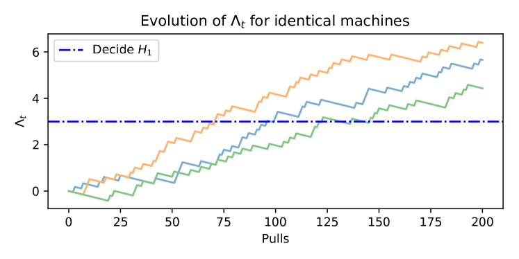
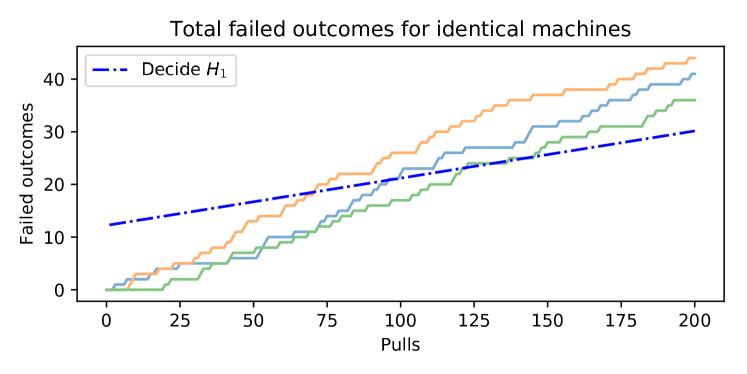
Figure 2: Sequential probability ratio test for $\mu=0.9$, $\epsilon=0.02$, $\alpha=0.05$ and three identical unsafe machines of parameter $\mu_{n}=0.8$. Above: log-likelihood function $\Lambda_{t}$ as a function of the number of pulls of each machine. Below: failed outcomes for each machine as a function of the number of pulls. The test terminates when the sequence surpasses either rejection line (in blue). All three unsafe machines are discarded in finite time.

VI-A Experiment 1: Transient behavior

We consider a setup of $N=1000$ arms, and set a safety guarantee $\mu=0.9$ and a gap $\epsilon=0.05$. The true parameter of each arm is sampled from a uniform distribution $\mathcal{U}\left(0.8,1\right)$. We run sixteen instances of the Safety Inspector described in Algorithm 2 on this test-bed, and then average the results obtained. We define the normalized handicap as the average handicap over all the available arms: $\text{NHandicap}_{t}=\frac{1}{N}\text{Handicap}_{t}$. Figures 3 and 4 show the evolution of the normalized handicap and safety ratio for different tolerance levels $\alpha$, along with the bounds obtained in Theorem 2. Notice that both the handicap and safety ratio remain constant after some time, which indicates that all unsafe machines have been identified, and that no more safe machines are discarded along the way. The final handicap obtained is essentially the number of pulls over all unsafe arms. This is depicted more closely in Figure 5, which presents a histogram of the testing time on unsafe machines, for the setup explained above and for fixed $\alpha=0.1$. Most machines yield a testing time that is strictly lower than the bound in (8). It is important to remark that this bound is on the expected time, and therefore a small number of machines actually need to be tested for longer. Nevertheless, the empirical mean represented by a dashed green line in Fig. 5 lies below the red line that represents the bound. This bound, as well as those in Figs. 3 and 4, is loose because the machines parameters $\mu_{n}$ were drawn uniformly from $\mathcal{U}\left(0.8,1\right)$, but becomes tight if selected as the limiting parameters of the hypothesis test $\mu_{n}\in\{\mu,\mu+\epsilon\}$.

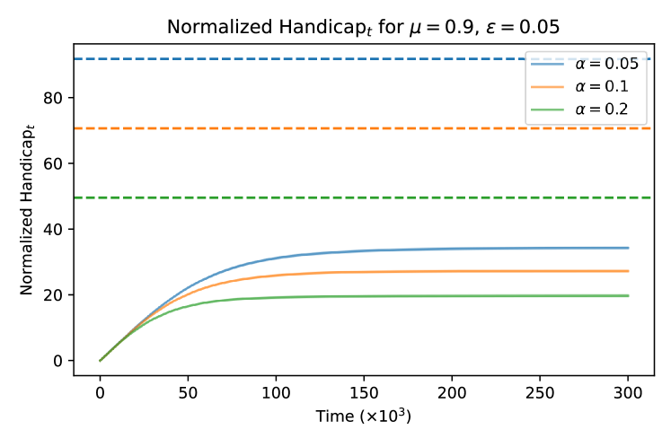
Figure 3: Evolution of the Normalized Handicap through training for $\mu=0.9$, $\epsilon=0.05$ and machines with parameter drawn from $\mathcal{U}(0.8,1)$. Each solid line corresponds to the handicap obtained with a different error tolerance $\alpha$, and the dashed lines are the (normalized) bounds on the Handicap (see (31)). All unsafe machines are eventually discarded after sufficient training, and therefore the handicap remains constant.

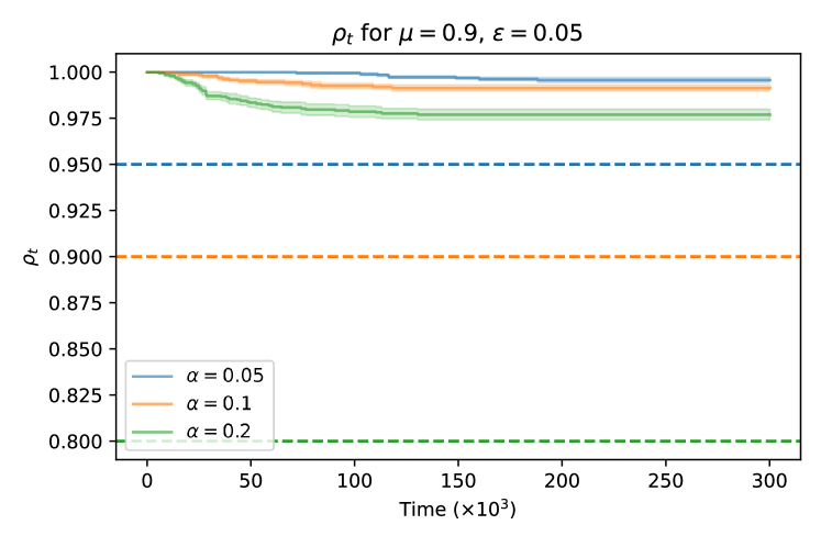
Figure 4: Evolution of the safety ratio $\rho_{t}$ through training for $\mu=0.9$, $\epsilon=0.05$ and machines with parameter drawn from $\mathcal{U}(0.8,1)$, for different tolerance levels $\alpha$. Each solid line is accompanied by its corresponding bound (see (32)).

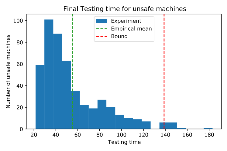
Figure 5: Histogram of the testing time needed to discard unsafe machines, for $\mu=0.9$, $\epsilon=0.05$, $\alpha=0.1$ and machines’ parameters drawn from $\mathcal{U}(0.8,1)$. In dashed red: bound on the testing time from Theorem 2. Since this bound is on the expected testing time, some machines need to be tested for longer. In dashed green: Empirical mean testing time, which is strictly lower than the bound described.

VI-B Experiment 2: Steady state behavior

Repeating the same setup as in Experiment 1, now we perform multiple runs for varying $\epsilon$. Let us define $\text{NHandicap}_{\infty}$ as the maximal normalized handicap obtained —that is, the normalized handicap when all unsafe machines are discarded. Figure 6 illustrates the dependence of $\text{NHandicap}_{\infty}$ for varying $\epsilon$ and $\alpha$. Larger values of $\alpha$ and $\epsilon$ attain lower handicap, which essentially means that unsafe arms are detected faster. This, however, comes at a price —faster detection necessarily implies discarding safe machines along the way. Figure 7 shows the other side of the coin: the final value of the safety ratio $\rho_{t}$ after all unsafe machines have been discarded, which we dub $\rho_{\infty}$. As $\epsilon$ and $\alpha$ grow, $\rho_{\infty}$ diminishes. The conjunction of these two Figures exemplify the preservation-exploration trade-off inherent to our Algorithm.

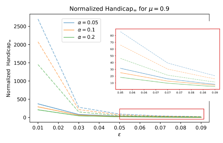
Figure 6: Normalized final Handicap for $\mu=0.9$ as a function of $\epsilon$, for varying tolerance level $\alpha$. As is to be expected, larger values of $\alpha$ and $\epsilon$ achieve lower handicap (which implies faster detection).

Figure 7: Final safety ratio $\rho_{\infty}$ for $\mu=0.9$ as a function of $\epsilon$, for varying $\alpha$. More machines are kept when using small values of $\epsilon$ and $\alpha$, but this in turn implies longer training time (c.f. Figure 6)

VII Conclusions

In this paper we are interested in providing a safety environment for learning. To that end, we advance the idea that detecting if an action is safe is much simpler than trying to estimate its value function, and can be done in finite time. In this direction, we define a measure of handicap that complements the notion of regret by accounting for the aggregate number of unsafe actions explored. We focus on the multi-armed bandit problem, with the goal of detecting the malfunctioning machines and keeping the handicap bounded. For this purpose, we introduced the Relaxed Safety Inspector (Algorithm 2), which we developed as sequential probability ratio test for parallel hypotheses. We proved in Theorem 2 that this algorithm has the property of removing all unsafe machines in finite time, providing a universal bound (33) in terms of the the design parameters $\alpha,\mu$ and $\epsilon$. As a consequence of this, the handicap remains bounded by a finite constant as time goes to infinity. The price to pay for being able to detect all malfunctioning machines in finite time is to accommodate a slack on the machines that are considered safe, and losing a proportion of them. Interestingly, these are design parameters that can be tightened if we are willing to wait longer for detection.

VIII Acknowledgements

The authors thank Hancheng Min and Yue Shen for their comments and valuable suggestions.

References

- [1] K. Zhou, J. C. Doyle, K. Glover, et al., Robust and optimal control, vol. 40. Prentice hall New Jersey, 1996.
- [2] J. O. Berger, Statistical decision theory and Bayesian analysis. Springer Science & Business Media, 2013.
- [3] A. Krizhevsky, I. Sutskever, and G. E. Hinton, “Imagenet classification with deep convolutional neural networks,” in Advances in neural information processing systems, pp. 1097–1105, 2012.
- [4] W. Rawat and Z. Wang, “Deep convolutional neural networks for image classification: A comprehensive review,” Neural computation, vol. 29, no. 9, pp. 2352–2449, 2017.
- [5] G. Hinton, L. Deng, D. Yu, G. E. Dahl, A.-r. Mohamed, N. Jaitly, A. Senior, V. Vanhoucke, P. Nguyen, T. N. Sainath, et al., “Deep neural networks for acoustic modeling in speech recognition: The shared views of four research groups,” IEEE Signal processing magazine, vol. 29, no. 6, pp. 82–97, 2012.
- [6] A. Graves, A.-r. Mohamed, and G. Hinton, “Speech recognition with deep recurrent neural networks,” in 2013 IEEE international conference on acoustics, speech and signal processing, pp. 6645–6649, IEEE, 2013.
- [7] D. Silver, A. Huang, C. J. Maddison, A. Guez, L. Sifre, G. Van Den Driessche, J. Schrittwieser, I. Antonoglou, V. Panneershelvam, M. Lanctot, et al., “Mastering the game of go with deep neural networks and tree search,” nature, vol. 529, no. 7587, p. 484, 2016.
- [8] O. Vinyals, T. Ewalds, S. Bartunov, P. Georgiev, A. S. Vezhnevets, M. Yeo, A. Makhzani, H. Küttler, J. Agapiou, J. Schrittwieser, et al., “Starcraft ii: A new challenge for reinforcement learning,” arXiv preprint arXiv:1708.04782, 2017.
- [9] P. Geibel, “Reinforcement Learning for MDPs with Constraints,” vol. 4212 of Machine Learning: ECML 2006, pp. 646–653, 2006.
- [10] M. Zanon and S. Gros, “Safe Reinforcement Learning Using Robust MPC,” arXiv, 2019.
- [11] S. Paternain, M. Calvo-Fullana, L. F. O. Chamon, and A. Ribeiro, “Safe Policies for Reinforcement Learning via Primal-Dual Methods,” arxiv, 2019.
- [12] R. Cheng, G. Orosz, R. M. Murray, and J. W. Burdick, “End-to-End Safe Reinforcement Learning through Barrier Functions for Safety-Critical Continuous Control Tasks,” arXiv, 2019.
- [13] J. Achiam, D. Held, A. Tamar, and P. Abbeel, “Constrained Policy Optimization,” arXiv, vol. cs.LG, 2017.
- [14] S. Dean, H. Mania, N. Matni, B. Recht, and S. Tu, “On the Sample Complexity of the Linear Quadratic Regulator,” Foundations of Computational Mathematics, vol. 20, no. 4, pp. 633–679, 2020.
- [15] S. Dean, S. Tu, N. Matni, and B. Recht, “Safely Learning to Control the Constrained Linear Quadratic Regulator,” arxiv.
- [16] M. Fazlyab, M. Morari, and G. J. Pappas, “Safety Verification and Robustness Analysis of Neural Networks via Quadratic Constraints and Semidefinite Programming,” arXiv, 2019.
- [17] A. Moradipari, M. Alizadeh, and C. Thrampoulidis, “Linear Thompson Sampling Under Unknown Linear Constraints,” ICASSP 2020 - 2020 IEEE International Conference on Acoustics, Speech and Signal Processing (ICASSP), vol. 00, pp. 3392–3396, 2020.
- [18] S. Amani, M. Alizadeh, and C. Thrampoulidis, “Linear Stochastic Bandits Under Safety Constraints,” arXiv, 2019.
- [19] A. Wald, “Sequential Tests of Statistical Hypotheses,” The Annals of Mathematical Statistics, vol. 2, no. 16, pp. 117—186, 1945.
- [20] T. Lai and H. Robbins, “Asymptotically efficient adaptive allocation rules,” Advances in Applied Mathematics, vol. 6, no. 1, pp. 4–22, 1985.
- [21] Merriam-Webster, “Handicap.”
- [22] T. Lattimore and C. Szepesvári, Bandit algorithms. Cambridge University Press, 2020.