Frequency-dependent magnetic susceptibility of magnetic nanoparticles in a polymer solution: a simulation study
	Patrick Kreissl,∗a Christian Holma and Rudolf Weebera
	Magnetic composite materials i.e. elastomers, polymer gels, or polymer solutions with embedded magnetic nanoparticles are useful for many technical and bio-medical applications. However, the microscopic details of the coupling mechanisms between the magnetic properties of the particles and the mechanical properties of the (visco)elastic polymer matrix remain unresolved. Here we study the response of a single-domain spherical magnetic nanoparticle that is suspended in a polymer solution to alternating magnetic fields. As interactions we consider only excluded volume interactions with the polymers and hydrodynamic interactions mediated through the solvent. The AC susceptibility spectra are calculated using a linear response Green-Kubo approach, and the influences of changing polymer concentration and polymer length are investigated. Our data is compared to recent measurements of the AC susceptibility for a typical magnetic composite system [Roeben et al., Colloid and Polymer Science, 2014, 2013–2023], and demonstrates the importance of hydrodynamic coupling in such systems.

1 Introduction

Magnetic nanoparticles (MNPs) have been connected to many technical applications and are also promising candidates for novel bio-medical treatments. They can be manufactured by splitting larger magnetic objects into smaller particles (e.g. by grinding) or synthesized using chemical processes, allowing for particles of well-defined shape, size, and material properties.^{1, 2, 3, 4, 5, 6, 7, 8, 9} As the human body mass is transparent to static magnetic fields, MNPs that are injected into a body can be moved by application of inhomogeneous external fields. This allows an externally controlled accumulation of MNPs in specific places, e.g. in tumors. Loading the particles with therapeutics before injection, they can be used as a targeted drug delivery system – an important step toward locally constrained chemotherapy.^{10, 11, 12, 13, 14} Another promising approach to cancer treatment based on MNPs is the local heating of cancer cells, so-called ‘hyperthermia’.^{15, 16, 17, 18, 19, 20} Typical bio-medical applications of MNPs will be situated in a polymer-rich, i.e., complex cellular environment. The use of MNPs in a technical context has mainly two aspects. On one hand, they can be embedded in a polymeric gel or suspension to create a soft composite material. The coupling between the magnetic properties of the particles and (visco)elastic properties of the polymer matrix allows for the dynamic control of some aspects of the composite. This includes, e.g., changing their shape, motion, or elastic properties using external fields, which makes them interesting candidates for a variety of applications.^{21, 22, 23, 24, 25, 26, 27, 28} On the other hand, MNPs can be viewed as probes that are used to asses the local behaviour of a polymeric environment. A well established experimental technique for that is the so-called AC susceptometry, where a (sinusoidal modulated) external magnetic field is applied to a sample. Frequency-dependent susceptibility spectra are obtained by simultaneous measurement of the probes’ magnetization response. Besides the insight gained into the magnetic behaviour of the composite as a whole, there exist a number of theoretical models that connect the susceptibility to frequency-dependent mechanical properties. Using, e.g., extended Debye models,^{29, 30, 31} the Gemant-DiMarzio-Bishop model,^{32, 33, 34, 35, 36, 37} or the theoretical model derived by Raikher et al. ³⁸, one may infer the frequency-dependent local viscosity and even elastic moduli on the particle scale, a method dubbed magnetic nanorheology.

A good understanding of the coupling mechanisms is key, when it comes to tailoring the properties of MNPs to a specific bio-medical and technical use case. Unfortunately, often the details of the coupling between the particles and the polymeric environment are not fully known and moreover difficult to (directly) determine experimentally. Here, computer simulations are a powerful tool, allowing the study of well-defined model systems. Aspects of the computational models can be easily modified, where it might be difficult to do so experimentally. Computational models exist on different scales of modelling. While continuum descriptions are well-suited to model MNP–polymer composites on a macro-level,^{39, 40, 41, 42, 43} they typically lack details on the length scale of single polymers. This, however, will be necessary to study how individual changes to the polymer matrix affect its coupling to the embedded MNPs. In this work, we therefore present a particle-based molecular dynamics (MD) simulation model for MNPs immersed in a polymer solution. As explicit resolution of the polymers comes at a high computational cost – in particular at high concentrations and large sample sizes – we focus on the efficient modelling of such systems. The model, which will be presented in section 2, uses coarse-grained polymers, that are coupled to a computationally efficient lattice-Boltzmann hydrodynamics solver; MNPs are modelled as so-called ‘raspberry particles’,^{44, 45} in order to couple translations as well as rotations hydrodynamically to the environment. We use our model to simulate a typical nanorheological system. As a representative example, we use the system of Roeben et al. ⁴ throughout this publication. The parameters required for simulation using our model are specified in section 3. To compare to the experiment, we need to obtain AC susceptibility spectra from the simulations, which can be done in two ways. While the susceptibility can be directly measured for specific frequencies (section 4.2), our main method is based on Green-Kubo linear response theory (section 4.3). It allows us to obtain a complete susceptibility spectrum from a single (however more expensive) simulation. With this approach, we demonstrate that our model reproduces the experimental trends. Using the Green-Kubo approach, we run simulations to illustrate how changes to the polymer matrix affect the resulting susceptibility. Higher values for both, the polymer volume fraction and the polymers’ chain length, are found to independently cause a shift of the susceptibility spectra towards lower frequencies (section 5), which is in accordance with the experimental observations of Roeben et al. ⁴. We end with a discussion of our model and the results obtained our the simulations of the experimental system.

2 Computational model

In this section we present an efficient MD model for simulations of typical nanorheological systems, i.e. (magnetically blocked) MNPs immersed in polymer suspension. Such systems consist of three main components that have to be included in the model, namely the polymers, the fluid, and the magnetic particles.

In MD simulations, parts of the system are represented by interacting MD particles, which are propagated through space and time by time-discrete integration of Newton’s equation of motion. For the polymers, the so-called bead–spring formalism is used. Every polymer chain is explicitly resolved using MD beads, which are inter-connected by an attractive potential – here, we use a simple harmonic interaction of the form

$$\varphi_{\mathrm{harm}}=\frac{1}{2}k(r-r_{0})^{2},$$ (1)

where $r$ is the distance between two consecutive MD beads within a polymer chain, $r_{0}$ is the potential’s equilibrium distance and the spring constant $k$ determines the stiffness of the bond. The MD beads themselves interact via a purely repulsive Weeks-Chandler-Andersen (WCA) potential⁴⁶

$$\varphi_{\mathrm{WCA}}(r)=\begin{cases}\varphi_{\mathrm{LJ}}+\epsilon&\mathrm{if}\ r<2^{1/6}\sigma,\\ 0&\mathrm{otherwise,}\end{cases}$$ (2)

based on the well-known 6-12 Lennard-Jones (LJ) pair potential,

$$\varphi_{\mathrm{LJ}}=4\epsilon\left[\left(\frac{\sigma}{r}\right)^{12}-\left(\frac{\sigma}{r}\right)^{6}\right],$$ (3)

with $\epsilon$ the depth of the LJ potential well and $\sigma$ the distance at which $\varphi_{\mathrm{LJ}}=0$. The repulsive interaction effectively models excluded volume. Note that typically every MD bead within the polymer will represent more than one ‘real-world’ monomer unit. This coarse-graining approach allows for significantly larger system sizes or simulation times as it reduces the number of interacting particles.

To include the hydrodynamic coupling between MNPs and close-by polymers in our model, hydrodynamics are solved using the lattice-Boltzmann (LB) algorithm.^{47, 48} This very efficient grid-based hydrodynamics solver can be straight-forwardly parallelized, has good scaling behaviour, and there also exist fast implementations using graphics cards. Their computational performance make LB algorithms well-suited for the mesoscale. On the small length-scales of our system, thermal fluctuations are an important part of modelling. The LB fluid can be thermalized by adding stochastic fluctuations to the stress tensor, which guarantees local mass and momentum conservation.^{49, 50, 51} To couple MD particles to this fluid, a dissipative friction force is used, which also has to be thermalized. Following Ahlrichs and Dünweg ⁵², the coupling force is given by

$$\vec{F}=-\gamma(\vec{u}_{\mathrm{fluid}}-\vec{u}_{\mathrm{part}})+\vec{\mathcal{F}}.$$ (4)

Its strength is determined by the friction parameter $\gamma$ and the difference of fluid velocity $\vec{u}_{\mathbf{fluid}}$ and velocity of the particle $\vec{u}_{\mathrm{part}}$. Fluctuations are incorporated via the stochastic force $\vec{\mathcal{F}}$ of zero mean and

$$\langle\mathcal{F}_{i}(t)\mathcal{F}_{j}(t^{\prime})\rangle=2\gamma k_{\mathbf{B}}T\delta_{ij}\delta(t-t^{\prime}),$$ (5)

where $\delta$ is the Kronecker delta.

In typical experimental setups, the MNPs are at least one order of magnitude larger than the polymers’ persistence length $\lambda_{\mathrm{p}}$ (e.g., in the experimental system which serves as a basis for the parameter choices in section 3,⁴ $r_{\mathrm{h}}/\lambda_{\mathrm{p}}\approx 18.9$, with hydrodynamic radius $r_{\mathrm{h}}$ of the magnetic particle). To properly capture the hydrodynamic behaviour of the MNPs in the model, it does not suffice to just use a single coupling point per particle. With such an approach every MNP would couple to only a single lattice site per time step, with no rotational coupling. In addition, the hydrodynamic impact of the MNP’s shape would be neglected. Thus, to obtain the physically expected hydrodynamic behaviour, the so-called ‘raspberry model’ is used for the MNPs, which means homogeneously filling their shape with fluid coupling points that are rigidly bound to a central MD bead.⁴⁴ For preparation of the raspberry we follow the procedure described by Fischer et al. ⁴⁵, which we will only briefly sketch here. For in-depth information please consult the referenced publication. Creating the raspberry particle happens in a two-step process: resolving the surface and then homogeneously filling its volume, which is necessary to obtain consistent translational and rotational diffusivities $D_{\mathrm{t}}$ and $D_{\mathrm{r}}$.^{45, 53} The preparation process uses a MD approach. To resolve the surface of the raspberry, (mobile) MD beads are put into an empty simulation box. A harmonic potential (see eq. 5) that is shifted by the desired raspberry radius $r_{0}=r_{\mathrm{rasp}}$, is used to force the beads onto a spherical shell. To homogenize the surface density, a purely repulsive WCA potential (see eq. 2) is added between the MD beads. By slowly increasing the harmonic spring constant $k$ to an extremely high target value, MD beads end up forming a homogeneous surface shell. After correcting small deviations of the beads’ desired distances from the raspberry centre ($|\vec{r}|=r_{\mathrm{rasp}}$), they are rigidly connected to the centre position and the harmonic bonds removed. Now the raspberry can be filled by adding MD beads inside the hollow shell, which interact again via a repulsive WCA potential. To prevent numerical instabilities, the resulting forces are initially capped. The positions of the MD beads are allowed to evolve using MD (with a Langevin thermostat) while slowly raising the force cap. This procedure typically leads to a homogeneous distribution of MD beads, which is tested by tracking the shell-wise particle density, as well as the geometric centre of all raspberry bead positions (it should coincide with the raspberry centre). Once these conditions are fulfilled, the MD beads are rigidly bound to the raspberry centre.⁴⁵ All beads of the resulting raspberry-like shaped rigid body now act as fluid coupling points. They couple to the LB fluid via the same friction force as the other MD beads (see eq. 4). The equation of motion, however, is only integrated for the body’s central bead, which carries the mass $M_{\mathrm{rasp}}$ and moment of inertia $I=2M_{\mathrm{rasp}}r_{\mathrm{rasp}}^{2}/5$ of the particle, as well as its magnetic moment $m$. Figure 1 shows a cut through the raspberry particle used for this publication.

Fig.  1: Cut through the spherical raspberry particle used for this publication. It consists of homogeneously distributed fluid coupling points (blue) forming a rigid body. Newton’s equation of motion is integrated only for its centre (black), which carries the particle’s mass, as well as its magnetic moment (indicated by the yellow arrow).

Imposing a meaningful potential between the central bead and polymer MD particles, one can model respective interactions – as we will see in section 3, we choose a purely repulsive WCA potential, here, but more involved interaction potentials would also be possible. Note that for a spherical particle these interactions can only lead to translations. Coupling of the rotational behaviour happens only via hydrodynamics which are thus essential to our model.

3 Model parameters

To establish a close relationship between experiment and modelling, we set up simulations based on the experimental system used by Roeben et al. ⁴ and Hess et al. ⁵⁴ for nanorheological measurements. It consists of spherical, magnetically blocked single-domain cobalt ferrite (CoFe2O4) nanoparticles immersed in an aqueous polyethylene glycol (PEG) solution. The CoFe2O4 particles act as probes for investigating the nanorheological properties of the polymer solution. Their magnetic moment is small, and they are used at very high dilutions ($3.6\text{\times}{10}^{-2}\text{\,}\mathrm{\char 37\relax}$ volume fraction⁴). Therefore, dipolar interactions between the MNPs do not play a major role (for an estimate of their relative strength see the calculation of $\lambda$ in section 5). Consequently, we neglect dipolar interactions in our model. This allows us to simulate only a portion of the system containing a single magnetic particle. Periodic boundary conditions are used to eliminate boundary effects, but with a very large simulation box to minimize hydrodynamic interactions between the MNP and its periodic images.

All simulations for this publication were performed using the MD software package ESPResSo.⁵⁵ This software uses the concept of simulation units, that allows the user to freely choose the mass, length, and energy scales of the system, which in combination determine the simulated time scale. For reference, the values of important quantities describing the system are summarized in table 1 using both, SI and simulation units, respectively.

The length scale in our model is prescribed by the hydrodynamic radius of the raspberry particle $r_{\mathrm{rasp}}$, which corresponds to the experimental value of $r_{\mathrm{h}}=$7.2\text{\,}\mathrm{nm}$$.⁴ As simulation domain, we use a cubical box with side length $L_{\mathbf{box}}=10r_{\mathrm{rasp}}$.

Table 1: Overview of the parameters we use for the simulation unit system, for some characteristic system quantities.

Quantity	Value (SI units)	Value (simulation units)
particle radius $r_{\mathrm{rasp}}$	$7.2\text{\,}\mathrm{nm}$	$4\text{\,}\mathrm{[}\mathrm{x}\mathrm{]}$
thermal energy	$k_{\mathrm{B}}$ $\cdot$ $300\text{\,}\mathrm{K}$	$1\text{\,}\mathrm{[}\mathrm{E}\mathrm{]}$
solvent density $\rho_{\mathrm{w}}$	$1\text{\times}{10}^{3}\text{\,}\mathrm{kg}\text{\,}{\mathrm{m}}^{-3}$	$1\text{\,}\mathrm{[}\mathrm{m}\mathrm{]}\mathrm{/}\mathrm{[}\mathrm{x}\mathrm{]}\mathrm{{}^{3}}$
kinematic viscosity $\nu$	$8.9\text{\times}{10}^{-8}\text{\,}{\mathrm{m}}^{2}\text{\,}{\mathrm{s}}^{-1}$	$1.86\text{\,}\mathrm{[}\mathrm{x}\mathrm{]}\mathrm{{}^{2}}\mathrm{/}\mathrm{[}\mathrm{t}\mathrm{]}$
mass unit	$5.8\text{\times}{10}^{-24}\text{\,}\mathrm{kg}$	$1\text{\,}\mathrm{[}\mathrm{m}\mathrm{]}$
time unit	$67.4\text{\,}\mathrm{ps}$	$1\text{\,}\mathrm{[}\mathrm{t}\mathrm{]}$

The energy scale is given by the thermal energy of the system. As the experiments are performed at $T_{\mathrm{exp}}=$25\text{\,}\mathrm{\SIUnitSymbolCelsius}$$, we use $T=$300\text{\,}\mathrm{K}$$ in our model, prescribing the energy scale $$1\text{\,}\mathrm{[}\mathrm{E}\mathrm{]}$=k_{\mathrm{B}}\cdot$300\text{\,}\mathrm{K}$$.

For the fluid, we make the following choices: the size of the LB grid cells is set to $a_{\mathrm{grid}}=$1\text{\,}\mathrm{[}\mathrm{x}\mathrm{]}$=r_{\mathrm{rasp}}/4$ yielding $[x]=$1.8\text{\,}\mathrm{nm}$$; LB fluid density is set to $1\text{\,}\mathrm{[}\mathrm{m}\mathrm{]}\mathrm{/}\mathrm{[}\mathrm{x}\mathrm{]}\mathrm{{}^{3}}$ corresponding to water density $\rho_{\mathrm{w}}=$1\text{\times}{10}^{3}\text{\,}\mathrm{kg}\text{\,}{\mathrm{m}}^{-3}$$, thereby also defining the mass scale $[m]=$5.8\text{\times}{10}^{-24}\text{\,}\mathrm{kg}$$. For the magnetic particle, we use the bulk density of CoFe2O4, $\rho_{\ce{CoFe2O4}}=$5.3\text{\times}{10}^{3}\text{\,}\mathrm{kg}\text{\,}{\mathrm{m}}^{-3}$$.⁵⁶ We make a simplifying assumption concerning the fluid viscosity by choosing its value as one tenth the experimental kinematic viscosity of water, $\nu_{\mathrm{exp}}=0.1\nu_{\mathrm{w}}=$8.9\text{\times}{10}^{-8}\text{\,}{\mathrm{m}}^{2}\text{\,}{\mathrm{s}}^{-1}$$,⁵⁷ in simulation units $\nu=$1.86\text{\,}\mathrm{[}\mathrm{x}\mathrm{]}\mathrm{{}^{2}}\mathrm{/}\mathrm{[}\mathrm{t}\mathrm{]}$$. This effectively decreases the decay time of the magnetic moment of the MNP through rotational motion, which reduces simulation time by roughly one order of magnitude. Per every MD time step $\Delta t=$0.01\text{\,}\mathrm{[}\mathrm{t}\mathrm{]}$$, the LB fluid field is updated. The simulated time scale is fully determined by the prescribed length, energy, and mass scales yielding $[t]=$67.4\text{\,}\mathrm{ps}$$.

In the experiment, PEG is the polymer species being used. Experimentally, the mean monomer length in PEG is $2.78\text{\,}\mathrm{\SIUnitSymbolAngstrom}$,⁵⁸ the chain’s persistence length in aqueous solution $\lambda_{\mathrm{p}}\approx$3.8\text{\,}\mathrm{\SIUnitSymbolAngstrom}$$.^{59, 60} To accurately capture the experimental size ratio between magnetic particles and persistence length of PEG would be computationally exceedingly demanding, limiting investigations to small polymer concentrations or simulation times. Our aim is, however, to end up with a computationally model that can handle polymer volume fractions up to as high as $\sim$25\text{\,}\mathrm{\char 37\relax}$$. In addition, simulations of such systems have to capture both, the relaxation time of the polymer suspension and the relatively long self-diffusion time of the magnetic particle, making coarse-graining of the polymers indispensable. While this may change the strength of some effects in the system, general trends are expected to remain unaffected – for results and discussion, please see section 4. As water is a good solvent for PEG, excluded volume has to be considered for the polymers, which is accounted for using a purely repulsive WCA interaction between monomer beads (see eq. 2). The diameter of the monomer beads is given by the choice of the WCA parameter, here $\sigma_{\mathrm{mono}}=$1\text{\,}\mathrm{[}\mathrm{x}\mathrm{]}$$; we set $\epsilon_{\mathrm{mono}}=$1\text{\,}\mathrm{[}\mathrm{E}\mathrm{]}$$. The equilibrium length of the harmonic potential which connects monomer beads within each polymer chain (eq. 5) is set to $r_{0}=\sigma_{\mathrm{mono}}$, the spring constant $k=$200\text{\,}\mathrm{[}\mathrm{E}\mathrm{]}\mathrm{/}\mathrm{[}\mathrm{x}\mathrm{]}\mathrm{{}^{2}}$$. Finally, to prevent polymers from penetrating the ‘solid’ MNP, an additional WCA potential is required between the monomer beads of the polymers and the raspberry particle. In principle, this interaction could be set between monomer beads and the coupling points of the raspberry. Since, in general, the coupling points do not smoothly resolve the raspberry surface, any remaining surface roughness introduces additional rotational coupling. As detailed in section 2, using the raspberry model the main concern is to obtain consistent translational and rotational diffusive behaviour for the MNP, which can be challenging in itself and does in no way guarantee a smooth resolution of the MNP’s surface. To avoid artefacts in the rotational coupling, we therefore prescribe the repulsive WCA potential between the monomer beads and the centre or the raspberry particle. The parameters for this mixed interaction are $\epsilon_{\mathrm{mix}}=$1\text{\,}\mathrm{[}\mathrm{E}\mathrm{]}$$ and $\sigma_{\mathrm{mix}}=(r_{\mathrm{rasp}}+\sigma_{\mathrm{mono}}/2)$. The raspberry used for this publication consists of 1400 coupling points ($\approx 5.25$ per LB unit cell), the fluid-coupling friction parameter is $\gamma=$15\text{\,}\mathrm{[}\mathrm{m}\mathrm{]}\mathrm{/}\mathrm{[}\mathrm{t}\mathrm{]}$$. A visualization of the raspberry is given in figure 1, a representative snapshot of the readily set-up system is shown in figure 2.

Fig.  2: Visualization of the simulation model described in section 2 using the parameters of section 3. Raspberry coupling points are colored blue, (coarse-grained) polymers green. Here, each polymer chain consists of 15 beads. For visibility reasons, the polymer volume fraction in the shown setup is only $\phi=0.01$. Typical volume fractions used for our simulations are significantly higher, up to $\phi=0.25$.

4 Obtaining AC susceptibility spectra from simulations

The AC susceptibility is the differential response of a system’s magnetization $M(t)$ to an oscillating external magnetic field $H(t)$, i.e. $\chi=\mathrm{d}M(t)/\mathrm{d}H(t)$. The result is a complex value $\chi=\chi^{\prime}-\textit{i}\chi^{\prime\prime}$.

4.1 For reference: Debye model

Before introducing the methods for measuring AC susceptibility spectra in the simulation, we briefly present the result of the theoretical Debye model.⁶¹ It was first derived by Debye (1929), originally to describe the relaxation of the rotational polarization of molecules, but generally captures the rotational relaxation process of any dipole. The model makes a few assumptions. Namely, it describes the magnetization of non-interacting ideal dipoles that couple to a fluid with frequency-independent dynamic viscosity $\eta=\nu\rho$ via rotational Stokes friction $\zeta_{\mathrm{r}}=8\pi\eta r^{3}$. The magnetic susceptibility analytically evaluates to

$$\chi(\omega)=\frac{\chi_{0}}{1+\mathrm{i}\omega\tau},$$ (6)

with $\chi_{0}$ the zero-frequency susceptibility and $\tau$ the characteristic decay time of the magnetic moment.

For a raspberry particle in a LB fluid, as used in our model, these assumptions are fulfilled. We can therefore use the Debye model as a reference curve to benchmark our measurement techniques against. In our model we consider magnetically blocked particles only and thus do not allow internal (Néel-)relaxation of the magnetic moment. Instead, decorrelation of the orientation of the dipole moment only happens via (rotational) Brownian diffusion. As a result we have

$$\tau=\tau_{\mathrm{B}}=\frac{3\eta V_{\mathrm{h}}}{k_{\mathrm{B}}T},$$ (7)

with Boltzmann’s constant $k_{\mathrm{B}}$, temperature $T$, and the hydrodynamic volume $V_{\mathrm{h}}=4\pi r_{\mathrm{h}}^{3}/3$.⁶¹

4.2 Direct measurement

The straightforward approach of measuring the AC susceptibility of the simulation is by faithfully reproducing the experimental measurement technique i.e. measuring per frequency $f$: for any chosen angular frequency $\omega=2\pi f$, a time-dependent alternating magnetic field

$$\vec{H}(t)=\vec{H}_{0}\sin(\omega t),$$ (8)

with amplitude $\vec{H}_{0}$ is explicitly applied to the simulation box, causing a torque on the magnetic particle. The magnetization response of the system is measured via the component of the particle’s magnetic moment that points into field direction.

For weak coupling to the external field, the magnetization $\vec{M}(t)$ will also have a sinusoidal shape

$$\vec{M}(t)=\vec{M}_{\mathrm{max}}\sin(\omega t-\vartheta),$$ (9)

but with a frequency-dependent phase shift $\vartheta$. However, this signal will be superimposed by thermal noise. To bring out the signal, averaging over several periods is necessary, as will be discussed shortly.

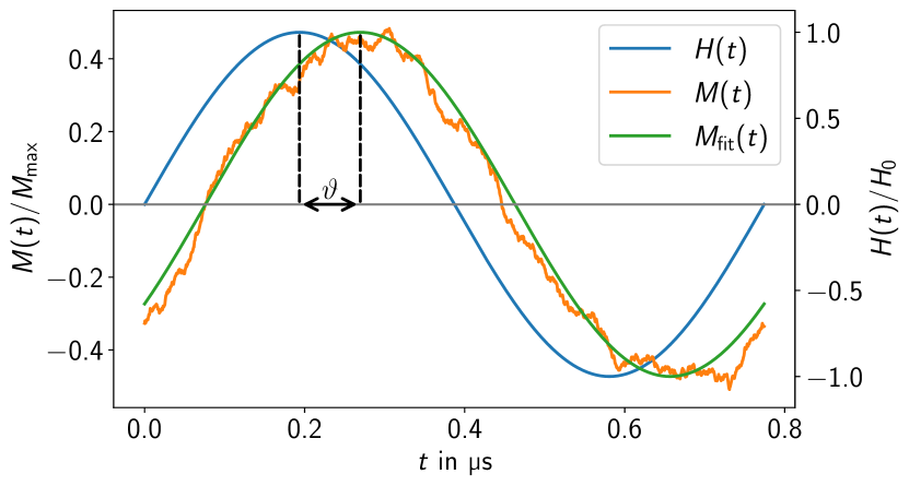
Fig.  3: Direct measurement of the susceptibility: an external magnetic AC field $H$ (frequency $f=$1\,291\,549\text{\,}\mathrm{Hz}$$) is applied to the system and its magnetization response $M(t)$ is measured. Due to Brownian diffusion this signal will be noisy and has thus to be averaged over several periods, 64 here. The mean magnetization (orange) is then fitted (green, for functional form see eq. 9) to obtain the phase shift $\theta$.

The phase shift is then used to obtain the complex magnetic susceptibility $\chi=M(t)/H(t)=\chi^{\prime}-\mathrm{i}\chi^{\prime\prime}$, where the real part $\chi^{\prime}$, that relates to reversible magnetization, is in phase with the external field. The imaginary component $\chi^{\prime\prime}$ is related to losses and can be computed as the out-of-phase part of the magnetization response. We get

$$\chi^{\prime} =\frac{M_{\mathrm{max}}}{H_{0}}\cos\left(\vartheta\right),$$ (10)

$$\chi^{\prime\prime} =\frac{M_{\mathrm{max}}}{H_{0}}\sin\left(\vartheta\right).$$ (11)

A visualization of the analysis is shown in figure 3. Exemplary results of such direct measurements for a MNP in a Newtonian fluid are shown in figure 4. For reference, the corresponding Debye model result is also shown. The positions of imaginary susceptibility peaks match quite well. The same is true for the real part of the susceptibility in that region. There are, however, some deviations from the curve predicted by Debye. This can be attributed to the non-linear nature of the Langevin magnetization law.^{62, 63} Typically, the so-called Langevin parameter is used to characterize the magnetic interaction strength. The Langevin parameter

$$\alpha=\frac{\mu_{0}mH}{k_{\mathrm{B}}T}$$ (12)

compares the magnetic interaction energy between the particle’s dipole $m$ and the field to the thermal energy. Here, $\mu_{0}$ is the magnetic constant. In order to minimize non-linear effects in the susceptibility spectra, one would like to choose $\alpha\ll 1$. However, choosing a low $\alpha$ simultaneously increases the relative importance of thermal fluctuations in the system – the signal-to-noise ratio drops significantly, which means much longer simulation times are necessary for comparable statistics. Minimizing non-linear effects when using direct measurements thus comes at a high computational cost. Another obvious shortcoming of this technique is that each simulation yields the complex susceptibility only for the chosen frequency $\omega$. To sample complete susceptibility spectra with high resolution is therefore hardly feasible. However, direct measurements may come in handy when observing interesting behaviour at specific frequencies.

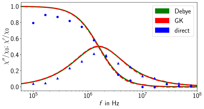
Fig.  4: AC susceptibility spectra measured from the simulation of a MNP in a Newtonian fluid without any polymers. Blue data points are results of direct measurements (Langevin parameter $\alpha=2$). For reference, the theoretical Debye model is shown (green).The spectrum obtained using the Green-Kubo approach (red) matches the theoretical model quite accurately.

4.3 Green-Kubo approach

In this section, we discuss an approach that allows one to obtain the full AC susceptibility spectrum from a single simulation, assuming that the applied external magnetic field is small. In general, the dynamic response of a magnetic suspension to an applied magnetic field is non-linear. However, for small fields, $\alpha\ll 1$, linear response can be assumed. In the framework of linear response theory, the so-called Green-Kubo relations are a general type of fluctuation-dissipation theorems that connect physical quantities such as polarization or complex conductivity to time correlation functions of associated dynamic variables.⁶⁴ Also for the magnetic susceptibility one such Green-Kubo relation can be derived. It reads

$$\chi(\omega)=\frac{1}{Vk_{\mathrm{B}}T}\left[\langle\vec{M}(0)\vec{M}(0)\rangle-\mathrm{i}\omega\int_{0}^{\infty}\exp(-\mathrm{i}\omega t)\langle\vec{M}(t)\vec{M}(0)\rangle\,\mathrm{d}t\right],$$ (13)

where $V$ is the system’s volume. The integral part of this equation is the Fourier-Laplace transform of the time. Applying this relation, a full AC susceptibility spectrum can be directly obtained from one single steady-state simulation (without an explicit external magnetic field).

As this approach solely relies on the auto-correlation of the magnetic moment as an input, one has to make sure that this quantity is well sampled even for large lag times. As a consequence, simulation runs have to be significantly longer than with the direct method. At this point, the simplifications in the used parameter set (decreased viscosity and water density for the magnetic particle) significantly decrease computation time by speeding up the decorrelation of the magnetic moment. Still, in practice, dealing with the integral part can be challenging, as thermal noise in the long-time tail of the auto-correlation function of the magnetic moment is amplified by the frequency. For infinite runs noise in the long-time tail would cancel, leaving a pure decay signal. A common approach to mitigate the impact of tail noise is thus to fit an analytic expression for the tail – a typical choice would be a simple exponential decay,

$$f_{\mathrm{fit}}(t)=\langle\vec{M}(0)\vec{M}(0)\rangle_{\mathrm{fit}}\exp\left(-\frac{t}{\tau_{\mathrm{fit}}}\right),$$ (14)

with $\langle\vec{M}(0)\vec{M}(0)\rangle_{\mathrm{fit}}$ the zero-frequency limit of the magnetization correlation and characteristic decay time $\tau_{\mathrm{fit}}$. Note that depending on the system, more involved functional descriptions may be required to properly capture the decay behaviour, such as the expression for an isolated particle in a viscoelastic medium derived by Ilg and Evangelopoulos ³⁴. Deviations from a pure exponential decay behaviour are also expected for interacting and polydisperse ferrofluid systems.⁶⁶ For our setup, the decay behaviour of the long-time tail is actually well captured using the simple exponential decay. For the well-sampled low-frequency region the numerical data is kept, whereas the fitted function is used for the long-time tail. Between these two regions a smooth transition is made over a certain frequency range. The merged data is given by

$$\langle\vec{M}(t)\vec{M}(0)\rangle=f_{\mathrm{t}}(t)\langle\vec{M}(t)\vec{M}(0)\rangle_{\mathrm{num}}+[1-f_{\mathrm{t}}(t)]f_{\mathrm{fit}}(t),$$ (15)

where $f_{\mathrm{t}}(t)$ is a linear transition function over the interval $[\tau_{\mathrm{l}},\tau_{\mathrm{u}}]$,

$$f_{\mathrm{t}}(t)=\begin{cases}1&t\leq\tau_{\mathrm{l}},\\ (\tau_{\mathrm{u}}-t)/(\tau_{\mathrm{u}}-\tau_{\mathrm{l}})&\tau_{\mathrm{l}}<t<\tau_{\mathrm{u}},\\ 0&t\geq\tau_{\mathrm{u}}.\end{cases}$$ (16)

For a visualization of this procedure see figure 5.

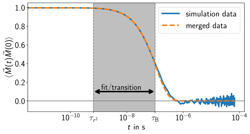
Fig.  5: Representative example for the time auto-correlation function of the magnetization obtained from our simulation model (blue solid line). Here, a MNP in a Newtonian fluid was used. To get rid of the Brownian noise in the long-time tail, an analytic exponential function is fitted to the data, the fit region is the indicated grey area. The same frequency range is used to linearly transition from the numerical correlation data to the analytical tail fit (see eqs. 15 and 16). The resulting correlation function is shown by the orange dashed line.

Here, we decided to choose the same time range for fitting and the linear transition between numerical data and analytical tail. As lower boundary ($\tau_{\mathrm{l}}$), we use the viscous time of our system $\tau_{r^{2}}=\rho_{\mathrm{w}}r_{\mathrm{rasp}}^{2}/\eta=$0.58\text{\,}\mathrm{ns}$$ (the time it takes fluid momentum to diffuse by one colloidal radius).^{45, 65} As upper limit ($\tau_{\mathrm{u}}$), we choose the Brownian relaxation time of the Newtonian system $\tau_{\mathrm{B}}=$100.8\text{\,}\mathrm{ns}$$, see equation 7.

The integral in eq. 13 can then be efficiently computed via the Fourier-Laplace-transform of resulting auto-correlation function of the magnetization. The result of such a Green-Kubo susceptibility measurement on a magnetic particle in a Newtonian fluid is shown in figure 4. It perfectly matches the expected theoretical Debye relaxation reference curve.

5 Results and discussion

Using our modeling approach (section 2) with the parameters of section 3 – based on the experimental system of Roeben et al. ⁴ – we set up simulations to study the signatures that changes to the polymeric surroundings generate in the measured susceptibility spectra. Here, we will focus on the effects of (1) varying the polymer volume fraction and (2) the polymer chain length.

To obtain full AC susceptibility spectra, we use the Green–Kubo approach described in section 4.3, which by default operates in the linear response limit. The linear response assumption also holds in the experiment as we can see from the estimated experimental Langevin parameter. With field amplitude $H_{0,\mathrm{exp}}=$0.4\text{\,}\mathrm{kA}\text{\,}{\mathrm{m}}^{-1}$$,⁴ temperature $T_{\mathrm{exp}}=$25\text{\,}\mathrm{\SIUnitSymbolCelsius}$$, and magnetic moment of the particle $m=$3.6\text{\times}{10}^{-19}\text{\,}\mathrm{A}\text{\,}{\mathrm{m}}^{2}$$,⁵⁴ we obtain

$$\alpha_{\mathrm{exp}}=\frac{m\mu_{0}H_{0,\mathrm{exp}}}{k_{\mathrm{B}}T_{\mathrm{exp}}}\approx 0.044\ll 1,$$ (17)

which confirms that the experiments do indeed take place in the linear response limit. For magnetically blocked particles the magnetic moment scales with the particles’ core volume, $m\sim r_{\mathrm{rasp}}^{3}$ (assuming constant thickness of surface coating if present). As the used value was actually measured for a CoFe2O4 particle with hydrodynamic radius $r_{\mathrm{h}}=$10.7\text{\,}\mathrm{nm}$$ (instead of our $r_{\mathrm{h}}=$7.2\text{\,}\mathrm{nm}$$),⁵⁴ we even overestimate the Langevin parameter $\alpha_{\mathrm{exp}}$, here.

With these parameters, we also estimate the relative strength of inter-particle dipolar interactions using the dipolar interaction parameter

$$\lambda=\frac{\mu_{0}m^{2}}{4\pi(2r_{\mathrm{rasp}})^{3}k_{\mathrm{B}}T},$$ (18)

which compares the per-particle dipolar energy for two touching particles in head-to-tail configuration to the thermal energy. We obtain $\lambda_{\mathrm{exp}}\approx 0.25$, a value that indicates rather small dipolar interactions (for particles to show notable structure, one would expect a $\lambda$ larger than $\sim 2$). Particle–particle interactions become important for sufficiently high densities of MNPs and strength of dipolar interactions.^{66, 67, 68, 69} Here, however, the low dipolar interaction parameter and volume fraction ($<$1\text{\,}\mathrm{\char 37\relax}$$) imply that particle–particle interactions do not significantly influence the susceptibility. This justifies our approach of studying a single magnetic particle in its surrounding.

We start with simulations of varying polymer volume fraction. The polymer volume fraction refers only to the polymer solution, i.e., it ignores the volume of the magnetic particles. In general, the polymer volume fraction is thus given by

$$\phi=\frac{N_{\mathrm{poly}}N\left(\frac{\sigma_{\mathrm{mono}}}{2}\right)^{3}}{\frac{3}{4\pi}V_{\mathrm{box}}-N_{\mathrm{rasp}}r_{\mathrm{rasp}}^{3}},$$ (19)

with number of polymers $N_{\mathbf{poly}}$, monomer units per polymer $N$, and the radius per monomer unit $\sigma$ (to calculate its excluded volume). The box volume is given by $V_{\mathrm{box}}$, $N_{\mathrm{rasp}}$ is the number of raspberries with radius $r_{\mathrm{rasp}}$ inside the box. For the parameters used in our simulations, see section 3. To study the effect of increasing polymer concentrations, we choose a constant chain length of $N=15$ and systematically vary the volume fraction $\phi\in\{0.05,\,0.15,\,0.25\}$. The magnetic moment of the particle is recorded every $0.1$ time unit (every $6.7\text{\,}\mathrm{ps}$). The total number of samples per simulations run is $N_{\mathrm{samples}}=$2\text{\times}{10}^{7}\text{\,}$$. The resulting susceptibility spectra are shown in figure 6.

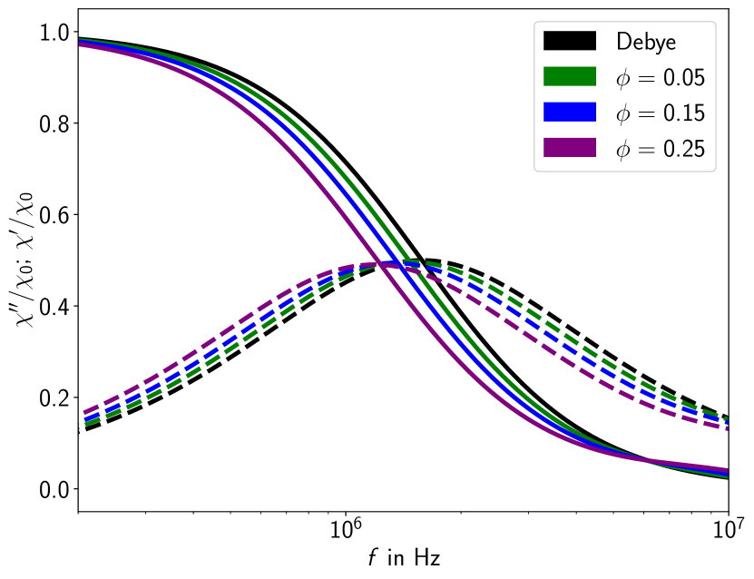
Fig.  6: The AC susceptibility spectra obtained from simulations with polymers of chain length $N=15$ at different volume fractions. Increasing the polymer volume fraction leads to a shift towards lower frequencies. Solid lines indicate the real, dashed lines the imaginary part of the susceptibility.

With increasing polymer fraction, the susceptibility curves experience a shift towards lower frequencies. As the Debye shape of the curve is preserved for all cases, these shifts signify an increase of the effective viscosity around the MNP. Even at the highest concentration, no entanglement of polymers is expected – as will be discussed shortly, both polymer length and volume fraction would have to be considerably higher.

Let us now turn to the simulations at a constant volume fraction $\phi=0.25$ where the polymer chain length is systematically varied $N\in\{1,\,5,\,15,\,25\}$. Results are shown in figure 7. Again, a shift of the measured spectra towards lower frequencies is observed while maintaining the Debye shape, where larger shifts occur with increasing chain length.

Fig.  7: AC susceptibility spectra for magnetic particles in solution with volume fraction of polymers $\phi=0.25$. The chain length of the polymers $N$ is varied. The longer the chains are, the more the spectra get shifted towards lower frequencies. Solid lines indicate the real, dashed lines the imaginary part of the susceptibility. The inset shows the corresponding fitted relaxation times $\tau_{\mathrm{fit}}$.

It can be seen from the figure, that already the addition of unconnected monomers causes a significant shift in frequency. In our computational model, the monomer beads are coupled to the fluid via the thermalized friction force of equation 4, thus slowing down fluid dynamics. This registers as an increased effective fluid viscosity, causing a higher relaxation time for the systems’ magnetization. An overview of the relaxation times obtained via fitting the long-time tail (section 4.3) can be found in table 2.

Table 2: Overview of the zero-frequency magnetization correlations and decay times fitted using the procedure described in section 4.3, for simulations at different polymer volume fraction $\phi$ and number of monomers per chain $N$.

$\phi$	$N$	$\langle\vec{M}(0)\vec{M}(0)\rangle_{\mathrm{fit}}$	$\tau_{\mathrm{fit}}/\tau_{\mathrm{B}}$
0.00	0	1.00	1.010
0.05	15	0.99	1.089
0.15	15	0.99	1.185
0.25	1	0.99	1.216
0.25	5	0.99	1.240
0.25	15	0.98	1.333
0.25	25	0.98	1.373

By increasing both, the length of polymers and their concentration, this purely hydrodynamic effect is intensified through the increased coupling to the polymer matrix. The observed behaviour matches the experimental observations of Roeben et al. ⁴ In the experiment, PEG solutions with different chain lengths and polymer concentrations were studied. As in our simulation results, for low polymer fractions (depending on the chain length) the experimentally measured susceptibility spectra are simple Debye-type curves with a single relaxation time, which directly depends on the effective viscosity of the polymer suspension. With increasing PEG concentration and chain length, however, the experimentally measured spectra broaden and some measurements also suggest the existence of a second relaxation process.⁴ The emerging deviation from Newtonian behaviour is most noticeable above the overlap concentration of the respective solution. This indicates entanglement of polymer chains as a main cause. The broadening of Debye spectra for spherical MNPs in increasingly elastic environments was also observed by other experimental groups.⁵

To get a feeling for the polymer lengths required to observe entanglement in the simulation model, the work of Kremer and Grest ⁷⁰ on polymer melts may serve as an indication. Using a FENE potential (instead of harmonic) to connect the MD beads within polymers and a slightly different parameter set, they found an entanglement length of $N_{\mathrm{e}}=35$ at a volume fraction of $\phi=0.45$.⁷⁰ In our simulations we are well below these values, with maximum $N=25$ and $\phi=0.25$. Despite the deviations in modelling, we thus expect that polymer chains would have to be significantly longer and used at higher volume fractions before seeing effects of entanglement.

As already described, our model makes several simplifying assumptions such as the use of coarse-grained polymers and using one tenth the viscosity of water for our fluid. Our results are therefore not expected to quantitatively reproduce the experimental findings. To get an idea of the relative strength of the effects in the experiment and simulation, let us make a rough comparison, neglecting polymer entanglement effects. In the simulations we found that the use of polymers of length $N=25$ at a polymer volume fraction of $\phi=0.25$ leads to an increase of the relaxation time by $\sim$37\text{\,}\mathrm{\char 37\relax}$$. Experimentally, the use of $25\text{\,}\text{vol.-}\mathrm{\char 37\relax}$ PEG increased the dynamic viscosity and thus the relaxation time (see eq. 7, we are in the Debye-like Newtonian limit) by roughly a factor of $2$ for triethylene glycol and about a factor of $3$ for PEG1000.⁴ The effect observed in the simulations is thus roughly one order of magnitude smaller than in the experiment, possibly due to the small length of our polymers (compared to PEG1000), and the neglect of any specific interactions of the polymers with the MNPs.

As a key result, our simulations show the importance of hydrodynamics for magnetic composite systems. Since all pair interactions between the MNP and surrounding monomer beads just affect the particle’s translational behaviour, hydrodynamic interactions are the only possible source of rotational coupling. Our simulations demonstrate that this is already sufficient to qualitatively reproduce the experimentally observed shifts of the AC susceptibility spectra towards lower frequencies for both, higher polymer volume fractions and longer chains, respectively.

6 Conclusions

In this work, we presented a simulation model for magnetic nanoparticles in polymer suspensions and showed how frequency-dependent AC susceptibility spectra can be obtained from the simulations. Our modelling approach is based on molecular dynamics, coupled to an efficient lattice-Boltzmann hydrodynamics solver. While still costly, we managed to bring the computational complexity down to a feasible level. To do so, we made some simplifying assumptions, such as a certain level of coarse-graining regarding the polymers. Using our model, we ran simulations with parameters based on the experimental system of Roeben et al. ⁴, to study the signatures that changes to the polymeric surroundings produce in the resulting susceptibility spectra. For this, we simulated a single particle in its polymeric environment (using periodic boundary conditions). This is justified because of the low concentration of particles as well as small dipolar interaction strength in the experimental system. We presented two approaches to obtain susceptibility spectra from our simulations. Using direct measurement one may obtain the susceptibility for a specific frequency, which, however, is quite costly when it comes to sampling entire spectra over a large range of frequencies. We therefore introduced a second approach based on Green-Kubo linear response theory. To benchmark this method with our model, we showed that the simulation of a particle in a Newtonian fluid reproduces the curve expected from Debye relaxation theory. We used the Green-Kubo approach throughout our simulation study of a spherical nanoparticle in a polymer suspension. Matching the experimental observations,⁴ we found that the AC susceptibility spectra are shifted towards lower frequencies,⁴ when either increasing the polymer volume fraction or the polymer chain length for a fixed polymer concentration. In our model, hydrodynamic interactions provide the sole source of direct coupling between the polymeric environment and the rotational behaviour of the particle, i.e. the Brownian relaxation of the systems’ magnetic moment. Finding that this is already sufficient to qualitatively reproduce the experimental trends highlights the essential role of hydrodynamics for the behaviour of spherical magnetic nanoparticles in complex environments.

Conflicts of interest

There are no conflicts to declare.