Fast Uplink Grant-Free NOMA with Sinusoidal Spreading Sequences

Abstract

Uplink (UL) dominated sporadic transmission and stringent latency requirement of massive machine type communication (mMTC) forces researchers to abandon complicated grant-acknowledgment based legacy networks. UL grant-free non-orthogonal multiple access (NOMA) provides an array of features which can be harnessed to efficiently solve the problem of massive random connectivity and latency. Because of the inherent sparsity in user activity pattern in mMTC, the trend of existing literature specifically revolves around compressive sensing based multi user detection (CS-MUD) and Bayesian framework paradigm which employs either random or Zadoff-Chu spreading sequences for non-orthogonal multiple access. In this work, we propose sinusoidal code as candidate spreading sequences. We show that, sinusoidal codes allow some non-iterative algorithms to be employed in context of active user detection, channel estimation and data detection in a UL grant-free mMTC system. This relaxes the requirement of several impractical assumptions considered in the state-of-art algorithms with added advantages of performance guarantees and lower computational cost. Extensive simulation results validate the performance potential of sinusoidal codes in realistic mMTC environments.

I Introduction

I-A Background and motivation

Under the IMT 2020 Vision Framework of International Telecommunication Union (ITU) [1] the massive machine-type communication (mMTC) is a major service category of a 5G system. A typical mMTC network consists of a large number of nodes, such as smart meters in a smart grid, IoT (Internet of Things) network nodes, or sensor nodes in an automated factory [2]. An mMTC exhibits several distinct features that are uncommon in human-agent based networks. These are: uplink (UL) dominated network, sporadic activity of transmitting nodes, transmission of short sized packets, strict latency requirements, and low data rates [2]. These make a conventional grant-access based legacy communication system unsuited for mMTC. Significant signaling overhead associated with grant-acknowledgement scheduling procedures results unacceptably high latency in legacy systems. It is shown in [3] that in 4G LTE one can have as much as 30% grant signaling overhead to transmit a small amount of data. Recently the UL grant-free non-orthogonal multiple access (NOMA) schemes [4, 5, 6, 3] have offered promising solutions to the above mentioned problem. Grant-free NOMA allows devices/users to randomly transmit data without any complex handshaking process, while supporting massive connectivity by allocating a limited resources in a non-orthogonal manner to a massive number of machine type nodes.

As per some empirical findings reported in [7], the number of simultaneously active users at a given point of time does not exceed 10% of the number of nodes in an mMTC network, even in its peak operation time. This inherent user sparsity in mMTC has motivated a range of Compressive Sensing (CS) based Multi User Detection (CS-MUD) techniques for active user detection (AUD), channel estimation (CE) and data detection (DD). In practice, the user activity pattern remains unchanged over several consecutive frames, which is known as frame-wise sparsity in literature. Greedy CS-MUD algorithms like Group Orthogonal Matching Pursuit (GOMP) [8], weighted GOMP (WGOMP) [9], and structured iterative support detection (SISD) [10] rely on frame-wise sparsity for active user detection. For example, in [11, 12] authors developed low complexity CS-MUD techniques. But these algorithms rely on assumptions which include prior knowledge about number of active users and complete knowledge of channel gain at base station respectively. However, it is not clear how these additional assumptions can be justified in practice.

Several other researchers have adopted various Bayesian methods for user detection and channel estimation [13, 14, 15] in mMTC. In [15] authors proposed expectation propagation (EP) based joint user detection and channel estimation where a computationally intractable Bernoulli-Gaussian distribution was approximated by a tractable multivariate Gaussian distribution to find an estimated posteriori distribution of the sparse channel vector. In [13] authors proposed Sparse Bayesian Learning (SBL) based user detection and channel estimation. Although these Bayesian approaches offer good performance, they need statistical priors like user activation probability, precise statistics of noise and channel gain.

In this paper our objective is to develop a low complexity solution. In addition, the algorithm should need no information/assumption about channel characteristics, user sparsity, activation probability, etc. Yet we want good detection estimation performance. In this goal we attempt to find ways to engineer the spreading sequences with some special structure, and we shall exploit this structure to design fast and accurate detection-estimation algorithms.

I-B Contributions

Our contributions can be summarized as follows:

• We show that it is indeed possible make use of fast and accurate methods from the classical signal processing literature if we use sinusoidal spreading sequences. The resulting signal model admits some Vandermonde structure [16]. This allows us to apply fast, non-iterative algorithms like root-MUSIC or ESPRIT [17, 18]. These subspace methods do not require prior noise/channel statistics at the BS. Furthermore, we can combine the subspace methods with some well understood information criterion, i.e. Corrected Akaike information criteria (AICc)[19], Bayesian Information Criteria (BIC) [20] or weighted information criteria (WIC) [21] to estimate the number of active users. Therefore, we don’t need to make any assumptions on activation probability or sparsity levels. In this way, the proposed technique escapes both of the most pressing requirements of CS-MUD and Bayesian approaches. For further performance improvement, especially in scenarios with higher number of active users and high measurement noise variance, ESPRIT can be optionally used to initialize a Variable Projection [22] algorithm to solve the underlying maximum likelihood estimation problem. When initialized with ESPRIT estimates, the variable projection algorithm is known to converge in only a few iterations [23]. However, to the best of our knowledge, this optional application of the variable projection algorithm is not necessary in practice.

• We present a new method for joint estimation of channels and data symbols. This method can exploit the additional knowledge about the signal constellations to jointly improve the channel estimation and data detection performance. Furthermore, we give conditions for reliable recovery of transmitted data symbol. In short, among estimated active users (UE) we list UEs of which data symbols cannot be recovered reliably due to poor signal to noise ratio. This may aid MAC (Media Access Control) to derive optimal power control strategies for connected devices.

• We carry out extensive numerical evaluations in realistic non-line of sight (NLOS) scenarios of mMTC demonstrated by 3GPP (release 9) to compare various performance metrics over several network parameters. It is demonstrated that proposed method outperforms state-of-art Bayesian algorithm [15] while maintaining less computational expenditure.

The rest of the paper is organized as follows. Section II demonstrates the system model of an UL grant-free mMTC system. In Section III, we propose sinusoidal code as spreading sequence and transform the system model. Section IV delineates the methods used for model order selection and active user identification followed by Section V where conditions of reliable data recovery is derived along with channel estimation technique. An detailed numerical investigation is carried out at Section VI where performance comparison and complexity analysis are discussed. We conclude and briefly discuss several future research directions in Section VII.

II System Model

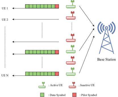
Figure 1: Uplink scenario of an mMTC cell with single BS and $N$ synchronized UEs

Consider a cell of an mMTC system consisting of a base station (BS) and $N$ user equipments (UE). The system allocates $M<N$ resources for creating a grant-free NOMA network consisting of the above UEs. The number $N$ can be rather large. Nevertheless, only a small fraction of these $N$ UEs initiate sporadic transmission at any given point of time [7]. This fraction is commonly referred as the activation probability $p_{a}$ in literature. In this system each UE is allocated its own spreading sequence. The spreading sequence allocated to user $n$ is given by an $M$ dimensional complex valued vector $\boldsymbol{\phi}_{n}$.

During a random access opportunity, a UE transmits over $J$ time-slots. At the $j$ th time-slot, the $n$ th user spreads its complex scalar valued data symbol $\beta_{n,j}$ over $M$ orthogonal resources using its spreading sequence $\boldsymbol{\phi}_{n}$. It forms the vector $\boldsymbol{\phi}_{n}\beta_{n,j}$. Subsequently, it transmits the $m$ th component of $\boldsymbol{\phi}_{n}\beta_{n,j}$ via the $m$ th orthogonal resource at $j$ th time-slot. Note that $\beta_{n,j}=0$ for all $j$ if user $n$ is inactive.

The signal received by the BS consists of all transmissions. Using the signal received during the random access opportunity, the BS forms the complex-valued vectors $\{{\bf y}_{j}\}_{j=1}^{J}$. Each ${\bf y}_{j}$ is an $M$ dimensional vector formed by arranging the data received in $M$ individual resources during the $j$ th time-slot. The vector ${\bf y}_{j}$ can be written as

$${\bf y}_{j} =\sum_{n\in\mathcal{N}}\boldsymbol{\phi}_{n}\beta_{n,j}h_{n}+{\bf w}_{j},\ \ j=1,2,\ldots,J.$$ (1)

where, $\mathcal{N}$ denotes the set of active users during the random access opportunity. In (1) we assume flat Rayleigh fading channels in uplink, and all $M$ orthogonal channels fall within coherent bandwidth [15]. Therefore, user $n$ experiences the same complex, scalar valued channel gain $h_{n}$ in all resources.

In (1), ${\bf w}_{j}$ denotes the complex vector valued measurement noise. We assume that the random vectors ${\bf w}_{1},{\bf w}_{2},\ldots,{\bf w}_{J}$ are mutually independent, and identically distributed with a mean zero, and covariance matrix $\sigma^{2}I$, where $\sigma$ is unknown.

For any active user $n$ it is assumed that $\beta_{n,1}=1$. This is the first data symbol that acts as the pilot. Subsequently, for all $j>1$, we assume $|\beta_{n,j}|=1$ provided that user $n$ is active. This is true when the data symbols are drawn from some PSK constellation. This assumption on $\beta_{n,j}$ are not necessary for the code detection step of our algorithm. We use this assumption in developing a joint channel and data estimation technique.

In the sequel we use $a_{n}$ to denote the index of $n$ th active user. Therefore,

$$\mathcal{N}=\{a_{1},a_{2},\ldots,a_{|\mathcal{N}|}\}.$$ (2)

Note that $|\mathcal{N}|$ denotes the cardinality of the set $\mathcal{N}$. Combining all received vectors over $J$ time-slots, we get the data matrix

$${\bf Y}=[{\bf y}_{1}\ {\bf y}_{2}\ \cdots\ {\bf y}_{J}].$$

Using (1) and (2) we can write ${\bf Y}$ as

$${\bf Y}=\Phi\Upsilon+{\bf W},$$ (3)

where ${\bf W}=[\ {\bf w}_{1}\ {\bf w}_{2}\ \cdots\ {\bf w}_{J}\ ]$,

$$\Phi=[\ \boldsymbol{\phi}_{a_{1}},\ \boldsymbol{\phi}_{a_{2}},\ \ \cdots\ \ ,\boldsymbol{\phi}_{a_{|\mathcal{N}|}}\ ],$$ (4)

and $\Upsilon$ is a $|\mathcal{N}|\times J$ matrix such that

$$\Upsilon_{n,j}=h_{a_{n}}\beta_{a_{n},j}.$$ (5)

III System Model with Sinusoidal Sequences

In the sequel, we work with sinusoidal spreading sequences. The $m$ th component of the spreading sequence $\boldsymbol{\phi}_{n}$ employed by user $n$ is given by

$$\boldsymbol{\phi}_{n}(m)=\gamma\exp(\mathrm{i}2\pi mn/N)\ \ m\in\{0,1,\cdots M-1\}.$$ (6)

Since $|\beta_{n,j}|=1$ for all $n$ and $j$, it follows that all UEs use the same transmit power proportional to $\gamma^{2}$.

III-A Signal model for sinusoidal spreading sequences

Note that the angular frequency of the sinusoidal spreading sequence employed by user $n$ is given by

$$\omega_{n}=2\pi n/N,\ n=0,1,\cdots,N-1.$$ (7)

With this, and (6), we can write the received signal at $m$ th resource of the $j$ th frame as

$${\bf y}_{j}(m)=\sum_{n\in\mathcal{N}}\exp(\mathrm{i}\omega_{n}m)x_{n,j}+{\bf w}_{j}(m),$$ (8)

$m\in\{0,1,\cdots M-1\}$ and $j\in\{0,1,\cdots J-1\}$, where $\mathcal{N}$ denotes the set of all active user indices, and we write

$$x_{n,j}=\gamma h_{n}\beta_{n,j}$$ (9)

for brevity.

Let us fix an integer $l$ of our choice. Then from (8) it follows for any $m\in\{0,1,\cdots M-l\}$ and $j\in\{0,1,\cdots J-1\}$ that

$${\bf s}_{m,j} :=[\ {\bf y}_{j}(m)\ {\bf y}_{j}(m+1)\ \cdots\ {\bf y}_{j}(m+l-1)\ ]^{\intercal}$$

$$=\sum_{n\in\mathcal{N}}\boldsymbol{\theta}_{n}x_{n,j}\exp(\mathrm{i}\omega_{n}m)+{\bf w}_{j}(m:m+l-1).$$ (10)

In above ${\bf w}_{j}(m:m+l-1)$ denotes the $l$ dimensional vector made up of the $m$ th through to the $m+l-1$ th components of ${\bf w}_{j}$, and in addition, we define

$$\boldsymbol{\theta}_{n}=[\ 1\ \exp(\mathrm{i}\omega_{n})\ \cdots\ \exp\{\mathrm{i}(l-1)\omega_{n}\}\ ]^{\intercal}.$$ (11)

From (10) it is readily verified that

$${\bf S}_{j}:=[\ {\bf s}_{0,j}\ {\bf s}_{1,j}\ \cdots\ {\bf s}_{M-l,j}\ ]=\sum_{n\in\mathcal{N}}\boldsymbol{\theta}_{n}\boldsymbol{\chi}^{\intercal}_{n,j}+{\bf W}_{j},$$ (12)

where

$$\boldsymbol{\chi}_{n,j} :=x_{n,j}[\ 1\ \exp(\mathrm{i}\omega_{n})\ \cdots\ \exp\{\mathrm{i}(M-l)\omega_{n}\}\ ]^{\intercal},$$ (13)

$${\bf W}_{j} =\left[\begin{array}[]{cccc}{\bf w}_{j}(0)&{\bf w}_{j}(1)&\cdots&{\bf w}_{j}(M-l)\\ {\bf w}_{j}(1)&{\bf w}_{j}(2)&\cdots&{\bf w}_{j}(M-l+1)\\ {\bf w}_{j}(l-1)&{\bf w}_{j}(l)&\cdots&{\bf w}_{j}(M-1)\end{array}\right].$$ (17)

Define the $l\times l$ anti-diagonal matrix ${\bf K}$ such that

$${\bf K}=\left[\begin{array}[]{cccc}0&\cdots&0&1\\ \vdots&\iddots&1&0\\ 0&\iddots&\iddots&\vdots\\ 1&0&\cdots&0\end{array}\right].$$

For any column vector $\boldsymbol{a}$ the product ${\bf K}\boldsymbol{a}$ is same as $\boldsymbol{a}$ flipped upside down. In particular, if $\mathrm{conj}(\boldsymbol{a})$ denotes the complex conjugate of $\boldsymbol{a}$, then it is readily verified that

$${\bf K}\ \mathrm{conj}(\boldsymbol{\theta}_{n})=\boldsymbol{\theta}_{n}\exp\{-\mathrm{i}\omega_{n}(l-1)\}.$$

Therefore, (12) yields that

$${\bf K}\ \mathrm{conj}({\bf S}_{j})=\sum_{n\in\mathcal{N}}\boldsymbol{\theta}_{n}\boldsymbol{\chi}^{*}_{n,j}\exp\{-\mathrm{i}\omega_{n}(l-1)\}+{\bf K}\ \mathrm{conj}({\bf W}_{j}),$$

where $\boldsymbol{\chi}^{*}_{n,j}$ denotes the conjugate transpose of $\boldsymbol{\chi}_{n,j}$. By combining the last equality with (10) it follows that

$$\bar{{\bf S}}_{j}:=[\ {\bf S}_{j}\ \ {\bf K}\ \mathrm{conj}({\bf S}_{j})\ ]=\sum_{n\in\mathcal{N}}\boldsymbol{\theta}_{n}\bar{\boldsymbol{\chi}}^{*}_{n,j}+\bar{{\bf W}}_{j},$$ (18)

where

$$\begin{split}\bar{\boldsymbol{\chi}}_{n,j}&=[\ \boldsymbol{\chi}_{n,j}^{\intercal}\ \ \boldsymbol{\chi}^{*}_{n,j}\mathrm{e}^{-\mathrm{i}\omega_{n}(l-1)}\ ]^{*},\\ \bar{{\bf W}}_{j}&=[\ {\bf W}_{j}\ \ \ {\bf K}\ \mathrm{conj}({\bf W}_{j})\ ].\end{split}$$ (19)

Now considering (18) for $j=0,1,\ldots,J-1$, we get

$$\overline{{\bf S}}=[\ \bar{{\bf S}}_{0}\ \bar{{\bf S}}_{1}\ \cdots\ \bar{{\bf S}}_{J-1}\ ]=\sum_{n\in\mathcal{N}}\boldsymbol{\theta}_{n}\boldsymbol{\psi}^{*}_{n}+\overline{{\bf W}},$$ (20)

where

$$\begin{split}\boldsymbol{\psi}_{n}&=[\ \bar{\boldsymbol{\chi}}_{n,0}^{*}\ \ \bar{\boldsymbol{\chi}}^{*}_{n,1}\ \ \cdots\ \ \bar{\boldsymbol{\chi}}_{n,J-1}^{*}\ ]^{*},\\ \overline{{\bf W}}&=[\ \bar{{\bf W}}_{0}\ \ \bar{{\bf W}}_{1}\ \ \cdots\ \ \bar{{\bf W}}_{J-1}\ ].\end{split}$$ (21)

Given the signal received at the BS, and a suitable integer $l$ of our choice, we can readily form the data matrix $\overline{{\bf S}}$ via the first equalities in the equations (10), (12), (18) and (20). The matrix $\overline{{\bf S}}$ has $l$ rows and $2J(M-l+1)$ columns. The rank of it’s noise-free part, which is given as

$$\overline{{\bf S}}-\overline{{\bf W}}=\sum_{n\in\mathcal{N}}\boldsymbol{\theta}_{n}\boldsymbol{\psi}^{*}_{n},$$

can not be more than $|\mathcal{N}|$. Therefore, if we take a large enough $l$ so that $l$ is always larger than $|\mathcal{N}|$, then $\overline{{\bf S}}-\overline{{\bf W}}$ will be of rank $|\mathcal{N}|$. This property can be exploited by subspace algorithms [24] . These algorithms work by obtaining a low rank approximation of $\overline{{\bf S}}$ via its singular value decomposition. The details are discussed below.

IV Fast Subspace Based AUD

IV-A Estimation of Number of Active Users

Note that the column-space of of the noise-free data $\overline{{\bf S}}-\overline{{\bf W}}$ is spanned by the vectors $\boldsymbol{\theta}_{n},n\in\mathcal{N}$. Subspace algorithm estimates this subspace via the eigen decomposition of $\overline{{\bf S}}$ [24]. Subspace algorithms like MUSIC [17] or ESPRIT [18] require the knowledge of number of signals to be specified as a priori. This is also the case for most of the CS-MUD algorithms where this information is decoded as prior sparsity level [11]. However, there exist sparsity-blind greedy algorithms which assume the availability of perfect channel knowledge or noise statistics at BS [12, 25]. In Bayesian approaches, this information is supplied to the algorithms as user activation probability $p_{a}$ which is derived from empirical studies [15]. In this work, however, we assume none of these information are available to BS. Specifically, we employ an information-criteria aided model order selection technique to find the number of active users in a random access opportunity.

In the sequel $\hat{\mathcal{N}}$ denotes the set of estimated active user indices. Hence, $|\hat{\mathcal{N}}|$ denotes the number of estimated active users. Given the data matrix $\overline{{\bf S}}$ an information-criterion aided technique estimates $|\hat{\mathcal{N}}|$ as

$$|\hat{\mathcal{N}}|=\arg\min_{k}\ -\log f(\overline{{\bf S}},k)+\mathcal{W}_{k}$$ (22)

where $\mathcal{W}_{k}$ is a bias correction term that depends on the information criterion being used, and as shown in [26], the log-likelihood function in (22) is given by

$$\log f(\overline{{\bf S}},k)=(l-k)\mathcal{\mathcal{P}}\ \ln\left\{\frac{\displaystyle\prod_{i=k+1}^{l}(\varsigma_{i}^{2}/\mathcal{\mathcal{P}})^{\frac{1}{l-k}}}{\frac{1}{l-k}\displaystyle\sum_{i=k+1}^{l}\varsigma_{i}^{2}/\mathcal{\mathcal{P}}}\right\},$$ (23)

where $\mathcal{P}$ is the number of columns in $\overline{{\bf S}}$ i.e:

$$\mathcal{P}=2J(M-l+1),$$

and $\{\varsigma\}_{i=1}^{l}$ denote the $l$ non-zero singular values of the $l\times\mathcal{P}$ matrix $\overline{{\bf S}}$. In particular, we assume without any loss of generality that

$$\varsigma_{1}>\varsigma_{2}>\cdots>\varsigma_{l}.$$

Several different information criteria can be used to determine how $\mathcal{W}_{k}$ depends on $k$ [26, 21, 27, 28]. For example one can use the classical information criterion by Alaike [29], for which $\mathcal{W}_{k}=k(2l-k)$ [26]. However, it is wellknown that AIC leads to overestimation of $|\hat{\mathcal{N}}|$. From that perspective it is better to use the Bayesian Information Criteria (BIC) proposed in [20] for which

$$\mathcal{W}_{k}=\frac{1}{2}k(2l-k)\log\mathcal{P}.$$ (24)

Using the singular value decomposition of $\overline{{\bf S}}$ one can readily calculate the cost in (22) via (23) and (24) for different values of $k$. Therefore it is rather straightforward to estimate $|\hat{\mathcal{N}}|$.

IV-B Finding the Active User Indices

Among many suitable candidates of subspace algorithms such as MUSIC, root-MUSIC, in this work, we employ ESPRIT [18]. ESPRIT has been recommended as a first choice in frequency estimation problem in [24]. In particular, the data model (20) leads to ESPRIT with forward-backward averaging which has been shown to have substantially improved statistical performance figures [30]. This process yields the set of angular frequencies of sinusoidal spreading sequences $\{\hat{\omega}_{n}\}_{i=1}^{|\hat{\mathcal{N}}|}$ used by the active users. The main steps of the ESPRIT algorithm is as follows:

1. Construct $\Theta=[{\bf u}_{1}\ {\bf u}_{2}\ \dots\ {\bf u}_{|\hat{\mathcal{N}}|}]$, where ${\bf u}_{k}$ denotes the unit norm left singular vector of $\overline{{\bf S}}$ associated with its $k$ th largest singular value $\varsigma_{k}$.

2. Solve the equation

   $$\Theta(1:l-1,:)\ {\bf Q}=\Theta(2:l,:)$$

   for ${\bf Q}$ in least squares sense.

3. Compute eigenvalues $\{\nu_{n}\}_{i=1}^{|\hat{\mathcal{N}}|}$ of ${\bf Q}$.

4. Estimate the frequencies $\{\hat{\omega}_{n}\}_{i=1}^{|\hat{\mathcal{N}}|}$ as

   $$\hat{\omega}_{n}=\arg(\nu_{n}),\hskip 17.07182ptn=1,2,\ldots,|\hat{\mathcal{N}}|.$$

We use $\hat{a}_{n}$ to denote the $n$ th estimated active user index. In other words,

$$\hat{\mathcal{N}}=\{\hat{a}_{1},\hat{a}_{2},\ldots,\hat{a}_{|\hat{\mathcal{N}}|}\}.$$

To find $\hat{a}_{n}$, we use the definition of $\omega_{n}$ given in (7), to get

$$\hat{a}_{n}=\mathrm{round}\left(\frac{N\hat{\omega}_{n}}{2\pi}\right).$$

IV-C Maximum Likelihood Estimate of Active User Indices

If the noise variance in (20) is large then it one may optionally improve the accuracy of the ESPRIT estimates by applying the Gaussian maximum-likelihood method [23], which requires us to solve,

$$\underset{\Upsilon,\ \{\hat{\omega}_{n}\}_{n=1}^{|\hat{\mathcal{N}}|}}{\mathrm{minimize}}\ \|{\bf Y}-\Phi\Upsilon\|_{F}^{2},$$ (25)

see (3) and (6) to recall how $\Phi$ depends on $\{\hat{\omega}_{n}\}_{n=1}^{|\hat{\mathcal{N}}|}$. Noting that, (25) is quadratic in $\Upsilon\in\mathbb{C}^{|\mathcal{N}|\times J}$, we can use linear least square to minimize (25) with respect to $\Upsilon$ which yields

$$\arg\min_{\Upsilon}\|{\bf Y}-\Phi\Upsilon\|_{F}^{2}=(\Phi^{*}\Phi)^{-1}\Phi^{*}{\bf Y},$$ (26)

and consequently it follows that

$$\min_{\Upsilon}\|{\bf Y}-\Phi\Upsilon\|_{F}^{2}=||{\bf Y}^{*}\{{\bf I}-\Phi(\Phi^{*}\Phi)^{-1}\Phi^{*}\}{\bf Y}||_{F}^{2}.$$ (27)

From (4) note that $\Phi$ depends on the spreading sequences, which by (6) depends on the frequencies. Hence the reduced cost function in the right hand side of (26) depends on the frequencies. Hence the maximum likelihood estimate of the frequencies can be obtained by solving

$$\underset{\{\hat{\omega}_{n}\}_{n=1}^{|\hat{\mathcal{N}}|}}{\mathrm{minimize}}\ ||{\bf Y}^{*}\{{\bf I}-\Phi(\Phi^{*}\Phi)^{-1}\Phi^{*}\}{\bf Y}||_{F}^{2}.$$ (28)

The cost function in (28) is non-convex in $\hat{\omega}_{n},\ n\in\hat{\mathcal{N}}$. Nevertheless, (28) turns out to be a variable projection problem, [22] for which well known algorithms exist [22]. These algorithms are wellknown to converge very quickly when initialized at a point near the global optimum. For our problem we can use the ESPRIT estimates $\{\hat{\omega}_{n}\}_{n\in\hat{\mathcal{N}}}$ to initialize the variable projection algorithm. As will be reiterated in later section, the algorithm converges within $2\sim 3$ iterations when $p_{a}<0.25$. Upon convergence, we update the frequency estimates $\{\hat{\omega}_{n}\}_{n\in\hat{\mathcal{N}}}$ by the corresponding ML estimates and find the set of active user indices $\hat{\mathcal{N}}$ as mentioned in previous section.

V Channel Estimation and Data Detection

In this section, we delineate the methods of channel estimation and data detection. In contrast with existing works where only signal received in the pilot frame is used, we use the entire received signal matrix ${\bf Y}\in\mathbb{C}^{M\times J}$ for channel estimation. The role of pilot symbol is to estimate the phase angle of estimated complex channel gains $\{h_{i}\}_{i=1}^{|\hat{\mathcal{N}}|}$ accurately as will be shown in following section.

V-A Channel Estimation

Using the detected active user indices we construct the $M\times|\hat{\mathcal{N}}|$ matrix $\hat{\Phi}$ such that

$$[\hat{\Phi}]_{m,n}=\gamma\exp(\mathrm{i}2\pi m\hat{a}_{n}/N).$$ (29)

Using $\hat{\Phi}$ we can find an estimate of $\Upsilon$, see (26),

$$\hat{\Upsilon}=(\hat{\Phi}^{*}\hat{\Phi})^{-1}\hat{\Phi}^{*}{\bf Y}.$$ (30)

Note that $\tilde{\Upsilon}\in\mathbb{C}^{\hat{|\mathcal{N}|}\times J}$.

In the system considered herein uses a a $L$-PSK constellation. Define the set

$$\mathcal{A}=\{0,1,2,\cdots\ L-1\}.$$ (31)

Hence $\beta_{a_{n},j}$ must be of the form

$$\beta_{a_{n},j}=\exp(\mathrm{i}2\pi q_{a_{n},j}/L)$$ (32)

where each $q_{a_{n},j}\in\mathcal{A}$. The data detection problem requires us to estimate $q_{\hat{a}_{n},j}$ for all $\hat{a}_{n}\in\hat{\mathcal{N}}$ and $j=2,3,\ldots,J$. We remind the readers that the pilot symbols equal to unity, i.e.

$$\beta_{\hat{a}_{n},1}=1,\hskip 17.07182pt\Leftrightarrow\hskip 17.07182ptq_{\hat{a}_{n},1}=0$$ (33)

for all $\hat{a}_{n}\in\hat{\mathcal{N}}$.

Now recalling (5) and using (32) we can write

$$\Upsilon_{n,j} =h_{a_{n}}\beta_{a_{n},j}=|h_{a_{n}}|\exp\left(\mathrm{i}\left\{\zeta_{a_{n}}+\frac{2\pi}{L}q_{a_{n},j}\right\}\right)$$ (34)

where $\zeta_{a_{n}}$ is the phase angle of channel gain i.e: $h_{a_{n}}=|h_{a_{n}}|\exp(\mathrm{i}\zeta_{a_{n}})$. Taking natural logarithm at both sides of (34) we get

$$\ln{(\Upsilon_{n,j})}=\ln(|h_{a_{n}}|)+\mathrm{i}\left(\zeta_{a_{n}}+\frac{2\pi}{L}q_{a_{n},j}\right),$$ (35)

so that

$$\mathrm{Re}\{\ln{(\Upsilon_{n,j})}\}=\ln(|h_{a_{n}}|),$$ (36)

$$L\mathrm{Im}\{\ln{(\Upsilon_{n,j})}\}=L\zeta_{a_{n}}+2\pi q_{a_{n},j}.$$ (37)

Since each $q_{a_{n},j}\in\{0,1,2,\ldots,L-1\}$, it follows that

$$\mathrm{mod}(L\mathrm{Im}\{\ln{(\Upsilon_{n,j})}\}\ ,\ 2\pi)=\mathrm{mod}(L\zeta_{a_{n}}\ ,\ 2\pi).$$ (38)

Next we replace $\Upsilon$ by its estimate $\hat{\Upsilon}$ in (30). The estimate $\hat{\Upsilon}$ will not be error-free. We propose to reduce the effect of the estimation error by averaging. Using (36) we estimate $|h_{\hat{a}_{n}}|$ for each $\hat{a}_{n}\in\hat{\mathcal{N}}$ as

$$|\hat{h}_{\hat{a}_{n}}|=\frac{1}{J}\sum_{j=1}^{J}\mathrm{Re}\{\ln{(\hat{\Upsilon}_{n,j})}\}.$$ (39)

Similarly, using (38) we estimate $\mathrm{mod}(L\zeta_{\hat{a}_{n}}\ ,\ 2\pi)$ by

$$\bar{\zeta}_{\hat{a}_{n}}=\frac{1}{J}\sum_{j=1}^{J}\mathrm{mod}(L\mathrm{Im}\{\ln{(\Upsilon_{n,j})}\},2\pi).$$ (40)

Since $\bar{\zeta}_{\hat{a}_{n}}$ is an estimate of $\mathrm{mod}(L\zeta_{\hat{a}_{n}},2\pi)$ , we have $L$ possible candidates which can be an estimate of $\zeta_{\hat{a}_{n}}$. These are the elements of the set

$$\mathcal{J}=\left\{\bar{\zeta}_{\hat{a}_{n}}+\frac{2\pi k}{L}\ :\ k\in\mathcal{A}\right\}.$$

To identify the correct candidate from the above set we make use of (33) and (34), which yield

$$\Upsilon_{n,1} =h_{a_{n}}=|h_{a_{n}}|\exp(\mathrm{i}\zeta_{a_{n}}).$$ (41)

Equation (41) reveals that $\hat{\Upsilon}_{n,1}$ is, in fact, an estimate of $h_{\hat{a}_{n}}$. But this estimate being based on only one element of $\hat{\Upsilon}$, is more noisy than our proposed estimate based on the averaged statistics in (39) in (40). Nevertheless, we can use $\hat{\Upsilon}_{n,1}$ to identify the correct candidate from $\mathcal{J}$. In particular we estimate $\zeta_{\hat{a}_{n}}$ by

$$\hat{\zeta}_{\hat{a}_{n}}=\arg\min_{\zeta\in\mathcal{J}}\ \left|\mathrm{e}^{\mathrm{i}\zeta}-\frac{\hat{\Upsilon}_{n,1}}{|\hat{\Upsilon}_{n,1}|}\right|.$$ (42)

V-B Data Detection

Our data detection method is based on (34), which yields

$$\frac{\Upsilon_{n,j}}{|\Upsilon_{n,j}|}\mathrm{e}^{-\mathrm{i}\zeta_{a_{n}}}=\exp(\mathrm{i}2\pi q_{a_{n},j}/L).$$ (43)

Motivated by (43), and using the estimates $\hat{\Upsilon}_{n,j}$ and $\hat{\zeta}_{\hat{a}_{n}}$ (obtained in (42)) we propose to estimate $q_{\hat{a}_{n},j}$ as

$$\hat{q}_{\hat{a}_{n},j}=\arg\min_{q\in\mathcal{A}}\ \left|\frac{\hat{\Upsilon}_{n,j}}{|\hat{\Upsilon}_{n,j}|}\exp(-\mathrm{i}\hat{\zeta}_{\hat{a}_{n}})-\exp(\mathrm{i}2\pi q/L)\right|.$$ (44)

V-C Condition for Reliable Data Detection

An UE located near the cell boundary experiences high path-loss, and have low signal to noise ratio (SIR). It is wellknown that the detection-estimation algorithms have difficulties in detecting such users experiencing deep fading. Nevertheless, in our simulation study we have observed that the proposed user detection method is often capable of detecting such low-SNR UEs, but the data detection method outlined in the previous sub-section may not produce accurate results. It is of significant interest for the system designer to be able to detect such users. Because this allows the BS to send an ARQ like signal to this users, and those users can use a higher transmit power in their next random access attempt. Such ARQ like mechanisms can greatly improve the overall network performance. In this section we briefly discuss how such low SNR users could be identified within the framework proposed herein.

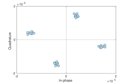
(a)

(b)

Figure 2: (a) Received symbols of reliable UE (b) Received symbols of a non-reliable UE

We use Figure 2 to examine why data detection becomes difficult for a low SNR user. In Figure 2a we show the typical scatter plot of $\hat{\Upsilon}_{n,j}$ for a fixed $n$ as $j$ varies from $1$ to $J$. In this example $L=4$. Recall from (34) that $|\Upsilon_{n,j}|=|h_{a_{n}}|$ for all $j$, while the phase of $\Upsilon_{n,j}$ can have only $4$ different values. In particular, a scatter plot of $\Upsilon_{n,j}$ should look like the $4$-PSK constellation rotated by $\zeta_{a_{n}}$. The plot in Figure 2a is consistent with this expectation with exception that we see the points 4 distinct clusters instead of exactly 4 points. This is not a surprise as the deviation from the cluster centers are caused by the estimation errors in $\hat{\Upsilon}_{n,j}$ contributed by the measurement noise in the observed data. In this case the spread of the points caused by the measurement noise is small compared to the average value of $|\hat{\Upsilon}_{n,j}|$ which determine the radius of the circle on which the cluster center lie.

The situation becomes worse for another user with a scatter plot shown Figure 2b. This user is experiencing much higher path-loss, and thus has a significantly smaller averaged $|\hat{\Upsilon}_{n,j}|$. This significantly shrinks the circle on which the cluster centers lie. Consequently, the inter-cluster separation is of the same order as the perturbation of the constellation points due to noise. At this stage the data detector may not be able to provide perfect data detection results.

The above example reveals that we can have perfect data detection only if the averaged $|\hat{\Upsilon}_{n,j}|$ is large compared to the perturbation due to noise. From (36) we note that $|\hat{h}_{\hat{a}_{n}}|$ is the average value of $|\hat{\Upsilon}_{n,j}|$. One simple way to estimate the spread caused by the noise would be calculate the corresponding standard deviation

$$\eta_{\hat{a}_{n}}:=\sqrt{\frac{1}{J}\sum_{j=1}^{J}\left(\mathrm{Re}\{\mathrm{ln}(\hat{\Upsilon}_{n,j})\}-|\hat{h}_{\hat{a}_{n}}|\right)^{2}.}$$ (45)

Now the distance between the neighboring cluster centers for the estimated active user index is $2|\hat{h}_{\hat{a}_{n}}|\sin(\pi/L)$. This distance must be more than twice the estimation error spread for reliable data detection. Assuming normal distributed estimation error, we take the spread to be $5\eta_{\hat{a}_{n}}$ with $99.9\%$ confidence. Hence to ensure $99.9\%$ confidence in data detection we need

$$2|\hat{h}_{\hat{a}_{n}}|\sin(\pi/L)>2\times 5\eta_{\hat{a}_{n}}\hskip 17.07182pt\Leftrightarrow$$

$$|\hat{h}_{\hat{a}_{n}}|/\eta_{\hat{a}_{n}}/>\lambda=5/\sin(\pi/L).$$ (46)

To increase the confidence level we need to increase $\lambda$. Note that $\lambda$ increases if either of $L$ or the noise power increases. In practice, one can implement a protocol where the BS proceeds with data detection if (46) holds. Otherwise, BS can notify the user to transmit the data once more with higher transmit power.

V-D Summary of fast subspace based AUD, CE and DD

In this section, we summarize the steps of the proposed algorithms. The input of the algorithm is the received signal matrix ${\bf Y}\in\mathbb{C}^{M\times J}$ as in (3). With these, we form the data matrix $\overline{{\bf S}}$ as in (20). Then the proposed method carries out following steps in sequel:

1. Computes singular value decomposition (SVD) of $\overline{{\bf S}}$

2. Estimates $|\hat{\mathcal{N}}|$ via (22). For that it must calculate the log-likelihood as in (23) and the bias correction term in (24) for each competing model order $k$.

3. Estimates angular frequencies $\{\hat{\omega}_{n}\}_{n=1}^{|\hat{\mathcal{N}}|}$ using a subspace algorithm. In the sequel we have used forward-backward ESPRIT outlined in Section IV-B. One may optionally use the ESPRIT estimates to initialize a variable projection algorithm (28), and find Gaussian ML estimates, which are more accurate.

4. Using the frequency estimates obtained in previous stage, it determines the set of estimated active user indices $\hat{\mathcal{N}}$, and find $\hat{\Upsilon}$, see (30).

5. For each $n=1,2,\ldots,\hat{\mathcal{N}}$

   • Finds $|\hat{h}_{\hat{a}_{n}}|$ in (39), $\hat{\zeta}_{\hat{a}_{n}}$ in (42), and $\eta_{\hat{a}_{n}}$ in (45).

   • If $\eta_{\hat{a}_{n}}/|\hat{h}_{\hat{a}_{n}}|>\lambda$ then carries out data detection for $j=2,3,\ldots,J$ as per (44). Otherwise requests the user to retransmit with higher transmit power.

VI Numerical simulation studies

VI-A Simulation Setup

We consider an mMTC scenario with $N=128$ UEs. These are randomly deployed within the cell of radius 200 m. An UE is at least 1m away from the BS. The variance $\tau_{n}$ (in dB) of $h_{n}$ is modeled using NLOS model in 3GPP (release 9):

$$\tau_{n}=-128.1-36.7\log_{10}(d_{n}),$$ (47)

where $d_{n}$ is the distance between $n$ th UE and BS in km. For receiver noise, the power spectral density is set at $-170$ dBm/Hz, and the transmission bandwidth is set at 1 MHz. A random access opportunity consists of $J=9$ frames, the first ($j=1$) of which is used to transmit pilot symbol. The pilot symbol $\beta_{n,1}=1$ for all active UE. The PSK constellations use $L=4$. This setup is identical to that used in [15].

The expectation-propagation (EP) approach proposed in [15] is used as the benchmark for performance comparison. This choice is well justified. In [15] EP has been shown outperform all major existing methods by a comprehensive margin.

As performance metrics, we consider Missed Detection Rate (MDR), Net Symbol Error Rate (NSER) and Root Mean Squared Error (RMSE) of CE. MDR refers to the rate of UEs failing to get recognized by candidate algorithms during AUD. On the other hand, NSER is the symbol error rate experienced by active UEs. These performance metrics are evaluated as a function of sequence length $M$, user activation probability $p_{a}$ and transmit power. Each point in the plots shown in the sequel are based on 10000 independent Monte-Carlo simulations. Performance of EP algorithm is evaluated using both random and sinusoidal spreading codes which are denoted as EP with RC and EP with SC, respectively. The performance of ESPRIT algorithm alone is denoted as ESPRIT whereas the performance of ESPRIT initialized variable projection based estimation is denoted as ESP-VPN. Unless specified otherwise, $M=64$, $p_{a}=0.1$, and all UEs transmit with $20$ dBm. For ESPRIT we need to choose the integer $l$ in (10). In our simulations we vary $l$ depending on $M$ as follows

$M$	32	48	64	80	96	112
$l$	20	40	50	60	78	90

These values are chosen to optimize the estimation performance.

VI-B Simulation Results

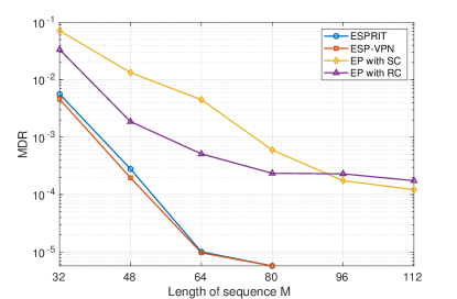
(a)

(b)

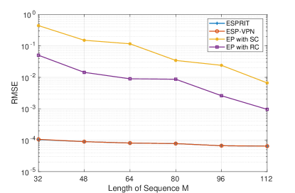
(c)

Figure 3: (a) MDR (b) NSER (c) RMSE of different methods as functions of $M$.

Figure 3 plots the MDR, NSER and RMSE performance of different algorithms where $M$ is varied from $32$ to $112$. In this study we fix transmit power to $20$ dBm and $p_{a}=0.1$. As can be seen in Figure 3, the proposed algorithm achieves significant performance improvement in all performance metrics over the EP algorithm. ESP-VPN offers slight performance improvement for $M<64$. Unlike EP, channel estimation accuracy of the proposed method does not vary much with $M$ in Figure 3b. Note that the performance of EP often deteriorates with sinusoidal sequences.

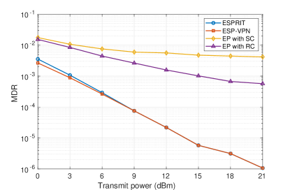
(a)

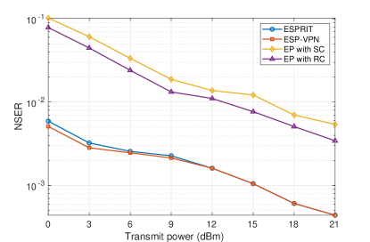
(b)

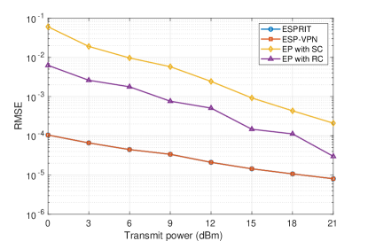
(c)

Figure 4: (a) MDR (b) NSER (c) RMSE as functions of transmit power.

Figure 4 plots the MDR, NSER and RMSE of different methods as functions of the transmit power, while we fix $M=64$, $p_{a}=0.1$. As before, the proposed algorithm outperforms EP in all performance criteria. For transmit power below $6$ dBm ESP-VPN provides some performance improvement over ESPRIT in terms of MDR and NSER. EP with random sequence continues to perform better.

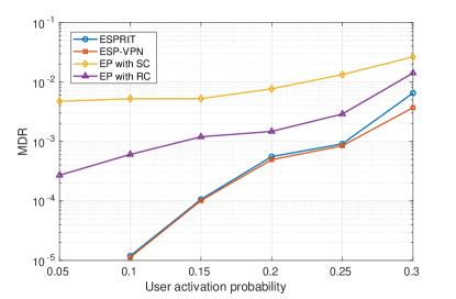
(a)

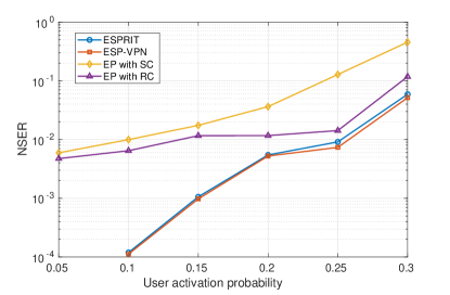
(b)

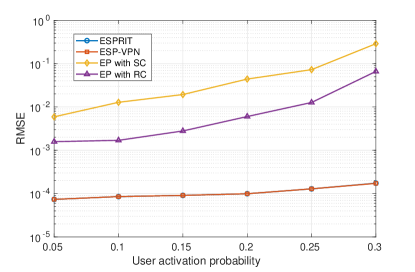
(c)

Figure 5: (a) MDR (b) NSER (c) RMSE as functions of $p_{a}$.

Figure 5 plots the performance metrics as functions of user activation probability $p_{a}$, while the transmit power is 20 dBm and $M=64$. As expected, all methods suffer from performance degradation as $p_{a}$ increases causing higher interference among UE. For the proposed method, an increased number of active UEs increases probability of having active UEs with closely spaced angular frequencies. This limits the performance of ESPRIT. In this case, ESP-VPN can offer slight performance improvements for $p_{a}\geq 0.2$, see Figures 5a and 5b.

(a)

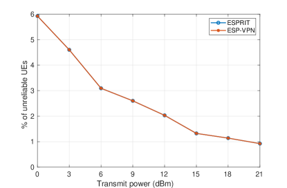
(b)

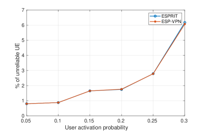
(c)

Figure 6: % of unreliable UEs as functions of (a) $M$, (b) transmit power, and (c) $p_{a}$.

Figure 6 shows the influence of $M,p_{a},$ and transmit power on the percentage of UEs whose data cannot be detected reliably as per (46). From Figure 6(b), where $M=64$, there are only 6% of such ‘unreliable UEs’ even at $0$ dBm transmit power. In addition, ESP-VPN offers some small improvements if $p_{a}$ is high.

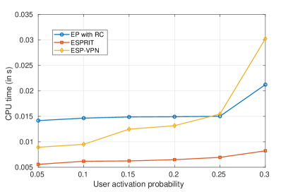
(a)

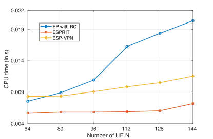
(b)

Figure 7: Average CPU time taken by different methods as functions of (a) $p_{a}$ (b) $N$.

In Figure 7 we plot the average CPU time required by different methods for active user identification, estimation of channel gains, and data decoding for $M=64$ and $20$ dBm transmit power. Here EP is run for 3 iterations (as per [15], the additional iterations do not improve EP’s performance). As suggested in [15], Woodbury Identity and Cholesky decomposition is used for certain matrix inversion within the EP algorithm for reducing computational cost. All of the algorithms are implemented in MATLAB on an Intel Core i7 2600, eight-core computer clocked at 3.40 GHz with 16.0 GB RAM. Figure 7 demonstrates the lower computational requirement of proposed methods. Proposed methods (both ESPRIT and ESP-VPN) offer faster estimation under varying user activation probability $p_{a}$, although at $p_{a}\geq 0.25$, ESP-VPN shows higher complexity than EP with random sequences. This is because at high $p_{a}$, ESP-VPN in (28) requires higher number of iterations ($3\sim 4$). Note that, $p_{a}\geq 0.25$ is not quite practical as per [7], where it has been concluded that $p_{a}\leq 0.1$ even at peak load. In fig. 7(b), we fix $p_{a}=0.1$, and plot computation time as function of the total number $N$ of UEs. The computation time of EP grows quickly with $N$ at a rate significantly faster than the proposed methods.

VII Conclusions

In this work, we have proposed to employ sinusoidal spreading sequences for UL grant-free mMTC system. This proposition effectively turns active user detection (AUD) problem into a frequency estimation problem which allows us to use non-iterative, low complexity, and accurate signal processing algorithms. In contrast with existing greedy and Bayesian algorithms in relevant literature, proposed method does not require any prior empirical assumption on channel/noise statistics and number of active users. Extensive numerical simulations show that, in most cases, proposed method outperforms state-of-art EP algorithm, which considered one of the best among the existing algorithms [15] in terms of several fundamental performance metrics, that too in expense of a lower computational cost. Based on the estimated knowledge of UE activity, we have proposed a new method of channel estimation. This method coherently processes all data frames to minimize the adverse effects of measurement noise on estimation-detection performance. This analysis also allows us to develop a threshold aided decision rule to identify the low SNR users, whose data symbols cannot be detected reliably.

References

- [1] H. Tullberg, P. Popovski, Z. Li, M. A. Uusitalo, A. Hoglund, O. Bulakci, M. Fallgren, and J. F. Monserrat, “The metis 5g system concept: Meeting the 5g requirements,” IEEE Communications Magazine, vol. 54, no. 12, pp. 132–139, 12 2016.
- [2] C. Bockelmann, N. Pratas, H. Nikopour, K. Au, T. Svensson, C. Stefanovic, P. Popovski, and A. Dekorsy, “Massive machine-type communications in 5g: physical and mac-layer solutions,” IEEE Communications Magazine, vol. 54, no. 9, pp. 59–65, 9 2016.
- [3] K. Au, L. Zhang, H. Nikopour, E. Yi, A. Bayesteh, U. Vilaipornsawai, J. Ma, and P. Zhu, “Uplink contention based scma for 5g radio access,” in 2014 IEEE Globecom Workshops (GC Wkshps), 12 2014, pp. 900–905.
- [4] Z. Ding, Y. Liu, J. Choi, Q. Sun, M. Elkashlan, C. I, and H. V. Poor, “Application of non-orthogonal multiple access in lte and 5g networks,” IEEE Communications Magazine, vol. 55, no. 2, pp. 185–191, 2 2017.
- [5] Y. Liu, Z. Qin, M. Elkashlan, Z. Ding, A. Nallanathan, and L. Hanzo, “Nonorthogonal multiple access for 5g and beyond,” Proceedings of the IEEE, vol. 105, no. 12, pp. 2347–2381, 12 2017.
- [6] M. Shirvanimoghaddam, M. Dohler, and S. J. Johnson, “Massive non-orthogonal multiple access for cellular iot: Potentials and limitations,” IEEE Communications Magazine, vol. 55, no. 9, pp. 55–61, 9 2017.
- [7] J. Hong, W. Choi, and B. D. Rao, “Sparsity controlled random multiple access with compressed sensing,” IEEE Transactions on Wireless Communications, vol. 14, no. 2, pp. 998–1010, 2 2015.
- [8] G. Swirszcz, N. Abe, and A. C. Lozano, “Grouped orthogonal matching pursuit for variable selection and prediction,” in Advances in Neural Information Processing Systems 22, Y. Bengio, D. Schuurmans, J. D. Lafferty, C. K. I. Williams, and A. Culotta, Eds. Curran Associates, Inc., 2009, pp. 1150–1158. [Online]. Available: http://papers.nips.cc/paper/3878-grouped-orthogonal-matching-pursuit-for-variable-selection-and-prediction.pdf
- [9] H. Schepker, C. Bockelmann, and A. Dekorsy, “Improving greedy compressive sensing based multi-user detection with iterative feedback,” 09 2013, pp. 1–5.
- [10] B. Wang, L. Dai, T. Mir, and Z. Wang, “Joint user activity and data detection based on structured compressive sensing for noma,” IEEE Communications Letters, vol. 20, no. 7, pp. 1473–1476, 7 2016.
- [11] J. Zhang, Y. Pan, and J. Xu, “Compressive sensing for joint user activity and data detection in grant-free noma,” IEEE Wireless Communications Letters, vol. 8, no. 3, pp. 857–860, 6 2019.
- [12] N. Y. Yu, “Multiuser activity and data detection via sparsity-blind greedy recovery for uplink grant-free noma,” IEEE Communications Letters, vol. 23, no. 11, pp. 2082–2085, 11 2019.
- [13] J. Fu, G. Wu, Y. Zhang, L. Deng, and S. Fang, “Active user identification based on asynchronous sparse bayesian learning with svm,” IEEE Access, vol. 7, pp. 108 116–108 124, 7 2019.
- [14] B. K. Jeong, B. Shim, and K. B. Lee, “Map-based active user and data detection for massive machine-type communications,” IEEE Transactions on Vehicular Technology, vol. 67, no. 9, pp. 8481–8494, 9 2018.
- [15] J. Ahn, B. Shim, and K. B. Lee, “Ep-based joint active user detection and channel estimation for massive machine-type communications,” IEEE Transactions on Communications, vol. 67, no. 7, pp. 5178–5189, 7 2019.
- [16] R. A. Horn and C. R. Johnson, Topics in Matrix Analysis. Cambridge University Press, 1991.
- [17] A. Barabell, “Improving the resolution performance of eigenstructure-based direction-finding algorithms,” in ICASSP ’83. IEEE International Conference on Acoustics, Speech, and Signal Processing, vol. 8, April 1983, pp. 336–339.
- [18] R. Roy and T. Kailath, “Esprit-estimation of signal parameters via rotational invariance techniques,” IEEE Transactions on Acoustics, Speech, and Signal Processing, vol. 37, no. 7, pp. 984–995, 07 1989.
- [19] C. M. HURVICH and C.-L. TSAI, “Regression and time series model selection in small samples,” Biometrika, vol. 76, no. 2, pp. 297–307, 06 1989. [Online]. Available: https://doi.org/10.1093/biomet/76.2.297
- [20] J. Rissanen, “Modeling by shortest data description,” Automatica, vol. 14, no. 5, pp. 465 – 471, 1978. [Online]. Available: http://www.sciencedirect.com/science/article/pii/0005109878900055
- [21] T.-J. Wu and A. Sepulveda, “The weighted average information criterion for order selection in time series and regression models,” Statistics and Probability Letters, vol. 39, no. 1, pp. 1 – 10, 1998. [Online]. Available: http://www.sciencedirect.com/science/article/pii/S0167715298000030
- [22] G. Golub and V. Pereyra, “Separable nonlinear least squares: the variable projection method and its applications,” Inverse Problems, vol. 19, pp. R1–R26(1), 01 2003.
- [23] P. Stoica, A. Jakobsson, and J. Li, “Cisoid parameter estimation in the colored noise case – asymptotic Cramér-Rao bound, maximum likelihood, and nonlinear least-squares,” IEEE Transactions on Signal Processing, vol. 45, pp. 2048–2059, 1997.
- [24] P. Stoica, R. L. Moses et al., “Spectral analysis of signals,” 2005.
- [25] J. Liu, G. Wu, S. Li, and O. Tirkkonen, “Blind detection of uplink grant-free scma with unknown user sparsity,” in 2017 IEEE International Conference on Communications (ICC), 5 2017, pp. 1–6.
- [26] M. Wax and T. Kailath, “Detection of signals by information theoretic criteria,” IEEE Transactions on Acoustics, Speech, and Signal Processing, vol. 33, no. 2, pp. 387–392, April 1985.
- [27] P. Chen, T. . Wu, and J. Yang, “A comparative study of model selection criteria for the number of signals,” IET Radar, Sonar Navigation, vol. 2, no. 3, pp. 180–188, June 2008.
- [28] H. Lütkepohl, “Comparison of criteria for estimating the order of a vector autoregressive process,” Journal of Time Series Analysis, vol. 6, no. 1, pp. 35–52, 1985. [Online]. Available: https://onlinelibrary.wiley.com/doi/abs/10.1111/j.1467-9892.1985.tb00396.x
- [29] H. Akaike, Information Theory and an Extension of the Maximum Likelihood Principle. New York, NY: Springer New York, 1998, pp. 199–213. [Online]. Available: https://doi.org/10.1007/978-1-4612-1694-0_15
- [30] R. Bachl, “The forward-backward averaging technique applied to tls-esprit processing,” IEEE Transactions on Signal Processing, vol. 43, no. 11, pp. 2691–2699, 11 1995.