Cosmology with the Einstein Telescope: No Slip Gravity Model and Redshift Specifications

Abstract

The Einstein Telescope and other third generation interferometric detectors of gravitational waves are projected to be operational post $2030$. The cosmological signatures of gravitational waves would undoubtedly shed light on any departure from the current gravitational framework. We here confront a specific modified gravity model, the No Slip Gravity model, with forecast observations of gravitational waves. We compare the predicted constraints on the dark energy equation of state parameters $w_{0}-w_{a}$, between the modified gravity model and that of Einstein gravity. We show that the No Slip Gravity model mimics closely the constraints from the standard gravitational theory, and that the cosmological constraints are very similar. The use of spectroscopic redshifts, especially in the low–redshift regime, lead to significant improvements in the inferred parameter constraints. We test how well such a prospective gravitational wave dataset would function at testing such models, and find that there are significant degeneracies between the modified gravity model parameters, and the cosmological parameters that determine the distance, due to the gravitational wave dimming effect of the modified theory.

I Introduction

In the current era of precision cosmology, observational probes of the expansion history and constituents of the Universe strongly rely on the so–called standard candles. Undoubtedly, Type Ia supernovae (SNe Ia) Riess:1998cb ; Perlmutter:1998np ; Kowalski:2008ez have extensively been used as standard candles, since their intrinsic luminosity is assumed to be known within a certain tolerance, and therefore these could be used to determine the luminosity distance. It is well–known that gravitational waves (GWs) emerging from binary systems also encode the absolute distance information Schutz:1986gp . The coalescence of compact binaries can be (and has been) used as standard sirens, since from the GW signal itself one would be able to measure the luminosity distance in an absolute way. These standard sirens are known to be self-calibrating, since these do not rely on a cosmic distance ladder. In order to get the redshift information of a GW event, and so place them on the luminosity distance–redshift $(D_{L}-z)$ relation, an accompanying electromagnetic signal is needed (see, for instance Oguri:2016dgk ; Ding:2018zrk ; Abbott:2019yzh ; Mukherjee:2020hyn ; Yu:2020agu , and references therein for other redshift measurement techniques in the case of dark standard sirens). Such a relation is clearly necessary for the reconstruction of the late–time cosmological expansion of the Universe, and has also been employed to constrain various cosmological parameters of modified theories of gravity.

The era of GW astronomy began with the detection of GW150914 Abbott:2016blz from the observation of a GW signal originating from the coalescence of a binary black hole (BBH), whereas the first detection of multi–messenger astronomy was reported with GW170817 TheLIGOScientific:2017qsa from a GW signal emitted by a binary neutron star (BNS) inspiral accompanied by electromagnetic detections. In contrast to standard candles, the determination of a GW event’s redshift is a non–trivial task, primarily because of the low resolution of the source’s sky localisation which typically is of $\sim\mathcal{O}(10)\,\mathrm{deg}^{2}$ accuracy Fairhurst:2009tc . On the other hand, the distance estimates from GWs are free from any external calibration requirements, which are necessary for the SNe Ia probe (the cosmic distance ladder).

The primary next generation, also known as third generation Evans:2016mbw , GW detectors will be the ground–based Einstein Telescope (ET) Punturo:2010zz and Cosmic Explorer (CE) 3 detectors (see, for instance, Jin:2020hmc for a comparison between the ET and CE), along with the space–based LISA/eLISA 2017arXiv170200786A ; AmaroSeoane:2012km and TianQin Luo:2015ght millihertz observatories. These GW detectors are expected to have a better sensitivity (by an order of magnitude in the strain amplitude of GWs) and a wider accessible frequency band with respect to currently available second generation detectors. The median redshift from the near future GW catalogue composed of the combined set of GW events from the planned GW detectors is envisaged to be at $z\sim 2$ Congedo:2018wfn . Clearly, such high redshift direct measurements of the luminosity distance would be clearly complementing the existing and upcoming SNe Ia measurements. In this analysis we will be focusing on the ET, although we believe that the consideration of the other third generation GW detectors would lead to interesting analyses.

The ET is expected to make independent estimates of the several cosmological parameters, including Zhang:2018byx ; Wang:2018lun ; Belgacem:2019tbw : the Hubble constant $(H_{0})$, matter content of the Universe $(\Omega_{m}^{0})$, spatial curvature $(\Omega_{k}^{0})$, and the dark energy equation of state parameters ($\{w_{0},\,w_{a}\}$, or alternative parameterisations). Indeed, it is anticipated that more than a thousand GW events need to be detected Cai:2016sby (see also Liao:2017ioi for the consideration of lensed GW events) in order to match the sensitivity of the Planck satellite Aghanim:2018eyx , and these envisaged to be confidently reported during the ET observation run. Although the ET would not be able to independently arrive to all the measurements of these parameters at once, the joint combination DAgostino:2019hvh ; Yang:2019bpr of the latter standard sirens data sets with the precise data sets inferred from the existing and forthcoming state–of–the–art electromagnetic probes, including measurements of the baryon acoustic oscillations (BAO) and of the cosmic microwave background (CMB), would significantly enhance our knowledge on the dynamics of the Universe. Furthermore, the opportunity of observing black holes back to a much earlier epoch of the Universe could allow us to observe the remnants of the first stars, and to explore the dark ages, during which proto-galaxies and large–scale structure emerged.

A number of recent works (see, for instance, 6 ; Yang:2019vni ; Zhang:2019ple ; Wolf:2019hun ; Yang:2020wby ; Bachega:2019fki ; Li:2019ajo , and references therein) have illustrated the strength of GW detections by their ability to constrain different dark energy models. Next generation GW detections also gives us the scope to perform tests on theories of modified gravity by confronting the modified propagation of GWs across cosmological distances. This is possible because of their higher source redshift and lesser calibration requirements. Modified theories of gravity are normally characterised by different evolution of scalar as well as tensor perturbations Nishizawa:2017nef . Consequently, any deviation from Einstein gravity could be parametrised in the propagation equation of GW by introducing new parameters related to (for example) the propagation speed of GWs, a friction term which dilutes the amplitude of GWs, graviton mass, or an energy source term. GW probes, particularly the upcoming detectors, have been shown (see, for instance, Sathyaprakash:2009xt ; Monitor:2017mdv ; Wang:2018lun ; Yang:2019vni ; Yang:2018bdf ; Zhang:2018byx ; Du:2018tia ; Lagos:2019kds ; Belgacem:2019zzu ; Zhang:2019ple ; Bachega:2019fki ; Yang:2019bpr ; Chen:2020lzc ; Sharma:2020btq ; Mastrogiovanni:2020gua and references therein) to be able to help shed light on deviations from Einstein gravity.

In this paper, we will present a comparative study of the cosmological dark energy parameter constraints we will be expecting from the upcoming GW observations between the existing standard dark energy models and modified gravity models. We also investigate how tests of the models may be confused by degeneracies between the modified theory predictions, and parameters that control the distance. In section II we discuss the proposed third generation GW detectors, while in section III we briefly review the theoretical framework of modified GW propagation. In section IV we illustrate the data and methodology which will be implemented in section V. We draw our final conclusions and prospective lines of research in section VI.

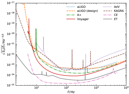
Figure 1: Sensitivity evolution of current and proposed GW interferometric detectors.

II Third Generation GW Detectors

The achieved sensitivity by the first generation of interferometric detectors (LIGO Abbott:2007kv , Virgo Acernese:2008zza , GEO 600 Grote:2008zz and TAMA Takahashi:2004rwa ) was mainly limited by shot noise, mirror thermal noise and seismic noise, while for the second generation GW detectors, such as Advanced LIGO (aLIGO) Harry:2010zz , Advanced Virgo (AdV) TheVirgo:2014hva , KAGRA Somiya:2011np ; Aso:2013eba , and LIGO-India Unnikrishnan:2013qwa additional fundamental noise sources will play a role towards the low–frequency end of the detection band. As expected, the latter noise sources will be more prominent in third generation GW detectors Hild:2010id ; Punturo:2010zzb ; Huttner:2016dzl , particularly due to the fact that the main aim of these detectors is to probe the low–frequency band; as low as a few Hz Hild:2009ns . This low–frequency range is one of the main driving forces of third generation GW detectors, since it encapsulates some rich information on the cosmological evolution of the Universe (see, for instance, Punturo:2010zza ; Sathyaprakash:2012jk ; Srivastava:2019fcb ; Maggiore:2019uih ; Zhang:2019ple ; Yang:2019vni ; Yang:2019bpr ; Bachega:2019fki ; Sathyaprakash:2009xt ; Chen:2020lzc ; Sharma:2020btq , and references therein).

$a_{t}$	$\tau$	$\mu$
0.5	1.5	0.1
	1.0	0.1
	1.0	0.2

Table 1: The three different combinations of adopted parameter values for $a_{t},\,\tau$ and $\mu$ 5 .

We should also remark that this young field of observational astrophysics is constantly being enhanced by technological improvements. Indeed, the current GW detectors are expected to be upgraded to Advanced LIGO plus (A+) LIGOScientific:2019vkc (possibly to LIGO Voyager Adhikari:2019zpy ), Advanced Virgo Plus (AdV+) Michimura:2019cvl , and KAGRA+ Akutsu:2020zlw . Figure 1 illustrates the amplitude spectral densities ETnoises of the ET along with some of the mentioned second and third generation GW detectors as a function of frequency. As clearly indicated in this figure, the ET would be able to probe a considerably wide range of frequencies with significantly good sensitivity with respect to the upcoming GW detectors.

As already mentioned, we will be considering the ET specifications Punturo:2010zz for our analyses, which is a proposed third generation ground–based interferometric detector expected to be fully operational in early $2030$s. It will be observing GWs emanated from BBH mergers up to $z\lesssim 20$, the coalescence of BNS systems up to $z\lesssim 2$, as well as from neutron star–black hole (NSBH) inspirals up to $z\lesssim 8$. The ET is envisaged to detect $\mathcal{O}(10^{3}-10^{7})$ BNS events per year with signal–to–noise–ratios (SNRs) ranging up to $\sim 100$ Messenger:2011gi ; Abadie:2010cf ; Sathyaprakash:2009xt , with a fraction of these events having an electromagnetic afterglow 6 ; Sathyaprakash:2009xt . The current second generation kilometer–scale GW detectors target frequency windows in the range of $\sim 20-2000\,\mathrm{Hz}$, while next generation interferometers will be able to probe frequencies as low as $\sim 1$ Hz Tamanini:2016zlh . The frequency range is important since it determines the masses of compact objects that the GW detector could observe.

GW interferometric detectors are sensitive to the relative difference between two distances, the so–called strain $h(t)$, with $t$ being the cosmic time. It is well–known that GWs are characterised by a second rank tensor $h_{\alpha\beta}$, having only two independent components $h_{+}$ and $h_{\times}$ in the transverse–traceless gauge, since the non—zero components are $h_{xx}=-h_{yy}=h_{+}$ and $h_{xy}=h_{yx}=h_{\times}$. The response function of a given GW detector is given by

$$h(t)=F_{+}(\vartheta,\,\varphi,\,\psi)h_{+}(t)+F_{\times}(\vartheta,\,\varphi,\,\psi)h_{\times}(t)\;,$$ (1)

where $F_{+}$ and $F_{\times}$ are the detector’s antenna pattern functions, $(\vartheta,\varphi)$ are the angles describing the location of the source on the sky, and $\psi$ is the polarisation angle. The antenna pattern functions of the ET are given by 6

$$F_{+}^{(1)}(\vartheta,\,\varphi,\,\psi)= \begin{aligned} &\frac{\sqrt{3}}{2}\Bigg{[}\frac{1}{2}\left(1+\cos^{2}(\vartheta)\right)\cos\left(2\varphi\right)\cos\left(2\psi\right)\\ &\;\;\;\;\;\;\;-\cos(\vartheta)\sin\left(2\varphi\right)\sin\left(2\psi\right)\Bigg{]}\;,\end{aligned}$$ (2)

$$F_{\times}^{(1)}(\vartheta,\,\varphi,\,\psi)= \begin{aligned} &\frac{\sqrt{3}}{2}\Bigg{[}\frac{1}{2}\left(1+\cos^{2}(\vartheta)\right)\cos\left(2\varphi\right)\sin\left(2\psi\right)\\ &\;\;\;\;\;\;\;+\cos(\vartheta)\sin\left(2\varphi\right)\cos\left(2\psi\right)\Bigg{]}\;,\end{aligned}$$ (3)

with the remaining two antenna pattern functions being $F_{+,\times}^{(2)}(\vartheta,\,\varphi,\,\psi)=F_{+,\times}^{(1)}(\vartheta,\,\varphi+2\pi/3,\,\psi)$ and $F_{+,\times}^{(3)}(\vartheta,\,\varphi,\,\psi)=F_{+,\times}^{(1)}(\vartheta,\,\varphi+4\pi/3,\,\psi)$. We remark that the latter two antenna pattern functions follow from the equilateral triangle design of the interferometric detector.

Following the stationary–phase approximation 6 which applies due to the adiabatic evolution of the inspiral’s wave frequency, we arrive at the Fourier transform $\widehat{\mathcal{H}}(f)$ of the time–domain waveform $h(t)$,

$$\widehat{\mathcal{H}}(f)=\mathcal{A}f^{-7/6}\exp{\left[{i\mkern 1.0mu}\left(2\pi ft_{0}-\pi/4+2\varPsi(f/2)-\varPhi_{(2,0)}\right)\right]}\;,$$ (4)

where $\mathcal{A}$ is the Fourier transform amplitude, given by

$$\begin{split}\mathcal{A}=&\frac{1}{D_{L,\mathrm{GW}}}\sqrt{F_{+}^{2}\left(1+\cos^{2}(\omega)\right)^{2}+4F_{\times}^{2}\cos^{2}(\omega)}\\ &\hskip 14.22636pt\times\sqrt{5\pi/96}\pi^{-7/6}\mathcal{M}_{c}^{5/6}\;.\end{split}$$ (5)

In the above, we are considering a coalescing binary system located at a characteristic luminosity distance $D_{L,\mathrm{GW}}$, having a total mass of $M=m_{1}+m_{2}$, with component masses $m_{1}$ and $m_{2}$. The associated observed chirp mass is denoted by $\mathcal{M}_{c}=(1+z)M\chi^{3/5}$, with $\chi=m_{1}m_{2}/M^{2}$ being the symmetric mass ratio. Moreover, the constant $t_{0}$ denotes the epoch of the merger, while $\omega$ is the angle of inclination of the binary’s orbital angular momentum with the line–of–sight. The introduced functions are specified by

$$\varPsi(f) = -\varPsi_{0}+\frac{3}{256\chi}\sum_{i=0}^{7}\varPsi_{i}(2\pi Mf)^{i/3}\;,$$ (6)

$$\varPhi_{(2,0)} = \arctan\left(-\frac{2\cos(\omega)F_{\times}}{(1+\cos^{2}(\omega))F_{+}}\right)\;,$$ (7)

where the parameters $\varPsi_{i}$ are reported in Sathyaprakash:2009xs .

III Theory

In Einstein gravity, the linearised evolution equation of GWs propagating in a spatially–flat Friedmann–Lemaître–Robertson–Walker (FLRW) background is given by

$$h^{\prime\prime}_{A}+2{\cal H}\,h^{\prime}_{A}+k^{2}h_{A}\,=\,\Pi_{A}\;,$$ (8)

where the primes indicate the derivatives with respect to conformal time $\eta$, $A=[\times,\,+]$ corresponds to the two polarisation states, $h$ are the Fourier modes of the GW’s strain amplitude, $\mathcal{H}=a^{\prime}/a$ is the conformal Hubble parameter such that $a=(1+z)^{-1}$ is the scale factor, and the term on the right hand side is the source term related to the anisotropic stress tensor. However, in the case of a slightly more generic theory of modified gravity, the propagation equation of GWs changes to

$$h^{\prime\prime}_{A}+2{\cal H}\left[1-\delta(\eta)\right]\,h^{\prime}_{A}+k^{2}h_{A}\,=0\;,$$ (9)

where we have retained any deviation from the standard prediction by the function $\delta(\eta)$. It modifies the friction term in the propagation equation of GWs over a cosmological background, and thus describes the effect of propagation of the modified GWs (we will present the parametrisation of $\delta(\eta)$ later). The modified middle term is important as it affects the amplitude of GWs propagating across cosmological distances, and hence the definition of the GW luminosity distance. In Einstein gravity we have that $\delta(\eta)=0$, whereas in a number of modified gravitational theories $\delta(\eta)$ is directly linked with the effective Planck mass.

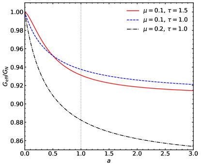
Figure 2: The comparison of Planck masses via $G_{\mathrm{eff}}/G_{N}=G_{\mathrm{matter}}=G_{\mathrm{light}}$, for the indicated values of $\mu$ and $\tau$, with fixed $a_{t}=0.5$. We can verify that at very early–times $(a\rightarrow 0)$, $M_{*}\simeq m_{p}$.

In the following analysis, we will be considering the inferred dark energy parameter constraints from upcoming detections of standard sirens, using a specific modified gravity model; the No Slip Gravity model 5 . No Slip Gravity is a special subclass model of the Horndeski gravitational framework Horndeski:1974wa ; Deffayet:2011gz , which is well–known to be the most general scalar–tensor theory having second–order field equations in four dimensions. This framework encompasses 15 , for instance, $f(R)$ models DeFelice:2010aj , quintessence Tsujikawa:2013fta , the Brans–Dicke model Brans:1961sx , and covariant Galileons Deffayet:2009wt .

The No Slip Gravity model is advantageous to study in the sense that gravitational waves propagate at the same speed of light. Recent results from the binary neutron star merger GW170817/GRB 170817A have shown that the speed of propagation of GWs ($c_{\mathrm{GW}}$) is in an excellent agreement with the speed of light ($c$), such that $|(c_{\mathrm{GW}}-c)/c|\lesssim\mathcal{O}(10^{-15})$ 12 . The No Slip Gravity model is therefore a viable model which naturally satisfies this requirement, as opposed to a number of well–known modified theories of gravity which were adversely affected by this measurement (see, for instance, Ezquiaga:2017ekz ; Sakstein:2017xjx ; Amendola:2017orw ; Crisostomi:2017pjs ; Baker:2017hug ; Ezquiaga:2018btd ; Kase:2018aps ).

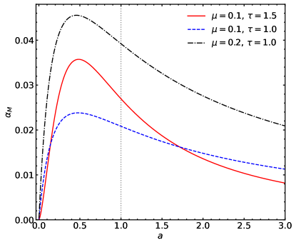
Figure 3: Comparison plot of $\alpha_{M}$, for the indicated values of $\mu$ and $\tau$, with fixed $a_{t}=0.5$. The grey vertical line indicates the corresponding $\alpha_{M}^{0}$ values.

The gravitational effect on matter and photons can be analysed via the modified Poisson equations which relate the time–time metric potential with the space–space metric potential. The growth of cosmic structure is governed by the gravitational strength $G_{\mathrm{matter}}$, while the deflection of light is characterised by the gravitational strength $G_{\mathrm{light}}$. The offset between the latter gravitational strengths is referred to as the gravitational slip parameter, defined by

$$\bar{\eta}=\frac{G_{\mathrm{matter}}}{G_{\mathrm{light}}}\;,$$ (10)

such that $\bar{\eta}=1$ corresponds to vanishing slip, which holds in the case of the concordance model of cosmology. In this modified gravity model, we have a simple relationship between the Planck mass running parameter $\alpha_{M}$, and the kinetic braiding parameter $\alpha_{B}$ (see Bellini:2014fua for further information on the Horndeski property functions $\alpha_{M,B}$). Indeed, the no slip condition is specified by $\alpha_{B}=-2\alpha_{M}$, which then determines the ratio between the constant Planck mass $(m_{p})$ in Einstein gravity, and the effective time–dependent Planck mass in modified gravity $M_{\ast}$, which is given by

$$G_{\mathrm{matter}}=G_{\mathrm{light}}=\frac{m_{p}^{2}}{M_{*}^{2}}\;.$$ (11)

We should remark that a consequence of the stability conditions within this framework, the gravitational strength is found to be diluted with respect to the standard prediction, leading to weaker gravity. This atypical feature of scalar–tensor theories of gravity arises from the fact that the non–null kinetic braiding parameter mixes the scalar sector into the tensor sector, and such a feature could address possible anomalies in growth of structure observations Hildebrandt:2016iqg ; Joudaki:2017zdt ; Abbott:2017wau ; Troxel:2017xyo .

When considering the propagation of GWs, it is essential that we infer the luminosity distance of the source, $D_{L,\mathrm{GW}}$. The standard luminosity distance for electromagnetic sources will be denoted by $D_{L,\mathrm{GR}}$, such that

$$D_{L,\mathrm{GR}}(z)=c(1+z)\int^{z}_{0}\frac{\mathrm{d}z^{\prime}}{H(z^{\prime})}\;,$$ (12)

with

$$H^{2}(z)=H_{0}^{2}\left[\frac{\Omega_{m}^{0}}{a^{3}}+\frac{(1-\Omega_{m}^{0})}{a^{3}}\left(a^{-3(w_{0}+w_{a})}e^{3[w_{a}(a-1)]}\right)\right]\;,$$ (13)

where we recall that $H_{0}$ and $\Omega_{m}^{0}$ denote the Hubble constant and the current matter density fraction, respectively. For the dark energy parameter choice of ${(w_{0},\,w_{a})}={(-1,\,0)}$, i.e. the concordance model of cosmology, the above relation for $H(z)$ reads as follows

$$H^{2}(z)=H_{0}^{2}\left[\Omega_{m}^{0}(1+z)^{3}+(1-\Omega_{m}^{0})\right]\;,$$ (14)

for a spatially–flat FLRW metric. In the rest of the paper, unless explicitly mentioned, $D_{L}$ will be denoting $D_{L,\mathrm{GR}}$.

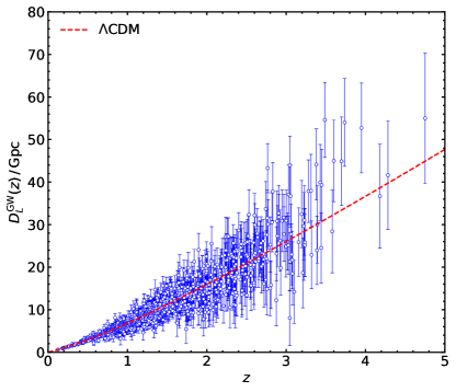
Figure 4: Luminosity distance distribution of the GW data as a function of redshift. There are a total of $1000$ GW candidates.

The relationship between the GW standard siren luminosity distance and the photon standard candle luminosity distance, is given by eq15a ; eq15b ; Nishizawa:2017nef ; 13 ; 14 ,

$$\frac{D_{L,\mathrm{GW}}(z)}{D_{L,\mathrm{GR}}(z)}=\exp{\left\{-\int_{0}^{z}\frac{\mathrm{d}z^{\prime}}{1+z^{\prime}}\delta(z^{\prime})\right\}}\;.$$ (15)

We will now consider the determination of $\{M_{*},\,\alpha_{M}\}$ by adopting the parametrisations as reported in 5 , which is explicitly given by

$$\left(\frac{m_{p}}{M_{*}}\right)^{-2}=1+\frac{\mu}{1+\left(a/a_{t}\right)^{-\tau}}\;,$$ (16)

where $\mu$ is the amplitude of the transition from the early Universe to the asymptotic future, and $a_{t}$ is the scale factor when this occurs, with $0<\tau\leq 3/2$ being its rapidity. In Figure 2 we illustrate three comparisons of the Planck mass with the time–dependent effective Planck mass according to the parameter values as specified in Table 1. We can verify that, asymptotically the effective running Planck mass tends to the constant Planck mass; this is justified since in the early Universe they are expected to be identical.

By using the fact that $\alpha_{M}=\mathrm{d}\ln M_{\ast}^{2}/\mathrm{d}\ln a$, we get to the following parametrisation of the Planck mass running parameter

$$\alpha_{M}=\left[1+\frac{\mu}{1+e^{-\tau(\ln a-\ln a_{t})}}\right]^{-1}\frac{\tau\mu e^{-\tau(\ln a-\ln a_{t})}}{\left[1+e^{-\tau(\ln a-\ln a_{t})}\right]^{2}}\;.$$ (17)

The redshift evolution of $\alpha_{M}$ is depicted in Figure 3, for the specified parameter values listed in Table 1. In order to solve equation (15), we need to find an expression for $\delta(z)$. 16 has provided a generic parametric form of $\delta(z)$, suitable for most of the modified gravity models,

$$\delta(z)=\frac{n(1-\zeta_{0})}{1-\zeta_{0}+\zeta_{0}(1+z)^{n}}\;,$$ (18)

where $\zeta_{0}$ and $n$ for Horndeski specific models are defined by

$$\zeta_{0} = \lim_{z\to\infty}\frac{M^{*}(0)}{M^{*}(z)}\;,$$ (19)

$$n \simeq \frac{\alpha_{M0}}{2(\zeta_{0}-1)}\;.$$ (20)

We can see that at early–times ($z\rightarrow\infty$) we recover Einstein gravity with $\delta(z)\rightarrow 0$, while at late–times ($z\ll 1$), $\delta(z)\simeq n(1-\zeta_{0})$. $\zeta_{0}=1$ corresponds to the standard prediction, thus the two luminosity distances are identical, $D_{L,\mathrm{GW}}=D_{L,\mathrm{GR}}$.

IV Analysis

IV.1 Data

We will present a comparison of our results obtained from using the luminosity distance estimates using the modified gravity model, to the ones derived from assuming a standard electromagnetic source luminosity distance. For computing the latter case, we used the simulation data of 17 . We refer the reader to this work for further details on the characteristics of the data.

IV.2 Errors

For Fisher matrix analysis nla.cat-vn81100 ; Cutler:1994ys ; Berti:2004bd , we need to model the systematic errors and account for the cosmological uncertainties propagating through the luminosity distance measurement. The uncertainties ($\sigma$) in luminosity distance measurement error $\langle\delta D_{L}\rangle$ is composed of

$$\langle\sigma\rangle^{2}=\langle\sigma_{\mathrm{photo-z}}\rangle^{2}+\langle\sigma_{WL}\rangle^{2}+\langle\sigma_{I}\rangle^{2}+\langle\sigma_{P}\rangle^{2}\;,$$ (21)

where the four terms on the right–hand side stand for the photometric redshift measurement error, weak lensing error, instrumental error and the peculiar velocity error.

• Redshift error : Since most of distant binaries will have photometric redshift, it is essential to account for the photometric redshift measurement error. It is modelled by Tamanini:2016zlh ; 19 ; 20

  $$\sigma_{\mathrm{photo-z}}=\left(\frac{\partial D_{L}}{\partial z}\right)\left[0.03(1+z)\right]\;.$$ (22)

  It is vital, that of all the sources which will be detected, the fraction of counterparts identifiable with the availability of spectroscopic redshift should have a significant effect on the parameter estimation and the improvement of the constraints. For the spectroscopic redshift sources, we assume a flat error of $0.001$ Congedo:2018wfn . Even with current ongoing large scale SNe surveys, mitigating the systematic errors originating from high–redshift photometric samples is a challenge in itself. Assuming there will be vast improvement in observing capabilities in the next one–to–two decades in redshift measurements, we will present a comparison of the results based on scenarios, of different level of expected detections of the spectroscopic redshift.
  

  $\alpha_{M}^{0}$	$\zeta_{0}$	n
  0.0270	1.0363	0.3715
  0.0208	1.0328	0.3176
  0.0392	1.0646	0.3036

  Table 2: We here summarise the fit parameters which are necessary for the computation of the luminosity distances in our modified gravity model. These have been inferred from equation (15) along with the specified values in Table 1.

• Instrumental error : The combined SNR for the proposed ET’s network of three independent interferometers is given by

  $$\rho=\sqrt{\sum_{i=1}^{3}\left(\rho^{(i)}\right)^{2}}\;,$$ (23)

  where $\rho^{(i)}=\sqrt{\langle\widehat{\mathcal{H}}^{(i)},\widehat{\mathcal{H}}^{(i)}\rangle}$, with the standard inner product expressed as follows

  $$\langle a,\,b\rangle=4\int_{f_{\mathrm{lower}}}^{f_{\mathrm{upper}}}\frac{\hat{a}(f)\hat{b}^{\ast}(f)+\hat{a}^{\ast}(f)\hat{b}(f)}{2}\frac{\mathrm{d}f}{S_{h}(f)}\;.$$ (24)

  The noise power spectral density of the ET is denoted by $S_{h}(f)$, and is illustrated in Figure 1. The upper cutoff frequency is dictated by the last stable orbit of the binary system 6 , while the lower cutoff frequency is set to $1\,\mathrm{Hz}$. Following the adopted SNR threshold for the current GW detectors, we consider a GW detection if the three ET interferometers have a network SNR of $\rho_{\mathrm{net}}>8$. Assuming that the error on $D_{L,\mathrm{GW}}$ is uncorrelated with any other GW parameter, we can estimate the instrumental error via a Fisher information matrix, leading to the following expression

  $$\sigma_{I}\simeq\sqrt{\Bigg{\langle}\frac{\partial\widehat{\mathcal{H}}}{\partial D_{L,\mathrm{GW}}},\frac{\partial\widehat{\mathcal{H}}}{\partial D_{L,\mathrm{GW}}}\Bigg{\rangle}^{-1}}\;.$$ (25)

  Moreover, since $\widehat{\mathcal{H}}\propto D_{L,\mathrm{GW}}^{-1}$, we arrive at $\sigma_{I}\simeq 2D_{L,\mathrm{GW}}/\rho$, where the factor of two was introduced in order to take into account the maximal effect of the binary’s inclination angle on the SNR. We should also remark that one could adopt the following fitting function for the projected instrumental error contribution of the ET to the relative error on the luminosity distance measurement 6

  $$\sigma_{I}=0.1449z-0.0118z^{2}+0.0012z^{3}\;.$$ (26)

• Weak lensing error : It is introduced, since standard sirens get lensed in identical fashion to EM sources, the inhomogeneities along the line–of–sight give rise to a weak lensing effect. In the weak lensing regime, the magnification $\mu_{WL}$ can be expressed to first order in terms of the convergence $\kappa$ as

  $$\mu_{WL}\simeq 1+2\kappa\;.$$ (27)

  Therefore, we will adopt the following weak lensing uncertainty wlerror

  $$\sigma_{WL}=\frac{0.1z}{1+0.07z}\;.$$ (28)

• Peculiar velocity error : The peculiar velocity of the source relative to the Hubble flow introduces another additional error. We consider the following functional form for this error 18

  $$\sigma_{P}^{2}=\left[1+\frac{c(1+z)^{2}}{H(z)D_{L}}\right]^{2}\frac{\langle v^{2}\rangle}{c^{2}}\;,$$ (29)

  where we assume a r.m.s. velocity of $\langle v\rangle=500\ \rm km/s$ based on numerical simulation results from 21 .

We are now in a position to write down the Fisher matrix for the cosmological parameters of our given model, which can be expressed as follows

$$F_{ij}=\sum_{n=1}^{1000}\frac{1}{(\sigma^{2})_{n}}\left.\frac{\partial D_{L}(z_{n})}{\partial\theta_{i}}\right|_{\rm fid}\left.\frac{\partial D_{L}(z_{n})}{\partial\theta_{j}}\right|_{\rm fid}\;,$$ (30)

where the sum runs over all the $1000$ standard siren events. The partial derivatives of $D_{L}$ (equation (12)) are with respect to the cosmological parameters $\Theta=\{\Omega_{m}^{0},\,H_{0},\,w_{0},\,w_{a}\}$, computed at their fiducial values $\Theta_{\mathrm{fid}}=\{0.315,\,67.4,\,-1,\,0\}$, adopted from the latest CMB inferred constraints Aghanim:2018eyx in the $\Lambda$CDM framework.

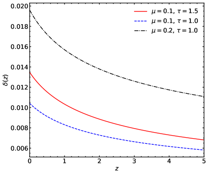
Figure 5: The redshift evolution of the $\delta(z)$ function, for the specified parameters as indicated in Table 1.

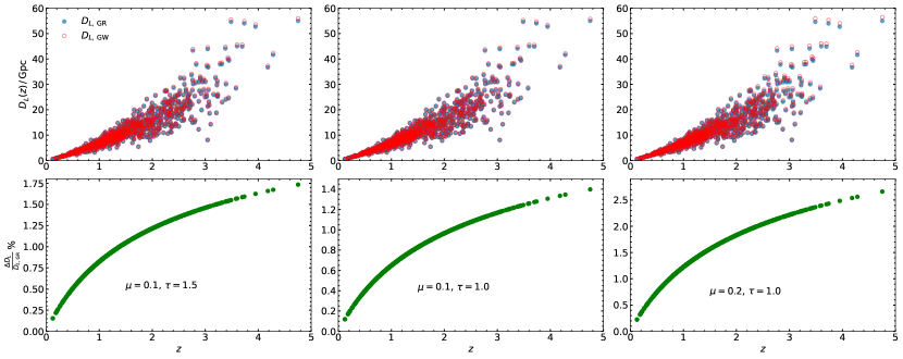
Figure 6: Comparison between $D_{L,\,\mathrm{GW}}$ and $D_{L,\,\mathrm{GR}}$, where the former is computed via equation (15). The lower panel shows the relative error between the two luminosity distances.

V Results

As mentioned above, for our Horndeski model analysis, we used the No Slip Gravity model. For the Fisher analysis, we have to choose the parametric results of the model parameters. Precisely, we needed the value of the parameters $(\zeta_{0},\,n)$ and for that we also needed the value of $\alpha_{M}^{0}$ (equations (19, 20)). It is evident that for the computation of the above parameters, via equations (16, 17, 18), we need to know $\tau,\,\mu$ and $a_{t}$. 5 has presented three different sets of viable parameter values of $\tau$ and $\mu$ for a fixed $a_{t}=0.5$, which we summarise in Table 1. By adopting these parameter sets, we computed three respective sets of $\alpha_{M}^{0}$ along with the corresponding values of $\zeta_{0}$ and $n$ using equation (19) together with equation (20). The derived values are summarised in Table 2.

It is interesting to note that 16 proposed fit values for the above parameters using another alternate modified gravity model, the RR model, which is specified by

$$[\zeta_{0},\,n]=[0.970,\,2.5]\;.$$ (31)

In appendix A, we further present a comparison of our results with this model parametrisation.

V.1 Luminosity Distance

In this section, we will present a comparison of the computed luminosity distances ($D_{L,\,\mathrm{GW}}$) using the parameter values as specified in Tables 1–2 with the luminosity distances from Einstein gravity ($D_{L,\,\mathrm{GR}}$). Based on equation (15), we calculated $\delta(z)$ from the parameter sets outlined in the previously mentioned tables. The different redshift evolution of $\delta(z)$ for different models are shown in Figure 5.

Moreover, Figure 6 shows a comparison of the distance estimates from three sets of parameter values. One could observe that distance estimates are more sensitive to the amplitude of transition parameter $\mu$, compared to the rapidity $\tau$.

V.2 Fisher Analysis

In 5 the combination of $\left[\mu,\,\tau,\,a_{t}\right]=\left[0.1,\,0.5,\,1.5\right]$ was found to be in good agreement with current observations. In this section we will present a comparison of the $1-\sigma$ constraint plot (ellipses) on the dark energy equation of state parameters $w_{0}-w_{a}$ under the assumption of all three previously defined parameter sets. In Figure 7 the three different parameter choices are considered, with each of them being analysed in four distinct spectroscopic redshift availability criteria. Three of the four spectroscopic redshift coverage ranges are chosen as $z_{\mathrm{spectro}}=[0.2,\,0.3,\,0.5]$, and as a hypothetical benchmark result we showed what is the constraint if there was a (hypothetical) full spectroscopic redshift coverage. At the time of writing this paper, our best guess is to assume that up to redshift of $z\simeq 0.3$, there will be possible spectroscopic observations and thus the availability of the spectroscopic redshift. The concentric ellipses in each plot, from outside to inside, cover $z_{\mathrm{spectro}}=[0.3-4.0]$ cases. Each of these cases are plotted in pairs of ellipses from the No Slip Gravity model and the corresponding Einstein gravity model. We can clearly notice that there is a degeneracy in our results between the three parameter combinations. In all considered cases, the No Slip Gravity model is found to be closely related with Einstein gravity inferred results. As expected, the constraints get tighter as we increase the spectroscopic coverage.

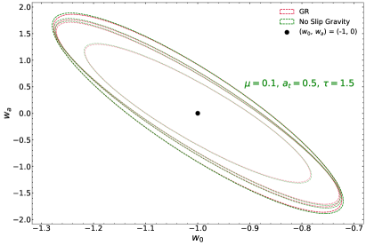
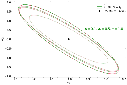
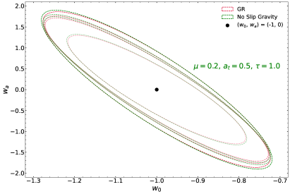
Figure 7: Fisher ellipses computed by using the luminosity distances $D_{L,\,\mathrm{GW}}$ for each respective parameter set in the No Slip Gravity model (green), compared with the ellipse derived from $D_{L,\,\mathrm{GR}}$ (red). Each panel has a set of four concentric ellipse pairs, which correspond to the $z_{\mathrm{spectro}}$ coverage from $[0.2-4.0]$ as we traverse from outside to inside.

A measure of these constraints can be analysed by using the Figure of Merit (FOM) values 28 . In Table 3 we have summarised the FOM values of the ellipses found in Figure 7, and these are further illustrated in Figure 8. There is consistency in the trend of the FOM values throughout the three parameter combinations as a function of the spectroscopic redshift coverage. We also observe that there is a remarkable improvement in the FOM as we increase the spectroscopic redshift from $0.2$ to $0.3$. In contrast, the improvement in the FOM for the remaining length of the abscissa is less steeper. Definitely, at the time of ET’s realisation, we expect this redshift range to be spectroscopically covered. The blue dashed line gives a locus of the FOM as a function of the spectroscopic redshift coverage, all the way to full spectroscopic redshift availability. Significant improvements can be made by focusing on the enhancement of spectroscopic redshift availability in the low–redshift ranges. We should further remark that there is no significant model sensitivity in terms of the FOM, although visibly minuscule deviations could be noticed at the highest redshift coverage between Einstein gravity and the No Slip Gravity models.

$z_{\rm spectro}$	FOM	Set
0.2	0.4283	GR
0.3	0.5066
0.5	0.5405
0.2	0.4231	NSG-I
0.3	0.5000
0.5	0.5332
0.2	0.4242	NSG-II
0.3	0.5014
0.5	0.5348
0.2	0.4206	NSG-III
0.3	0.4969
0.5	0.5298

Table 3: Summary of the FOM values of the plots shown in Figure 7, as a function of the spectroscopic redshift availability ($z_{\rm spectro}$) excluding the case of full spectroscopy, i.e. $[0.2,\,0.3,\,0.5]$. The third column corresponds to either Einstein gravity (GR) or the adopted No Slip Gravity (NSG) parameter values, such that $\rm{NSG-I}:(\mu=0.1,\,\tau=1.5),\ \rm{NSG-II}:(\mu=0.1,\,\tau=1.0)$ and $\rm{NSG-III}:(\mu=0.2,\,\tau=1.0)$. A visual representation is depicted in Figure 8.

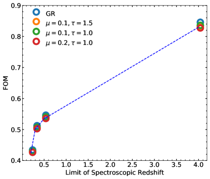
Figure 8: The FOM of the confidence regions shown in Figure 7 (Table 3) as a function of the spectroscopic redshift coverage. The blue dashed line corresponds to the mean FOM of the four values at each $z_{\mathrm{spectro}}$.

V.3 MCMC analysis

We also conducted a Markov Chain Monte Carlo (MCMC) analysis with the forecast data, to determine how well the parameters $\zeta_{0}$ and $n$ could be measured with this data, and what degeneracies might exist with the cosmological parameters that control cosmic distances.

We use the affine-invariant ensemble sampler for MCMC GoodmanWeare , applying the specific Python implementation emcee 2013PASP..125..306F . We adopted uniform priors, with $0<\Omega_{m}^{0}<1$, $0<\zeta_{0}<2$, and $-1<n<2$. We assume a flat universe and hold all other parameters fixed to their fiducial values, including the dark energy parameters $w_{0}=-1$ and $w_{a}=0$. We ran separate MCMC analyses for each of the four models, to determine if the data could distinguish between the models (assuming each of them to be true). The Bayesian credible contours are shown in Figure 9, and were generated using ChainConsumer 2016JOSS….1…45H .

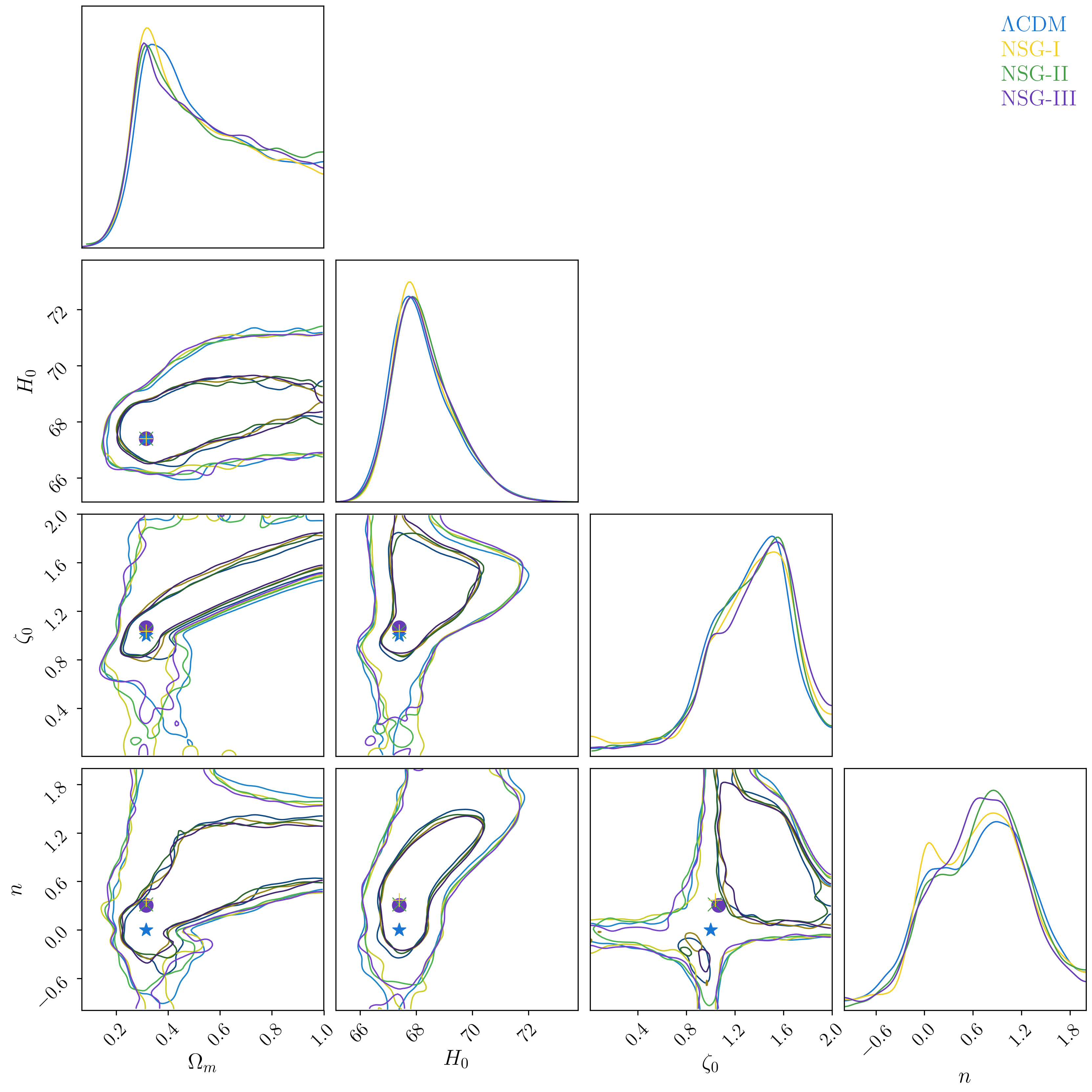
Figure 9: The forecasted 68% and 95% Bayesian credible intervals for the parameters $H_{0}$, $\Omega_{m}^{0}$, $\zeta_{0}$ and $n$, using the prospective data described in section IV, for each of the four different underlying models ($\Lambda$CDM where gravity is the Einstein model, and three No Slip Gravity models with different choices of $\zeta_{0}$ and $n$). The bounds are estimated using MCMC, and the different markers represent the values of the parameters for the true model, in the different cases. The bounds on the No Slip gravity parameters are much larger than the differences in the true values of $\zeta_{0}$ and $n$, and there are significant parameter degeneracies between $\Omega_{m}^{0}$ and the No Slip gravity parameters. The constraints are nearly identical between the models using this data set.

We find that the data is not constraining enough to be able to to distinguish between the different models. The difference between values of $\zeta_{0}$ and $n$ given in Table 2 is much smaller than the parameter bounds, and so the models are indistinguishable. The constraints on these parameters are also identical, confirming the results from section V.2.

We see a significant degeneracy between the No Slip gravity model parameters $\zeta_{0}$ and $n$, and the matter density $\Omega_{m}^{0}$. As the matter density increases, the luminosity distance to the different GW sources will decrease, but this can be balanced by increasing the amount of GW ‘dimming’ that is generated by the modified gravity model, making the sources appear to be further away. This degeneracy is also present between the No Slip gravity parameters and $H_{0}$, though to a lesser extent. Since the Hubble parameter is mainly constrained by the data at low redshift, the amount of distance available to see a significant impact on the value of $H_{0}$ is reduced. This is why the values of $n$ and $\zeta_{0}$ need to be quite large before the Hubble parameter is significantly shifted.

Though the model cannot be distinguished from Einstein gravity using this data by itself, it may be possible to do so in combination with other distance probes. Since luminosity distances (and angular diameter distances) measured by electromagnetic means (for example, SNe Ia or BAO) will be completely insensitive to the No Slip gravity model parameters, they can provide independent constraints on the cosmological parameters $H_{0}$ and $\Omega_{m}^{0}$. By combining these electromagnetic data sets with the GW luminosity distances, the degeneracy between the cosmology parameters $\Omega_{m}^{0}$ and $H_{0}$ with the No Slip gravity parameters $\zeta_{0}$ and $n$ can be broken, and the size of the confidence contour can be significantly reduced. This is analogous to testing Etherington’s distance-duality equation for electromagnetic distances, with the alteration that here the check is the consistency between electromagnetic and GW distances. We leave such a demonstration for future work.

VI Conclusion

We have presented a study of what we can expect in terms of cosmological analysis from prospective GW detections from the perspective of modified gravity models, particularly focusing on a subclass of the Horndeski scalar–tensor theory of gravitation. We have presented a comparison to compare the cases between a modified gravity model and the standard Einstein gravity. For the implementation of the modified gravity model, we used the No Slip Gravity model, as outlined in 5 . This is primarily motivated from the fact that current observational probes, including GW detections, are in agreement with the predictions of the No Slip Gravity model. Third generation interferometric surveys are projected to be operational post $2030$ and we expect that modified gravity models, including the one analysed here, will be robustly tested by a number of proposed surveys such as LSST 2009arXiv0912.0201L and Euclid 2011arXiv1110.3193L .

From our results, we see that the alternative model mimics the standard Einstein theory for the homogeneous expansion. We find, for the models explored here, that the effect on both the distances measured, and the values of the cosmological parameters recovered, are small. We show that, considering a GW-only data set, there will be significant parameter degeneracies between the cosmological parameters, such as $\Omega_{m}^{0}$, with the parameters of the No Slip gravity model. This is because the ‘dimming’ of the GW luminosity distance can also be mimicked by the change in propagation of the GW in the modified gravity theory. Such a degeneracy could be broken through combining the GW dataset with distances estimated through electromagnetic means, or else through separate constraints on the No Slip gravity model parameters.

We await with great expectations from future GW surveys for demystifying the fabric of gravity and the implications it will have on improving our understanding of precision cosmology.

VII Acknowledgement

We are grateful to the authors of 17 for providing their mock data set. AM acknowledges the support of Orau Grant No. 110119FD4534. JM would like to acknowledge funding support Cosmology@MALTA which is supported by the University of Malta. DFM thanks the Research Council of Norway for their support and the UNINETT Sigma2 – the National Infrastructure for High Performance Computing and Data Storage in Norway.

Appendix A Comparison with the RR Model.

16 have presented an alternate parametrisation for a different modified gravity model, the RR model (for a detailed study, refer to 16 ; 22 ).

Although these models, are mostly screened from observational requirements, still for comparisons and reference purposes, we show the similar $1-\sigma$ dark energy parameter constraint plot from this model, with $[\zeta_{0},\,n]=[0.970,\,2.5]$ (equation 31). It is interesting to see that the RR model gives rise a constraint which is marginally tighter than the corresponding Einstein gravity model. A measure of their corresponding FOM is also provided in the inset plot of Figure 10.

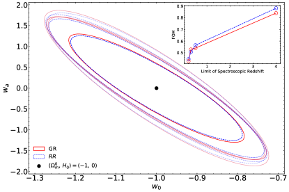
Figure 10: Constraint plots for the RR Gravity model (blue) in comparison with the Einstein gravity confidence regions (GR, red) for dark energy parameters $(w_{0},\,w_{a})$. The concentric ellipse pairs are plotted similar to those in Figure 7, where we used the assumption that there will be spectroscopic redshifts available up to $z=[0.2,\,0.3,\,0.5,\,4.0]$ (outside to inside). Inset plot: FOM plot of the corresponding ellipses.

Appendix B Hubble Parameter Constraints with the No Slip Gravity Model

We here present the $H_{0}-\Omega_{m}^{0}$ constraint figures. The concentric pairs of ellipses are plotted similar to those in Figure 7 as a function of the spectroscopic redshift availability [$0.2$ (second from the outermost), $0.3$, $0.5$, $4.0$ (innermost)]. For No Slip Gravity we used the first parameter choice of $\left[\mu,\,\tau,\,a_{t}\right]=\left[0.1,\,0.5,\,1.5\right]$. The outermost light blue ellipse is a reference showing the constraint if no spectroscopic redshifts are available.

Similar to the observations on the $w_{0}-w_{a}$ confidence regions, we see that huge improvements in parameter constraints can be achieved by using spectroscopic redshifts in the low–redshift range. Indeed, the inset plot of the FOM from Figure 11 (or Table 3) shows this trend. We also see that the modified gravity model closely mimics the standard prediction and that they are nearly identical. Again, we would like to remark that the case of full spectroscopic redshift availability is a hypothetical reference point. This can be thought of as the maximal constraint that these parameter pairs can achieve with the given specifications.

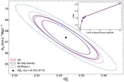
Figure 11: Comparison plot showing the extreme limits of the constraints on the Hubble constant ($H_{0}$) and the matter density ($\Omega_{m}^{0}$) plane using the first parameter set (blue dashed) of the No Slip Gravity model from Table 1 along with Einstein gravity (GR) (red dashed). As we move from the outer edge to the inner edge, the spectroscopic coverage changes from $[0.2-4.0]$, and the dot–dashed blue confidence region corresponds to the scenario if all redshift was photometric (using GR). Inset plot: FOM of the corresponding ellipses, also listed in Table 4.

$\rm z_{spectro}$	$\rm GR$	$\rm NSG-I$
0.0	0.7555	0.7689
0.2	1.2981	1.2880
0.3	1.5077	1.4953
0.5	1.6055	1.5918
4.0	2.5614	2.5377

Table 4: Table showing the FOM comparisons between GR and the No Slip Gravity model from Figure 11. The second column is similar in abbreviation to Table 3.

References

- [1] Adam G. Riess et al. Observational evidence from supernovae for an accelerating universe and a cosmological constant. Astron. J., 116:1009–1038, 1998.
- [2] S. Perlmutter et al. Measurements of and from 42 high redshift supernovae. Astrophys. J., 517:565–586, 1999.
- [3] M. Kowalski et al. Improved Cosmological Constraints from New, Old and Combined Supernova Datasets. Astrophys. J., 686:749–778, 2008.
- [4] Bernard F. Schutz. Determining the Hubble Constant from Gravitational Wave Observations. Nature, 323:310–311, 1986.
- [5] Masamune Oguri. Measuring the distance-redshift relation with the cross-correlation of gravitational wave standard sirens and galaxies. Phys. Rev. D, 93(8):083511, 2016.
- [6] Xuheng Ding, Marek Biesiada, Xiaogang Zheng, Kai Liao, Zhengxiang Li, and Zong-Hong Zhu. Cosmological inference from standard sirens without redshift measurements. JCAP, 04:033, 2019.
- [7] The LIGO Scientific Collaboration, the Virgo Collaboration, B. P. Abbott, and Abbott. A gravitational-wave measurement of the Hubble constant following the second observing run of Advanced LIGO and Virgo. arXiv e-prints, page arXiv:1908.06060, August 2019.
- [8] Suvodip Mukherjee, Benjamin D. Wandelt, Samaya M. Nissanke, and Alessandra Silvestri. Accurate and precision Cosmology with redshift unknown gravitational wave sources. arXiv e-prints, page arXiv:2007.02943, July 2020.
- [9] Hai Yu, Pengjie Zhang, and Fa-Yin Wang. Strong lensing as a giant telescope to localize the host galaxy of gravitational wave event. Mon. Not. Roy. Astron. Soc., 497(1):204–209, 2020.
- [10] B.P. Abbott et al. Observation of Gravitational Waves from a Binary Black Hole Merger. Phys. Rev. Lett., 116(6):061102, 2016.
- [11] B.P. Abbott et al. GW170817: Observation of Gravitational Waves from a Binary Neutron Star Inspiral. Phys. Rev. Lett., 119(16):161101, 2017.
- [12] Stephen Fairhurst. Triangulation of gravitational wave sources with a network of detectors. New J. Phys., 11:123006, 2009. [Erratum: New J.Phys. 13, 069602 (2011)].
- [13] Benjamin P Abbott et al. Exploring the Sensitivity of Next Generation Gravitational Wave Detectors. Class. Quant. Grav., 34(4):044001, 2017.
- [14] M. Punturo et al. The Einstein Telescope: A third-generation gravitational wave observatory. Class. Quant. Grav., 27:194002, 2010.
- [15] M. Punturo, M. Abernathy, et al. The third generation of gravitational wave observatories and their science reach. Classical and Quantum Gravity, 27(8):84007, April 2010.
- [16] Shang-Jie Jin, Dong-Ze He, Yidong Xu, Jing-Fei Zhang, and Xin Zhang. Forecast for cosmological parameter estimation with gravitational-wave standard siren observation from the Cosmic Explorer. JCAP, 03:051, 2020.
- [17] Pau Amaro-Seoane, Heather Audley, et al. Laser Interferometer Space Antenna. arXiv e-prints, page arXiv:1702.00786, February 2017.
- [18] Pau Amaro-Seoane et al. eLISA/NGO: Astrophysics and cosmology in the gravitational-wave millihertz regime. GW Notes, 6:4–110, 2013.
- [19] Jun Luo et al. TianQin: a space-borne gravitational wave detector. Class. Quant. Grav., 33(3):035010, 2016.
- [20] Giuseppe Congedo and Andy Taylor. Joint cosmological inference of standard sirens and gravitational wave weak lensing. Phys. Rev. D, 99(8):083526, 2019.
- [21] Xuan-Neng Zhang, Ling-Feng Wang, Jing-Fei Zhang, and Xin Zhang. Improving cosmological parameter estimation with the future gravitational-wave standard siren observation from the Einstein Telescope. Phys. Rev. D, 99(6):063510, 2019.
- [22] Ling-Feng Wang, Xuan-Neng Zhang, Jing-Fei Zhang, and Xin Zhang. Impacts of gravitational-wave standard siren observation of the Einstein Telescope on weighing neutrinos in cosmology. Phys. Lett. B, 782:87–93, 2018.
- [23] Enis Belgacem, Yves Dirian, et al. Cosmology and dark energy from joint gravitational wave-GRB observations. JCAP, 08:015, 2019.
- [24] Rong-Gen Cai and Tao Yang. Estimating cosmological parameters by the simulated data of gravitational waves from the Einstein Telescope. Phys. Rev. D, 95(4):044024, 2017.
- [25] Kai Liao, Xi-Long Fan, Xu-Heng Ding, Marek Biesiada, and Zong-Hong Zhu. Precision cosmology from future lensed gravitational wave and electromagnetic signals. Nature Commun., 8(1):1148, 2017. [Erratum: Nature Commun. 8, 2136 (2017)].
- [26] N. Aghanim, Y. Akrami, M. Ashdown, J. Aumont, C. Baccigalupi, M. Ballardini, A. J. Banday, R. B. Barreiro, N. Bartolo, and et al. Planck 2018 results. VI. Cosmological parameters. Astronomy & Astrophysics, 641:A6, Sep 2020.
- [27] Rocco D’Agostino and Rafael C. Nunes. Probing observational bounds on scalar-tensor theories from standard sirens. Phys. Rev. D, 100(4):044041, 2019.
- [28] Weiqiang Yang, Supriya Pan, Eleonora Di Valentino, Bin Wang, and Anzhong Wang. Forecasting Interacting Vacuum-Energy Models using Gravitational Waves. JCAP, 05:050, 2020.
- [29] W. Zhao, C. van den Broeck, D. Baskaran, and T. G. F. Li. Determination of dark energy by the Einstein Telescope: Comparing with CMB, BAO, and SNIa observations. Phys. Rev. D, 83(2):023005, January 2011.
- [30] Weiqiang Yang, Sunny Vagnozzi, Eleonora Di Valentino, Rafael C. Nunes, Supriya Pan, and David F. Mota. Listening to the sound of dark sector interactions with gravitational wave standard sirens. JCAP, 07:037, 2019.
- [31] Jing-Fei Zhang, Hong-Yan Dong, Jing-Zhao Qi, and Xin Zhang. Prospect for constraining holographic dark energy with gravitational wave standard sirens from the Einstein Telescope. Eur. Phys. J. C, 80(3):217, 2020.
- [32] William J. Wolf and Macarena Lagos. Standard Sirens as a Novel Probe of Dark Energy. Phys. Rev. Lett., 124(6):061101, 2020.
- [33] Weiqiang Yang, Supriya Pan, David F. Mota, and Minghui Du. Forecast constraints on Anisotropic Stress in Dark Energy using gravitational-waves. Mon. Not. Roy. Astron. Soc., 497(1):879–893, 2020.
- [34] Riis R.A. Bachega, André A. Costa, E. Abdalla, and K.S.F. Fornazier. Forecasting the Interaction in Dark Matter-Dark Energy Models with Standard Sirens From the Einstein Telescope. JCAP, 05:021, 2020.
- [35] Hai-Li Li, Dong-Ze He, Jing-Fei Zhang, and Xin Zhang. Quantifying the impacts of future gravitational-wave data on constraining interacting dark energy. JCAP, 06:038, 2020.
- [36] Atsushi Nishizawa. Generalized framework for testing gravity with gravitational-wave propagation. I. Formulation. Phys. Rev. D, 97(10):104037, 2018.
- [37] B.S. Sathyaprakash, B.F. Schutz, and C. Van Den Broeck. Cosmography with the Einstein Telescope. Class. Quant. Grav., 27:215006, 2010.
- [38] B.P. Abbott et al. Gravitational Waves and Gamma-rays from a Binary Neutron Star Merger: GW170817 and GRB 170817A. Astrophys. J. Lett., 848(2):L13, 2017.
- [39] Tao Yang, Bin Hu, Rong-Gen Cai, and Bin Wang. New probe of gravity: strongly lensed gravitational wave multi-messenger approach. Astrophys. J., 880:50, 2019.
- [40] Minghui Du, Weiqiang Yang, Lixin Xu, Supriya Pan, and David F. Mota. Future constraints on dynamical dark-energy using gravitational-wave standard sirens. Phys. Rev. D, 100(4):043535, 2019.
- [41] Macarena Lagos, Maya Fishbach, Philippe Landry, and Daniel E. Holz. Standard sirens with a running Planck mass. Phys. Rev. D, 99(8):083504, 2019.
- [42] Enis Belgacem, Stefano Foffa, et al. Gaussian processes reconstruction of modified gravitational wave propagation. Phys. Rev. D, 101(6):063505, 2020.
- [43] Zhuo Chen, E. A. Huerta, Joseph Adamo, et al. Observation of eccentric binary black hole mergers with second and third generation gravitational wave detector networks. arXiv e-prints, page arXiv:2008.03313, August 2020.
- [44] Ashish Sharma and Jan Harms. Searching for cosmological gravitational-wave backgrounds with third-generation detectors in the presence of an astrophysical foreground. Physical Review D, 102(6), Sep 2020.
- [45] S. Mastrogiovanni, D. Steer, and M. Barsuglia. Probing modified gravity theories and cosmology using gravitational-waves and associated electromagnetic counterparts. Phys. Rev. D, 102(4):044009, 2020.
- [46] B.P. Abbott et al. LIGO: The Laser interferometer gravitational-wave observatory. Rept. Prog. Phys., 72:076901, 2009.
- [47] F. Acernese et al. Status of Virgo. Class. Quant. Grav., 25:114045, 2008.
- [48] H. Grote. The status of GEO 600. Class. Quant. Grav., 25:114043, 2008.
- [49] R. Takahashi. Status of TAMA300. Class. Quant. Grav., 21:S403–S408, 2004.
- [50] Gregory M. Harry. Advanced LIGO: The next generation of gravitational wave detectors. Class. Quant. Grav., 27:084006, 2010.
- [51] F. Acernese et al. Advanced Virgo: a second-generation interferometric gravitational wave detector. Class. Quant. Grav., 32(2):024001, 2015.
- [52] Kentaro Somiya. Detector configuration of KAGRA: The Japanese cryogenic gravitational-wave detector. Class. Quant. Grav., 29:124007, 2012.
- [53] Yoichi Aso, Yuta Michimura, et al. Interferometer design of the KAGRA gravitational wave detector. Phys. Rev. D, 88(4):043007, 2013.
- [54] C.S. Unnikrishnan. IndIGO and LIGO-India: Scope and plans for gravitational wave research and precision metrology in India. Int. J. Mod. Phys. D, 22:1341010, 2013.
- [55] S. Hild et al. Sensitivity Studies for Third-Generation Gravitational Wave Observatories. Class. Quant. Grav., 28:094013, 2011.
- [56] Michele Punturo and Harald Luck. Toward a third generation of gravitational wave observatories. Gen. Rel. Grav., 43:363–385, 2011.
- [57] Sabine H. Huttner et al. Candidates for a possible third-generation gravitational wave detector: comparison of ring-Sagnac and sloshing-Sagnac speedmeter interferometers. Class. Quant. Grav., 34(2):024001, 2017.
- [58] Stefan Hild, Simon Chelkowski, et al. A Xylophone Configuration for a third Generation Gravitational Wave Detector. Class. Quant. Grav., 27:015003, 2010.
- [59] M. Punturo et al. The third generation of gravitational wave observatories and their science reach. Class. Quant. Grav., 27:084007, 2010.
- [60] B. Sathyaprakash et al. Scientific Objectives of Einstein Telescope. Class. Quant. Grav., 29:124013, 2012. [Erratum: Class.Quant.Grav. 30, 079501 (2013)].
- [61] Varun Srivastava, Stefan Ballmer, et al. Detection Prospects of Core-Collapse Supernovae with Supernova-Optimized Third-Generation Gravitational-wave Detectors. Phys. Rev. D, 100(4):043026, 2019.
- [62] Michele Maggiore et al. Science Case for the Einstein Telescope. JCAP, 03:050, 2020.
- [63] Eric V. Linder. No slip gravity. JCAP, 2018(3):005, March 2018.
- [64] The LIGO Scientific collaboration. Gravitational wave astronomy with LIGO and similar detectors in the next decade. arXiv e-prints, page arXiv:1904.03187, April 2019.
- [65] Rana X. Adhikari et al. Astrophysical science metrics for next-generation gravitational-wave detectors. Class. Quant. Grav., 36(24):245010, 2019.
- [66] Yuta Michimura et al. Prospects for improving the sensitivity of KAGRA gravitational wave detector. In 15th Marcel Grossmann Meeting on Recent Developments in Theoretical and Experimental General Relativity, Astrophysics, and Relativistic Field Theories, 6 2019.
- [67] KAGRA Collaboration and T.L. Akutsu. Overview of KAGRA : KAGRA science. arXiv e-prints, page arXiv:2008.02921, August 2020.
- [68] M. Evans, R. Sturani, S. Vitale, and Hall E. Unofficial sensitivity curves (ASD) for aLIGO, Kagra, Virgo, Voyager, Cosmic Explorer and ET. Tech. Rep., 2018.
- [69] C. Messenger and J. Read. Measuring a cosmological distance-redshift relationship using only gravitational wave observations of binary neutron star coalescences. Phys. Rev. Lett., 108:091101, 2012.
- [70] J. Abadie et al. Predictions for the Rates of Compact Binary Coalescences Observable by Ground-based Gravitational-wave Detectors. Class. Quant. Grav., 27:173001, 2010.
- [71] Nicola Tamanini, Chiara Caprini, et al. Science with the space-based interferometer eLISA. III: Probing the expansion of the Universe using gravitational wave standard sirens. JCAP, 04:002, 2016.
- [72] B.S. Sathyaprakash and B.F. Schutz. Physics, Astrophysics and Cosmology with Gravitational Waves. Living Rev. Rel., 12:2, 2009.
- [73] Gregory Walter Horndeski. Second-order scalar-tensor field equations in a four-dimensional space. Int. J. Theor. Phys., 10:363–384, 1974.
- [74] C. Deffayet, Xian Gao, D.A. Steer, and G. Zahariade. From k-essence to generalised Galileons. Phys. Rev. D, 84:064039, 2011.
- [75] Tsutomu Kobayashi. Horndeski theory and beyond: a review. Reports on Progress in Physics, 82(8):086901, August 2019.
- [76] Antonio De Felice and Shinji Tsujikawa. f(R) theories. Living Rev. Rel., 13:3, 2010.
- [77] Shinji Tsujikawa. Quintessence: A Review. Class. Quant. Grav., 30:214003, 2013.
- [78] C. Brans and R.H. Dicke. Mach’s principle and a relativistic theory of gravitation. Phys. Rev., 124:925–935, 1961.
- [79] C. Deffayet, Gilles Esposito-Farese, and A. Vikman. Covariant Galileon. Phys. Rev. D, 79:084003, 2009.
- [80] B.P. Abbott et al. Gravitational Waves and Gamma-rays from a Binary Neutron Star Merger: GW170817 and GRB 170817A. Astrophys. J. Lett., 848(2):L13, 2017.
- [81] Jose María Ezquiaga and Miguel Zumalacárregui. Dark Energy After GW170817: Dead Ends and the Road Ahead. Phys. Rev. Lett., 119(25):251304, 2017.
- [82] Jeremy Sakstein and Bhuvnesh Jain. Implications of the Neutron Star Merger GW170817 for Cosmological Scalar-Tensor Theories. Phys. Rev. Lett., 119(25):251303, 2017.
- [83] Luca Amendola, Martin Kunz, Ippocratis D. Saltas, and Ignacy Sawicki. Fate of Large-Scale Structure in Modified Gravity After GW170817 and GRB170817A. Phys. Rev. Lett., 120(13):131101, 2018.
- [84] Marco Crisostomi and Kazuya Koyama. Self-accelerating universe in scalar-tensor theories after GW170817. Phys. Rev. D, 97(8):084004, 2018.
- [85] T. Baker, E. Bellini, P.G. Ferreira, M. Lagos, J. Noller, and I. Sawicki. Strong constraints on cosmological gravity from GW170817 and GRB 170817A. Phys. Rev. Lett., 119(25):251301, 2017.
- [86] Jose María Ezquiaga and Miguel Zumalacárregui. Dark Energy in light of Multi-Messenger Gravitational-Wave astronomy. Front. Astron. Space Sci., 5:44, 2018.
- [87] Ryotaro Kase and Shinji Tsujikawa. Dark energy in Horndeski theories after GW170817: A review. Int. J. Mod. Phys. D, 28(05):1942005, 2019.
- [88] Emilio Bellini and Ignacy Sawicki. Maximal freedom at minimum cost: linear large-scale structure in general modifications of gravity. JCAP, 07:050, 2014.
- [89] H. Hildebrandt et al. KiDS-450: Cosmological parameter constraints from tomographic weak gravitational lensing. Mon. Not. Roy. Astron. Soc., 465:1454, 2017.
- [90] Shahab Joudaki et al. KiDS-450 + 2dFLenS: Cosmological parameter constraints from weak gravitational lensing tomography and overlapping redshift-space galaxy clustering. Mon. Not. Roy. Astron. Soc., 474(4):4894–4924, 2018.
- [91] T.M.C. Abbott et al. Dark Energy Survey year 1 results: Cosmological constraints from galaxy clustering and weak lensing. Phys. Rev. D, 98(4):043526, 2018.
- [92] M.A. Troxel et al. Dark Energy Survey Year 1 results: Cosmological constraints from cosmic shear. Phys. Rev. D, 98(4):043528, 2018.
- [93] Ippocratis D. Saltas, Ignacy Sawicki, Luca Amendola, and Martin Kunz. Anisotropic Stress as a Signature of Nonstandard Propagation of Gravitational Waves. Phys. Rev. Lett. , 113(19):191101, November 2014.
- [94] Lucas Lombriser and Andy Taylor. Breaking a dark degeneracy with gravitational waves. JCAP, 2016(3):031, March 2016.
- [95] Enis Belgacem, Yves Dirian, Stefano Foffa, and Michele Maggiore. Gravitational-wave luminosity distance in modified gravity theories. Phys. Rev. D, 97(10):104066, May 2018.
- [96] Enis Belgacem, Yves Dirian, Stefano Foffa, and Michele Maggiore. Nonlocal gravity. Conceptual aspects and cosmological predictions. JCAP, 2018(3):002, March 2018.
- [97] Enis Belgacem, Gianluca Calcagni, et al. Testing modified gravity at cosmological distances with LISA standard sirens. JCAP, 2019(7):024, July 2019.
- [98] Minghui Du, Weiqiang Yang, Lixin Xu, Supriya Pan, and David F. Mota. Future constraints on dynamical dark-energy using gravitational-wave standard sirens. Phys. Rev. D, 100(4):043535, August 2019.
- [99] Harald Cramer. Mathematical methods of statistics. Princeton University Press, Princeton, 1946.
- [100] Curt Cutler and Eanna E. Flanagan. Gravitational waves from merging compact binaries: How accurately can one extract the binary’s parameters from the inspiral wave form? Phys. Rev. D, 49:2658–2697, 1994.
- [101] Emanuele Berti, Alessandra Buonanno, and Clifford M. Will. Estimating spinning binary parameters and testing alternative theories of gravity with LISA. Phys. Rev. D, 71:084025, 2005.
- [102] O. Ilbert, H. J. McCracken, et al. Mass assembly in quiescent and star-forming galaxies since z = 4 from UltraVISTA. Astron. Astrophys., 556:A55, August 2013.
- [103] Tomas Dahlen, Bahram Mobasher, et al. A Critical Assessment of Photometric Redshift Methods: A CANDELS Investigation. Astrophys. J. , 775(2):93, October 2013.
- [104] Greg Aldering, Alex G. Kim, Marek Kowalski, Eric V. Linder, and Saul Perlmutter. Snapping supernovae at z 1.7. Astroparticle Physics, 27(2-3):213–225, March 2007.
- [105] Bence Kocsis, Zsolt Frei, Zoltán Haiman, and Kristen Menou. Finding the Electromagnetic Counterparts of Cosmological Standard Sirens. Astrophys. J. , 637(1):27–37, January 2006.
- [106] Renyue Cen and Jeremiah P. Ostriker. Physical Bias of Galaxies from Large-Scale Hydrodynamic Simulations. Astrophys. J. , 538(1):83–91, July 2000.
- [107] Dan Coe. Fisher Matrices and Confidence Ellipses: A Quick-Start Guide and Software. arXiv e-prints, page arXiv:0906.4123, June 2009.
- [108] Jonathan Goodman and Jonathan Weare. Ensemble samplers with affine invariance. Communications in Applied Mathematics and Computational Science, 5(1):65–80, January 2010.
- [109] Daniel Foreman-Mackey, David W. Hogg, Dustin Lang, and Jonathan Goodman. emcee: The MCMC Hammer. PASP, 125(925):306, March 2013.
- [110] Samuel R. Hinton. ChainConsumer. The Journal of Open Source Software, 1(4):00045, August 2016.
- [111] LSST Science Collaboration. LSST Science Book, Version 2.0. arXiv e-prints, page arXiv:0912.0201, December 2009.
- [112] R. Laureijs, J. Amiaux, et al. Euclid Definition Study Report. arXiv e-prints, page arXiv:1110.3193, October 2011.
- [113] Michele Maggiore and Michele Mancarella. Nonlocal gravity and dark energy. Phys. Rev. D, 90(2):023005, July 2014.