Isothermal spheres in general relativity and Hořava-type gravity

Abstract

We construct a toy model for isothermal spheres in Hořava gravity, which includes Einstein’s gravity if a parameter is appropriately chosen. The equations for the isothermal spheres are derived from the partition function of the gravitating particle system. We confirm that the Newtonian limit of the system coincides with the model of the well-known isothermal sphere. The stability of the isothermal sphere is found to be sensitive to the energy density at the center of the sphere.

I Introduction

An isothermal sphere is an ideal object, which, for a long time, has been considered as a Newtonian body of a self-gravitating gas as a model for a star Chandra , as well as for a stellar cluster and a galaxy BT . The isothermal sphere has asymptotic density proportional to $r^{-2}$ where $r$ is the distance from the center of a sphere, if the distance is sufficiently large. At the same time, the isothermal sphere is a nice theoretical laboratory for the self-gravitational system, which has a novel thermodynamical behavior Antonov ; LW ; Padmanabhan ; Chavanis2 ; Chavanis3 .

The dark matter problem in the Universe has been widely discussed, and several proposals have appeared with candidates from particle physics BHS ; Profumo . On the other hand, modified gravity has been proposed as an alternative to dark matter CFPS ; CL . Attempts to reproduce the density profiles of galaxies have been made with both approaches, but at present, they have not been firmly resolved. Both modified gravity and unknown matter have the potential to solve the problem.

Modification of the theory of gravity is also required because of its consistency as a complete quantum theory, and various attempts have been made, focusing on the behavior of gravity in the UV region. In this paper, we investigate the properties of the isothermal sphere in Hořava gravity Horava1 ; Horava2 , which is one of the modified gravity theories expected to be a UV complete theory. By considering the isothermal gas sphere, it is easy to understand whether the relativistic or modified theory of gravity will be crucial for certain features of the isothermal sphere, which have mainly been investigated in the Newtonian systems. The present study allows us to better understand, in addition to the structure and nature of self-gravitational systems, the modified gravity theories and the nature of coupling to matter in a particular situation.

One may suspect that the density profile of spheres at large scales can be affected by the modification, which is only expected at high energy regions. However, it has been reported SVH that the structure of isothermal spheres in the “softened” gravity is very different from the Newtonian isothermal spheres. Softened Newton gravity has a small constant scale in the gravitational potential. Thus, aside from the magnitude of deviations, it is worth trying to figure out whether some difference appears in the structure of isothermal spheres in general relativity and modified theories of gravity. Furthermore, it should be mentioned that analyses of models of celestial bodies and galaxies according to the fractional law of gravitation have also appeared recently Giusti ; GGV ; Varieschi1 ; Varieschi2 ; Varieschi3 ; Seidov , and that the higher-derivative modification of Newton’s law has also been considered more recently Lazar .

The present paper is organized as follows: In Sec. II we introduce the Hořava-type gravity that we consider in this paper; in Sec. III the partition function of relativistic particles coupled with the metric is discussed; in Sec. IV we extract the classical equations of motion for isothermal spheres from the total partition function of the gravitating system; in Sec. V we illustrate the results for the isothermal spheres in Einstein gravity and in Hořava gravity; Sec. VI gives our conclusions.

II Hořava-type gravity

Since its proposal by Hořava Horava1 ; Horava2 , there have been various versions of the Hořava gravity model Wang ; NO . In this paper, we pick out the simplest model among them MKSP ; Myung ; KS . We study an ideal isothermal model in this first step, and thus deal with the simplified Hořava gravity model in this paper. However, its generalization will be straightforward. The model can be regarded as a lowest-order corrected higher-derivative theory of gravity beyond Einstein gravity.

The Hamiltonian formalism is adopted for the system in the present analysis. We start with the ADM line element ADM ,

$$ds^{2}=-N^{2}dt^{2}+\tilde{g}_{ij}(dx^{i}+N^{i}dt)(dx^{j}+N^{j}dt)\,,$$ (1)

where $N$ is the lapse function, $N^{i}$ ($i,j=1,2,3$) is the shift vector, and $\tilde{g}_{ij}$ is the spatial metric. The Hamiltonian is then written in the form

$$H=\int d^{3}x\,\sqrt{\tilde{g}}\left(N\mathcal{H}+N^{i}\mathcal{H}_{i}\right)\,,$$ (2)

where $\tilde{g}$ is the determinant of the matrix elements $\tilde{g}_{ij}$. Here, the Hamiltonian constraint $\mathcal{H}$ and the momentum constraint $\mathcal{H}_{i}$ are given in the $z=2$ model of Hořava gravity Horava1 ; MKSP ,

$$\mathcal{H}=\frac{\kappa^{2}}{2\sqrt{\tilde{g}}}\left[\pi^{ij}\pi_{ij}-\frac{\lambda}{3\lambda-1}(\pi^{i}_{i})^{2}\right]-\mu^{3}\tilde{R}-\frac{\kappa^{2}\mu^{2}(4\lambda-1)}{32(3\lambda-1)}\tilde{R}^{2}+\frac{\kappa^{2}\mu^{2}}{8}\tilde{R}^{ij}\tilde{R}_{ij}\,,$$ (3)

$$\mathcal{H}_{i}=-2\nabla^{j}\pi_{ij}\,,$$ (4)

with $\pi^{ij}$ being the conjugate momentum of $\tilde{g}_{ij}$, and $\tilde{R}$ and $\tilde{R}_{ij}$ being the scalar curvature and the Ricci tensor constructed from $\tilde{g}_{ij}$, respectively. Here, $\nabla_{i}$ denotes the three-dimensional covariant derivative, and the parameters $\kappa$ and $\lambda$ are constants. In the case of $\lambda=1$, the Hamiltonian density $\mathcal{H}$ becomes MKSP ; Myung ; KS

$$\mathcal{H}=\frac{\kappa^{2}}{2\sqrt{\tilde{g}}}\left[\pi^{ij}\pi_{ij}-\frac{1}{2}(\pi^{i}_{i})^{2}\right]-\mu^{3}\left[\tilde{R}-\frac{2}{\omega}\left(\tilde{R}^{ij}\tilde{R}_{ij}-\frac{3}{8}\tilde{R}^{2}\right)\right]\,,$$ (5)

with $\omega\equiv\frac{16\mu}{\kappa^{2}}$. Hereafter, we consider this Hořava-type gravity model.

The higher-order terms are important when discussing UV completion of quantum gravity in general. We focus on the lowest-order deviation from the general theory of relativity in this model by considering the $z=2$ model.

III Grand canonical partition function for relativistic particles in curved spacetime

We consider the constituent of isothermal spheres as an ideal gas of noninteracting classical particles (which may be celestial bodies). One can write the Hamiltonian of the $n$-particle system in the background spacetime as

$$H_{n}=N\sum_{a=1}^{n}\sqrt{\tilde{g}^{ij}p^{a}_{i}p^{a}_{j}+m^{2}}\,,$$ (6)

where $m$ is the common mass of the particles and $p^{a}_{i}$ denotes the momentum of the $a$th particle located at $q_{a}$.

Let us consider the grand canonical formalism for the isothermal system. Then, the grand canonical partition function at temperature $T$ is written as GNS

$$Z_{G} = \sum_{n=0}^{\infty}\frac{z^{n}}{n!}\int\int\prod_{a=1}^{n}\frac{d^{3}p_{a}d^{3}q_{a}}{(2\pi)^{3}}e^{-\beta H_{n}}$$ (7)

$$= \sum_{n=0}^{\infty}\frac{z^{n}}{n!}\int\prod_{a=1}^{n}d^{3}q_{a}\,\sqrt{\tilde{g}}\,\frac{m^{3}}{2\pi^{2}}\frac{K_{2}(\beta mN)}{\beta mN}$$

$$= \sum_{n=0}^{\infty}\frac{z^{n}}{n!}\left[\int d^{3}q\,\sqrt{\tilde{g}}\,\frac{m^{3}}{2\pi^{2}}\frac{K_{2}(\beta mN)}{\beta mN}\right]^{n}$$

$$= \exp\left[\int d^{3}x\,\sqrt{\tilde{g}}\,\frac{z\,m^{3}}{2\pi^{2}}\frac{K_{2}(\beta mN)}{\beta mN}\right]\,,$$

where $\beta=1/T$ and $z$ is the activity. The special function $K_{\nu}(z)$ is the modified Bessel function of the second kind. Here, the background metric is assumed to be fixed or nearly constant, as we consider only the adiabatic situation or local equilibrium. It should be noted that, in the limiting cases, the expression reduces to

$$\frac{z\,m^{3}}{2\pi^{2}}\frac{K_{2}(\beta mN)}{\beta mN}\approx\left\{\begin{array}[]{ll}z\left(\frac{m}{2\pi\beta N}\right)^{3/2}e^{-\beta mN}&\quad\beta mN\gg 1\\ \frac{z}{\pi^{2}(\beta N)^{3}}&\quad\beta mN\ll 1\,.\end{array}\right.$$ (8)

It is also noteworthy that the inverse temperature $\beta$ appears only as the combination $\beta N=\beta\sqrt{-g_{00}}$, as advocated by Tolman Tolman .

Using the partition function, we find that the particle number density is given by

$$n_{p}=z\frac{\partial}{\partial z}\left[\frac{z\,m^{3}}{2\pi^{2}}\frac{K_{2}(\beta mN)}{\beta mN}\right]=\frac{z\,m^{3}}{2\pi^{2}}\frac{K_{2}(\beta mN)}{\beta mN}\,,$$ (9)

while the pressure of the gas is given by

$$P=\frac{z\,m^{3}}{2\pi^{2}}\frac{K_{2}(\beta mN)}{\beta^{2}mN^{2}}=\frac{n_{p}}{\beta N}\,,$$ (10)

and the energy density is given by

$$\rho=-\frac{1}{N}\frac{\partial}{\partial\beta}\left[\frac{z\,m^{3}}{2\pi^{2}}\frac{K_{2}(\beta mN)}{\beta mN}\right]=\frac{z\,m^{3}}{2\pi^{2}\beta N}\left[K_{1}(\beta mN)+\frac{3K_{2}(\beta mN)}{\beta mN}\right]\,.$$ (11)

It is easy to see that, in the well-known relativistic limit $\beta m\ll 1$, the equation of state becomes $\rho=3P$. Note that $P/\rho\approx 0.01$ for $\beta mN=100$, $P/\rho\approx 0.08$ for $\beta mN=10$, and $P/\rho\approx 0.1$ for $\beta mN=6$.

IV Equations for isothermal spheres from the partition function

We consider the total adiabatic system of gravity coupled to isothermal gas. The partition function can be represented by the path integral of the variables if the spacetime is approximately static. We assume that the shift vector vanishes for nonrotating bodies, and the integration over conjugate momentum $\pi^{ij}$ is omitted. Then, the grand canonical partition function in this system is written as

$$Z_{G}=\int[DN][D\tilde{g}_{ij}]\exp\left\{\int\left[-\beta N{}\overline{\mathcal{H}}+\frac{zm^{3}}{2\pi^{2}}\frac{K_{2}(\beta mN)}{\beta mN}\right]\sqrt{\tilde{g}}d^{3}x\right\}\,,$$ (12)

where

$$\overline{\mathcal{H}}=-\mu^{3}\left[\tilde{R}-\frac{2}{\omega}\left(\tilde{R}^{ij}\tilde{R}_{ij}-\frac{3}{8}\tilde{R}^{2}\right)\right]\,.$$ (13)

We can derive equations for the static equilibrium configuration. Such equations are obtained by the evaluation of the steepest descent or the variation of the total Hamiltonian, which is described by the exponential in (13). One can obtain the following classical equations of motion from the variational principle:

$$\tilde{R}-\frac{2}{\omega}\left(\tilde{R}^{ij}\tilde{R}_{ij}-\frac{3}{8}\tilde{R}^{2}\right)=\frac{zm}{\mu^{3}}\frac{m^{3}}{2\pi^{2}}\frac{1}{\beta mN}\left[K_{1}(\beta mN)+\frac{3}{\beta mN}K_{2}(\beta mN)\right]=\frac{1}{\mu^{3}}\rho\,,$$ (14)

$$N\left\{\tilde{R}_{ij}-\frac{1}{2}\tilde{R}\tilde{g}_{ij}-\frac{2}{\omega}\left[2\tilde{R}_{ik}\tilde{R}_{j}^{k}-\frac{1}{2}\tilde{R}_{kl}\tilde{R}^{kl}\tilde{g}_{ij}-\frac{3}{8}\left(2\tilde{R}\tilde{R}_{ij}-\frac{1}{2}\tilde{R}^{2}\tilde{g}_{ij}\right)\right]\right\}$$

$$-\nabla_{i}\nabla_{j}N+\nabla^{2}N\tilde{g}_{ij}-\frac{2}{\omega}\Biggl{[}-\nabla^{k}\nabla_{i}(N\tilde{R}_{jk})-\nabla^{k}\nabla_{j}(N\tilde{R}_{ik})+\nabla_{k}\nabla_{l}(N\tilde{R}^{kl})+\nabla^{2}(N\tilde{R}_{ij})$$

$$-\frac{3}{8}\left(-2\nabla_{i}\nabla_{j}(N\tilde{R})+2\nabla^{2}(N\tilde{R})\tilde{g}_{ij}\right)\Biggr{]}=\frac{z}{2\beta\mu^{3}}\frac{m^{3}}{2\pi^{2}}\frac{K_{2}(\beta mN)}{\beta mN}\tilde{g}_{ij}=\frac{N}{2\mu^{3}}P\tilde{g}_{ij}\,,$$ (15)

where $\nabla^{2}\equiv\nabla_{k}\nabla^{k}$. Incidentally, the trace of (15) gives

$$-\frac{1}{2}N\tilde{R}+2\nabla^{2}N-\frac{2}{\omega}\left[\frac{1}{2}N\left(\tilde{R}^{ij}\tilde{R}_{ij}-\frac{3}{8}\tilde{R}^{2}\right)+(\nabla_{k}\nabla_{l}N)\left(\tilde{R}^{kl}-\frac{1}{2}\tilde{R}\tilde{g}^{kl}\right)\right]$$ (16)

$$= \frac{3z}{2\beta\mu^{3}}\frac{m^{3}}{2\pi^{2}}\frac{K_{2}(\beta mN)}{\beta mN}=\frac{3N}{2\mu^{3}}P\,.$$

Note that the general relativistic case can be obtained if $\frac{2}{\omega}\rightarrow 0$. Then, Eqs. (14) and (16) give the formal “classical” equation for $N$:

$$\frac{1}{N}\nabla^{2}N=\frac{z}{4\mu^{3}}\frac{m^{4}}{2\pi^{2}(\beta mN)}\left[K_{1}(\beta mN)+\frac{6}{\beta mN}K_{2}(\beta mN)\right]=\frac{1}{4\mu^{3}}(\rho+3P)\,.$$ (17)

The Newtonian limit is attained if $N^{2}\approx 1+2\phi$, $\tilde{g}_{ij}\approx\delta_{ij}$, $\beta m\gg 1$, and $\mu^{3}=\frac{1}{16\pi G}$, where $G$ is Newton’s constant. Keeping the lowest order terms, Eq. (17) leads to

$$\nabla^{2}\phi=4\pi G\rho_{0}e^{-\beta m\phi}\,,$$ (18)

where we set $\rho_{0}\equiv ze^{-\beta m}m\left(\frac{m}{2\pi\beta}\right)^{3/2}$. This equation is already known for the Newtonian isothermal gas Chandra ; BT ; Antonov ; LW ; Padmanabhan ; Chavanis2 ; Chavanis3 .

Now, we discuss the case with spherical symmetry. If we assume static, spherically symmetric space, we can take $N_{i}=0$ in the ADM line element (1). Then, the metric becomes

$$ds^{2}=-N^{2}(r)\,dt^{2}+\frac{dr^{2}}{1-\frac{2GM(r)}{r}}+r^{2}(d\theta^{2}+\sin^{2}\theta\,d\varphi^{2})\,,$$ (19)

where $G=\frac{1}{16\pi\mu^{3}}$ is Newton’s constant. The function $M(r)$ describes the mass inside the sphere with radius $r$. Substituting the metric (19), the equations of motion are reduced to

$$\frac{G}{r^{2}}\left[1+\frac{2}{\omega}\frac{GM(r)}{r^{3}}\right]\frac{dM(r)}{dr}-\frac{2}{\omega}\frac{3G^{2}M^{2}(r)}{2r^{6}}=4\pi G\rho(r)\,,$$ (20)

$$\frac{1}{r}\left[1-\frac{2GM(r)}{r}\right]\left[1+\frac{2}{\omega}\frac{GM(r)}{r^{3}}\right]\frac{dN(r)}{dr}-\frac{G}{r^{3}}\left[1-\frac{2}{\omega}\frac{GM(r)}{2r^{3}}\right]M(r)N(r)$$

$$=4\pi GNP(r)\,,$$ (21)

where $\rho(r)$ and $P(r)$ are defined by (11) and (10) with $N\rightarrow N(r)$. Note that the second or higher derivatives of the functions are eliminated. In order to simplify the equations further, we rescale the variables,

$$x\equiv\sqrt{4\pi G\rho_{c}}\,r\,,\quad y\equiv\beta mN\,,\quad\tilde{M}\equiv\sqrt{4\pi G\rho_{c}}GM\,,\quad\alpha\equiv 4\pi G\rho_{c}\frac{2}{\omega}\,,$$ (22)

with

$$\rho_{c}\equiv\frac{z\,m^{4}}{2\pi^{2}y_{0}}\left[K_{1}(y_{0})+\frac{3K_{2}(y_{0})}{y_{0}}\right]\,,\quad y_{0}\equiv y(0).$$ (23)

Then, the equations for $y(x)$ and $\tilde{M}(x)$ become

$$\frac{1}{x^{2}}\left(1+\alpha\frac{\tilde{M}}{x^{3}}\right)\tilde{M}^{\prime}-\alpha\frac{3\tilde{M}^{2}}{2x^{6}}=\frac{y_{0}}{y}\frac{K_{1}(y)+\frac{3K_{2}(y)}{y}}{K_{1}(y_{0})+\frac{3K_{2}(y_{0})}{y_{0}}}\,,$$ (24)

$$\frac{1}{x}\left(1-\frac{2\tilde{M}}{x}\right)\left(1+\alpha\frac{\tilde{M}}{x^{3}}\right)y^{\prime}-\frac{1}{x^{3}}\left(1-\alpha\frac{\tilde{M}}{2x^{3}}\right)\tilde{M}\,y=\frac{y_{0}}{y}\frac{K_{2}(y)}{K_{1}(y_{0})+\frac{3K_{2}(y_{0})}{y_{0}}}\,,$$ (25)

where the prime (^′) means the derivative with respect to $x$. We must find solutions satisfying the boundary conditions

$$\tilde{M}(0)=0\,,\quad y(0)=y_{0}\,.$$ (26)

In the next section, we exhibit the numerical results.

V Numerical calculations

V.1 Isothermal spheres in Einstein gravity

First, we consider isothermal spheres in Einstein gravity, i.e., in the case with $\alpha=0$. We define two functions:

$$u\equiv\frac{d\ln M(r)}{d\ln r}=x\frac{\tilde{M}^{\prime}(x)}{\tilde{M}(x)}\,,\quad v\equiv\beta m\frac{dN(r)}{d\ln r}=xy^{\prime}(x)\,.$$ (27)

Note that the Newtonian limit of $v$ yields

$$v=\beta mr\frac{dN(r)}{dr}=(\beta mN)\frac{r}{N(r)}\frac{dN(r)}{dr}\rightarrow\frac{\rho(r)}{P(r)}r\frac{d\phi(r)}{dr}\approx\frac{\rho(r)}{P(r)}\frac{GM(r)}{r}\,,$$ (28)

where $\phi$ denotes the Newtonian gravitational potential.

In Fig. 1, we show the solutions for various initial conditions in the $(u,v)$ plane. The black dashed curve indicates the Newtonian isothermal sphere Chandra . The curves in red, blue, and cyan correspond to the boundary conditions $y_{0}=100$, $10$, and $6$, respectively. All the curves start at the point $(u,v)=(3,0)$, which represents the center of the isothermal sphere, and they approach the fixed point $(u,v)\approx(1,2)$, which corresponds to $x\rightarrow\infty$. In our present model, since the equation of state in the asymptotic region $x\gg 1$ becomes nonrelativistic as the density decreases, the behavior $M(r)\propto r$ is the same as in the case of the Newtonian isothermal sphere Chandra ; BT ; Antonov ; LW ; Padmanabhan ; Chavanis2 ; Chavanis3 .

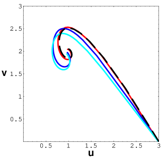
Figure 1: The $(u,v)$ curves for $y_{0}=100$ (red), $y_{0}=10$ (blue), and $y_{0}=6$ (cyan). The black dashed curve indicates the Newtonian isothermal sphere.

The behavior of curves near $(u,v)=(3,0)$ is found to be

$$u=3+bv\,\quad(v\ll 1)\,,$$ (29)

where

$$b=-\frac{3\left[\frac{3}{y_{0}}K_{1}(y_{0})+\left(1+\frac{12}{y_{0}^{2}}\right)K_{2}(y_{0})\right]}{5\left[K_{1}(y_{0})+\frac{3}{y_{0}}K_{2}(y_{0})\right]}\approx\left\{\begin{array}[]{ll}-\frac{3}{5}&(y_{0}\gg 1)\\ -\frac{12}{5y_{0}}&(y_{0}\ll 1)\end{array}\right.\,.$$ (30)

Figure 2 shows $b$ plotted against $y_{0}$.

Figure 2: Slope coefficient $b$ versus $y_{0}$.

Figure 3 shows the density profiles $\rho(x)/\rho_{c}$ as functions of $x\propto r$, where the curves in red, blue, and cyan correspond to the boundary conditions $y_{0}=100$, $10$, and $6$, respectively. In all of these cases, we find the asymptotic behavior $\rho\propto 1/r^{2}$, similarly to that of the Newtonian isothermal sphere which extends to infinity. Incidentally, it turns out that the asymptotics $v\approx 2$ read $y\approx 2\ln x$.

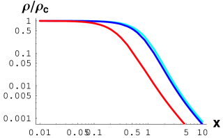
Figure 3: Density profiles $\rho(x)/\rho_{c}$ of general relativistic isothermal spheres for $y_{0}=100$ (red), $y_{0}=10$ (blue), and $y_{0}=6$ (cyan).

V.2 Isothermal spheres in Hořava gravity

Next, we consider the isothermal spheres in Hořava gravity.

The spirals of solutions in the $(u,v)$ plane are shown in Fig. 4. The fixed point $(u,v)\approx(1,2)$ is almost unchanged.

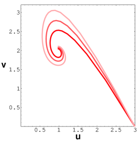
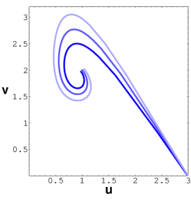
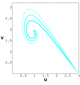
(a)                                             (b)                                             (c)

Figure 4: Plots of spirals in the $(u,v)$ plane. (a) $y_{0}=100$, (b) $y_{0}=10$, and (c) $y_{0}=6$. From the inner spiral to the outer spiral, $\alpha=0$, $\alpha=0.5$, and $\alpha=1$ in each plot.

Near the starting point, $(u,v)=(3,0)$, the curve is approximated as

$$u=3+bv\,\quad(v\ll 1)\,,$$ (31)

where

$$b=-\frac{3\left(1+\frac{2\alpha}{3}+\sqrt{1+\frac{2\alpha}{3}}\right)}{10\left(1+\frac{2\alpha}{3}\right)}\frac{\frac{3}{y_{0}}K_{1}(y_{0})+\left(1+\frac{12}{y_{0}^{2}}\right)K_{2}(y_{0})}{K_{1}(y_{0})+\frac{3}{y_{0}}K_{2}(y_{0})}\approx\left\{\begin{array}[]{ll}-\frac{3\left(1+\frac{2\alpha}{3}+\sqrt{1+\frac{2\alpha}{3}}\right)}{10\left(1+\frac{2\alpha}{3}\right)}&(y_{0}\gg 1)\\ -\frac{6\left(1+\frac{2\alpha}{3}+\sqrt{1+\frac{2\alpha}{3}}\right)}{5\left(1+\frac{2\alpha}{3}\right)y_{0}}&(y_{0}\ll 1)\,.\end{array}\right.$$ (32)

Thus, the spirals become larger according to the increase in the value of $\alpha$. The curves in the low-density case with $y_{0}=100$ are given in Fig. 4(a). The relatively high-density cases with $y_{0}=10$ [Fig. 4(b)] and $y_{0}=6$ [Fig. 4(c)] exhibit similar characteristics. The coefficient $b$ is plotted against $\alpha$ and $y_{0}$ in Fig. 5.

Figure 5: Slope coefficient $b$ plotted against $\alpha$ and $y_{0}$.

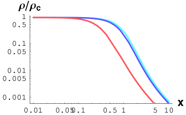
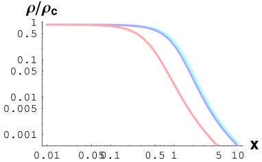
(a)                                                              (b)

Figure 6: The density profiles $\rho(x)/\rho_{c}$ for $y_{0}=100$ (red), $y_{0}=10$ (blue), and $y_{0}=6$ (cyan) with the parameter $\alpha=0.5$ are plotted in (a) while those with $\alpha=1$ are plotted in (b).

The profiles of the energy density for $\alpha=0.5$ and $1$ are shown in Fig. 6. Note that here $\rho$ is defined by $\propto\frac{1}{4\pi r^{2}}\frac{dM(r)}{dr}$. They seem to have behaviors similar to the case in general relativity ($\alpha=0$). This is because the terms with the coefficient $\alpha$ in the equations are proportional to $M/r^{3}$, which behaves asymptotically $\propto 1/r^{2}$ for $r\rightarrow\infty$. In other words, all isothermal spheres in our present model have an outer region which is well described by the structure of the Newtonian isothermal spheres.

V.3 Stability

While the behaviors of the spirals in the $(u,v)$ plane and the density profiles have moderate dependence on the central density and the parameter $\alpha$ which appears in Hořava gravity, the parameter dependence of stability is very complicated as we will show below. Therefore, in the present paper, we only discuss the stability by considering the ratio of the sum of the mass of constituent particles and the mass of the isothermal sphere in the region of the fixed radius. The analyses using various known methods are left for future studies.

Because the isothermal spheres in our model have the same asymptotic density profile as the Newtonian one, we consider the finite spherical box to define the mass of the object Chandra ; BT ; Antonov ; LW ; Padmanabhan ; Chavanis2 ; Chavanis3 . We consider the region inside the sphere with radius $r$.

Here, we consider the ratio $mN_{p}/M$, where

$$N_{p}=4\pi\int_{0}^{r}n_{p}(r)\frac{r^{2}}{\sqrt{1-\frac{2GM(r)}{r}}}dr=\frac{1}{G\sqrt{4\pi G\rho_{c}}}\int_{0}^{x}\frac{y_{0}K_{2}(y(x^{\prime}))}{y(x^{\prime})[(K_{1}(y_{0})+\frac{3}{y_{0}}K_{2}(y_{0})]}\frac{{x^{\prime}}^{2}}{\sqrt{1-\frac{2\tilde{M}(x^{\prime})}{x^{\prime}}}}dx^{\prime}\,.$$ (33)

Then, the ratio can be expressed as

$$\frac{mN_{p}}{M}=\frac{1}{\tilde{M}(x)}\int_{0}^{x}\frac{y_{0}K_{2}(y(x^{\prime}))}{y(x^{\prime})[(K_{1}(y_{0})+\frac{3}{y_{0}}K_{2}(y_{0})]}\frac{{x^{\prime}}^{2}}{\sqrt{1-\frac{2\tilde{M}(x^{\prime})}{x^{\prime}}}}dx^{\prime}\,.$$ (34)

Figure 7 shows the ratio $mN_{p}/M$ versus $-\log_{10}[\rho/\rho_{c}]$. Since the ratio $\rho(r)/\rho_{c}$ monotonically decreases with $r$, as we have seen in this section, the radius of the spherical box becomes larger from left to right in the horizontal axis. Notice that, apart from some exceptions, the characteristic feature of the plots lies inside the finite region by selecting the scale of the axis.

Since $N_{p}=\int n_{p}\sqrt{\tilde{g}}d^{3}x$, the ratio $mN_{p}/M>1$ implies positive binding energy $mN_{p}-M$, so the isothermal sphere is expected to be energetically stable in this case.

We should also consider the maximum point of the ratio. On the right-hand side of the maximum, the increase of the radius of the sphere reduces the amount of binding energy per mass. Thus, there is a possibility that some smaller bodies produced by fission will be more stable than a single body.

In Fig. 7(a), we show the general relativistic case $(\alpha=0)$. If the central density is sufficiently large (i.e., the gas is rather relativistic in the vicinity of the center), the stable configuration disappears according to the above-mentioned criteria. Its critical value is $y_{0}\approx 7.8$. However, the change of the curve is complicated for $y_{0}>10$. For $y_{0}=100$, the maximum is located around $-\log_{10}[\rho(r)/\rho_{c}]\approx 2.5$. This is consistent with the known stability criterion for the Newtonian isothermal sphere $-\log_{10}[\rho(r)/\rho_{c}]<2.85$ Antonov ; LW ; Padmanabhan ; Chavanis2 ; Chavanis3 .

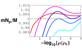
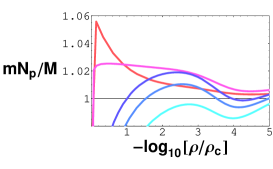
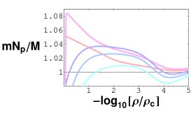
(a)                                             (b)                                             (c)

Figure 7: The ratio $mN_{p}/M$ is plotted. (a) $\alpha=0$, (b) $\alpha=0.5$, and (c) $\alpha=1$. In each plot, the red curve represents $y_{0}=100$, the magenta curve is for $y_{0}=30$, the blue curve is for $y_{0}=10$, the pale blue curve is for $y_{0}=7.8$, and the cyan curve is for $y_{0}=6$.

The Hořava-type gravity case is more complicated. The behaviors of the curves in Figs. 7(b) (for $\alpha=0.5$) and 7(c) (for $\alpha=1$) drastically change if $y_{0}$ is larger than about $10$. This is because the terms including $\alpha$ in (24) and (25), which have finite values in the central region [i.e., $\tilde{M}(x)/x^{3}=\frac{2}{3+\sqrt{9+6\alpha}}+O(x^{2})$ if $x\ll 1$], are dominant over the contribution of densities in the right-hand side of the equations in the small scale. Thus, the almost nonrelativistic gas sphere is stable when the radius is relatively small. Another important feature one can observe in Fig. 7 is that even the relatively high-central-density spheres may possess a stable radius if $\alpha$ is sufficiently large.

VI Conclusion

In this paper, we investigated isothermal spheres in general relativity and in a concise version of the Hořava gravity model. We concentrated on spherically symmetric and static solutions of the equations for the local equilibrium configuration. We found that the nonrelativistic limit reproduces the already-known Newtonian isothermal sphere.

We found that with Einstein gravity the stability of the sphere tends to be spoiled by the high density at the center of the general relativistic isothermal sphere. In Hořava-type gravity, the higher-derivative term stabilizes the sphere even if the central density is rather high; however, at the same time, the term makes the radius of the stable sphere very small with low central density.

In vacuum, the value of the parameter of Hořava gravity is severely limited observationally HKL . However, recalling that the parameter $\alpha$ is defined as $4\pi G\rho_{c}\frac{2}{\omega}$, it can be found that the value of $\alpha$ is generally enhanced in matter. Thus, it is meaningful to consider the higher-derivative correction in the study of the general high-density stellar structure. Studying various modified gravitational theories and other choices of equations of state is a good direction for future work. We will also continue discussing the stability from various points of view, including thermodynamical aspects, and we shall report such analyses in a future work.

Last but not least, we approached finite-temperature self-gravitating system from first principles. As a future task, the analyses of thermodynamical fluctuations with metric fluctuations should be studied carefully for investigating thermodynamical quantities in the system. A further theoretical study, including an extension to nonextensive statistical dynamics TS1 ; TS2 ; TS3 ; Chavanis4 ; Chavanis5 and generalization of canonically formulated gravity MN ; AFMNOP ; YOGM , will be reported elsewhere.

- (1) S. Chandrasekhar, Introduction to the study of stellar structure (Dover, New York, 1939).
- (2) J. Binney and S. Tremaine, Galactic Dynamics (Princeton Univ. Press, Princeton, 1987).
- (3) V. A. Antonov, “Most probable phase transition in spherical star systems and conditions for its existence”, Vest. Leningrad Univ. 7 (1962) 135; IAU Symposia 113 (1985) 525.
- (4) D. Lynden-Bell and R. Wood, “The gravo-thermal catastrophe in isothermal spheres and the onset of red-giant structure for stellar systems”, Mon. Not. R. Astron. Soc. 138 (1968) 495.
- (5) T. Padmanabhan, “Statistical mechanics of gravitating systems”, Phys. Rep. 188 (1990) 285.
- (6) P. H. Chavanis, “Gravitational instability of finite isothermal spheres”, A&A 381 (2002) 340.
- (7) C. Sire and P. H. Chavanis, “Thermodynamics and collapse of self-gravitating Brownian particles in dimensions”, Phys. Rev. E66 (2002) 046133.
- (8) G. Bertone, D. Hooper and J. Silk, “Particle dark matter: Evidence, candidates and constraints”, Phys. Rep. 405 (2005) 279.
- (9) S. Profumo, An Introduction to Particle Dark Matter (World Scientific, Singapore, 2017).
- (10) T. Clifton, P. G. Ferreira, A. Padilla and C. Skordis, “Modified Gravity and Cosmology”, Phys. Rep. 513 (2012) 1.
- (11) S. Capozziello and M. De Laurentis, “Extended Theories of Gravity”, Phys. Rep. 509 (2011) 167.
- (12) P. Hořava, “Membrane at quantum criticality”, JHEP 0903 (2009) 020.
- (13) P. Hořava, “Quantum gravity at a Lifshitz point”, Phys. Rev. D79 (2009) 084008.
- (14) G. Alberti and P. H. Chavanis, “Caloric curves of classical self-gravitating systems in general relativity”, Phys. Rev. E101 (2020) 052105.
- (15) W. C. Saslaw, S. D. Maharaj and N. Dadhich, “An isothermal universe”, ApJ 471 (1996) 571.
- (16) N. Dadhich, “Isothermal spherical perfect fluid model: Uniqueness and conformal mapping”, Pramana 49 (1997) 417.
- (17) N. Dadhich, “A conformal mapping and isothermal perfect fluid model”, Gen. Rel. Grav. 28 (1996) 1455.
- (18) N. Dadhich, S. Hansraj and S. D. Maharaj, “Universality of isothermal perfect fluid spheres in Lovelock gravity”, Phys. Rev. D93 (2016) 044072.
- (19) G. J. Olmo, D. Rubiera-Garcia and A. Wojnar, “Stellar structure models in modified theories of gravity: Lessons and Challenges”, Phys. Rep. 876 (2020) 1.
- (20) J. Sommer-Larsen, H. Vedel and U. Hellsten, “The structure of isothermal, self-gravitating, stationary gas spheres for softened gravity”, ApJ 500 (1998) 610.
- (21) A. Giusti, “MOND-like fractional Laplacian theory”, Phys. Rev. D101 (2020) 124029.
- (22) A. Giusti, R. Garrappa and G. Vachon, “On the Kuzmin model in fractional Newtonian gravity”, Eur. Phys. J. Plus 135 (2020) 798.
- (23) G. U. Varieschi, “Newtonian fractional-dimension gravity and MOND”, Found. Phys. 50 (2020) 1608.
- (24) G. U. Varieschi, “Newtonian fractional-dimension gravity and disk galaxies”, Eur. Phys. J. Plus 136 (2021) 183.
- (25) G. U. Varieschi, “Newtonian fractional-dimension gravity and rotationally supported galaxies”, Mon. Not. R. Astron. Soc. 503 (2021) 1915.
- (26) Z. F. Seidov, “Non- Newtonian gravitation and stellar structure”, astro-ph/9907136.
- (27) M. Lazar, “Gradient modification of Newtonian gravity”, Phys. Rev. D102 (2020) 096002.
- (28) A. Wang, “Horava gravity at a Lifshitz point: a progress report”, Int. J. Mod. Phys. D26 (2017) 1730014.
- (29) S. Nojiri and S. D. Odintsov, “Unified cosmic history in modified gravity: From theory to Lorentz non-invariant models”, Phys. Rep. 505 (2011) 59.
- (30) G. Cognola, R. Myrzakulov, L. Sebastiani, S. Vagnozzi and S. Zerbini, “Covariant Hořava-like and mimetic Horndeski gravity: cosmological solutions and perturbations”, Class. Quant. Grav. 33 (2016) 225014.
- (31) Y. S. Myung, Y.-W. Kim, W.-S. Son and Y.-J. Park, “Chaotic universe in the Hořava–Lifshitz gravity”, Phys. Rev. D82 (2010) 043506.
- (32) Y. S. Myung, “Chiral gravitational waves from Hořava–Lifshitz gravity”, Phys. Lett. B684 (2010) 1.
- (33) A. Kehagias and K. Sfetsos, “The black hole and FRW geometries of non-relativistic gravity”, Phys. Lett. B678 (2009) 123.
- (34) R. L. Arnowitt, S. Deser and C. W. Misner, “Canonical variables for general relativity”, Phys. Rev. 117 (1960) 1595. Gen. Rel. Grav. 40 (2008) 1997.
- (35) W. Greiner, L. Neise and H. Stöcker, “Thermodynamics and statistical mechanics” (Springer-Verlag, New York, 1995).
- (36) R. C. Tolman, Relativity, thermodynamics, and cosmology (Dover, New York, 1987).
- (37) T. Harko, Z. Kovács and F. S. N. Lobo, “Solar system tests of Hořava–Lifshitz gravity” Proc. R. Soc. A467 (2011) 1390.
- (38) A. Taruya and M. Sakagami, “Gravothermal catastorophe and Tsallis’ generalized entropy of self-gravitating systems”, Physica A307 (2002) 185.
- (39) A. Taruya and M. Sakagami, “Gravothermal catastorophe and Tsallis’ generalized entropy of self-gravitating systems. (II). Thermodynamic properties of stellar polytrope”, Physica A318 (2003) 387.
- (40) A. Taruya and M. Sakagami, “Gravothermal catastorophe and Tsallis’ generalized entropy of self-gravitating systems. (III). Quasi-equilibrium structure using normalized -values”, Physica A322 (2003) 285.
- (41) P. H. Chavanis, “Gravitational instability of polytropic spheres and generalized thermodynamics”, A&A 386 (2002) 732.
- (42) P. H. Chavanis and C. Sire, “Anomalous diffusion and collapse of self-gravitating Langevin particles in dimensions”, Phys. Rev. E69 (2004) 016116.
- (43) S. Mukohyama and K. Noui, “Minimally modified gravity: a Hamiltonian construction”, JCAP 1907 (2019) 049.
- (44) K. Aoki, A. De Felice, S. Mukohyama, K. Noui, M. Oliosi and M. C. Pookkillath, “Minimally modified gravity fitting Planck data better than CDM”, Eur. Phys. J. 80 (2020) 708.
- (45) Z.-B. Yao, M. Oliosi, X. Gao and S. Mukohyama, “Minimally modified gravity with an auxiliary constraint: a Hamiltonian construction”, Phys. Rev. D103 (2021) 024032.