Lowering Helstrom Bound with non-standard coherent states

Abstract.

In quantum information processing, using a receiver device to differentiate between two nonorthogonal states leads to a quantum error probability. The minimum possible error is known as the Helstrom bound. In this work we study and compare quantum limits for states which generalize the Glauber-Sudarshan coherent states, like non-linear, Perelomov, Barut-Girardello, and (modified) Susskind-Glogower coherent states. For some of these, we show that the Helstrom bound can be significantly lowered and even vanish in specific regimes.

1. Introduction

In quantum information processing, quantum operations represent communication channels while quantum states are the information carriers. The sender encodes information into a state $\rho$ which pertains to an alphabet $\mathcal{A}=\{\rho_{0},\rho_{1},\dotsc,\rho_{M}\}$. To find out which state was sent, the receiver carries out a measurement. When the transmitted states are not orthogonal, errors are possible and a nonzero probability exists that the receiver misconstrues the transmitted information (see [Holevo 1973] [Peres 1995] [Fuchs 1996] [Holevo 2011] and references therein). Note that the impossibility of differentiating between nonorthogonal states represents an advantage when dealing with quantum key distribution [Bennet&Brassard 1984]. In fact, using a nonorthogonal alphabet implies that any measurement disturbs the state and thus allows to impede an eavesdropper from obtaining information without being noticed. Moreover, as shown by Fuchs [Fuchs 1996], in some setups, nonorthogonality actually maximizes the classical information capacity in noisy channels.

In order to differentiate between nonorthogonal states one can optimize a state-determining measure over all POVMs, or positive operator valued measures. In [Holevo 1973], the author gives a systematic treatment of quantum statistical decision theory based on POVM. Necessary and sufficient conditions are given for optimality. Moreover the notion of maximum-likelihood measurement is introduced.

When trying to minimize the error in measurement over all possible POVM’s we are led to the quantum error probability, also known as Helstrom bound [Helstrom 1976]. This limit leads to a criterium of quality when discriminating between the transmitted nonorthogonal states.

For an on-off keyed alphabet (the pair formed by the Fock vacuum and an arbitrary coherent state) where the state discrimination is based on direct photon-counting, a discrimination error can occur when no photons are detected due to vacuum fluctuations. The discrimination error probability in this case is called the shot-noise-error probability (sometimes called standard quantum limit), it is always higher than the Helstron bound and is inversely proportional to the exponential of the average number of photons. Surpassing the shot noise in order to achieve the Hesltrom bound is an important subject of study in numerous works related to optical coherent state discrimination [Cook et al 2007, Tsujino et al 2011, Becerra et al 2013, Kunz et al 2019, Sych & Leuchs 2016, DiMario et al 2019].

A series of experimental and theoretical works using standard CS, i.e., Glauber-Sudarshan coherent states (or GS-CS) as nonorthogonal states were published, see [Cook et al 2007, Gazeau 2009] and references therein, for instance. On the one hand, GS-CS describe ideal lasers, on the other hand exhibit important mathematical properties. These are eigenstates of the annihilation operator in Fock Hilbert space and yield a Poissonian number distribution. In fact, real lasers are known to be better represented by states which are almost or non-Poissonian distributions [Perina 1984, Perina 1994]. Deviation from Poissonian statistics is also a consequence of non-linear effects in photons production. It is therefore important to study the mathematical and physical properties of “generalized” coherent states that exhibit both coherent and nonlinear behaviours. We should also mention recent results showing how using non-standard CS greatly enhances sensitivities of gravitational waves detectors, for both LIGO [Tse et al 2019] and VIRGO [Acernese et al 2019].

The present study concerns a class of non standard coherent states (the so-called “AN-CS”) which was introduced in [Gazeau 2019] and which encompasses most of the known generalisations of the Glauber-Sudarshan CS. They are denoted by $|\alpha;\boldsymbol{\mathsf{h}}\rangle$. We explore some of their statistical properties in terms of photon detection and examine if it is possible to lower the Helstrom bound in comparison with the GS-CS. This program was initiated by two of us in the article [Curado et al 2010], and we intend to pursue it with the present work. We have judged sufficient to restrict our study to the simplest case of the overlap $|\langle\alpha;\boldsymbol{\mathsf{h}}|0\rangle|$ with the vacuum, since the GS-CS’s themselves exhibit the well-known property $|\langle\alpha|\alpha^{\prime}\rangle|=|\langle\alpha-\alpha^{\prime}|0\rangle|$. We show that several non standard CS do indeed allow to decrease and even vanish the Helstrom limit in some regimes (for a given mean photons number), and this is the main outcome of our study.

In Section 2 we give a short overview of the Helstrom bound in binary communication based on POVM quantum measurement, and its value when we deal with GS-CS in the cases of perfect and imperfect detection. In Section 3 we recall the definition of the above mentioned AN-CS class of non standard coherent states [Gazeau 2019] and their most relevant statistical features, particularly in terms of the Mandel parameter, needed for implementing the present study devoted to the Helstrom bound. In Section 4 we examine the Helstrom bound for binary communication involving the vacuum and an arbitrary state in the AN-CS class, for both perfect and imperfect detections. In Section 5 we apply the above formalism to the so-called non-linear coherent states, a particular set of AN-CS. We examine in Section 6 the cases of SU$(2)$ and SU$(1,1)$ coherent states viewed as optical CS and unveil unexpected aspects of these states within the framework of quantum optics. In particular, we consider as quite appealing from a physical point of view our interpretation of SU$(2)$, i.e., spin, coherent states as a natural approximation of the Glauber-Sudarshan CS when the length of the beam is finite, which is actually always the case. We proceed in Section 7 with a similar study for non-linear CS built from deformed binomial distributions introduced in a series of works by two of us [Curado et al 2012, Bergeron et al 2012, Bergeron et al 2013]. Section 8 is devoted to the study of the Susskind-Glogower CS (see [Moya-Cessa and Soto-Eguibar 2011] and references therein) and a modified version that we introduce in this paper. We then conclude in Section 9 with a discussion about experimental and further theoretical possibilities offered by our results.

2. Hestrom Bound in binary communication

2.1. Definition

Let us consider a sender using nonorthogonal states as codewords, while the receiver executes a quantum measurement, $M$, on the channel in order to find out which state was sent. The measurement $M$ is set through a POVM defined by a complete (i.e., countable) set of positive operators [Peres 1995] that do resolve the identity,

(2.1) $$\sum_{i}M_{i}=\mathbb{1}\,\quad M_{i}\geq 0\,,$$

where $i$ stands for all possible outcomes.

Dealing with binary communication, there are two quantum measurement, $M_{0},M_{1}$ and the POVM resolution of unity then reads $M_{0}+M_{1}=\mathbb{1}$. The receiver can choose among two hypotheses: i) the transmitted state is $\rho_{0}$ for when the measurement outcome correlates with $M_{0}$, ii) the transmitted state is $\rho_{1}$, if the outcome corresponds to $M_{1}$.

An error might occur when there is a possibility for the receiver to measure one state while the sender actually had sent the other state. With binary communication there are two possible errors, these go with the following conditional probabilities:

(2.2) $$p(M_{0}|\rho_{1})=\mathrm{tr}[M_{0}\rho_{1}]=\mathrm{tr}[(I-M_{1})\rho_{1}]\,,\quad p(M_{1}|\rho_{0})=\mathrm{tr}[M_{1}\rho_{0}]\,.$$

Now, the total error probability reads

(2.3) $$p[M_{0},M_{1}]=\xi_{0}p({M}_{1}|\rho_{0})+\xi_{1}p({M}_{0}|\rho_{1})\,,\quad\xi_{0}+\xi_{1}=1\,,$$

with $\xi_{0}=p(\rho_{0})$ and $\xi_{1}=p(\rho_{1})$ standing for the classical probabilities that the sender might send $\rho_{0}$ and $\rho_{1}$, respectively; they encode the prior knowledge of the receiver about the sender chosen states. In many cases one uses $\xi_{0}=\xi_{1}=1/2$.

Minimizing the receiver measurement error over $M_{0}$ and $M_{1}$ yields the Helstrom bound, or quantum error probability,

(2.4) $$P_{\mathrm{H}}\equiv\min_{M_{0},M_{1}}p[M_{0},M_{1}]\,.$$

This is the smallest physically permitted error probability, given that the states $\rho_{0}$ and $\rho_{1}$ overlap.

Using pure states, $\rho_{0}=|\Psi_{0}\rangle\langle\Psi_{0}|$ and $\rho_{1}=|\Psi_{1}\rangle\langle\Psi_{1}|$, the Helstrom bound can be written as,

(2.5) $$P_{\mathrm{H}}=\frac{1}{2}\left(1-\sqrt{1-4\xi_{0}\xi_{1}|\langle\Psi_{1}|\Psi_{0}\rangle|^{2}}\right)\,.$$

The details can be found in [Gazeau 2019], for instance. Notice that, as would be expected, the quantum error vanishes for orthogonal states, i.e., $\langle\Psi_{1}|\Psi_{0}\rangle=0$.

2.2. Helstrom Bound with Glauber-Sudarshan Coherent States

2.2.1. Perfect detection

Light beams can be used as carriers of information in quantum communication. The Glauber-Sudarshan Coherent States (GS-CS) (also called linear or standard) are defined as the superposition of photon number states $|n\rangle$ given by

(2.6) $$|\alpha\rangle:=e^{-\frac{|\alpha|^{2}}{2}}\sum_{n=0}^{\infty}\frac{\alpha^{n}}{\sqrt{n!}}\left|n\right\rangle,\quad\text{where}\,\,\alpha\in\mathbb{C}\,.$$

They overlap as

(2.7) $$\langle\alpha|\alpha^{\prime}\rangle:=e^{-\frac{|\alpha|^{2}}{2}-\frac{|\alpha^{\prime}|^{2}}{2}+\bar{\alpha}\alpha^{\prime}}=e^{\mathsf{i}\mathrm{Im}\left(\bar{\alpha}\alpha^{\prime}\right)}e^{-\frac{|\alpha-\alpha^{\prime}|^{2}}{2}}\,.$$

For an alphabet of two GS-CS given by

(2.8) $$\rho=|\alpha\rangle\langle\alpha|\,,\quad\rho^{\prime}=|\alpha^{\prime}\rangle\langle\alpha^{\prime}|\,,$$

we have from (2.7)

(2.9) $$\mathrm{tr}\left(\rho\rho^{\prime}\right)=\left|\langle\alpha|\alpha^{\prime}\rangle\right|^{2}=e^{-|\alpha-\alpha^{\prime}|^{2}}=|\langle\alpha-\alpha^{\prime}|0\rangle|^{2}\,.$$

As was pointed out in the introduction, this property of the GS-CS allows to restrict our study to an alphabet of two GS-CS given by

(2.10) $$\rho_{0}=|0\rangle\langle 0|\,,\quad\rho_{1}=|\alpha\rangle\langle\alpha|\,,$$

for which

(2.11) $$\left|\langle\alpha|0\rangle\right|^{2}=e^{-|\alpha|^{2}}\,.$$

Now the quantity $u=|\alpha|^{2}$ is precisely the average value of the number operator $\hat{N}=\sum_{n=0}^{\infty}n|n\rangle\langle n|$, i.e. the mean value of number of photons in the CS $|\alpha\rangle$,

(2.12) $$\bar{n}=\langle\alpha|\hat{N}|\alpha\rangle=\sum_{n=0}^{\infty}n\frac{u^{n}e^{-u}}{n!}=u\,.$$

Note that $u$ can also be viewed as the mean value of the random variable $n$ with the Poissonian probability distribution

(2.13) $$\bar{n}=\sum_{n=0}^{\infty}n\mathsf{P}_{n}(u)\,\qquad\mathsf{P}_{n}(u)=\left|\langle\alpha|n\rangle\right|^{2}=e^{-u}\frac{u^{n}}{n!}.$$

Hence (2.11) becomes

(2.14) $$\left|\langle\alpha|0\rangle\right|^{2}=e^{-\bar{n}}\,,$$

and the quantum error probability reads in this case

(2.15) $$P_{\mathrm{H}}=\frac{1}{2}\left(1-\sqrt{1-4\xi_{0}\xi_{1}e^{-\bar{n}}}\right)\equiv P_{\mathrm{H}}(\bar{n})\,.$$

2.2.2. Imperfect detection

In practice, only a fraction $\eta$ of the photons reaching a photo-counter leads to a count. The parameter $\eta\in[0,1]$ is called the efficiency parameter. For imperfect detection ($\eta<1$), the binomial distribution allows to compute the probability $\mathsf{P}_{n}(u;\eta)$ to detect $n$-photons as a function of $\eta$. Sub-unity photodetector efficiency yields a photon-count which is linked to the perfect ($\eta=1$) photon distribution $\mathsf{P}_{m}(u)=\mathsf{P}_{m}(u;\eta=1)$ through a Bernoulli transformation [Loudon 1973]:

(2.16) $$\mathsf{P}_{n}(u;\eta)=\sum_{m=n}^{\infty}\binom{m}{n}{\eta^{n}}\,(1-\eta)^{m-n}\,\mathsf{P}_{m}(u;\eta=1).$$

The GS-CS’s exhibit the useful property that non-unit quantum efficiency corresponds to a perfect detector equipped with a beam-splitter having a transmission coefficient $\eta\leq 1$. In fact, since one has the Poisson distribution for GS coherent states and an ideal detector, (2.13), replacing $m$ by $s=m-n$ in the summation (2.16) leads to

(2.17) $$\mathsf{P}_{n}(u;\eta)=\frac{\eta^{n}u^{n}}{n!}\,e^{-\eta u}=\frac{(\eta u)^{n}}{n!}\,e^{-\eta u}=\mathsf{P}_{n}(\eta u)\,.$$

In other words, one can “hide” the imperfection of the detector into an effective state by changing

(2.18) $$\alpha\to\sqrt{\eta}\alpha.$$

This amounts to replace the previous setup based on the alphabet $\{|0\rangle,|\alpha\rangle\}$ and an imperfect detector ($\eta<1$) with a new one based on $\{|0\rangle,|\sqrt{\eta}\alpha\rangle\}$ and a perfect detector [Geremia 2004]. Then, the overlap of the new alphabet reads

(2.19) $$\left|\langle\sqrt{\eta}\alpha|0\rangle\right|^{2}=e^{-\eta\bar{n}}\,,$$

where $\eta\bar{n}$ is equal to the mean photon number given by the modified probability distribution (2.17).

(2.20) $$\bar{n}_{\eta}=\sum_{n=0}^{\infty}n\,\mathsf{P}_{n}(u;\eta)=\eta u=\eta\bar{n}\,.$$

This allows to write down the Helstrom bound (2.5) for the imperfect case as

(2.21) $$P_{\mathrm{H}}(\bar{n};\eta)=\frac{1}{2}\left(1-\sqrt{1-4\xi_{0}\xi_{1}e^{-\bar{n}_{\eta}}}\right)\,.$$

This indicates that there is always a non-zero quantum error probability with GS-CS.

3. A class of non standard coherent states in Quantum Optics: the AN-CS

Most of the generalisations of GS-CS encountered in quantum optics or quantum mechanics are coherent states in the AN class (AN for “$\alpha n$”) [Gazeau 2019]. These “AN-CS” are one-mode Fock states of the form;

(3.1) $$|\alpha;\boldsymbol{\mathsf{h}}\rangle=\sum_{n=0}^{\infty}\alpha^{n}\,h_{n}(|\alpha|^{2})|n\rangle\,,$$

where the complex $\alpha$ lies in the open disk $\mathcal{D}_{R}$ of radius $R$, $|\alpha|<R$, with $R$ being finite or infinite. The sequence $\boldsymbol{\mathsf{h}}:=\left(h_{n}\right)\,,\,n=0,1,2,\dotsc$ of real-valued functions

(3.2) $$[0,R^{2})\ni u:=|\alpha|^{2}\mapsto h_{n}(u)$$

is requested to obey the three fundamental conditions:

(3.3) $$\sum_{n=0}^{\infty}u^{n}\,\left(h_{n}(u)\right)^{2}\,=1,\quad\mbox{(normalisation 1)}\,,$$

(3.4) $$[0,R^{2})\ni u\mapsto\bar{n}_{\boldsymbol{\mathsf{h}}}(u) :=\sum_{n=0}^{\infty}n\,u^{n}\,\left(h_{n}(u)\right)^{2}\quad\mbox{is strictly increasing}\,,$$

(3.5) $$\exists w:[0,R^{2}]\to{\mathbb{R}}^{+}\ \mbox{such that}\ \int_{0}^{R^{2}}\mathrm{d}u\,w(u)\,u^{n}\left(h_{n}(u)\right)^{2}\,=1,\quad\mbox{(normalisation 2)}\,,$$

where $w$ is a weight function.

Note that the GS-CS’s are the particular case

(3.6) $$h_{n}(u)=\frac{e^{-u/2}}{\sqrt{n!}}\,,\quad w(u)=1\,\,,\,\,\,\,\,\,R=\infty\,.$$

A finite summation in (3.1) due to $h_{n}=0$ for n larger than some $n_{\mathrm{max}}$ might be considered in the present study. In this case we consider as Hilbert space the finite dimensional Hilbert space spanned by the orthonormal basis ($\{|n\rangle\})_{n=0}^{n_{\mathrm{max}}}$. Spin CS’s in Subsection 6.1 are an illustration of this case.

In the infinite sum case, special conditions are to be imposed on the sequence of functions $h_{n}$ in order to insure the convergence of series (3.3) for all $0\leq u<R^{2}$ and integrals (3.5) for all $n$.

Condition Eq. (3.3) means that the vectors (3.1) are normalised states of a Fock Hilbert space formed by the number states. This yields a probability distribution on $\mathbb{N}$

(3.7) $$n\mapsto\mathsf{P}^{\boldsymbol{\mathsf{h}}}_{n}(u)=\left|\langle\alpha;\boldsymbol{\mathsf{h}}|n\rangle\right|^{2}=u^{n}\,\left(h_{n}\left(u\right)\right)^{2}$$

where $u$ is now a parameter. This is exactly the probability of registering $n$ photons with a measuring ideal device, i.e., having maximal efficiency ($\eta=1$) when the light beam is in the non standard coherent state $|\alpha;\boldsymbol{\mathsf{h}}\rangle$.

Condition Eq. (3.4) expresses that the expected value

(3.8) $$\langle\alpha;\boldsymbol{\mathsf{h}}|\hat{N}|\alpha;\boldsymbol{\mathsf{h}}\rangle=\sum_{n=0}^{+\infty}n\mathsf{P}^{\boldsymbol{\mathsf{h}}}_{n}(u)\equiv\bar{n}_{\boldsymbol{\mathsf{h}}}(u)$$

of the number operator in AN-CS is a one-to-one relation with $u$ and so can be inverted.

Condition Eq. (3.5) implies the resolution of the identity in the same Fock space:

(3.9) $$\int_{\mathcal{D}_{R}}\frac{\mathrm{d}^{2}\alpha}{\pi}\,w\left(|\alpha|^{2}\right)\,|\alpha;\boldsymbol{\mathsf{h}}\rangle\langle\alpha;\boldsymbol{\mathsf{h}}|=\mathbb{1}\,.$$

This property holds because of the orthonormality relations

(3.10) $$\int_{\mathcal{D}_{R}}\frac{\mathrm{d}^{2}\alpha}{\pi}\,w\left(|\alpha|^{2}\right)\,\bar{\alpha}^{n^{\prime}}\alpha^{n}h_{n^{\prime}}\left(|\alpha|^{2}\right)\,h_{n}\left(|\alpha|^{2}\right)=\delta_{nn^{\prime}}$$

stemming from Fourier angular integration on the argument of $\alpha$ and the kind of moment problem solved by (3.5). The latter allows us to interpret the map

(3.11) $$\alpha\mapsto\mathsf{P}^{\boldsymbol{\mathsf{h}}}_{n}\left(|\alpha|^{2}\right)$$

as an isotropic probability distribution, with parameter $n$, on the disk $\mathcal{D}_{R}$, equipped with the measure $w\left(|\alpha|^{2}\right)\,\dfrac{\mathrm{d}^{2}\alpha}{\pi}$. Equivalently, the map

(3.12) $$[0,R^{2})\ni u\mapsto\mathsf{P}^{\boldsymbol{\mathsf{h}}}_{n}(u)$$

is a probability distribution on the interval $[0,R^{2})$ equipped with the measure $w(u)\mathrm{d}u$.

The average value (3.8) of the number operator might be interpreted as the intensity (or energy if multiplied by $\hbar\omega$) of the quantum radiation (monochromatic) in the state $|\alpha;\boldsymbol{\mathsf{h}}\rangle$. Thus, an optical phase space related to this “AN-CS radiation” might be constructed through the map

(3.13) $$\mathcal{D}_{R}\ni\alpha\mapsto\zeta_{\alpha}=\sqrt{\bar{n}_{\boldsymbol{\mathsf{h}}}\left(|\alpha|^{2}\right)}\,e^{\mathsf{i}\arg\alpha}\in\mathbb{C}\,.$$

The fluctuations of the number of photons about its mean value are quantified in terms of the standard deviation

(3.14) $$\Delta n_{\boldsymbol{\mathsf{h}}}(u)=\sqrt{\overline{n^{2}_{\boldsymbol{\mathsf{h}}}}-\left(\bar{n}_{\boldsymbol{\mathsf{h}}}\right)^{2}}\,,\quad\overline{n^{2}_{\boldsymbol{\mathsf{h}}}}(u)=\sum_{n}n^{2}\mathsf{P}^{\boldsymbol{\mathsf{h}}}_{n}(u)\,.$$

The distribution $n\mapsto\mathsf{P}^{\boldsymbol{\mathsf{h}}}_{n}(u)$ is then classified as: sub-Poissonian for $\Delta n_{\boldsymbol{\mathsf{h}}}<\sqrt{\bar{n}_{\boldsymbol{\mathsf{h}}}}$, Poissonian for $\Delta n_{\boldsymbol{\mathsf{h}}}=\sqrt{\bar{n}_{\boldsymbol{\mathsf{h}}}}$ and super-Poissonian for $\Delta n_{\boldsymbol{\mathsf{h}}}>\sqrt{\bar{n}_{\boldsymbol{\mathsf{h}}}}$. The deviation of $\mathsf{P}^{\boldsymbol{\mathsf{h}}}_{n}(u)$ from the Poisson distribution, is conveniently measured with the Mandel parameter $Q^{\boldsymbol{\mathsf{h}}}_{M}$. The latter is defined as

(3.15) $$Q^{\boldsymbol{\mathsf{h}}}_{M}(u):=\frac{\overline{n^{2}_{\boldsymbol{\mathsf{h}}}}-\left(\bar{n}_{\boldsymbol{\mathsf{h}}}\right)^{2}}{\bar{n}_{\boldsymbol{\mathsf{h}}}}-1\,,$$

and it is clear to see that it should be larger than or equal $-1$. At a given $u$ the distribution $\mathsf{P}^{\boldsymbol{\mathsf{h}}}_{n}(u)$ is respectively Poissonian if $Q^{\boldsymbol{\mathsf{h}}}_{M}(u)=0$, sub-Poissonian if $Q^{\boldsymbol{\mathsf{h}}}_{M}(u)<0$, and super-Poissonian if $Q^{\boldsymbol{\mathsf{h}}}_{M}(u)>0$. Actually, due to the bijective relation between $u$ and $\bar{n}$ according to Assumption (3.4), we will preferably analyse the behaviour of the Mandel parameter in function of the physical $\bar{n}$:

(3.16) $$\widetilde{Q^{\boldsymbol{\mathsf{h}}}_{M}}(\bar{n})=Q^{\boldsymbol{\mathsf{h}}}_{M}(u(\bar{n}))\,.$$

4. Helstrom bound for states in the AN-class versus GS-CS

4.1. Perfect detection

The Helstrom bound (HB) for an alphabet composed of pure states depends only on the overlap between them, as it is obvious from (2.5). If one wishes to lower the HB in comparison with the HB 2.15 involving GS-CS, it is necessary to lower the overlap of the two involved states. For this reason we are interested in states with a non-Poissonian photon distribution. Since our objective is to compare their corresponding HB with (2.15) and (2.21), we restrict our study to the overlap between the vacuum and an arbitrary AN-CS. Accordingly, for an alphabet of two AN-CS’s given respectively by

(4.1) $$\rho_{0}=|0;\boldsymbol{\mathsf{h}}\rangle\langle 0;\boldsymbol{\mathsf{h}}|\,,\quad\rho_{1}=|\alpha;\boldsymbol{\mathsf{h}}\rangle\langle\alpha;\boldsymbol{\mathsf{h}}|\,,$$

the modulus squared of the overlap reads

(4.2) $$\left|\langle\alpha;\boldsymbol{\mathsf{h}}|0;\boldsymbol{\mathsf{h}}\rangle\right|^{2}=\left(h_{0}(u)\right)^{2}\,.$$

Then the corresponding HB reads,

(4.3) $$P^{\boldsymbol{\mathsf{h}}}_{\mathrm{H}}=\frac{1}{2}\left(1-\sqrt{1-4\xi_{0}\xi_{1}\left(h_{0}(u)\right)^{2}}\right).$$

Comparing two Helstrom bounds is physically meaningful only if one views them as a function of the average number of photons $\overline{n}$. This is made possible thanks to Condition (3.4) which allows us to express unambiguously the inverse function $\bar{n}\mapsto u^{\boldsymbol{\mathsf{h}}}(\bar{n})$ from Eq. (3.8). Hence, $P^{\boldsymbol{\mathsf{h}}}_{\mathrm{H}}$ in Eq. (4.3) can be written as a function of $\bar{n}$

(4.4) $$\bar{n}\mapsto P^{\boldsymbol{\mathsf{h}}}_{\mathrm{H}}(\bar{n})=\frac{1}{2}\left(1-\sqrt{1-4\xi_{0}\xi_{1}\left(h_{0}\left(u^{\boldsymbol{\mathsf{h}}}(\bar{n})\right)\right)^{2}}\right)\,.$$

Comparing this HB with the standard one given by (2.15) amounts to study the function

(4.5) $$\Delta^{\boldsymbol{\mathsf{h}}}(\bar{n}):=\left(h_{0}\left(u^{\boldsymbol{\mathsf{h}}}(\bar{n})\right)\right)^{2}-e^{-\bar{n}}\,.$$

Indeed, we have

(4.6) $$\Delta^{\boldsymbol{\mathsf{h}}}(\bar{n})\lesseqqgtr 0\Longleftrightarrow P^{\boldsymbol{\mathsf{h}}}_{\mathrm{H}}(\bar{n})\lesseqqgtr P_{\mathrm{H}}(\bar{n})\,.$$

4.2. Imperfect detection

In the case of imperfect detection, the probability $\mathsf{P}^{\boldsymbol{\mathsf{h}}}_{n}(u;\eta)$ to detect $n$-photons using a non-perfect detector ($\eta<1$) is given in terms of the (perfect detector) probability, $\mathsf{P}^{\boldsymbol{\mathsf{h}}}_{m}(u)=\mathsf{P}^{\boldsymbol{\mathsf{h}}}_{m}(u;\eta=1),$ through the Bernoulli transformation (2.16)

(4.7) $$\mathsf{P}^{\boldsymbol{\mathsf{h}}}_{n}(u;\eta)=\sum_{m=n}^{\infty}\binom{m}{n}\eta^{n}\,(1-\eta)^{m-n}\,\mathsf{P}^{\boldsymbol{\mathsf{h}}}_{m}(u;\eta=1)$$

This transformation has the following important property. The mean value of a function $n\mapsto\varphi(n)$ with respect to the above distribution is given by:

(4.8) $$\overline{\varphi(n)}(u;\eta)=\sum_{n=0}^{+\infty}\varphi(n)\,\mathsf{P}^{\boldsymbol{\mathsf{h}}}_{n}(u;\eta)=\sum_{n=0}^{+\infty}\langle\varphi\rangle_{n;\eta}\,\mathsf{P}^{\boldsymbol{\mathsf{h}}}_{n}(u;\eta=1)\,,$$

where $\langle\cdot\rangle_{n;\eta}$ is the mean value with respect to the binomial distribution with parameter $\eta$ and for $n$ trials,

(4.9) $$\langle\varphi\rangle_{n;\eta}=\sum_{k=0}^{n}\binom{n}{k}\eta^{k}\,(1-\eta)^{n-k}\,\varphi(k)\,.$$

For the number function, $\varphi(k)=k$, $\langle\varphi\rangle_{n;\eta}=\eta n$, and we end up with the simple expression

(4.10) $$\bar{n}(u;\eta)=\eta\bar{n}(u;\eta=1)\equiv\eta\bar{n}(u)\,.$$

There results that the only change we have to do in the expression (4.5) and the inequalities (4.6) is to replace $\bar{n}$ with $\eta\bar{n}$:

(4.11) $$\Delta^{\boldsymbol{\mathsf{h}}}(\eta\bar{n}):=\left(h_{0}\left(u^{\boldsymbol{\mathsf{h}}}(\eta\bar{n})\right)\right)^{2}-e^{-\eta\bar{n}}\,,$$

and

(4.12) $$\Delta^{\boldsymbol{\mathsf{h}}}(\eta\bar{n})\lesseqqgtr 0\Longleftrightarrow P^{\boldsymbol{\mathsf{h}}}_{\mathrm{H}}(\eta\bar{n})\lesseqqgtr P_{\mathrm{H}}(\eta\bar{n})\,.$$

It is clear from the above that the behavior of the Helstrom bound with regard to the GS-CS case is not $\eta$-dependent. Note that the relation (4.10) reduces to the rescaled $\alpha$ parameter (2.19) in the case of the standard GS-CS.

5. Helstrom bound with “non-linear” coherent states

We define non-linear CS (NL-CS) as AN-CS for with functions $h_{n}(u)$ assuming the deformed Poissonian form

(5.1) $$h_{n}(u)=\frac{\lambda_{n}}{\sqrt{\mathcal{N}(u)}}\equiv\frac{1}{\sqrt{\mathcal{N}(u)}}\,\frac{1}{\sqrt{x_{n}!}}\,,\quad x_{0}!:=1\,,\quad x_{n}!:=x_{1}x_{2}\cdots x_{n}\,,$$

where the $\lambda_{n}$’s form a strictly decreasing sequence of positive numbers,

(5.2) $$\boldsymbol{\lambda}:=(\lambda_{n})_{n\in\mathbb{N}}\,,\quad\lambda_{0}=1\,,$$

i.e., the $x_{n}$’s, $x_{n}:=\left(\frac{\lambda_{n-1}}{\lambda_{n}}\right)^{2}$, form the strictly increasing sequence

(5.3) $$\boldsymbol{\chi}:=(x_{n})_{n\in\mathbb{N}}\,,\quad 0=x_{0}<x_{1}<x_{2}\cdots x_{n}<x_{n+1}<\cdots\,.$$

The function $\mathcal{N}(u)$ is the generalized exponential with radius $R^{2}$,

(5.4) $$\mathcal{N}(u)=\sum_{n}\lambda_{n}^{2}u^{n}=\sum_{n}\frac{u^{n}}{x_{n}!}\,,$$

The corresponding NL-CS read

(5.5) $$|\alpha;\boldsymbol{\lambda}\rangle=|\alpha;\boldsymbol{\chi}\rangle=\frac{1}{\sqrt{\mathcal{N}\left(|\alpha|^{2}\right)}}\sum_{n}\lambda_{n}\alpha^{n}|n\rangle=\frac{1}{\sqrt{\mathcal{N}\left(|\alpha|^{2}\right)}}\sum_{n}\frac{\alpha^{n}}{\sqrt{x_{n}!}}|n\rangle\,.$$

Here, for the sake of simplicity, we drop subscript $\boldsymbol{\mathsf{h}}$ or $\boldsymbol{\lambda}$ or $\boldsymbol{\chi}$. The normalisation condition (3.5) is fulfilled if there exists a weight $w(u)$ solving the Stieltjes moment problem [Akhiezer 1965] for the sequence $(x_{n}!)_{n\in\mathbb{N}}$,

(5.6) $$x_{n}!=\int_{0}^{R^{2}}\mathrm{d}u\,\frac{w(u)}{\mathcal{N}(u)}\,u^{n}\,.$$

The detection probability follows the deformed Poisson distribution:

(5.7) $$n\mapsto\mathsf{P}_{n}(u)=\left|\langle\alpha;\boldsymbol{\chi}|n\rangle\right|^{2}=\frac{1}{\mathcal{N}(u)}\,\frac{u^{n}}{x_{n}!}\,.$$

The average value $\bar{n}$ of the number operator, as a function of $u=|\alpha|^{2}$, is given by

(5.8) $$\bar{n}(u)=\langle\alpha|\hat{N}|\alpha\rangle=u\frac{\mathcal{N}^{\prime}(u)}{\mathcal{N}(u)}=u\frac{\mathrm{d}\log\mathcal{N}(u)}{\mathrm{d}u}\,.$$

The above relation imposes that

(5.9) $$\mathcal{N}^{\prime}(u)>0\,,$$

i.e., $\mathcal{N}(u)$ is strictly increasing from $\mathcal{N}(0)=1$ over $\mathbb{R}_{+}$.

Now, Condition (3.4) imposes a further relation on nonlinear CS:

(5.10) $$\frac{\mathrm{d}\bar{n}}{\mathrm{d}u}=\left(\frac{d}{du}+u\,\frac{d^{2}}{du^{2}}\right)\ln\mathcal{N}(u)\,>0.$$

The expected value $\overline{n^{2}}$ is given by

(5.11) $$\overline{n^{2}}(u)=\frac{u}{\mathcal{N}(u)}\frac{\mathrm{d}}{\mathrm{d}u}u\frac{\mathrm{d}}{\mathrm{d}u}\mathcal{N}(u)\,,$$

and the Mandel parameter $Q_{M}(u)$ reads

(5.12) $$Q_{M}(u)=u\left(\frac{\mathcal{N}^{\prime\prime}(u)}{\mathcal{N}^{\prime}(u)}-\frac{\mathcal{N}^{\prime}(u)}{\mathcal{N}(u)}\right)=u\frac{\mathrm{d}}{\mathrm{d}u}\ln\left(\frac{\mathrm{d}}{\mathrm{d}u}\ln\mathcal{N}(u)\right)\,.$$

Let us put

(5.13) $$\mathcal{N}(u)=e^{F(u)}\,,\quad F(0)=0\,.$$

Since for $u>0$, $0<\mathcal{N}^{\prime}(u)=F^{\prime}(u)e^{F(u)}$, we have $F^{\prime}(u)>0$ for $u>0$, i.e. $F(u)$ is strictly increasing over $\mathbb{R}_{+}$ from $F(0)=0$. Note that $F^{\prime}(u)=\dfrac{\bar{n}(u)}{u}\,$. In term of $F$, the Mandel parameter assumes the simpler form:

(5.14) $$Q_{M}(u)=u\,\frac{F^{\prime\prime}(u)}{F^{\prime}(u)}=u\frac{\mathrm{d}}{\mathrm{d}u}\ln F^{\prime}(u)\,.$$

In this case, (5.10) leads to $u\,\dfrac{F^{\prime\prime}}{F^{\prime}}=u\,\dfrac{\mathrm{d}\ln F^{\prime}}{\mathrm{d}u}>-1\,$, which is consistent with the known lower bound on Mandel parameter. Hence, the NL-CS (5.5) are Poissonian if and only if $F^{\prime\prime}(u)=0$ for all $u\in\mathbb{R}_{+}$, i.e. if they are the GS-CS. They are sub-Poissonian (resp. super-Poissonian) at $u$ if $F^{\prime\prime}(u)<0$ (resp. $>0$).

Finally, applying the expression (4.5) to compare the Helstrom Bounds between the above NL-CS (5.5) and the GS-CS leads to

(5.15) $$P^{\chi}_{\mathrm{H}}(\bar{n})\lesseqqgtr P_{\mathrm{H}}(\bar{n})\Longleftrightarrow\Delta(\bar{n})=e^{-F(u(\bar{n}))}-e^{-\bar{n}}\lesseqqgtr 0\Longleftrightarrow\bar{n}\lesseqqgtr F(u(\bar{n}))\,.$$

6. Mandel Parameter and Helstrom Bound for selected NL-CS families

6.1. Spin CS as optical CS

This set of states derives from the Gilmore or Perelomov SU$(2)$-CS, also called spin CS [Perelomov 1972, Perelomov 1986], adapted to the context of quantum optics. The Fock space reduces to the finite-dimensional subspace $\mathcal{H}_{j}$, with dimension $n_{j}+1:=2j+1$, $j$ being a positive integer or half-integer. They are defined through (3.1) and (5.1) with

(6.1) $$h_{n}(u)=\lambda_{n}\,(1+u)^{-\frac{n_{j}}{2}}\,,\quad\lambda_{n}=\sqrt{\binom{n_{j}}{n}}\,,\quad\binom{n_{j}}{n}=\frac{n_{j}!}{n!(n_{j}-n)!}\,,\quad x_{n}=\frac{n}{n_{j}-n+1}\,,$$

for $n\in[0,n_{j}]$; $h_{n>n_{j}}(u)=0$. The corresponding generalised exponential is the binomial

(6.2) $$\mathcal{N}(u)=(1+u)^{n_{j}}\,,$$

and the related NL-CS read as

(6.3) $$|\alpha;n_{j}\rangle=\left(1+|\alpha|^{2}\right)^{-\frac{n_{j}}{2}}\sum_{n=0}^{n_{j}}\sqrt{\binom{n_{j}}{n}}\,\alpha^{n}\,|n\rangle\,.$$

They resolve the unity in $\mathcal{H}_{n_{j}}$ in the following way:

(6.4) $$\frac{n_{j}+1}{\pi}\,\int_{\mathbb{C}}\frac{\mathrm{d}^{2}\alpha}{(1+|\alpha|^{2})^{2}}\,|\alpha;n_{j}\rangle\langle\alpha;n_{j}|=\mathbb{1}\,.$$

The detection probability follows the binomial distribution:

(6.5) $$n\mapsto\mathsf{P}_{n}(u)=(1+u)^{-n_{j}}\,\binom{n_{j}}{n}\,u^{n}\,.$$

The number operator average value then reads

(6.6) $$\bar{n}(u)=n_{j}\,\frac{u}{1+u}\ \Leftrightarrow\ u=\frac{\bar{n}/n_{j}}{1-\bar{n}/n_{j}}\,,$$

which is depicted in Figure 1 for $n_{j}=4$ and $10$. The probability (6.5) is thus expressed in terms of $p:=\bar{n}/n_{j}$ as

(6.7) $$\mathsf{P}_{n}(u)\equiv\widetilde{\mathsf{P}}_{n}(p)=\binom{n_{j}}{n}\,(1-p)^{n_{j}-n}\,p^{n}\,.$$

As a consequence one can build an optical phase space as the open disk of radius $\sqrt{n_{j}}$,

$$\mathcal{D}_{\sqrt{n_{j}}}=\left\{\zeta_{\alpha}=\sqrt{\bar{n}\left(|\alpha|^{2}\right)}e^{\mathsf{i}\arg\alpha}\,,\,|\zeta_{\alpha}|<\sqrt{n_{j}}\right\}\,.$$

In terms of photon statistics, the physical interpretation of the binomial distribution together with $n_{j}$ is decidedly clear when considering a beam of light which is perfectly coherent and has constant intensity. For a beam of a finite length $L$ which is divided in $n_{j}$ parts of length $L/n_{j}$, $\widetilde{\mathsf{P}}_{n}(p)$ stands for the probability to find, in any possible order, one photon in $n$ segments and no photon in the remaining $(n_{j}-n)$ segments [Fox 2006]. A more general interpretation of the above distributions (6.5) and (6.7) can be found in [Ali et al 2008].

Note that the GS-CS derive from the above states in the limit $n_{j}\to\infty$. This goes throughout a contraction process which consists in rescaling the complex variable $\alpha$ through $\alpha\mapsto\sqrt{n_{j}}\,\alpha$. As a consequence the distribution $\widetilde{\mathsf{P}}_{n}(p)$ reduces to (2.13).

By applying (5.14) with $F(u)=n_{j}\ln(1+u)$, the expression of the Mandel parameter (as a function of $u$ or as a function of $\bar{n}$) is independent of $j$ and is given by

(6.8) $$Q_{M}(u)=-\frac{u}{1+u}\ \Leftrightarrow\ \widetilde{Q}_{M}(\bar{n})=-\frac{\bar{n}}{n_{j}}\,.$$

Hence, states (6.3) are always sub-Poissonian, as shown in Figure 1. This fundamentally quantum feature is easily understood since they are built from a finite number of photons.

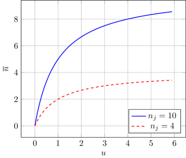
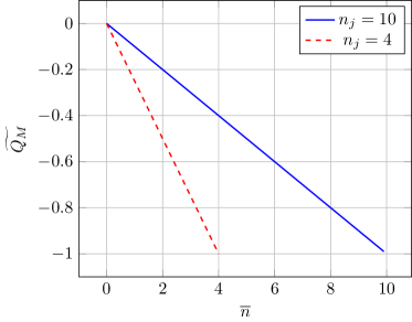
Figure 1. Photon statistics for optical spin CS (6.3) with $n_{j}=4$ and $10$. These states are always sub-Poissonian. Left figure: Average value of photons as a function of $u$. Right figure: Mandel parameter $\widetilde{Q_{M}}$ (6.8) as a function of $\bar{n}$.

Concerning the Helstrom bound, we examine the expression (4.5) in the present case:

(6.9) $$\Delta(\bar{n})=\left(1-\frac{\bar{n}}{n_{j}}\right)^{n_{j}}-e^{-\bar{n}}\,.$$

From the Bernouilli-like inequality

(6.10) $$(1+x)^{r}\leq e^{rx}\,,$$

valid for any $r>0$ and any real $x$, we infer that $\Delta(\bar{n})\leq 0$ for any $\bar{n}$ and $j$. Hence the spin CS Helstrom bound is lower than the GS-CS Helstrom bound for any value of $u=|\alpha|^{2}$, see Figure 2. This is a remarkable result which confirms their deep quantum nature.

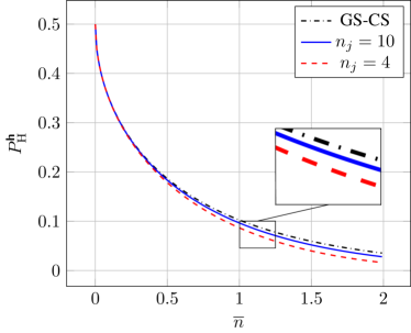
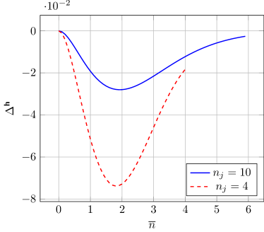
Figure 2. Helstrom bounds are plotted for GS-CS and spin CS with $n_{j}=4$ and $10$. The spin SC Helstrom bound is slightly lower, for any value $\bar{n}\leq n_{j}$. Left: Helstrom bound as function of $\bar{n}$. Right: Delta function, (6.18) versus $\bar{n}$.

6.2. SU$(1,1)$-CS as optical CS

The application in quantum optics of coherent states built from representations of the non-compact group SU$(1,1)$ lying in the discrete series has been carried out by various authors, see for instance the noticeable papers by Wodkiewicz and Eberly [Wodkiewicz-Eberly 1985], Gerry [Gerry 1987], Brif [Brif 1995]. See also in [Hach et al 2016, Hach et al 2018] (and references therein) the interesting properties revealed by such states when they are entangled.

6.2.1. Perelomov CS

This set of states derives from Perelomov SU$(1,1)$-CS [Perelomov 1972, Perelomov 1986], here again adapted to the context of quantum optics. They emerge through the unitary action of SU$(1,1)$ on number states. This leads to an infinite-dimensional Fock Hilbert space $\mathcal{H}$ with $\alpha$ constrained to the open disk, $\mathcal{D}:=\{\alpha\in\mathbb{C}\,,\,|\alpha|<1\}$. When the Fock state is the vacuum and $\varkappa>1/2$, the Perelomov $\varkappa$-dependent CS are the following NL-CS:

(6.11) $$|\alpha;\varkappa\rangle_{\mathrm{Per}}=\sum_{n=0}^{\infty}\alpha^{n}\,h_{n}\left(|\alpha|^{2}\right)\,|n\rangle\,,\quad h_{n}(u)=\lambda_{n}(1-u)^{\varkappa}\,,\quad\lambda_{n}=\sqrt{\binom{2\varkappa-1+n}{n}}\,,\quad x_{n}=\frac{n}{2\varkappa-1+n}\,.$$

The corresponding generalised exponential is the binomial (also called $q$-exponential in different contexts, see [Bergeron et al 2012] and references therein):

(6.12) $$\mathcal{N}(u)=(1-u)^{-2\varkappa}\,.$$

They solve the identity:

(6.13) $$\frac{2\varkappa-1}{\pi}\int_{\mathcal{D}}\frac{\mathrm{d}^{2}\alpha}{\left(1-|\alpha|^{2}\right)^{2}}\,|\alpha;\varkappa\rangle_{\mathrm{Per}}{}_{\mathrm{Per}}\langle\alpha;\varkappa|=\mathbb{1}\,.$$

This results in a negative binomial distribution, [Ali et al 2008],

(6.14) $$n\mapsto\mathsf{P}_{n}(u)=(1-u)^{2\varkappa}\,\binom{2\varkappa-1+n}{n}\,u^{n}\,.$$

While the number operator average value takes the form

(6.15) $$\bar{n}(u)=2\varkappa\,\frac{u}{1-u}\ \Leftrightarrow\ u={\frac{\bar{n}/2\varkappa}{1+\bar{n}/2\varkappa}}\,.$$

Note that introducing the efficiency $\eta:=\dfrac{1}{2\varkappa}\in(0,1)$ allows to express the probability (6.14) as a function of the scaled average photocount number $\bar{N}:=\eta\bar{n}$,

(6.16) $$\mathsf{P}_{n}(u)\equiv\widetilde{\mathsf{P}}_{n}(\bar{N})=(1+\bar{N})^{-1/\eta}\binom{1/\eta-1+n}{n}\,\left(\frac{\bar{N}}{1+\bar{N}}\right)^{n}\,.$$

This distribution has a notable property to reduce to Bose-Einstein distribution at the bound $\eta=1$, which corresponds to the limit $\varkappa=1/2$ of SU$(1,1)$ discrete series. At sub-unit efficiency, $\eta<1$, i.e. $\varkappa>1/2$, deviation from the Bose-Einstein distribution can be interpreted as resulting from using the scaled average value $\bar{N}$ (detected photons) in place of the mean value $\bar{n}$ of photons effectively reaching the detector (not all detected) [Fox 2006, Aharonov et al 2011].

Then, applying (5.14) with (6.12), i.e., $F(u)=-2\varkappa\ln(1-u)$, provides the Mandel parameter,

(6.17) $$Q_{M}(u)=\frac{u}{1-u}\ \Leftrightarrow\ \widetilde{Q}_{M}(\bar{n})=\frac{\bar{n}}{2\varkappa}\,.$$

It follows that contrarily to the previous case the states (6.11) are super-Poissonian. This result could be expected from the above discussion about their thermal nature. The functions $\bar{n}(u)$ and $\widetilde{Q_{M}}(\bar{n})$ are plotted in Figure 3 for $\varkappa=2$ and $5$.

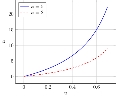
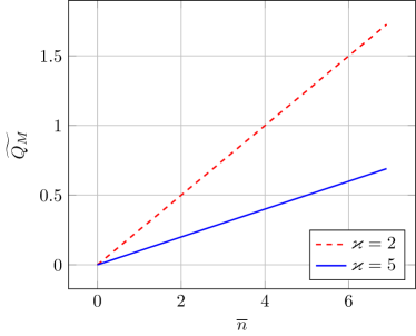
Figure 3. Photon statistics for Perelomov SU$(1,1)$-CS with $\varkappa=2$ and 5. These states are always super-Poissonian. Left: Average value of photons $\bar{n}$ as a function of the parameter $u$ (6.15). Right: Mandel parameter $\widetilde{Q_{M}}$ (6.17) as a function of $\bar{n}$.

Concerning the Helstrom bound, (4.5) becomes here

(6.18) $$\Delta(\bar{n})=\left(1+\frac{\bar{n}}{2\varkappa}\right)^{-2\varkappa}-e^{-\bar{n}}\,.$$

Applying the inequality (6.10) yields $\Delta(\bar{n})\geq 0$ for any $\bar{n}$ and $\kappa$. Note that $\Delta(\bar{n})\to 0$ as $\varkappa\to\infty$. Contrarily to the Perelomov spin $SU(2)$ CS above, the Helstrom bound is now larger than the GS-CS Helstrom bound for any value of $u=|\alpha|^{2}$, this is clearly shown in Figure 4. Here again, this result could be expected due to the “classical” thermal nature of the Perelomov SU$(1,1)$ coherent states.

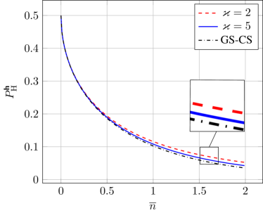
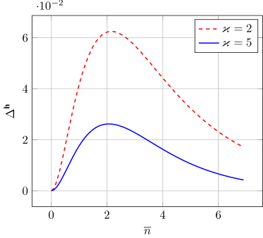
Figure 4. Helstrom bounds for GS-CS and Perelomov SU$(1,1)$-CS, with $\varkappa=2$ and 5, are compared. This latter states perform better than the former ones. Left: The Helstrom bound $P_{H}^{\boldsymbol{\mathsf{h}}}$ (4.3), for GS-CS and Perelomov SU$(1,1)$-CS. Right: The function $\Delta^{\boldsymbol{\mathsf{h}}}(\bar{n})$ (6.18).

6.2.2. Barut-Girardello CS

This set of nonlinear CS [Barut-Girardello 1971, Antoine et al 2001] belongs to the AN class. These are eigenstates of the lowering operator of SU$(1,1)$ in the discrete series representation $U^{\varkappa}$, with $\varkappa>1/2$. The related Fock space $\mathcal{H}$ is also infinite whereas $\alpha$ is allowed to assume any value in $\mathbb{C}$.

(6.19) $$|\alpha;\varkappa\rangle_{\mathrm{BG}}=\sum_{n=0}^{\infty}\alpha^{n}\,h_{n}\left(|\alpha|^{2}\right)\,|n\rangle\,,\quad h_{n}(u)=\frac{\lambda_{n}}{\sqrt{\mathcal{N}_{\mathrm{BG}}(u)}}\,,\quad\lambda_{n}=\sqrt{\frac{\Gamma(2\varkappa)}{n!\Gamma(2\varkappa+n)}}=\frac{1}{\sqrt{x_{n}!}}\,,$$

with $x_{n}=n(2\varkappa+n-1)$, and

(6.20) $$\mathcal{N}_{\mathrm{BG}}(u)=\Gamma(2\varkappa)\sum_{n=0}^{\infty}\frac{u^{n}}{n!\Gamma(2\varkappa+n)}=\Gamma(2\varkappa)\,u^{1/2-\varkappa}\,I_{2\varkappa-1}(2\sqrt{u})\,.$$

Here $I_{\nu}$ is a modified Bessel function of a first kind [Magnus et al 1966],

(6.21) $$I_{\nu}(z)=\left(\frac{z}{2}\right)^{\nu}\sum_{n=0}^{\infty}\frac{\left(\dfrac{z^{2}}{4}\right)^{n}}{n!\,\Gamma(\nu+n+1)}\,.$$

In this case the solution to the moment problem (5.6) reads as

(6.22) $$\int_{0}^{\infty}\mathrm{d}u\,w_{\mathrm{BG}}(u)\,\frac{u^{n}}{\mathcal{N}_{\mathrm{BG}}(u)}=x_{n}!\,,\quad w_{\mathrm{BG}}(u)=\mathcal{N}_{\mathrm{BG}}(u)\,\frac{2}{\Gamma(2\varkappa)}\,u^{\varkappa-1/2}\,K_{2\varkappa-1}(2\sqrt{u})\,,$$

with $K_{\nu}$ being the second modified Bessel function. This naturally leads to the resolution of the identity:

(6.23) $$\int_{\mathbb{C}}\frac{\mathrm{d}^{2}\alpha}{\pi}\,w_{\mathrm{BG}}\left(|\alpha|^{2}\right)\,|\alpha;\varkappa\rangle_{\mathrm{BG}}{}_{\mathrm{BG}}\langle\alpha;\varkappa|=\mathbb{1}\,.$$

The associated mean values (5.8) and (5.11), and the Mandel parameter have been calculated in [Antoine et al 2001], together with their asymptotic behavior at large $u$. They read respectively:

(6.24) $$\bar{n}(u)=\sqrt{u}\frac{I_{2\varkappa}(2\sqrt{u})}{I_{2\varkappa-1}(2\sqrt{u})}\underset{\mathrm{large}\,u}{\approx}\sqrt{u}-\varkappa+\frac{1}{4}+\mathrm{O}\left(\frac{1}{\sqrt{u}}\right)\quad\mbox{and}\quad\underset{\mathrm{small}\,u}{\approx}\frac{u}{2\varkappa}\left(1-\frac{u}{2\varkappa\,(1+2\varkappa)}\right)\,,$$

(6.25) $$\overline{n^{2}}(u)=\bar{n}(u)+u\frac{I_{2\varkappa+1}(2\sqrt{u})}{I_{2\varkappa-1}(2\sqrt{u})}\underset{\mathrm{large}\,u}{\approx}u+(1-2\varkappa)\sqrt{u}\quad\underset{\mathrm{small}\,u}{\approx}\frac{u}{2\varkappa}\left(1-\frac{(1-2\varkappa)\,u}{2\varkappa\,(1+2\varkappa)}\right)\,,$$

(6.26) $$Q_{M}(u)=\sqrt{u}\left[\frac{I_{2\varkappa+1}(2\sqrt{u})}{I_{2\varkappa}(2\sqrt{u})}-\frac{I_{2\varkappa}(2\sqrt{u})}{I_{2\varkappa-1}(2\sqrt{u})}\right]\underset{\mathrm{large}\,u}{\approx}-\frac{1}{2}+\frac{1}{16}(-3+16\varkappa-16\varkappa^{2})\sqrt{\frac{1}{u}}\quad\mbox{and}\quad\underset{\mathrm{small}\,u}{\approx}-\frac{u}{2\varkappa\,(1+2\varkappa)}\,.$$

Thus, the asymptotic behavior at large $u$ of the mean square error reads $(\Delta n)^{2}\approx\sqrt{u}/2$. Moreover, it follows from the inequality $\left(I_{\nu+1}(x)\right)^{2}\geq I_{\nu}(x)\,I_{\nu+2}(x)$ for all $x\geq 0$ that contrarily to the previous Perelomov SU$(1,1)$ case, the states (6.19) are sub-Poissonian. The function $\bar{n}(u)$ and the Mandel parameter for the Barut-Girardello SU$(1,1)$ CS, with parameters $\varkappa=1/2,2,5$, are shown in Figure 5.

As to the Helstrom bound, (4.5) becomes here

(6.27) $$\Delta(\bar{n})=\left[\Gamma(2\varkappa)\,(u(\bar{n}))^{1/2-\varkappa}\,I_{2\varkappa-1}\left(2\sqrt{u(\bar{n})}\right)\right]^{-1}-e^{-\bar{n}}=\frac{\widetilde{\Delta}(\bar{n})}{e^{\bar{n}}\,\Gamma(2\varkappa)\,(u(\bar{n}))^{1/2-\varkappa}\,I_{2\varkappa-1}\left(2\sqrt{u(\bar{n})}\right)}\,,$$

where

(6.28) $$\widetilde{\Delta}(\bar{n}):=e^{\bar{n}}-\Gamma(2\varkappa)\,(u(\bar{n}))^{1/2-\varkappa}\,I_{2\varkappa-1}(2\sqrt{u(\bar{n})})\,.$$

Helstrom bounds ($P_{H}^{\boldsymbol{\mathsf{h}}}(\bar{n})$ and $\Delta^{\boldsymbol{\mathsf{h}}}(\bar{n})$) for GS-CS and Barut-Girardello SU$(1,1)$ CS are compared in Figure 6. Like for the spin CS, we notice that the Helstrom bound is lower than the GS-CS Helstrom bound for any value of $u=|\alpha|^{2}$.

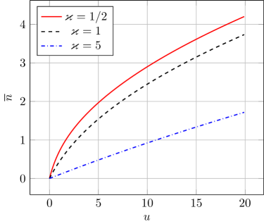
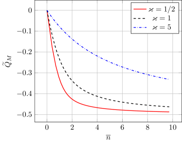
Figure 5. Photon statistics for Barut-Girardello SU$(1,1)$ CS with $\varkappa=1/2,2$ and $5$. Left: Average value of photons $\bar{n}$ as a function of the parameter $u$. Right figure: The Mandel parameter $\widetilde{Q_{M}}$ as a function of $\bar{n}$ is always negative, which makes the present states sub-Poissonian.

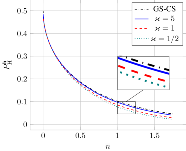
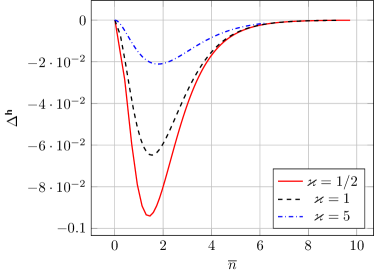
Figure 6. Left: The Helstrom bounds for GS-CS and Barut-Girardello SU$(1,1)$ CS, with $\varkappa=1/2,2$ and $5$, are compared. Right: Delta function (6.28). We notice that the difference of the Helstrom bounds increases as $\varkappa$ decreases.

7. NL-CS from deformed binomial distributions

We now turn our attention to an important subclass of the non-linear coherent states (5.5) associated with a sequence $\boldsymbol{\chi}$ of positive numbers $x_{n}$ for $n>0$ and $x_{0}=0$. Their construction is based on the deformation of the binomial distribution which was used in the Bernouilli transform (2.16) in order to take into account the imperfection of the detection encoded by the parameter $\eta$. The rationale behind such deformations was to keep the property (2.17) enjoyed by the GS-CS’s, for which imperfect detection amounts to replace $\alpha$ by $\sqrt{\eta}\alpha$ (2.18), while the deformed binomial expression is a well defined probability distribution. This means that we examine this replacement as an alternative to the change $\bar{n}\mapsto\eta\bar{n}$ in (4.10) – note that the latter is not equivalent to (2.18). This aim was at the origin of the series of works [Curado et al 2010], [Curado et al 2012], [Bergeron et al 2012], [Bergeron et al 2013], where two of us were involved. We distinguish between asymmetric and symmetric deformations of the binomial distribution.

7.1. Asymmetric deformations

From the sequence $\boldsymbol{\chi}=(x_{0},x_{1},\dotsc,x_{n},\dotsc)$, $x_{0}=0$ and $x_{n}>0$ for $n>0$, we build the formal normalised distribution

(7.1) $$\mathfrak{p}_{k}^{(n)}(\eta)=\frac{x_{n}!}{x_{n-k}!\,x_{k}!}\,\eta^{k}\,p_{n-k}(\eta)\,,\quad\sum_{k=0}^{n}\mathfrak{p}_{k}^{(n)}(\eta)=1\,.$$

The polynomials $p_{s}(\eta)$ satisfy $p_{s}(0)=1$, $p_{s}(1)=0$, for all $s$, and the sequence $(p_{s})_{n\in\mathbb{N}}$ is determined by recurrence: $p_{0}(\eta)=1\,,\ p_{1}(\eta)=1-\eta,\dotsc$ If $p_{m}(\eta)\geq 0$ for all $m$ and $\eta\in[0,1]$, then a probabilistic interpretation is valid, and $\eta=\langle x_{k}\rangle_{n}/x_{n}$. A noticeable outcome is that

(7.2) $$G_{\mathcal{N},\eta}(u):=\frac{\mathcal{N}(u)}{\mathcal{N}(\eta u)}=\sum_{s=0}^{\infty}p_{s}(\eta)\frac{u^{s}}{x_{s}!}\,,\quad\mathcal{N}(u)=\sum_{n}\frac{u^{n}}{x_{n}!}\,,$$

is the generating function of the polynomials $p_{s}(\eta)$. This is important in order to find explicitly all sequences $\boldsymbol{\chi}$ for which the Bernouilli-like distribution (7.1) obeys the positiveness condition, i.e., it is a genuine probability distribution. As a consequence, using an alphabet based on the NL-CS (5.5), the probability $\mathsf{P}_{n}(u;\eta)$ to detect $n$-photons with sub-unit efficiency, $\eta<1$, is given in terms of the perfect, $\eta=1$, detector probability (5.7), $\mathsf{P}_{m}(u;\eta=1)=u^{m}/(\mathcal{N}(u)x_{m}!)$, $u=|\alpha|^{2}$, by the deformed Bernoulli transform:

(7.3) $$\mathsf{P}_{n}(u;\eta)=\sum_{m=n}^{\infty}\frac{x_{m}!}{x_{m-n}!\,x_{n}!}\,\eta^{n}\,p_{m-n}(\eta)\,\mathsf{P}_{m}(u;\eta=1)=\frac{(\eta\,u)^{n}}{\mathcal{N}(\eta u)\,x_{n}!}\,.$$

This discrete probability distribution corresponds to the normalized states $|\sqrt{\eta}\alpha;\boldsymbol{\chi}\rangle$, being equivalent to the family of non-linear coherent states defined by (5.5) through the rescaling (2.18).

One can interpret such deformation as a modification of the probability of getting $k$ wins (photon clicks) in a total of $n$ events. With $y_{0}=0$, $y_{n}=x_{n}/n$ for $n>0$ $\mathfrak{p}_{k}^{(n)}(\eta)$ gives the probability to get $k$ wins and $n-k$ losses, while

(7.4) $$\pi_{k}^{(n)}(\eta)\stackrel{{\scriptstyle\mathrm{def}}}{{=}}\frac{\mathfrak{p}_{k}^{(n)}(\eta)}{\binom{n}{k}}=\dfrac{y_{n}!}{y_{n-k}!\,y_{k}!}\,\eta^{k}\,p_{n-k}(\eta)$$

stands for the probability of one given string having $k$ wins and $n-k$ losses. Such a deformation means there are correlations between different events. We call this distribution asymmetric because $\mathfrak{p}_{k}^{(n)}(\eta)$ is not invariant under $k\to n-k$ and $\eta\to 1-\eta$, as it would hold for the binomial case. Due to this asymmetry, there might be bias in favor of either win or loss, including when $\eta=1/2$.

A comprehensive analysis exploring generating functions to examine the positiveness condition $p_{m}(\eta)\geq 0$ for all $m$ and $\eta\in[0,1]$ and finding the solutions was exposed in [Bergeron et al 2012]. It starts with $\mathcal{N}(u)$ which gives the generating function of $p_{k}(\eta)$ through the relation (7.2). Let $\Sigma$ be the set of entire series $\mathcal{N}(u)=\sum_{n=0}^{\infty}a_{n}u^{n}$ having a strictly positive radius of convergence and verifying the conditions $a_{0}=1$ and $\forall n\geq 1,\,a_{n}>0$. Let us associate with $\mathcal{N}$ the sequence $x_{n}=a_{n-1}/a_{n}=n\,\mathcal{N}^{(n-1)}(0)/\mathcal{N}^{(n)}(0)$ so that $a_{n}=1/(x_{n}!)$. Next let $\Sigma_{0}$ be the set of entire series $\sum_{n=0}^{\infty}a_{n}z^{n}$ having a strictly positive radius and verifying $a_{0}=0$, $a_{1}>0$ and $\forall n\geq 2,\,a_{n}\geq 0$. It was proved in [Bergeron et al 2012] that $\Sigma_{+}:=\left\{\mathcal{N}\in\Sigma\,|\,\forall\eta\in[0,1),\,p_{n}(\eta)>0\,\right\}=\{e^{F}\,|\,F\in\Sigma_{0}\}$ is the set of deformed exponentials with generating functions $G_{\mathcal{N},\eta}(u)$ that do solve the positiveness problem. All sequences $\boldsymbol{\chi}$ with this probabilistic content are called sequences of complete statistical type, or CST.

One can add to this probabilistic interpretation of the above defined asymmetric deformed binomial distribution the Poisson-like limit behaviour. Indeed, if the sequence $\{x_{n}\}_{n\in\mathbb{N}}$ is such that, , at fixed $m$, $\underset{n\to\infty}{\lim}{\frac{x_{n-m}}{x_{n}}}=1$, then the limit when $n\to\infty$ of $\mathfrak{p}_{k}^{(n)}(\eta)$, given by (7.1), with $\eta=u/x_{n}$ is equal to $\frac{1}{\mathcal{N}(u)}\,\frac{u^{k}}{x_{k}!}$.

This allows to better comprehend the behaviour of CST sequences in comparison with natural integers. In fact, when picking a $\mathcal{N}\in\Sigma_{+}$; its related CST sequence $x_{n}=n\,\mathcal{N}^{(n-1)}(0)/\mathcal{N}^{(n)}(0)$ verifies $0\leq x_{n}\leq nx_{1}.$ We give now two examples (see [Bergeron et al 2012] for more).

7.1.1. Example 1

Let $\{a_{n}\}_{n\in\mathbb{N}}$ be a sequence of positive real numbers with $\sum_{n=0}^{\infty}a_{n}<\infty$. Given $\zeta\in[0,1]$ the function $\mathcal{N}(u)=\prod_{k=0}^{\infty}(1+\zeta a_{k}u)/(1-a_{k}u)$ belongs to $\Sigma_{+}$, see [Bergeron et al 2012]. One gets a simple illustration with $\mathcal{N}(u)=(1-au)^{-m}=\sum_{k=0}^{\infty}(u^{k})/(x_{k}^{(m)}!)\,,$ where $a>0$. The convergence radius is $1/a$, and the the resulting sequence is equivalent, up to a variable rescaling, to the Perelemov SU$(1,1)$ case (6.12), $x_{k}^{(m)}!=k!\,(m-1)!/a^{k}(m-1+k)!,$ and $x_{k}^{(m)}=k/(a(m-1+k).$ It is worth noting that at the limit $k\rightarrow\infty$ all coefficients $x_{k}^{(m)}$ go to the limit $x_{\infty}^{(m)}=1/a$. Moreover, the resulting polynomial probabilities $p_{k}(\eta)$, $0\leq\eta\leq 1$, are hypergeometrical $p_{k}(m;\eta)={}_{2}F_{1}(-m,-k;1-k-m;\eta).$ For example, with $n=2$, the probability of having two wins in a set of two trials is similar to the binomial case, yet the probability to get one win and one loss is smaller and the probability to get two losses is higher in comparison to the binomial one. Nonetheless the sum of all three possibilities is equal to one, as required.

7.1.2. Example 2

Another example is yielded by the function

(7.5) $$\mathcal{N}(u)=\exp\left(u+\frac{a}{2}u^{2}\right)\,\quad a>0\,.$$

The convergence radius is infinite, as for the exponential function. The associated generating function reads $G_{\mathcal{N},\eta}(u)=\exp\left((1-\eta)t+\frac{a}{2}(1-\eta^{2})u^{2}\right)\,.$ The corresponding $x_{n}!$ are expressed in terms of Hermite polynomials:

(7.6) $$x_{n}!=\left[\frac{\mathsf{i}^{n}\left(\frac{a}{2}\right)^{n/2}}{n!}H_{n}\left(\frac{-\mathsf{i}}{\sqrt{2a}}\right)\right]^{-1}=\left[\sum_{m=0}^{\left\lfloor\frac{n}{2}\right\rfloor}\frac{(a/2)^{m}}{m!(n-2m)!}\right]^{-1}\,.$$

and we have the asymptotic behavior $x_{n}\sim\sqrt{n/a}+\cdots\,.$
The average average value of number of photons is given by

(7.7) $$\bar{n}(u)=u(1+au)\quad\Leftrightarrow\quad u(\bar{n})=\frac{1}{2a}\left(\sqrt{1+4a\bar{n}}-1\right)\,.$$

The Mandel parameter is

(7.8) $$Q_{M}(u)=\frac{au}{1+au}\quad\Leftrightarrow\quad\widetilde{Q_{M}}(\bar{n})=\frac{\sqrt{1+4a\bar{n}}-1}{\sqrt{1+4a\bar{n}}+1}\,,$$

and is positive for all possible values of $\bar{n}$, as shown in the Fig. 7. The related states are thus all super-Poissonian, as is the case for all NL-CS based on deformed binomial distributions, see Sec. 7.3.

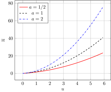
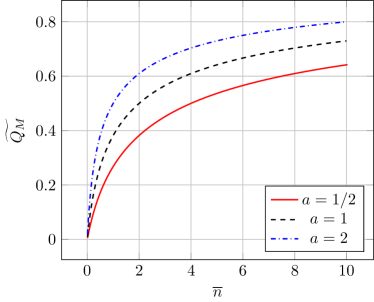
Figure 7. Photon statistics for Hermite polynomials CS with $a=1/2,1$ and $2$. Left: $\bar{n}$ as function of $u$. Right: Mandel parameter versus $\bar{n}$. We notice that it is positive, which makes these states super-Poissonian, as is the case for all NL-CS based on deformed binomial distributions, see Sec. 7.3.

The function $\Delta^{\boldsymbol{\mathsf{h}}}(\bar{n})$ given by (4.6) reads

(7.9) $$\Delta(\bar{n})=e^{\frac{1}{4a}-\frac{\bar{n}}{2}-\frac{1}{4a}\sqrt{1+4a\bar{n}}}-e^{-\bar{n}}\,,$$

and is always positive, that is the Helstrom bound is higher than for GS-CS, see Fig. 8.

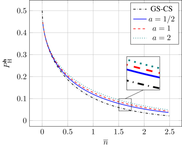
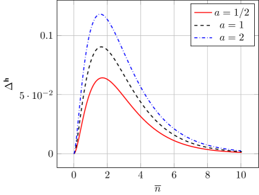
Figure 8. Helstrom bounds for GS-CS and Hermite polynomials CS, with $a=1/2,1$ and $2$, are compared. Left: Helstrom bounds as function of $\bar{n}$ for several values of $a$. The Helstrom bound is higher than GS-CS, which means that the quantum error limit is larger than for GS-CS states, as is the case for all NL-CS based on deformed binomial distributions, see Sec. 7.3. Right: Delta function (7.9) versus $\bar{n}$.

7.2. Symmetric deformations

The following symmetric option was explored in [Bergeron et al 2013]:

(7.10) $$\mathfrak{p}_{k}^{(n)}(\eta)=\dfrac{x_{n}!}{x_{n-k}!x_{k}!}q_{k}(\eta)q_{n-k}(1-\eta)\\ ,$$

with $q_{k}(\eta)$ being polynomials of degree $k$. Normalization and non-negativeness conditions constrain the $\mathfrak{p}_{k}^{(n)}(\eta)$ through

(7.11) $$\begin{split}&\sum_{k=0}^{n}\mathfrak{p}_{k}^{(n)}(\eta)=1\quad\forall n\in\mathbb{N},\quad\forall\eta\in[0,1]\,,\\ &\mathfrak{p}_{k}^{(n)}(\eta)\geq 0\quad\forall n,k\in\mathbb{N},\quad\forall\eta\in[0,1]\,.\end{split}$$

The normalization implies $\mathfrak{p}_{0}^{(0)}(\eta)=q_{0}(\eta)q_{0}(1-\eta)=1\Rightarrow q_{0}(\eta)=\pm 1$, $\forall\eta\in[0,1]$. Assuming $q_{0}(\eta)=1$ we have $\mathfrak{p}_{0}^{(n)}(\eta)=q_{n}(1-\eta).$ Also the positiveness condition corresponds to the positiveness of the polynomials $q_{n}$, for $\eta\in[0,1]$. Like for the asymmetric case, the polynomials $\mathfrak{p}_{k}^{(n)}(\eta)$ might be interpreted as the probability to get $k$ wins and $n-k$ failures in a string of $n$ trials. In both cases there is correlation between different trials. However, since the invariance under $k\to n-k$ and $\eta\to 1-\eta$ holds as for the binomial distribution, no bias can exist favoring either win or failure for $\eta=1/2$.

An appealing example of generating functions gives rise to binomial-type polynomials. Let us pick a $x_{n}$-generating function $\mathcal{N}(u)\in\Sigma$. Then we have

(7.12) $$\forall\eta\in[0,1],\quad\tilde{G}_{\mathcal{N},\eta}(u):=\mathcal{N}(u)^{\eta}=\sum_{n=0}^{\infty}\dfrac{q_{n}(\eta)}{x_{n}!}u^{n}.$$

Because $q_{0}(\eta)=1$ and $\forall n\neq 0,q_{n}(0)=0$, the positiveness condition implies that the function $\mathcal{N}(u)^{\eta}$ belongs to $\Sigma$. Furthermore, It was proven in [Bergeron et al 2013] that if $\mathcal{N}(u)\in\Sigma_{+}$, then the polynomials $\mathfrak{p}_{k}^{(n)}(\eta)$ allow a probabilitic interpretation. Moreover one finds that the expectation value of the $k$ variable takes the simple form $\langle k\rangle_{n}=\eta n\,,$ as in the usual binomial case.

A first illustration of symmetric deformations is found from the Perelomov SU$(1,1)$ type (6.12) (up to a rescaling of the variable) with $\mathcal{N}(u)=\left(1-u/s\right)^{-s}\,,\quad s>0\,.$ This gives the sequence $x_{n}=ns/(n+s-1)$ with $\lim_{n\to\infty}x_{n}=s.$ The corresponding polynomials are $q_{n}(\eta)=(s\eta)_{n}/(s)_{n},$ where $(x)_{n}=\Gamma(x+n)/\Gamma(x)$ (Pochhammer symbol). In addition to the mean value expression $\langle k\rangle_{n}=\eta n$, the square root of the variance $(\sigma_{k})_{n}=n\sqrt{\eta(1-\eta)}\sqrt{(1+s/n)/(1+s)}$ also becomes proportional to the mean value at large $n$.

7.2.1. Example: The modified Abel polynomials

(7.13) $$\mathcal{N}(t)=e^{-\beta W(-u/\beta)}\,,\quad\beta>0\,,$$

with $W$ being the Lambert function. The latter is defined implicitly through $W(u)e^{W(u)}=u$. It is worth noting that if $\beta\to\infty$ thus $\mathcal{N}(u)\to e^{u}$. This leads to a sequence which is bounded by $\beta/e$:

(7.14) $$x_{n}=\frac{n\beta}{n+\beta}\left(1-\frac{1}{n+\beta}\right)^{n-2}\,,\quad\lim_{n\to\infty}x_{n}=\beta/e\,.$$

One can also notice that $x_{n}\to n$ as $\beta\to\infty$. This results into the following factorials:

(7.15) $$x_{n}!=n!\,\frac{\beta^{n-1}}{(n+\beta)^{n-1}}\,.$$

The polynomials $q_{n}$’s read

(7.16) $$q_{n}(\eta)=\eta\frac{\left(\eta+\frac{n}{\beta}\right)^{n-1}}{\left(1+\frac{n}{\beta}\right)^{n-1}}\,.$$

Note that $q_{0}(\eta)=1$ and $q_{1}(\eta)=\eta$. The probability distribution (7.10) reads in this case

(7.17) $$\mathfrak{p}_{k}^{(n)}(\eta)=\binom{n}{k}\eta(1-\eta)\frac{(\eta+k/\beta)^{k-1}(1-\eta+(n-k)/\beta)^{n-k-1}}{(1+n/\beta)^{n-1}}\,.$$

The average value of photons and Mandel parameter are then given by

(7.18) $$\bar{n}(u)=-\frac{\beta W\left(-\frac{u}{\beta}\right)}{1+W\left(-\frac{u}{\beta}\right)}\,,\qquad Q_{M}(u)=\frac{1}{\left(1+W\left(-\frac{u}{\beta}\right)\right)^{2}}-1\,.$$

The inversion $u(\bar{n})$ is done here numerically in order to get the Mandel parameter and Helstrom bound as a function of $\bar{n}$. These states are super-Poissonian (see Fig. 9), and lead to a Helstrom bound higher than the GS-CS case (see Fig. 10).

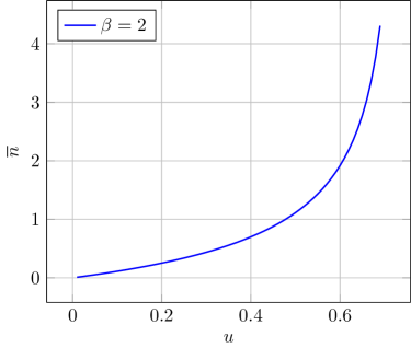
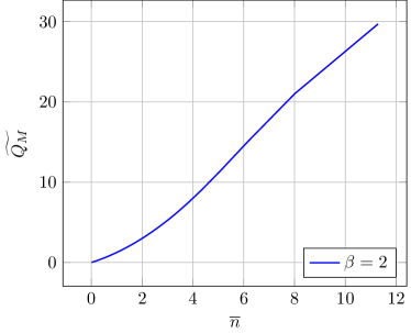
Figure 9. Photon statistics for modified Abel polynomials CS with $\beta=2$. Left: $\bar{n}$ as function of $u$. Right: Mandel parameter versus $\bar{n}$. We notice that it is positive, which makes these states super-Poissonian, as is the case for all NL-CS based on deformed binomial distributions, see Sec. 7.3.

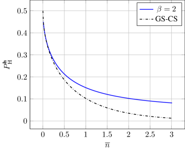
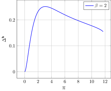
Figure 10. Helstrom bounds for GS-CS and modified Abel polynomials CS with $\beta=2$ are compared. Left: Helstrom bounds as function of $\bar{n}$. Right: Delta function (7.9) versus $\bar{n}$. The Delta function is always positive as is the case for all NL-CS based on deformed binomial distributions, see Sec. 7.3.

7.3. Quasi-classical nature of CS associated with asymmetric and symmetric binomial deformations

We now show that the above results, namely states are super-Poissonian and HB is higher compared to GS-CS, hold for any symmetric or asymmetric deformation of the binomial law. Let us consider a generic deformed exponential defined through

(7.19) $$\mathcal{N}(u)=\sum_{n=0}^{\infty}\frac{u^{n}}{x_{n}!},$$

and demonstrate that this always yields positive Mandel parameter and $\Delta(\bar{n})$.

Proposition 7.1.

Symmetric and asymmetric binomial deformations defined through (7.1) and (7.10), respectively, lead to super-Poissonian NL-CS.

Proof.

This can easily be shown by considering the sequence $\{x_{n}\}$ generated by $\mathcal{N}(u)\in\Sigma_{+}$. Expressing $\mathcal{N}$ as $\mathcal{N}(u)=e^{F(u)}\in\Sigma_{+}$, with $F(u)=\sum_{k=1}^{\infty}a_{k}u^{k}$, we have

(7.20) $$\overline{n^{2}}-\overline{n}^{2}-\overline{n}=\sum_{k=1}^{\infty}(k^{2}-k)a_{k}u^{k}\,.$$

Since $\forall n\geq 2$ $a_{n}\geq 0$, the right-hand side of (7.20) is positive. Consequently the Mandel parameter $Q_{M}$, defined through (3.15), is positive. $\square$

Proposition 7.2.

If $\mathcal{N}(u)\in\Sigma_{+}$, the NL-CS cannot optimize the Helstrom bound

Proof.

In [Bergeron et al 2012] one can establish the proof from the following statements:

• For all $\mathcal{N}\in\Sigma_{+}$, $\ln\mathcal{N}\in\Sigma_{0}$ and

  (7.21) $$\ln\mathcal{N}(u)=\sum_{k=1}^{\infty}\frac{(-p^{\prime}_{k}(1))}{x_{k}!}\frac{u^{k}}{k}\,,$$

• $p^{\prime}_{1}(1)=-1$ and $p^{\prime}_{n}(1)\leq 0$  .

Using (7.21) we get

(7.22) $$u\frac{d}{du}\ln\mathcal{N}(u)=\sum_{k=1}^{\infty}\frac{(-p^{\prime}_{k}(1))}{x_{k}!}u^{k}\,.$$

Since $u>0$, we conclude that

(7.23) $$\ln\mathcal{N}(u)<u\frac{\mathrm{d}}{\mathrm{d}u}\ln\mathcal{N}(u)\,,$$

which can be written as

(7.24) $$\frac{1}{\mathcal{N}(u)}>e^{-u\frac{\mathrm{d}}{\mathrm{d}u}\ln\mathcal{N}(u)}\,.$$

The expression above, once expressed in terms of $\bar{n}$, leads to

(7.25) $$\left|h_{0}(u(\overline{n}))\right|^{2}>e^{-\overline{n}}\,.$$

Therefore, the $\Delta_{h}$ function is always positive and therefore the Helstrom bound is larger than in the GS-CS case. $\square$

8. Mandel parameter and Helstrom bound for both Susskind-Glogower and modified Susskind-Glogower CS

Here we examine the Susskind-Glogower CS’s [Susskind-Glogower 1964] which exhibit attractive properties on different levels, as shown in [Montel-Moya-Cessa 2011, Montel et al 2011, Moya-Cessa and Soto-Eguibar 2011]. On the mathematical side, they are built through the action of the unitary displacement operator on the Fock vacuum state, see for instance [Récamier et al 2008].

(8.1) $$\mathbb{R}\ni x\mapsto|x\rangle_{\mathrm{SG}}=D_{\mathrm{SG}}(x)|0\rangle\equiv e^{x(V^{{\dagger}}-V)}|0\rangle\,.$$

The operator $V$ and its adjoint $V^{{\dagger}}$ are the shift operators in the Fock space:

(8.2) $$V=\sum_{n=0}^{\infty}|n\rangle\langle n+1|\,,\quad V^{{\dagger}}=\sum_{n=0}^{\infty}|n+1\rangle\langle n|\,,\quad[V,V^{{\dagger}}]=\mathbb{1}-|0\rangle\langle 0|\,.$$

The normalised states (8.1) expand in terms of number states as:

(8.3) $$|x\rangle_{\mathrm{SG}}=\sum_{n=0}^{\infty}(n+1)\,\frac{J_{n+1}(2x)}{x}\,|n\rangle\,,$$

where $J_{\nu}$ is the Bessel function,

(8.4) $$J_{\nu}(z)=\left(\frac{z}{2}\right)^{\nu}\,\sum_{m=0}^{\infty}\frac{(-1)^{m}\left(\frac{z}{2}\right)^{2m}}{m!\,\Gamma(\nu+m+1)}\,.$$

Normalisation implies the interesting identity whose proof is given in the appendix of [Montel et al 2011]:

(8.5) $$\sum_{n=1}^{\infty}n^{2}\,\left(J_{n}(2x)\right)^{2}=x^{2}\,.$$

On the physical side, the authors of [Montel et al 2011] showed that the coherent states (8.3) may be modeled by propagating light in semi-infinite arrays of optical fibers.

Now, the expression (8.4) can be used to extend (8.3) in a non analytic way to a complex $\alpha$ as

(8.6) $$(n+1)\frac{J_{n+1}(2x)}{x}\mapsto\alpha^{n}\,(n+1)\sum_{m=0}^{\infty}\frac{(-1)^{m}|\alpha|^{2m}}{m!\,\Gamma(n+m+2)}\equiv\alpha^{n}\,h^{\mathrm{SG}}_{n}(|\alpha|^{2})\,,$$

i.e.,

(8.7) $$h^{\mathrm{SG}}_{n}(u)=(n+1)\,\frac{1}{u^{\frac{n+1}{2}}}\,J_{n+1}(2\sqrt{u})\,,$$

and thus

(8.8) $$|\alpha\rangle_{\mathrm{SG}}=\sum_{n=0}^{\infty}\alpha^{n}\,h^{\mathrm{SG}}_{n}(|\alpha|^{2})\,|n\rangle\,.$$

The moment equation (3.5) reads here

(8.9) $$\int_{0}^{\infty}\mathrm{d}u\,\frac{w(u)}{u}\,\left(J_{n}(2\sqrt{u})\right)^{2}=2\int_{0}^{\infty}\mathrm{d}t\,\frac{w(t^{2})}{t}\,\left(J_{n}(2t)\right)^{2}=\frac{1}{n^{2}}\,,$$

and appear not to have an immediate solution. On the other hand, by examining the following integral formula for Bessel functions [Magnus et al 1966],

(8.10) $$\int_{0}^{\infty}\frac{\mathrm{d}t}{t}\,\left(J_{n}(2t)\right)^{2}=\frac{1}{2n}\,.$$

we are led to replace the SG-CS of (8.3) by the modified Susskind-Glogower coherent states (SGm-CS):

(8.11) $$|\alpha\rangle_{\mathrm{SGm}}=\sum_{n=0}^{\infty}\alpha^{n}\,h^{\mathrm{SGm}}_{n}(|\alpha|^{2})\,|n\rangle\,,\quad h^{\mathrm{SGm}}_{n}(u)=\sqrt{\frac{n+1}{\mathcal{N}(u)}}\,\frac{1}{u^{\frac{n+1}{2}}}\,J_{n+1}(2\sqrt{u})\,,$$

with

(8.12) $$\mathcal{N}(u)=\frac{1}{u}\sum_{n=1}^{\infty}n\,\left(J_{n}(2\sqrt{u})\right)^{2}=\frac{1}{u}\left[2u\left(J_{0}(2\sqrt{u})\right)^{2}-\sqrt{u}J_{0}(2\sqrt{u})J_{1}(2\sqrt{u})+2u\left(J_{1}(2\sqrt{u})\right)^{2}\right]\,.$$

The formula (8.10) then can be used to demonstrate that the resolution of the identity (3.9) is satisfied for SGm-CS $|\alpha\rangle_{\mathrm{SGm}}$ with $w(u)=\mathcal{N}(u)$.

(8.13) $$\int_{\mathbb{C}}\frac{\mathrm{d}^{2}\alpha}{\pi}\,\mathcal{N}\left(|\alpha|^{2}\right)\,|\alpha\rangle_{\mathrm{SGm}}{}_{\mathrm{SGm}}\langle\alpha|=\mathbb{1}\,.$$

Mean values (5.8) and (5.11) read respectively:

(8.14) $$\bar{n}(u)=\frac{1}{\mathcal{N}(u)}-1\,,$$

(8.15) $$\overline{n^{2}}(u)=-\frac{2}{\mathcal{N}(u)}+\frac{4}{3}(2u+1)-\frac{u\left(J_{0}(2\sqrt{u})\right)^{2}-u\left(J_{1}(2\sqrt{u})\right)^{2}+\sqrt{u}J_{0}(2\sqrt{u})J_{1}(2\sqrt{u})}{3u\mathcal{N}(u)}\,.$$

For comparison, Mandel parameters for SG-CS and SGm-CS are plotted in Figure 11. It results that the SG-CS and SGm-CS are sub-Poissonian for $\bar{n}\lesssim 22$ and $\bar{n}\lesssim 10$) respectively.

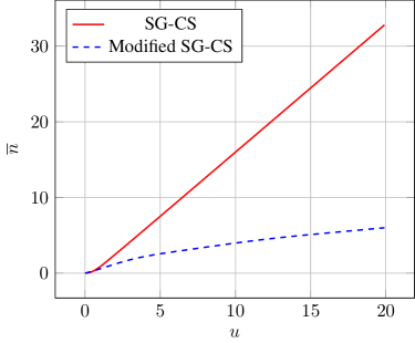
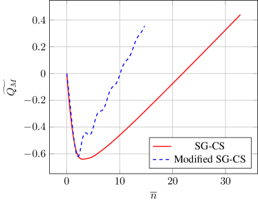
Figure 11. Photon statistics for SG-CS and modified SGm-CS. Left: $\bar{n}$ as function of $u$. Right: Mandel parameter versus $\bar{n}$. We notice that the SG-CS and SGm-CS are sub-Poissonian for $\bar{n}\lesssim 22$ and $\bar{n}\lesssim 10$ respectively.

As to the Helstrom bound, (4.5) becomes

(8.16) $$\Delta(\bar{n}(u))=\frac{\left(J_{1}(2\sqrt{u})\right)^{2}}{u\mathcal{N}(u)}-e^{1-1/\mathcal{N}(u)}\,.$$

This is compared to both SG and GS coherent states in Figure 12. Astonishingly the Helstrom bounds vanishes for some specific values of $\bar{n}$ in the two cases of GS-CS and GSm-CS. Taking the logarithm makes it easier to see for which values of $\bar{n}$ the Helstrom bounds reaches zero, this happens for $\bar{n}$ around two in both cases.

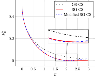
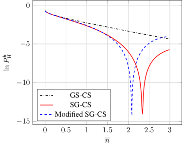
Figure 12. Helstrom bounds for GS-CS, SG-CS and modified SG-CS are compared. Left figure: Helstrom bound $P_{H}^{\boldsymbol{\mathsf{h}}}$ (4.3), for GS-CS, SG-CS and modified SGm-CS. Right figure: Natural logarithm of the Helstrom bound $\ln P_{H}^{\boldsymbol{\mathsf{h}}}$, for GS-CS, SG-CS and SGm-CS, which makes it easier to see for which values of $\bar{n}$ the Helstrom bounds reaches zero.

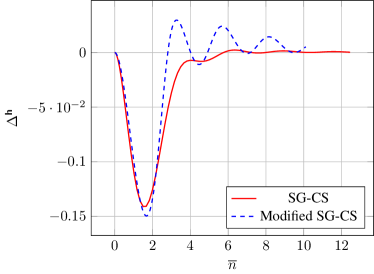
Figure 13. Function $\Delta^{\boldsymbol{\mathsf{h}}}(\bar{n})$ for SG-CS and modified SG-CS. The Helstrom bounds for GS-CS and GSm-CS oscillate as $\bar{n}$ is varying and, actually, do also vanish for higher values of $\bar{n}$. Yet the difference with GS-CS gets lower and so does $\Delta^{\boldsymbol{\mathsf{h}}}(\bar{n})$.

9. Conclusion

In this work we have examined statistical properties of various generalizations of the Glauber-Sudarshan coherent states within the framework of Quantum Optics, namely Fock spaces of one-mode photons. In particular we analysed the Mandel parameter and more importantly the quantum error limit, or Helstrom bound. We have proved the classical or quasi-classical nature of a whole family of non-linear coherent states, those based on symmetric and asymmetric deformations of the binomial distribution, in the sense that they are super-Poissonian and do not improve the GS-CS Helstrom bound.

We have also revealed the deep quantum nature of four other families of NL-CS, namely the Perelomov Spin CS’s, the SU$(1,1)$ Barut-Girardello CS’s, the Susskind-Glogower CS’s, and their modified version: they are sub-Poissonian and improve more or less significantly the GS-CS Helstrom bound. In particular, the SG-CS’s and SGm-CS’s turn out to exhibit an astonishing result: the Helstrom bound vanishes for some values of the average photons number $\bar{n}$, the smallest being around $\bar{n}=2$. This means that these states are then orthogonal to the vacuum state. Consequently it appears possible to use coherent states for binary communication with no quantum error, nevertheless, limited to specific values of $\bar{n}$.

In a parent work we will focus our attention on the modified Susskind-Glogower CS. These, unlike the SG-CS, obeys the normalisation (3.5), which in turn implies the resolution of the identity in the Fock space (3.9), or (8.13) in the present case. Finally, we will explore their physical feasibility and relevance in the spirit of [Montel et al 2011].

References

- [Holevo 1973] A. S. Holevo, Statistical decision theory for quantum systems, J. Multivariate Anal. 3 (1973) 337394.
- [Holevo 2011] A. S. Holevo, Probabilistic and statistical aspects of quantum theory, Quaderni/Monographs, 1. Edizioni della Normale, Pisa, 2011.
- [Fuchs 1996] C. A. Fuchs, Distinguishability and Accessible Information in Quantum Theory, Ph.D. thesis, University of New Mexico, 1996.
- [Peres 1995] A. Peres, Quantum Theory: Concepts and Methods. Kluwer Academic Publishers, Dordrecht, 1995.
- [Bennet&Brassard 1984] C. H. Bennett and G. Brassard, in Proceedings of the IEEE International Conference on Computers, Systems abd Signal Processing IEEE, New York, 1984, 175.
- [Helstrom 1976] C. W. Helstrom. Quantum Detection and Estimation Theory. Academic Press, New York, 1976.
- [Cook et al 2007] R. L. Cook, P. J. Martin, and J. M. Geremia, Optical coherent state discriminationusing a closed-loop quantum measurement, Nature, 446 (2007) 774.
- [Tsujino et al 2011] K. Tsujino, D. Fukuda, G. Fujii, S. Inoue, M. Fujiwara, M. Takeoka, and M. Sasaki, Quantum receiver beyond the standard quantum limit of coherent optical communication, Phys. Rev. Lett., 106 (2011) 250503.
- [Becerra et al 2013] F. E. Becerra, J. Fan, G. Baumgartner, J. Goldhar, J. T. Kosloski and A. Migdall, Experimental demonstration of a receiver beating the standard quantum limit for multiple nonorthogonal state discrimination, Nat. Photonics, 7(2) (2013) 147.
- [Kunz et al 2019] L. Kunz et al., Beating the Standard Quantum Limit for Binary Constellations in the Presence of Phase Noise, 21st International Conference on Transparent Optical Networks (ICTON) (2019).
- [Sych & Leuchs 2016] D. Sych and G. Leuchs, Practical Receiver for Optimal Discrimination of Binary Coherent Signals, Phys. Rev. Lett. 117 (2016) 200501.
- [DiMario et al 2019] M. T. DiMario, et al., Optimized Communication Strategies with Binary Coherent States over Phase Noise Channels, npj Quantum Information 5 (2019) 65.
- [Gazeau 2009] J.-P. Gazeau, Coherent States in Quantum Physics. Wiley-VCH, Berlin, 2009.
- [Perina 1984] J. Periña Quantum Statistics of Linear and Nonlinear Optical Phenomena. Reidel, Dordrecht, 1984.
- [Perina 1994] J. Periña (Editor). Coherence and Statistics of Photons and Atoms. Wiley-Interscience, 2001.
- [Tse et al 2019] M. Tse et al. Quantum-Enhanced Advanced LIGO Detectors in the Era of Gravitational-Wave Astronomy, Phys. Rev. Lett. 123 (2019) 231107.
- [Acernese et al 2019] F. Acernese et al., Increasing the Astrophysical Reach of the Advanced Virgo Detector via the Application of Squeezed Vacuum States of Light, Phys. Rev. Lett. 123 (2019) 231108.
- [Gazeau 2019] J.-P. Gazeau, Coherent states in Quantum Optics: An oriented overview, Integrability, Supersymmetry and Coherent States, A volume in honour of V. Hussin, Eds. Kuru, Sengul, Negro, Javier, Nieto, Luis M., CRM series in Mathematical Physics. Springer, (2019) 69-101;
- [Curado et al 2010] E. M. F. Curado, J.-P. Gazeau, and L. M .C. S. Rodrigues, Non-linear coherent states for optimizing Quantum Information, Proceedings of the Workshop on Quantum Nonstationary Systems, October 2009, Brasilia. Comment section (CAMOP) Phys. Scr., 82 (2010) 038108.
- [Curado et al 2012] E. M. F. Curado, J.-P. Gazeau, and Ligia M. C. S. Rodrigues, On a Generalization of the Binomial Distribution and Its Poisson-like Limit, J. Stat. Phys., 146 (2012) 264-280.
- [Bergeron et al 2012] H. Bergeron, E. M. F. Curado, J.-P. Gazeau, and Ligia M. C. S. Rodrigues, Generating functions for generalized binomial distributions, J. Math. Phys., 53 (2012) 103304-1-22.
- [Bergeron et al 2013] H. Bergeron, E. M. F. Curado, J.-P. Gazeau, and Ligia M. C. S. Rodrigues, Symmetric generalized binomial distributions, J. Math. Phys., 54 (2013) 123301-1-22.
- [Moya-Cessa and Soto-Eguibar 2011] H. M. Moya-Cessa and F. Soto-Eguibar, Introduction to Quantum Optics. Rinton Press, Paramus, 2011.
- [Loudon 1973] R. Loudon. The Quantum Theory of Light. Oxford Univ. Press, Oxford, 1973.
- [Geremia 2004] J. M. Geremia, Distinguishing between optical coherent states with imperfect detection, Phys. Rev. A 70 (2004) 062303-1-9.
- [Akhiezer 1965] N. I. Akhiezer, The classical moment problem and some related questions in analysis, translated from the Russian by N. Kemmer, Hafner Publishing Co., New York, 1965.
- [Perelomov 1972] A. M. Perelomov, Coherent States for Arbitrary Lie Group, Commun. math. Phys., 26 (1972) 222-236.
- [Perelomov 1986] A. M. Perelomov, Generalized Coherent States and Their Applications. Springer, Berlin (1986).
- [Fox 2006] M. Fox, Quantum Optics: An Introduction. Oxford University Press, New York (2006).
- [Ali et al 2008] S. T. Ali, J.-P. Gazeau, and B. Heller, Coherent states and Bayesian duality, J. Phys. A: Math. Theor., 41 (2008) 365302-1-22.
- [Wodkiewicz-Eberly 1985] K. Wodkiewicz and J. Eberly, Coherent states, squeezed fluctuations, and the SU and SU groups in quantum-optics applications. J. Opt. Soc. B, 2 (1985) 458.
- [Gerry 1987] C. C. Gerry, Application of SU coherent states to the interaction of squeezed light in an anharmonic oscillator, Phys. Rev. A, 35 (1987) 2146.
- [Brif 1995] C. Brif, Photon states associated with the Holstein-Primakoff realization of the SU Lie algebra Quantum Semiclass. Opt., 7 (1995) 803.
- [Hach et al 2016] E. E. Hach III, P. M. Alsing, and C. C. Gerry, Violations of a Bell in- equality for entangled SU coherent states based on dichotomic observables, Phys. Rev. A, 93 (2016) 042104.
- [Hach et al 2018] E. E. Hach III, R. BirritellaI, P. M. Alsing, and C. C. Gerry, SU parity and strong violations of a Bell inequality by entangled Barut-Girardello coherent states, J. Opt. Soc. B, 35 (2018) 2433.
- [Aharonov et al 2011] Y. Aharonov, E. C. Lerner, H. W. Huang, and J. M. Knight, Oscillator phase states, thermal equilibrium and group representations, J. Math. Phys., 14 (2011) 746-755.
- [Barut-Girardello 1971] A. O. Barut and L. Girardello, New “Coherent” States Associated with Non-Compact Groups, Commun. Math. Phys., 21 (1971) 41-55.
- [Antoine et al 2001] J.-P. Antoine, J.-P. Gazeau, J. R. Klauder, P. Monceau, and K. A. Penson, J. Math. Phys., 42 (2001) 2349-2387.
- [Magnus et al 1966] W. Magnus, F. Oberhettinger, and R. P. Soni. Formulas and Theorems for the Special Functions of Mathematical Physics. Springer-Verlag, Berlin, Heidelberg and New York (1966).
- [Susskind-Glogower 1964] L. Susskind and J. Glogower, Quantum mechanical phase and time operator, Phys. Phys. Fiz. 1, 1 (1964) 49-61.
- [Montel-Moya-Cessa 2011] R. De J. León Montel and H. M. Moya-Cessa, Modeling non-linear coherent states in fiber arrays, Int. J. Quant. Information, 9 (2011) Suppl. 349-355.
- [Montel et al 2011] R. De J. León Montel, H. M. Moya-Cessa and F. Soto-Eguibar, Nonlinear coherent states for the Susskind-Glogower operators, Rev. Mex. Fís., 57 (2011) 133-147.
- [Récamier et al 2008] J. Récamier, M. Gorayeb, W. L. Mochán, and J. L. Paz, Nonlinear Coherent States and Some of Their Properties, Int. J. Theor. Phys., 47 (2008) 673-683.