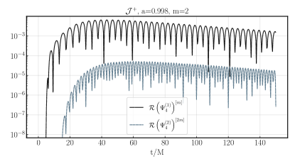
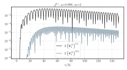
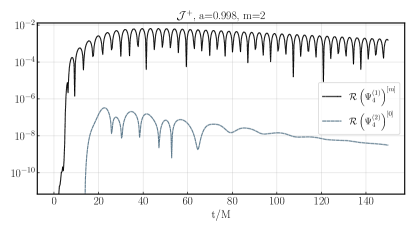
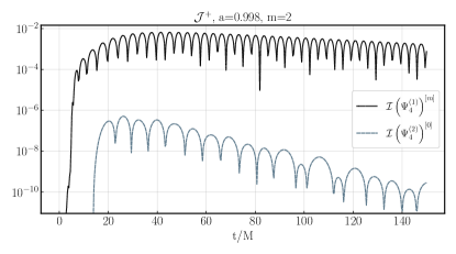
Numerical computation of second order vacuum perturbations of Kerr black holes

Justin L. Ripley lloydripley@gmail.com DAMTP, Centre for Mathematical Sciences, University of Cambridge, Wilberforce Road, Cambridge CB3 0WA, UK.    Nicholas Loutrel nloutrel@princeton.edu Department of Physics, Princeton University, Princeton, New Jersey 08544, USA.    Elena Giorgi egiorgi@princeton.edu Department of Mathematics, Princeton University, Princeton, New Jersey 08544, USA. Princeton Gravity Initiative, Princeton University, Princeton, New Jersey 08544, USA.    Frans Pretorius fpretori@princeton.edu Department of Physics, Princeton University, Princeton, New Jersey 08544, USA. Princeton Gravity Initiative, Princeton University, Princeton, New Jersey 08544, USA.
Abstract

Motivated by the desire to understand the leading order nonlinear gravitational wave interactions around arbitrarily rapidly rotating Kerr black holes, we describe a numerical code designed to compute second order vacuum perturbations on such spacetimes. A general discussion of the formalism we use is presented in Loutrel et al. (2020); here we show how we numerically implement that formalism with a particular choice of coordinates and tetrad conditions, and give example results for black holes with dimensionless spin parameters a=0.7𝑎0.7a=0.7 and a=0.998𝑎0.998a=0.998. We first solve the Teukolsky equation for the linearly perturbed Weyl scalar Ψ4(1)superscriptsubscriptΨ41\Psi_{4}^{(1)}, followed by direct reconstruction of the spacetime metric from Ψ4(1)superscriptsubscriptΨ41\Psi_{4}^{(1)}, and then solve for the dynamics of the second order perturbed Weyl scalar Ψ4(2)superscriptsubscriptΨ42\Psi_{4}^{(2)}. This code is a first step toward a more general purpose second order code, and we outline how our basic approach could be further developed to address current questions of interest, including extending the analysis of ringdown in black hole mergers to before the linear regime, exploring gravitational wave “turbulence” around near-extremal Kerr black holes, and studying the physics of extreme mass ratio inspiral.

I Introduction

In this paper we initiate a numerical study of the dynamics of second order vacuum perturbations of a Kerr black hole. Linear black hole perturbation theory has played an important role in the study of black holes, with diverse applications from mathematical physics to gravitational wave astrophysics (for reviews see e.g. Sasaki and Tagoshi (2003); Dafermos and Rodnianski (2013); Barack and Pound (2019)). Regarding the latter, it is used in interpreting the ringdown phase of a binary black hole merger, and for extreme mass ratio inspirals (EMRIs). For both of these physical regimes, it is presently computationally intractable to full numerical solution without recourse to perturbative methods.

For some applications it may be necessary to go beyond linear perturbations. Here for brevity we only mention a couple of key incentives (a more thorough discussion that motivates this study can be found in our companion paper Loutrel et al. (2020)). In order to extract subleading modes of the ringdown following comparable mass mergers, it may be necessary to consider nonlinear effects. The “problem” with such mergers is that the leading order quadrupole mode is excited with such high amplitude relative to subleading modes (see e.g. London et al. (2014, 2016)), that nonlinear mode coupling could produce features of similar strength to subleading modes; this is particularly so within the first few cycles of ringdown were most of the observable signal, hence most opportunity for measurement, lies. It will be important to quantitatively understand second order features to reap the most out of ringdown analysis of future loud merger events.

Nonlinear physics may also play an important role in the ringdown of near-extremal Kerr black holes111We note though that comparable mass mergers cannot produce near-extremal remnants, see e.g. Hemberger et al. (2013); Lousto and Zlochower (2014); Healy et al. (2014); Hofmann et al. (2016), and it is unknown how rapidly the typical supermassive black holes in the universe, of relevance to EMRIs, rotate. Thus near-extremal ringdown may end up being more a question of theoretical, rather than astrophysical, interest. . This can partly be motivated by the presence of a family of slowly damped modes, whose damping timescale grows without bound as the black hole spin approaches its extremal value  Detweiler (1980); Hod (2008); Yang et al. (2013)222Though there is some controversy about exactly what the spectrum of modes of extremal/near-extremal black holes is; see e.g. Hod (2015); Zimmerman et al. (2015); Hod (2016); Richartz (2016); Casals and Longo Micchi (2019).. The slower damping of perturbations implies nonlinear effects could be more pronounced; most intriguing in this regard is the suggestion that mode coupling induces a turbulent energy cascade in near-extremal Kerr black holes Yang et al. (2015), similar to that seen in a few studies of black holes and black branes in asymptotically Anti de-Sitter spacetime Carrasco et al. (2012); Green et al. (2014); Adams et al. (2014). Nonlinear effects almost certainly play some role in the physics of extremal Kerr black holes, as those have been shown to be linearly unstable Detweiler (1980); Aretakis (2015, 2013) (the instability may be related to the above mentioned slowly damped quasinormal modes, that become “zero damped” in the extremal limit).

Finally, we mention that second order black hole perturbation theory plays an important role in computing the second order self force of a small particle orbiting a black hole, which is relevant to modeling EMRIs (e.g. Barack (2009)). We note though that in this paper we only consider the second order vacuum perturbation of a Kerr black hole, so our results are not directly applicable to modeling EMRI physics.

Following a brief summary of our formalism in Sec.II.1 (which is described in more detail in our companion paper Loutrel et al. (2020)), in the remainder of this paper we describe a numerical implementation of the method and then analyze a few example runs from our code. In the remainder of the introduction we give a general overview of our numerical approach.

Several steps are required to arrive at the desired second order perturbation. First is to solve for a linear gravitational wave perturbation characterized by the Weyl scalar Ψ4subscriptΨ4\Psi_{4} (or equivalently Ψ0subscriptΨ0\Psi_{0}) using the Teukolsky equation Teukolsky (1973). As described in Sec. II.2, with more details given in Appendix C, we begin with the Kerr metric in Boyer-Lindquist form and a rotated version of the Kinnersley tetrad Kinnersley (1969), then transform these to a hyperboloidal compactified, horizon penetrating coordinate system. In these coordinates then we numerically solve the Teukolsky equation in the time domain, starting with Cauchy data for Ψ4(1)superscriptsubscriptΨ41\Psi_{4}^{(1)}. (We note that many codes have been developed over the years to solve the Teukolsky equation; see, e.g. Krivan et al. (1997, 1997); Baker et al. (2002); Lopez-Aleman et al. (2003); Lousto (2005); Burko and Khanna (2007); Sundararajan et al. (2007); Zenginoglu and Khanna (2011); Harms et al. (2013)).

Campanelli and Lousto first showed that the evolution of the second order perturbation of Ψ4subscriptΨ4\Psi_{4} is also governed by the Teukolsky equation, with a source term that depends on all components of the first order metric perturbation hμνsubscript𝜇𝜈h_{\mu\nu} Campanelli and Lousto (1999). The next step in our calculation the is therefore to reconstruct this first order metric correction from the first order perturbation of Ψ4subscriptΨ4\Psi_{4}. We directly reconstruct the metric by solving a set of nested null transport equations in the outgoing radiation gauge Chrzanowski (1975). Once this is complete, we numerically solve the Teukolsky equation in the time domain with the second order source term for the second order correction to Ψ4subscriptΨ4\Psi_{4}. This latter quantity is in general not invariant under first order gauge or tetrad transformations (see  Campanelli and Lousto (1999)); as discussed in Sec. III, in our coordinate system we can avoid these issues if we measure the waves at future null infinity in an asymptotically flat gauge, which is one reason why we employ a hyperboloidal slicing and the outgoing radiation gauge.
Refer to caption
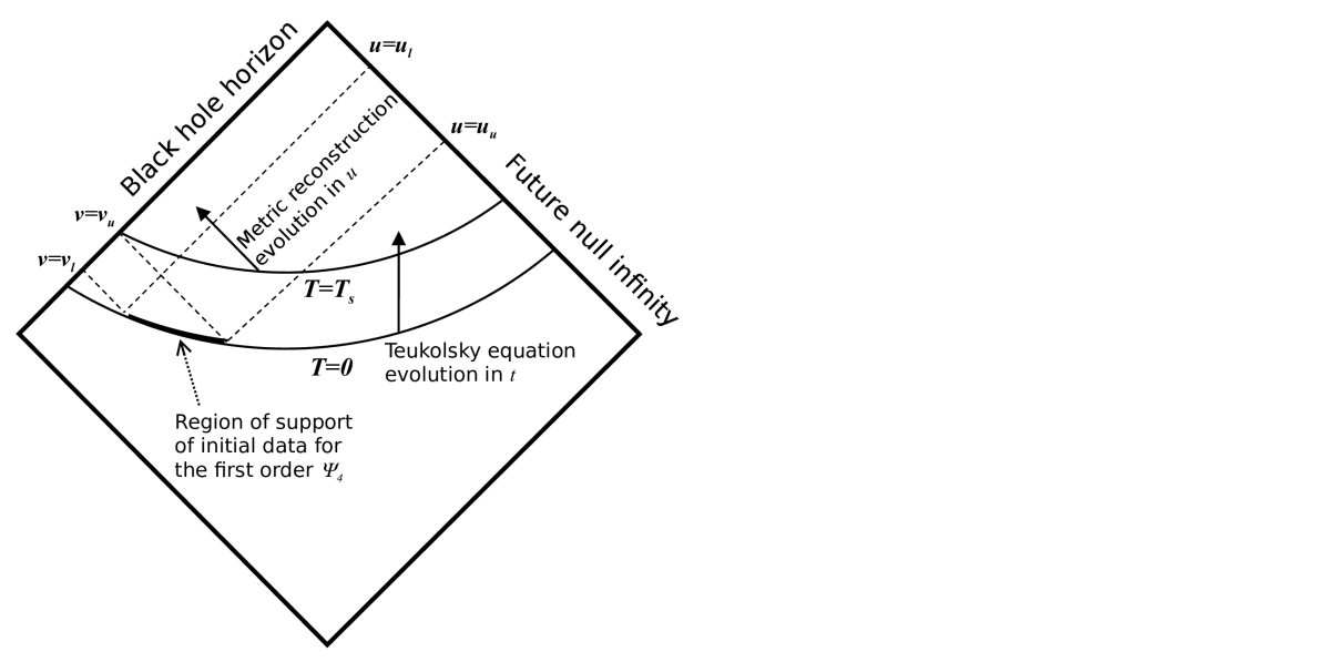
Figure 1: Schematic Penrose diagram demonstrating the domains of evolution and metric reconstruction. The Teukolsky equation is integrated using a Cauchy evolution scheme along hypersurfaces of constant time T𝑇T, whereas metric reconstruction is carried out using null transport equations in the u𝑢u direction, with characteristics tangent to the ingoing Newman-Penrose vector nμsuperscript𝑛𝜇n^{\mu}. We provide initial data for the first order Ψ4(1)superscriptsubscriptΨ41\Psi_{4}^{(1)} at T=0𝑇0T=0, with compact support in radial distance from the black hole in the range r=(rl,ru)𝑟subscript𝑟𝑙subscript𝑟𝑢r=(r_{l},r_{u}), intersecting a range in advanced (retarded) time of u=(uu,ul)𝑢subscript𝑢𝑢subscript𝑢𝑙u=(u_{u},u_{l}) (v=(vl,vu)𝑣subscript𝑣𝑙subscript𝑣𝑢v=(v_{l},v_{u})). Thus only in the region u>uu,T>0,formulae-sequence𝑢subscript𝑢𝑢𝑇0u>u_{u},T>0, does the spacetime differ from Kerr, which allows for trivial initial data for the first order metric reconstruction equations along u=uu𝑢subscript𝑢𝑢u=u_{u}. For simplicity, as explained in the text, we begin evolution of the second order perturbation Ψ4(2)superscriptsubscriptΨ42\Psi_{4}^{(2)} at T=Ts𝑇subscript𝑇𝑠T=T_{s}; in a sense then this is our “true” initial data surface for the gravitational wave perturbation of Kerr calculated to second order. For technical reasons explained in Sec. IV, this initial data setup only leads to consistent metric reconstruction if Ψ4(1)superscriptsubscriptΨ41\Psi_{4}^{(1)} has azimuthal mode content |m|2𝑚2|m|\geq 2.

One difficulty with using null transport equations in conjunction with the (3+1) Cauchy evolution scheme we use for the Teukolsky equation is that their domains of integration do not “easily” overlap. An implication of this is if we wanted to solve for the second order perturbation over the entire domain of our Cauchy evolution we would need to solve a set of first order constraint equations on the initial T=0𝑇0T=0 slice to give self-consistent initial data for the reconstruction equations. As explained more in Sec. IV and illustrated in Fig. 1, we avoid this issue here by choosing initial data for the first-order Ψ4(1)superscriptsubscriptΨ41\Psi_{4}^{(1)} that has compact support on the initial slice, and only solve for the first order metric beginning on an ingoing null slice (vusubscript𝑣𝑢v_{u}) intersecting T=0𝑇0T=0 outside of this region (as we explain in Fig. 1, our metric reconstruction equations are transport equations along the ingoing null tetrad vector nμsuperscript𝑛𝜇n^{\mu}). Then, initial data for reconstruction only needs to be specified along the outgoing null curves u=uu𝑢subscript𝑢𝑢u=u_{u}, which is trivially the Kerr solution. In principle we could immediately begin the second order evolution for vvu𝑣subscript𝑣𝑢v\geq v_{u}, though again to simplify the Cauchy evolution we only start second order evolution at a constant hyperboloidal time Tssubscript𝑇𝑠T_{s} after all the ingoing data from vlsubscript𝑣𝑙v_{l} to vusubscript𝑣𝑢v_{u} has entered the black hole horizon. The Cauchy evolution prior to this is then, in a sense, simply providing a map from initial data for the first order Ψ4(1)superscriptsubscriptΨ41\Psi_{4}^{(1)} specified on T=0𝑇0T=0 to the “true” initial time T=Ts𝑇subscript𝑇𝑠T=T_{s}. As implemented in the code, during each step of the Cauchy evolution we also perform reconstruction (and second order integration for T>Ts𝑇subscript𝑇𝑠T>T_{s}). The reconstruction will therefore not be consistent until evolution crosses v=vu𝑣subscript𝑣𝑢v=v_{u}, but for illustrative purposes we also show independent residuals of our reconstruction procedure prior to that, to demonstrate that the inconsistency then has no effect on the consistency of the solution afterward.

As described in Sec.V, we use pseudo-spectral methods to solve both the Teukolsky and null transport equations; the code can be downloaded from Ripley (2020a). Example results are given in Sec. VI.1 and Sec. VI.2 for a black hole with dimensionless spin a=0.7𝑎0.7a=0.7 and a=0.998𝑎0.998a=0.998 respectively. Specifically, for the examples we consider the linear wave only contains azimuthal eimϕsuperscript𝑒𝑖𝑚italic-ϕe^{im\phi} angular dependence for m=2𝑚2m=2. This linear field sources a second order Ψ4(2)superscriptsubscriptΨ42\Psi_{4}^{(2)} containing modes with both m=0𝑚0m=0 and m=4𝑚4m=4. We conclude in Sec. VII, which includes a discussion of how our methods and code will be extended to tackle the problems we are ultimately interested in addressing.

In Appendix A we describe the conventions we use for the Fourier transform and normalization of discrete quantities used to display some of our results. In Appendix B we provide a derivation of the metric reconstruction equations and second order source term in the specific gauge and coordinates used here, which is slightly different from the analytical example case give in Loutrel et al. (2020). We describe the transformation of the Kerr metric and Kinnersley tetrad in Boyer-Lindquist coordinates to the coordinates we use in the code in Appendix C. Finally, in Appendix D we collect some useful properties of spin-weighted spherical harmonics, which are used in our pseudo-spectral code.

I.1 Notation and conventions

We use geometric units (8πG=18𝜋𝐺18\pi G=1, c=1𝑐1c=1) and follow the definitions and sign conventions of Chandrasekhar Chandrasekhar (2002) (in particular the ++--- signature for the metric), except we use Greek letters μ,ν𝜇𝜈\mu,\nu... to denote spacetime indices. We use the non-standard symbols : ϖ=3.14159italic-ϖ3.14159\varpi=3.14159... for the number ‘pi’ (to avoid confusion with the Newman-Penrose scalar π𝜋\pi), and the symbols \mathcal{R} and \mathcal{I} to respectively denote the real and imaginary parts of fields. We use an overbar f¯¯𝑓\bar{f} to denote complex conjugation of a quantity f𝑓f.

We write the perturbed metric gμνsubscript𝑔𝜇𝜈g_{\mu\nu} about a background solution gμν(0)superscriptsubscript𝑔𝜇𝜈0g_{\mu\nu}^{(0)} as gμν=gμν(0)+hμνsubscript𝑔𝜇𝜈superscriptsubscript𝑔𝜇𝜈0subscript𝜇𝜈g_{\mu\nu}=g_{\mu\nu}^{(0)}+h_{\mu\nu}, where hμνsubscript𝜇𝜈h_{\mu\nu} is the first order perturbation. Other than the metric, we denote an nthsuperscript𝑛𝑡n^{th} order quantity in a perturbative expansion with a trailing superscript (n)𝑛\ {}^{(n)}; e.g. the Newman-Penrose scalar Ψ2=Ψ2(0)+Ψ2(1)subscriptΨ2superscriptsubscriptΨ20superscriptsubscriptΨ21\Psi_{2}=\Psi_{2}^{(0)}+\Psi_{2}^{(1)} to linear order. However, for brevity, in terms of expressions where the correction to a background quantity will lead to a higher order perturbation than considered, we drop the (0) superscript from the background quantity. For example, in the Teukolsky equation, Eq. (II.1) below, all symbols other than Ψ4(1)superscriptsubscriptΨ41\Psi_{4}^{(1)} are background quantities.

II Description of the Scheme

In this section we summarize details of the reconstruction scheme and second order perturbation equation described in  Loutrel et al. (2020) that are particular to our numerical implementation.

II.1 Use of the NP/GHP formalisms

We make extensive use of the Newman-Penrose (NP)Newman and Penrose (1962) formalism. In the Appendix of the companion paper Loutrel et al. (2020) we gave a brief overview of the NP formalism, and to avoid excessive repetition we do not reproduce that here. However, we now mention the most salient definitions of the NP formalism necessary to understand the main points of this paper.

The NP formalism decomposes the geometry and Einstein equations in terms of an orthonormal basis of null vectors, {lμ,nμ,mμ,m¯μ}superscript𝑙𝜇superscript𝑛𝜇superscript𝑚𝜇superscript¯𝑚𝜇\{l^{\mu},n^{\mu},m^{\mu},\bar{m}^{\mu}\}; lμsuperscript𝑙𝜇l^{\mu} (nμsuperscript𝑛𝜇n^{\mu}) is an outgoing (ingoing) real null vector, and mμsuperscript𝑚𝜇m^{\mu} is a complex angular null vector with m¯μsuperscript¯𝑚𝜇\bar{m}^{\mu} its complex conjugate. These define the four directional derivative operators

D𝐷\displaystyle{D} =\displaystyle= lμμ,Δ=nμμ,superscript𝑙𝜇subscript𝜇Δsuperscript𝑛𝜇subscript𝜇\displaystyle l^{\mu}\partial_{\mu}\,,\qquad{\Delta}=n^{\mu}\partial_{\mu}\,, (1)
δ𝛿\displaystyle{\delta} =\displaystyle= mμμ,δ¯=m¯μμ.superscript𝑚𝜇subscript𝜇¯𝛿superscript¯𝑚𝜇subscript𝜇\displaystyle m^{\mu}\partial_{\mu}\,,\qquad\bar{{\delta}}=\bar{m}^{\mu}\partial_{\mu}\,. (2)

A vacuum geometry is characterized by the 5 complex scalars {Ψ0,Ψ1,Ψ2,Ψ3,Ψ4}subscriptΨ0subscriptΨ1subscriptΨ2subscriptΨ3subscriptΨ4\{\Psi_{0},\Psi_{1},\Psi_{2},\Psi_{3},\Psi_{4}\}, which are contractions of the Weyl tensor with various products of the null tetrad. The complex spin coefficients (essentially combinations of Ricci rotation coefficients, the tetrad analogue of the connection in a metric formalism) are {α,β,γ,ϵ,ρ,λ,π,μ,ν,τ,σ,κ}𝛼𝛽𝛾italic-ϵ𝜌𝜆𝜋𝜇𝜈𝜏𝜎𝜅\{\alpha,\beta,\gamma,\epsilon,\rho,\lambda,\pi,\mu,\nu,\tau,\sigma,\kappa\}. We choose a null tetrad, the explicit form of which is given later, such that for the background Kerr solution Ψ0=Ψ1=Ψ3=Ψ4=σ=κ=ν=λ=0subscriptΨ0subscriptΨ1subscriptΨ3subscriptΨ4𝜎𝜅𝜈𝜆0\Psi_{0}=\Psi_{1}=\Psi_{3}=\Psi_{4}=\sigma=\kappa=\nu=\lambda=0 (which is always possible for a general type D background) and γ=0𝛾0\gamma=0 (which is always possible when the background is Kerr).

In the NP formalism, perturbations of the Kerr spacetime lead to one master equation for the linearly perturbed Weyl scalar Ψ4subscriptΨ4\Psi_{4} known as the Teukolsky equation Teukolsky (1973), specifically

𝒯Ψ4(1)[(Δ+4μ+μ¯)(D+4ϵρ)\displaystyle\mathcal{T}\Psi_{4}^{(1)}\equiv\big{[}\left(\Delta+4\mu+\bar{\mu}\right)\left(D+4\epsilon-\rho\right)
(ð+4πτ¯)(ðτ)3Ψ2]Ψ4(1)=0.\displaystyle-\left(\textnormal{\dh}^{\prime}+4\pi-\bar{\tau}\right)\left(\textnormal{\dh}-\tau\right)-3\Psi_{2}\big{]}\Psi_{4}^{(1)}=0. (3)

(Here we have made use of the GHP operators ð and ðsuperscriptð\textnormal{\dh}^{\prime}, which we define in Eq. (4).) The first step of our procedure is to solve the Teukolsky equation for Ψ4(1)superscriptsubscriptΨ41\Psi_{4}^{(1)}. We discuss how we numerically solve this equation in Sec. V.1.

We also make some use of the Geroch-Held-Penrose (GHP) Geroch et al. (1973) formalism; in particular we use the following GHP derivatives acting on some NP scalar η𝜂\eta

ðη(δpβqα¯)η,ð𝜂𝛿𝑝𝛽𝑞¯𝛼𝜂\displaystyle\textnormal{\dh}\eta\equiv\left(\delta-p\beta-q\bar{\alpha}\right)\eta, (4a)
ðη(δ¯pαqβ¯)η,superscriptð𝜂¯𝛿𝑝𝛼𝑞¯𝛽𝜂\displaystyle\textnormal{\dh}^{\prime}\eta\equiv\left(\bar{\delta}-p\alpha-q\bar{\beta}\right)\eta, (4b)

where {p,q}𝑝𝑞\{p,q\} are the (constant) weights of η𝜂\eta (related to its spin and boost weights).

II.2 Choice of background coordinates and tetrad

We choose a form for the background Kerr metric, with mass and spin parameters M𝑀M and a𝑎a respectively, that is horizon penetrating and hyperboloidally compactified so that the constant time T𝑇T (spacelike) slices become asymptotically null, reaching future null infinite at finite coordinate radius. An outline of how we derive these coordinates is given in Appendix C; here we simply summarize their most important qualities.

We use a rotated version of the Kinnersley tetrad that is regular at future null infinity; in (T,R,ϑ,ϕ)𝑇𝑅italic-ϑitalic-ϕ(T,R,\vartheta,\phi) component form, the tetrad vectors read:

lμ=superscript𝑙𝜇absent\displaystyle l^{\mu}= R2L4+a2R2cos2ϑ(2M(2M(aL)2R),\displaystyle\frac{R^{2}}{L^{4}+a^{2}R^{2}\mathrm{cos}^{2}\vartheta}\bigg{(}2M\left(2M-\left(\frac{a}{L}\right)^{2}R\right),
12(L22MR+(aL)2R2),0,a),\displaystyle-\frac{1}{2}\left(L^{2}-2MR+\left(\frac{a}{L}\right)^{2}R^{2}\right),0,a\bigg{)}, (5a)
nμ=superscript𝑛𝜇absent\displaystyle n^{\mu}= (2+4MRL2,R2L2,0,0),24𝑀𝑅superscript𝐿2superscript𝑅2superscript𝐿200\displaystyle\left(2+\frac{4MR}{L^{2}},\frac{R^{2}}{L^{2}},0,0\right), (5b)
mμ=superscript𝑚𝜇absent\displaystyle m^{\mu}= R2(L2iaRcosϑ)(iasinϑ,0,1,isinϑ).𝑅2superscript𝐿2𝑖𝑎𝑅cositalic-ϑ𝑖𝑎sinitalic-ϑ01𝑖sinitalic-ϑ\displaystyle\frac{R}{\sqrt{2}\left(L^{2}-iaR\mathrm{cos}\vartheta\right)}\left(-ia\mathrm{sin}\vartheta,0,-1,-\frac{i}{\mathrm{sin}\vartheta}\right). (5c)

Here R𝑅R is the compactified radial coordinate, related to the Boyer-Lindquist radial coordinate by

rL2R,𝑟superscript𝐿2𝑅\displaystyle r\equiv\frac{L^{2}}{R}, (6)

with L𝐿L a constant parameter (R=0𝑅0R=0 thus corresponds to future null infinity).

With this tetrad and metric, the only nonzero Weyl scalar is

Ψ2=MR3(L2iaRcos(ϑ))3,subscriptΨ2𝑀superscript𝑅3superscriptsuperscript𝐿2𝑖𝑎𝑅cositalic-ϑ3\displaystyle\Psi_{2}=-\frac{MR^{3}}{\left(L^{2}-iaR\mathrm{cos}\left(\vartheta\right)\right)^{3}}, (7)

and the nonzero spin coefficients are

ρ=𝜌absent\displaystyle\rho= R(a2R2+L42L2MR)2(L2iaRcos(ϑ))2(L2+iaRcos(ϑ)),𝑅superscript𝑎2superscript𝑅2superscript𝐿42superscript𝐿2𝑀𝑅2superscriptsuperscript𝐿2𝑖𝑎𝑅italic-ϑ2superscript𝐿2𝑖𝑎𝑅italic-ϑ\displaystyle-\frac{R\left(a^{2}R^{2}+L^{4}-2L^{2}MR\right)}{2\left(L^{2}-iaR\cos(\vartheta)\right)^{2}\left(L^{2}+iaR\cos(\vartheta)\right)}, (8a)
μ=𝜇absent\displaystyle\mu= RL2+iaRcos(ϑ),𝑅superscript𝐿2𝑖𝑎𝑅italic-ϑ\displaystyle\frac{R}{-L^{2}+iaR\cos(\vartheta)}, (8b)
τ=𝜏absent\displaystyle\tau= iaR2sin(ϑ)2(L2iaRcos(ϑ))2,𝑖𝑎superscript𝑅2italic-ϑ2superscriptsuperscript𝐿2𝑖𝑎𝑅italic-ϑ2\displaystyle\frac{iaR^{2}\sin(\vartheta)}{\sqrt{2}\left(L^{2}-iaR\cos(\vartheta)\right)^{2}}, (8c)
π=𝜋absent\displaystyle\pi= iaR2sin(ϑ)2(a2R2cos2(ϑ)+L4),𝑖𝑎superscript𝑅2italic-ϑ2superscript𝑎2superscript𝑅2superscript2italic-ϑsuperscript𝐿4\displaystyle-\frac{iaR^{2}\sin(\vartheta)}{\sqrt{2}\left(a^{2}R^{2}\cos^{2}(\vartheta)+L^{4}\right)}, (8d)
ϵ=italic-ϵabsent\displaystyle\epsilon= R2(a2(R)iacos(ϑ)(L2MR)+L2M)2(L2iaRcos(ϑ))2(L2+iaRcos(ϑ)),superscript𝑅2superscript𝑎2𝑅𝑖𝑎italic-ϑsuperscript𝐿2𝑀𝑅superscript𝐿2𝑀2superscriptsuperscript𝐿2𝑖𝑎𝑅italic-ϑ2superscript𝐿2𝑖𝑎𝑅italic-ϑ\displaystyle\frac{R^{2}\left(a^{2}(-R)-ia\cos(\vartheta)\left(L^{2}-MR\right)+L^{2}M\right)}{2\left(L^{2}-iaR\cos(\vartheta)\right)^{2}\left(L^{2}+iaR\cos(\vartheta)\right)}, (8e)
α=𝛼absent\displaystyle\alpha= Rcot(ϑ)2(2L2+2iaRcos(ϑ)),𝑅italic-ϑ22superscript𝐿22𝑖𝑎𝑅italic-ϑ\displaystyle\frac{R\cot(\vartheta)}{\sqrt{2}\left(2L^{2}+2iaR\cos(\vartheta)\right)}, (8f)
β=𝛽absent\displaystyle\beta= R(L2cot(ϑ)+iaRsin(ϑ)(csc2(ϑ)+1))22(L2iaRcos(ϑ))2.𝑅superscript𝐿2italic-ϑ𝑖𝑎𝑅italic-ϑsuperscript2italic-ϑ122superscriptsuperscript𝐿2𝑖𝑎𝑅italic-ϑ2\displaystyle\frac{R\left(-L^{2}\cot(\vartheta)+iaR\sin(\vartheta)\left(\csc^{2}(\vartheta)+1\right)\right)}{2\sqrt{2}\left(L^{2}-iaR\cos(\vartheta)\right)^{2}}. (8g)

The coefficients α𝛼\alpha and β𝛽\beta are singular at the poles (ϑ=0,ϖitalic-ϑ0italic-ϖ\vartheta=0,\varpi), but when expanded out in the equations of motion they only appear with other terms that in combination are regular there. Other than this, all spin coefficients are regular in the domain of interest, namely on the black hole horizon and the region exterior to it. Notice that with the Kinnersley tetrad ϵ=0italic-ϵ0\epsilon=0, but we have rotated to a tetrad where γ=0𝛾0\gamma=0 instead.

The quantities above are sufficient to completely determine the Teukolsky and metric reconstruction equations, and so for brevity we do not write out the explicit form of the Kerr metric in these coordinates.

II.3 Choice of linearized metric gauge and linearized tetrad

After computing Ψ4(1)superscriptsubscriptΨ41\Psi_{4}^{(1)}, we need to specify a gauge in which to reconstruct the first order metric; we choose the outgoing radiation gauge, defined by the following conditions:

hμνnμ=subscript𝜇𝜈superscript𝑛𝜇absent\displaystyle h_{\mu\nu}n^{\mu}= 0,0\displaystyle 0, (9a)
gμνhμν=superscript𝑔𝜇𝜈subscript𝜇𝜈absent\displaystyle g^{\mu\nu}h_{\mu\nu}= 0.0\displaystyle 0. (9b)

For type D background spacetimes one can always impose the outgoing (or ingoing) radiation gauge, despite the fact that this imposes five conditions on the linear metric Price et al. (2007). The only nonzero tetrad projections of hμνsubscript𝜇𝜈h_{\mu\nu} in outgoing radiation gauge are

hllsubscript𝑙𝑙absent\displaystyle h_{ll}\equiv hμνlμlν,subscript𝜇𝜈superscript𝑙𝜇superscript𝑙𝜈\displaystyle h_{\mu\nu}l^{\mu}l^{\nu}, (10a)
hlmsubscript𝑙𝑚absent\displaystyle h_{lm}\equiv hμνlμmν,subscript𝜇𝜈superscript𝑙𝜇superscript𝑚𝜈\displaystyle h_{\mu\nu}l^{\mu}m^{\nu}, (10b)
hmmsubscript𝑚𝑚absent\displaystyle h_{mm}\equiv hμνmμmν,subscript𝜇𝜈superscript𝑚𝜇superscript𝑚𝜈\displaystyle h_{\mu\nu}m^{\mu}m^{\nu}, (10c)

and the complex conjugates of the last two, i.e. hlm¯hμνlμm¯νsubscript𝑙¯𝑚subscript𝜇𝜈superscript𝑙𝜇superscript¯𝑚𝜈h_{l\bar{m}}\equiv h_{\mu\nu}l^{\mu}\bar{m}^{\nu} and hm¯m¯hμνm¯μm¯νsubscript¯𝑚¯𝑚subscript𝜇𝜈superscript¯𝑚𝜇superscript¯𝑚𝜈h_{\bar{m}\bar{m}}\equiv h_{\mu\nu}\bar{m}^{\mu}\bar{m}^{\nu}.

As detailed in Appendix B, in this gauge we can choose the linearly perturbed tetrad vectors so that the first order corrections to the derivative operators are

D(1)=superscript𝐷1absent\displaystyle D^{(1)}= 12hllΔ,12subscript𝑙𝑙Δ\displaystyle-\frac{1}{2}h_{ll}\Delta, (11a)
Δ(1)=superscriptΔ1absent\displaystyle\Delta^{(1)}= 0,0\displaystyle 0, (11b)
δ(1)=superscript𝛿1absent\displaystyle\delta^{(1)}= hlmΔ+12hmmδ¯.subscript𝑙𝑚Δ12subscript𝑚𝑚¯𝛿\displaystyle-h_{lm}\Delta+\frac{1}{2}h_{mm}\bar{\delta}. (11c)

II.4 Metric reconstruction equations

Our metric reconstruction procedure consists of solving a nested set of transport equations that are derived by linearly expanding some of the Bianchi and Ricci identities in the NP formalism; see Appendix B. Unlike metric reconstruction procedures that use “Hertz potentials” (see e.g. Chrzanowski (1975)), our method directly reconstructs the metric from Ψ4(1)superscriptsubscriptΨ41\Psi_{4}^{(1)}. The basic idea of this metric reconstruction procedure was first described by Chandrasekhar Chandrasekhar (2002). One advantage of our implementation of Chandrasekhar’s idea is that it does not require using any specific features of a particular coordinate system beyond the gauge and tetrad choices we have already stated; a similar approach has recently been rigorously analyzed by Andersson et. al. Andersson et al. (2019). A disadvantage of our implementation though is that outgoing radiation gauge is incompatible with most forms of source term, including from matter with a stress energy tensor that is not trace-free, or that coming from first order vacuum perturbations333We note though that the general approach of reconstructing the metric by solving a series of nested transport equations does not require one use the radiation gauges; indeed Chandrasekhar Chandrasekhar (2002) does not use a radiation gauge. For a brief review of recent works that directly reconstruct the metric: Andersson et. al. Andersson et al. (2019) works in outgoing radiation gauge for perturbations of Kerr, Dafermos et. al. Dafermos et al. (2019) work in a double null gauge for perturbations of Schwarzschild, and Klainerman and Szeftel Klainerman and Szeftel (2017) work in a Bondi gauge for perturbations of Schwarzschild. In a different gauge one could presumably reconstruct the metric in the presence of linearized matter perturbations. That being said, using a radiation gauge greatly simplifies and reduces the number of metric reconstruction equations that we need to solve, and is sufficient for solving for the dynamics of the second order Weyl scalar Ψ4(2)superscriptsubscriptΨ42\Psi_{4}^{(2)} about a Kerr background.. Therefore, we can compute the gravitational wave perturbation Ψ4subscriptΨ4\Psi_{4} to second order, but the metric tensor only to first order. Recently  Green et al. (2020) proposed a method based (in part) on Hertz potentials that does not seem to have such restrictions. However, for our purposes we believe our method is more straightforward to implement (see our companion paper Loutrel et al. (2020) for more discussion on these different approaches to reconstruction).

Given a solution Ψ4(1)superscriptsubscriptΨ41\Psi_{4}^{(1)} to the Teukolsky equation, below are the transport equations we solve to reconstruct the first order metric:

(Δ+4μ)Ψ3(1)+(ðτ)Ψ4(1)Δ4𝜇superscriptsubscriptΨ31ð𝜏superscriptsubscriptΨ41\displaystyle-\left(\Delta+4\mu\right)\Psi_{3}^{(1)}+\left(\textnormal{\dh}-\tau\right)\Psi_{4}^{(1)} =0,absent0\displaystyle=0, (12a)
(Δ+μ+μ¯)λ(1)Ψ4(1)Δ𝜇¯𝜇superscript𝜆1superscriptsubscriptΨ41\displaystyle-\left(\Delta+\mu+\bar{\mu}\right)\lambda^{(1)}-\Psi_{4}^{(1)} =0,absent0\displaystyle=0, (12b)
(Δ+3μ)Ψ2(1)+(ð2τ)Ψ3(1)Δ3𝜇superscriptsubscriptΨ21ð2𝜏superscriptsubscriptΨ31\displaystyle-\left(\Delta+3\mu\right)\Psi_{2}^{(1)}+\left(\textnormal{\dh}-2\tau\right)\Psi_{3}^{(1)} =0,absent0\displaystyle=0, (12c)
(Δμ+μ¯)hm¯m¯2λ(1)Δ𝜇¯𝜇subscript¯𝑚¯𝑚2superscript𝜆1\displaystyle-\left(\Delta-\mu+\bar{\mu}\right)h_{\bar{m}\bar{m}}-2\lambda^{(1)} =0,absent0\displaystyle=0, (12d)
Δπ(1)Ψ3(1)(π¯+τ)λ(1)Δsuperscript𝜋1superscriptsubscriptΨ31¯𝜋𝜏superscript𝜆1\displaystyle-\Delta\pi^{(1)}-\Psi_{3}^{(1)}-\left(\bar{\pi}+\tau\right)\lambda^{(1)}
+12μ(π¯+τ)hm¯m¯12𝜇¯𝜋𝜏subscript¯𝑚¯𝑚\displaystyle+\frac{1}{2}\mu\left(\bar{\pi}+\tau\right)h_{\bar{m}\bar{m}} =0,absent0\displaystyle=0, (12e)
(Δ+μ¯)hlm¯2π(1)τhm¯m¯Δ¯𝜇subscript𝑙¯𝑚2superscript𝜋1𝜏subscript¯𝑚¯𝑚\displaystyle-\left(\Delta+\bar{\mu}\right)h_{l\bar{m}}-2\pi^{(1)}-\tau h_{\bar{m}\bar{m}} =0,absent0\displaystyle=0, (12f)
(Δ+μ¯)(μhll)μ(ð+π¯+2τ)hlm¯Δ¯𝜇𝜇subscript𝑙𝑙𝜇ð¯𝜋2𝜏subscript𝑙¯𝑚\displaystyle-\left(\Delta+\bar{\mu}\right)\left(\mu h_{ll}\right)-\mu\left(\textnormal{\dh}+\bar{\pi}+2\tau\right)h_{l\bar{m}}
2Ψ2(1)π(ðπ)hmm2superscriptsubscriptΨ21𝜋superscriptð𝜋subscript𝑚𝑚\displaystyle-2\Psi_{2}^{(1)}-\pi\left(\textnormal{\dh}^{\prime}-\pi\right)h_{mm}
+(μð3μπ+2μ¯π2μτ¯)hlm𝜇superscriptð3𝜇𝜋2¯𝜇𝜋2𝜇¯𝜏subscript𝑙𝑚\displaystyle+\left(\mu\textnormal{\dh}^{\prime}-3\mu\pi+2\bar{\mu}\pi-2\mu\bar{\tau}\right)h_{lm}
2(ð+π¯)π(1)2ππ¯(1)2ð¯𝜋superscript𝜋12𝜋superscript¯𝜋1\displaystyle-2\left(\textnormal{\dh}+\bar{\pi}\right)\pi^{(1)}-2\pi\bar{\pi}^{(1)} =0.absent0\displaystyle=0. (12g)

We solve the equations in the sequence listed, in each step obtaining one of the following set of unknowns: {Ψ3(1),λ(1),Ψ2(1),hm¯m¯,π(1),hlm¯,hll}superscriptsubscriptΨ31superscript𝜆1superscriptsubscriptΨ21subscript¯𝑚¯𝑚superscript𝜋1subscript𝑙¯𝑚subscript𝑙𝑙\{\Psi_{3}^{(1)},\lambda^{(1)},\Psi_{2}^{(1)},h_{\bar{m}\bar{m}},\pi^{(1)},h_{l\bar{m}},h_{ll}\}. We set the initial values for all these quantities to zero; as explained in the Introduction and Sec. IV, this choice is consistent from the ingoing slice v=vu𝑣subscript𝑣𝑢v=v_{u} shown in Fig.1 onward (i.e. for vvu𝑣subscript𝑣𝑢v\geq v_{u}), as long as the initial data for Ψ4(1)superscriptsubscriptΨ41\Psi_{4}^{(1)} only contains azimuthal modes |m|2𝑚2|m|\geq 2.

II.5 Source term for the second order perturbation Ψ4(2)superscriptsubscriptΨ42\Psi_{4}^{(2)}

Having computed the linearized metric, we can then solve for the second order perturbation of the Weyl scalar, Ψ4(2)superscriptsubscriptΨ42\Psi_{4}^{(2)}. As was first shown in Campanelli and Lousto (1999), the equation of motion for Ψ2(2)superscriptsubscriptΨ22\Psi_{2}^{(2)} can be written as

𝒯Ψ4(2)=𝒮[hμν],𝒯superscriptsubscriptΨ42𝒮delimited-[]subscript𝜇𝜈\displaystyle\mathcal{T}\Psi_{4}^{(2)}=\mathcal{S}\left[h_{\mu\nu}\right], (13)

where 𝒯𝒯\mathcal{T} is the Teukolsky operator (Eq. (II.1)), and 𝒮𝒮\mathcal{S} is the “source” term which depends on the first order perturbed metric. The general expression for 𝒮𝒮\mathcal{S} is given in Campanelli and Lousto (1999); Loutrel et al. (2020). Here we write it down in outgoing radiation gauge and with our background tetrad choice (see Appendix B for a derivation):

𝒮=(Δ+4μ+μ¯)𝔰d+(ð+4πτ¯)𝔰t,𝒮Δ4𝜇¯𝜇subscript𝔰𝑑superscriptð4𝜋¯𝜏subscript𝔰𝑡\displaystyle\mathcal{S}=\left(\Delta+4\mu+\bar{\mu}\right)\mathfrak{s}_{d}+\left(\textnormal{\dh}^{\prime}+4\pi-\bar{\tau}\right)\mathfrak{s}_{t}, (14)

where

𝔰dsubscript𝔰𝑑absent\displaystyle\mathfrak{s}_{d}\equiv 12hll(Δ+μ)Ψ4(1)+Ψ4(1)[12(ð+π¯+2τ)hlm¯\displaystyle\frac{1}{2}h_{ll}\left(\Delta+\mu\right)\Psi_{4}^{(1)}+\Psi_{4}^{(1)}\bigg{[}\frac{1}{2}\left(\textnormal{\dh}+\bar{\pi}+2\tau\right)h_{l\bar{m}}
+(Δμ+μ¯)hll12(ð5π4τ¯)hlm]\displaystyle+\left(\Delta-\mu+\bar{\mu}\right)h_{ll}-\frac{1}{2}\left(\textnormal{\dh}^{\prime}-5\pi-4\bar{\tau}\right)h_{lm}\bigg{]}
12Ψ3(1)[(ð+π¯+τ)hm¯m¯+(Δ2μ+μ¯)hlm¯]12superscriptsubscriptΨ31delimited-[]ð¯𝜋𝜏subscript¯𝑚¯𝑚Δ2𝜇¯𝜇subscript𝑙¯𝑚\displaystyle-\frac{1}{2}\Psi_{3}^{(1)}\bigg{[}\left(\textnormal{\dh}+\bar{\pi}+\tau\right)h_{\bar{m}\bar{m}}+\left(\Delta-2\mu+\bar{\mu}\right)h_{l\bar{m}}\bigg{]}
(hlm¯Δ12hm¯m¯ð4π(1))Ψ3(1)3λ(1)Ψ2(1),subscript𝑙¯𝑚Δ12subscript¯𝑚¯𝑚ð4superscript𝜋1superscriptsubscriptΨ313superscript𝜆1superscriptsubscriptΨ21\displaystyle-\left(h_{l\bar{m}}\Delta-\frac{1}{2}h_{\bar{m}\bar{m}}\textnormal{\dh}-4\pi^{(1)}\right)\Psi_{3}^{(1)}-3\lambda^{(1)}\Psi_{2}^{(1)}, (15a)
𝔰tsubscript𝔰𝑡absent\displaystyle\mathfrak{s}_{t}\equiv hlm(Δ+μ+2μ¯)Ψ4(1)+12hmmðΨ4(1)subscript𝑙𝑚Δ𝜇2¯𝜇superscriptsubscriptΨ4112subscript𝑚𝑚superscriptðsuperscriptsubscriptΨ41\displaystyle-h_{lm}\left(\Delta+\mu+2\bar{\mu}\right)\Psi_{4}^{(1)}+\frac{1}{2}h_{mm}\textnormal{\dh}^{\prime}\Psi_{4}^{(1)}
+Ψ4(1)[π¯(1)Δhlm+(ð12π12τ¯)hmm].superscriptsubscriptΨ41delimited-[]superscript¯𝜋1Δsubscript𝑙𝑚superscriptð12𝜋12¯𝜏subscript𝑚𝑚\displaystyle+\Psi_{4}^{(1)}\bigg{[}\bar{\pi}^{(1)}-\Delta h_{lm}+\left(\textnormal{\dh}^{\prime}-\frac{1}{2}\pi-\frac{1}{2}\bar{\tau}\right)h_{mm}\bigg{]}. (15b)

III Measurement of the gravitational wave at future null infinity

For outgoing radiation at future null infinity in an asymptotically flat coordinate system there is a simple relation between Ψ4(1)superscriptsubscriptΨ41\Psi_{4}^{(1)} and the linearized metric (e.g. Teukolsky (1973)):

limrΨ4(1)=12(t2h+it2h×),subscript𝑟superscriptsubscriptΨ4112superscriptsubscript𝑡2subscript𝑖superscriptsubscript𝑡2subscript\displaystyle\lim_{r\to\infty}\Psi_{4}^{(1)}=-\frac{1}{2}\left(\partial_{t}^{2}h_{+}-i\partial_{t}^{2}h_{\times}\right), (16)

where the ++ and ×\times subscripts refer to the “plus” and “cross” polarizations of the gravitational wave. From this we can then also calculate other quantities of interest, such as the energy and angular momentum radiated to future null infinity.

As is discussed in Campanelli and Lousto (1999) (see Sec III.C and Sec. IV therein), Ψ4(2)superscriptsubscriptΨ42\Psi_{4}^{(2)} is in general not invariant under gauge or tetrad transformations that are first order in magnitude (it is invariant under second order transformations). This complicates the interpretation of Ψ4(2)superscriptsubscriptΨ42\Psi_{4}^{(2)}, unless the gauge/tetrad is fixed in an appropriate way, or as outlined in Campanelli and Lousto (1999), a gauge invariant object is calculated that by construction reduces to Ψ4(2)superscriptsubscriptΨ42\Psi_{4}^{(2)} in the desired gauge at null infinity. Here, because we use the outgoing radiation gauge in an asymptotically flat representation of Kerr, and our first order correction to the tetrad (50a) amounts to a Class II transformation that leaves Ψ4subscriptΨ4\Psi_{4} invariant Chandrasekhar (2002), we can directly interpret Ψ4(2)superscriptsubscriptΨ42\Psi_{4}^{(2)} as we do Ψ4(1)superscriptsubscriptΨ41\Psi_{4}^{(1)} in (16) at future null infinity; i.e. we can interpret the real and imaginary parts of Ψ4(2)superscriptsubscriptΨ42\Psi_{4}^{(2)} as the second time derivative of the plus and cross gravitational wave polarizations, respectively.

Another way to understand the physical interpretation of the second order gravational wave perturbation at future null infinity is through the radiated energy and angular momentum Campanelli and Lousto (1999):

dEdu|𝒥+=evaluated-at𝑑𝐸𝑑𝑢subscript𝒥absent\displaystyle\frac{dE}{du}\Big{|}_{\mathcal{J}_{+}}= limr{r24πΩ𝑑Ω|u𝑑uΨ4|2}subscript𝑟superscript𝑟24𝜋subscriptΩdifferential-dΩsuperscriptsuperscriptsubscript𝑢differential-dsuperscript𝑢subscriptΨ42\displaystyle\lim_{r\to\infty}\left\{\frac{r^{2}}{4\pi}\int_{\Omega}d\Omega\left|\int_{-\infty}^{u}du^{\prime}\Psi_{4}\right|^{2}\right\} (17a)
dJzdu|𝒥+=evaluated-at𝑑subscript𝐽𝑧𝑑𝑢subscript𝒥absent\displaystyle\frac{dJ_{z}}{du}\Big{|}_{\mathcal{J}_{+}}= limr{r24πΩdΩ(ϕuduΨ4)\displaystyle-\lim_{r\to\infty}\mathcal{R}\Bigg{\{}\frac{r^{2}}{4\pi}\int_{\Omega}d\Omega\left(\partial_{\phi}\int_{-\infty}^{u}du^{\prime}\Psi_{4}\right)
×(uduudu′′Ψ4)}.\displaystyle\times\left(\int_{-\infty}^{u}du^{\prime}\int_{-\infty}^{u^{\prime}}du^{\prime\prime}\Psi_{4}\right)\Bigg{\}}. (17b)

In computing Ψ4(2)superscriptsubscriptΨ42\Psi_{4}^{(2)} at future null infinity using outgoing radiation gauge to linear order, one can compute the linear and leading order nonlinear contribution to the radiated energy and angular momentum through future null infinity.

IV Initial data

As discussed in the introduction and illustrated in Fig. 1 there, on our T=0𝑇0T=0 initial data surface 𝔦0subscript𝔦0\mathfrak{i}_{0} we set Ψ4(1)superscriptsubscriptΨ41\Psi_{4}^{(1)} to be nonzero and smooth over a compact region 𝔭0𝔦0subscript𝔭0subscript𝔦0\mathfrak{p}_{0}\subset\mathfrak{i}_{0}, and set the rest of our evolution variables (the metric reconstructed variables {hll,hlm¯,hm¯m¯,Ψ3(1),Ψ2(1),λ(1),π(1)}subscript𝑙𝑙subscript𝑙¯𝑚subscript¯𝑚¯𝑚superscriptsubscriptΨ31superscriptsubscriptΨ21superscript𝜆1superscript𝜋1\{h_{ll},h_{l\bar{m}},h_{\bar{m}\bar{m}},\Psi_{3}^{(1)},\Psi_{2}^{(1)},\lambda^{(1)},\pi^{(1)}\}, and Ψ4(2)superscriptsubscriptΨ42\Psi_{4}^{(2)}) to be zero everywhere on 𝔦0subscript𝔦0\mathfrak{i}_{0}. The initial data is consistent if it satisfies all of the Einstein equations to the relevant order in perturbation theory. Our choice of initial data is in general only consistent in the complement of 𝔭0subscript𝔭0\mathfrak{p}_{0}, and then only, as discussed in the following subsection, for angular components with l2𝑙2l\geq 2. As the reconstructed metric variables are advected along nμsuperscript𝑛𝜇n^{\mu} (the principal part of their corresponding transport equations is ΔΔ\Delta), the constraint violating modes in our initial data will also be advected along nμsuperscript𝑛𝜇n^{\mu}, into the black hole. As the constraint violating region is restricted to the initial compact region 𝔭0subscript𝔭0\mathfrak{p}_{0}, within a finite amount of evolution time all of the l2𝑙2l\geq 2 constraint violating modes will propagate off our computational domain.

To estimate how long we must wait until the constraint violating modes are advected into the black hole, we compute the travel time along nμsuperscript𝑛𝜇n^{\mu} from the outermost point Rminsubscript𝑅𝑚𝑖𝑛R_{min} of the support of Ψ4(1)superscriptsubscriptΨ41\Psi_{4}^{(1)} on the initial data slice to the black hole horizon RHsubscript𝑅𝐻R_{H} (recall that R𝑅R increases toward the horizon). From

Δf=nμμf=(2+4MRL2)Tf+R2L2Rf,Δ𝑓superscript𝑛𝜇subscript𝜇𝑓24𝑀𝑅superscript𝐿2subscript𝑇𝑓superscript𝑅2superscript𝐿2subscript𝑅𝑓\displaystyle\Delta f=n^{\mu}\partial_{\mu}f=\left(2+\frac{4MR}{L^{2}}\right)\partial_{T}f+\frac{R^{2}}{L^{2}}\partial_{R}f, (18)

we see that along the characteristic we can write

dTdR=L2R2(2+4MRL2).𝑑𝑇𝑑𝑅superscript𝐿2superscript𝑅224𝑀𝑅superscript𝐿2\displaystyle\frac{dT}{dR}=\frac{L^{2}}{R^{2}}\left(2+\frac{4MR}{L^{2}}\right). (19)

Thus the time we need to wait is

TmwM=subscript𝑇𝑚𝑤𝑀absent\displaystyle\frac{T_{mw}}{M}= RminRHdRML2R2(2+4MRL2),superscriptsubscriptsubscript𝑅𝑚𝑖𝑛subscript𝑅𝐻𝑑𝑅𝑀superscript𝐿2superscript𝑅224𝑀𝑅superscript𝐿2\displaystyle\int_{R_{min}}^{R_{H}}\frac{dR}{M}\frac{L^{2}}{R^{2}}\left(2+\frac{4MR}{L^{2}}\right),
=\displaystyle= 2L2M(1Rmin1RH)+4ln(RHRmin).2superscript𝐿2𝑀1subscript𝑅𝑚𝑖𝑛1subscript𝑅𝐻4lnsubscript𝑅𝐻subscript𝑅𝑚𝑖𝑛\displaystyle\frac{2L^{2}}{M}\left(\frac{1}{R_{min}}-\frac{1}{R_{H}}\right)+4\mathrm{ln}\left(\frac{R_{H}}{R_{min}}\right). (20)

Using the relation rL2/R𝑟superscript𝐿2𝑅r\equiv L^{2}/R to convert to Boyer-Lindquist r𝑟r, with rmaxL2/Rminsubscript𝑟𝑚𝑎𝑥superscript𝐿2subscript𝑅𝑚𝑖𝑛r_{max}\equiv L^{2}/R_{min}, and for a conservative estimate of the wait time setting rHL2/RH=Msubscript𝑟𝐻superscript𝐿2subscript𝑅𝐻𝑀r_{H}\equiv L^{2}/R_{H}=M, Table  1 gives several wait times for illustration.

rmax/Msubscript𝑟𝑚𝑎𝑥𝑀r_{max}/M Tmw/Msubscript𝑇𝑚𝑤𝑀T_{mw}/M
333 9similar-toabsent9\sim 9
555 15similar-toabsent15\sim 15
101010 28similar-toabsent28\sim 28
505050 114similar-toabsent114\sim 114
Table 1: Example minimum wait times, Tmwsubscript𝑇𝑚𝑤T_{mw}, before constraint violating region exits computational the domain, and we begin evolving Ψ4(2)superscriptsubscriptΨ42\Psi_{4}^{(2)}.

IV.1 Modes |m|=0,1𝑚01|m|=0,1

A field of spin weight s𝑠s and angular number m𝑚m has angular support over modes lmax(|s|,|m|)𝑙max𝑠𝑚l\geq\mathrm{max}\left(|s|,|m|\right) (see Appendix D). Essentially because of this, and as is well known, the s=2𝑠2s=-2 field Ψ4(1)superscriptsubscriptΨ41\Psi_{4}^{(1)} can not describe changes to the Kerr spacetime mass (l=0𝑙0l=0 modes) and spin (l=1𝑙1l=1 modes), nor can it fix spurious gauge modes with support over those angular numbers Wald (1973). Moreover, as the mass and spin modes do not propagate, we cannot simply begin with a constraint violating region of compact support and expect the constraint violating modes to propagate off our domain in some finite amount of time (as they do for l,|m|2𝑙𝑚2l,|m|\geq 2 propagating modes). In order to obtain fully consistent evolution we would need to add in consistent l=0,1𝑙01l=0,1 data everywhere on our initial data surface444Determining consistent l=0,1𝑙01l=0,1 data is sometimes called “completing the metric reconstruction” procedure in the gravitational self-force literature and remains only a partially solved problem in that field; e.g. Merlin et al. (2016); Dolan and Barack (2013) and references therein..

We leave constructing such nontrivial initial data for future research, and content ourselves with metric reconstruction for |m|2𝑚2|m|\geq 2 modes. We note that while we can only reconstruct the metric over angular modes l,|m|2𝑙𝑚2l,|m|\geq 2, we can still compute their contribution to the evolution of Ψ4(2)superscriptsubscriptΨ42\Psi_{4}^{(2)} for |m|=0,1𝑚01|m|=0,1, as that field only has support over angular numbers l2𝑙2l\geq 2. In particular, for the examples presented here we can still consistently compute the contribution of the m=2𝑚2m=-2 and m=2𝑚2m=2 metric reconstructed fields to the evolution of the m=0𝑚0m=0 mode of Ψ4(2)superscriptsubscriptΨ42\Psi_{4}^{(2)}.

V Code implementation details

In this section we describe the details of our numerical implementation. The code can be downloaded at Ripley (2020a). A Mathematica notebook that contains our derivations of the equations of motion in coordinate form can be downloaded at Ripley (2020b).

V.1 Teukolsky & Metric reconstruction equations in coordinate form

One can economically write a master equation for both the spin s=2𝑠2s=-2 equation governing Ψ4subscriptΨ4\Psi_{4} (II.1), and the spin s=2𝑠2s=2 equation governing Ψ0subscriptΨ0\Psi_{0} (see Teukolsky (1973)), so we do that here, though the rest of the paper deals exclusively with Ψ4subscriptΨ4\Psi_{4}.

Following Teukolsky (1973), we define the functions ψ4(1)superscriptsubscript𝜓41\psi_{4}^{(1)} and ψ0(1)superscriptsubscript𝜓01\psi_{0}^{(1)} via

Ψ4(1)superscriptsubscriptΨ41absent\displaystyle\Psi_{4}^{(1)}\equiv Rψ4(1),𝑅superscriptsubscript𝜓41\displaystyle R\psi_{4}^{(1)}, (21a)
Ψ0(1)superscriptsubscriptΨ01absent\displaystyle\Psi_{0}^{(1)}\equiv R(Ψ2M)4/3ψ0(1),𝑅superscriptsubscriptΨ2𝑀43superscriptsubscript𝜓01\displaystyle R\left(\frac{\Psi_{2}}{M}\right)^{4/3}\psi_{0}^{(1)}, (21b)

which are motivated by the “peeling theorem”Newman and Penrose (1962): we expect Ψ4(1)1/r=Rsimilar-tosuperscriptsubscriptΨ411𝑟𝑅\Psi_{4}^{(1)}\sim 1/r=R and Ψ0(1)1/r5R5similar-tosuperscriptsubscriptΨ011superscript𝑟5similar-tosuperscript𝑅5\Psi_{0}^{(1)}\sim 1/r^{5}\sim R^{5}. We next multiply the NP form of the Teukolsky equation Eq. (II.1) (and its analogue spin 222 version) by 2ΣBL/R2subscriptΣ𝐵𝐿𝑅2\Sigma_{BL}/R (ΣBLr2+a2cos2ϑsubscriptΣ𝐵𝐿superscript𝑟2superscript𝑎2superscriptcos2italic-ϑ\Sigma_{BL}\equiv r^{2}+a^{2}\mathrm{cos}^{2}\vartheta) to make the leading order terms finite at R=0𝑅0R=0 (future null infinity). These scalings allow one to directly solve for and read off the gravitational waves at infinity as finite, non-zero fields. The resultant spin s=±2𝑠plus-or-minus2s=\pm 2 Teukolsky equation, in terms of these variables in our coordinates and tetrad, is

[8M(2Ma2RL2)(1+2MRL2)a2sin2ϑ]T2ψ(1)2[L2(8M2a2)R2L2+4a2MLR3L3]TRψ(1)delimited-[]8𝑀2𝑀superscript𝑎2𝑅superscript𝐿212𝑀𝑅superscript𝐿2superscript𝑎2superscriptsin2italic-ϑsuperscriptsubscript𝑇2superscript𝜓12delimited-[]superscript𝐿28superscript𝑀2superscript𝑎2superscript𝑅2superscript𝐿24superscript𝑎2𝑀𝐿superscript𝑅3superscript𝐿3subscript𝑇subscript𝑅superscript𝜓1\displaystyle\left[8M\left(2M-\frac{a^{2}R}{L^{2}}\right)\left(1+\frac{2MR}{L^{2}}\right)-a^{2}\mathrm{sin}^{2}\vartheta\right]\partial_{T}^{2}\psi^{(1)}-2\left[L^{2}-\left(8M^{2}-a^{2}\right)\frac{R^{2}}{L^{2}}+4\frac{a^{2}M}{L}\frac{R^{3}}{L^{3}}\right]\partial_{T}\partial_{R}\psi^{(1)}
(L22MR+a2R2L2)R2L2R2ψ(1)Δ̸sψ(1)+2a(1+4MRL2)Tϕψ(1)+2aR2L2Rϕψ(1)superscript𝐿22𝑀𝑅superscript𝑎2superscript𝑅2superscript𝐿2superscript𝑅2superscript𝐿2superscriptsubscript𝑅2superscript𝜓1subscriptΔ̸𝑠superscript𝜓12𝑎14𝑀𝑅superscript𝐿2subscript𝑇subscriptitalic-ϕsuperscript𝜓12𝑎superscript𝑅2superscript𝐿2subscript𝑅subscriptitalic-ϕsuperscript𝜓1\displaystyle-\left(L^{2}-2MR+a^{2}\frac{R^{2}}{L^{2}}\right)\frac{R^{2}}{L^{2}}\partial_{R}^{2}\psi^{(1)}-{}_{s}\not{\Delta}\psi^{(1)}+2a\left(1+\frac{4MR}{L^{2}}\right)\partial_{T}\partial_{\phi}\psi^{(1)}+2a\frac{R^{2}}{L^{2}}\partial_{R}\partial_{\phi}\psi^{(1)}
+2[2M(s+(2+s)2MRL23a2R2L4)a2RL2+isacosϑ]Tψ(1)2delimited-[]2𝑀𝑠2𝑠2𝑀𝑅superscript𝐿23superscript𝑎2superscript𝑅2superscript𝐿4superscript𝑎2𝑅superscript𝐿2𝑖𝑠𝑎cositalic-ϑsubscript𝑇superscript𝜓1\displaystyle+2\bigg{[}2M\left(-s+(2+s)\frac{2MR}{L^{2}}-\frac{3a^{2}R^{2}}{L^{4}}\right)-\frac{a^{2}R}{L^{2}}+isa\mathrm{cos}\vartheta\bigg{]}\partial_{T}\psi^{(1)}
+2R[(1+s)+(s+3)MRL22a2R2L4]Rψ(1)+2aRL2ϕψ(1)+2[(1+s)MRL2a2R2L4]ψ(1)=0,2𝑅delimited-[]1𝑠𝑠3𝑀𝑅superscript𝐿22superscript𝑎2superscript𝑅2superscript𝐿4subscript𝑅superscript𝜓12𝑎𝑅superscript𝐿2subscriptitalic-ϕsuperscript𝜓12delimited-[]1𝑠𝑀𝑅superscript𝐿2superscript𝑎2superscript𝑅2superscript𝐿4superscript𝜓10\displaystyle+2R\left[-(1+s)+(s+3)\frac{MR}{L^{2}}-\frac{2a^{2}R^{2}}{L^{4}}\right]\partial_{R}\psi^{(1)}+\frac{2aR}{L^{2}}\partial_{\phi}\psi^{(1)}+2\left[(1+s)\frac{MR}{L^{2}}-\frac{a^{2}R^{2}}{L^{4}}\right]\psi^{(1)}=0, (22)

where s𝑠s should be set to 22-2 (222) if ψ(1)=ψ4(1)superscript𝜓1superscriptsubscript𝜓41\psi^{(1)}=\psi_{4}^{(1)} (ψ0(1)superscriptsubscript𝜓01\psi_{0}^{(1)}), and Δ̸ssubscriptΔ̸𝑠{}_{s}\not{\Delta} is the spin-weight s𝑠s Laplace-Beltrami operator on the unit two-sphere; see Appendix D.

We rewrite Eq. (V.1) as a system of first order partial differential equations by defining

P(1)superscript𝑃1absent\displaystyle P^{(1)}\equiv [8M(2Ma2RL2)(1+2MRL2)a2sin2ϑ]Tψ(1)2(L2(8M2a2)R2L2+4a2MLR3L3)Rψ(1)delimited-[]8𝑀2𝑀superscript𝑎2𝑅superscript𝐿212𝑀𝑅superscript𝐿2superscript𝑎2superscriptsin2italic-ϑsubscript𝑇superscript𝜓12superscript𝐿28superscript𝑀2superscript𝑎2superscript𝑅2superscript𝐿24superscript𝑎2𝑀𝐿superscript𝑅3superscript𝐿3subscript𝑅superscript𝜓1\displaystyle\bigg{[}8M\left(2M-\frac{a^{2}R}{L^{2}}\right)\left(1+\frac{2MR}{L^{2}}\right)-a^{2}\mathrm{sin}^{2}\vartheta\bigg{]}\partial_{T}\psi^{(1)}-2\left(L^{2}-\left(8M^{2}-a^{2}\right)\frac{R^{2}}{L^{2}}+4\frac{a^{2}M}{L}\frac{R^{3}}{L^{3}}\right)\partial_{R}\psi^{(1)}
+\displaystyle+ 2a(1+4MRL2)ϕψ(1)+2[2M(s+(2+s)2MRL23a2R2L4)a2RL2+isacosϑ]ψ(1),2𝑎14𝑀𝑅superscript𝐿2subscriptitalic-ϕsuperscript𝜓12delimited-[]2𝑀𝑠2𝑠2𝑀𝑅superscript𝐿23superscript𝑎2superscript𝑅2superscript𝐿4superscript𝑎2𝑅superscript𝐿2𝑖𝑠𝑎cositalic-ϑsuperscript𝜓1\displaystyle 2a\left(1+\frac{4MR}{L^{2}}\right)\partial_{\phi}\psi^{(1)}+2\bigg{[}2M\left(-s+(2+s)\frac{2MR}{L^{2}}-\frac{3a^{2}R^{2}}{L^{4}}\right)-\frac{a^{2}R}{L^{2}}+isa\mathrm{cos}\vartheta\bigg{]}\psi^{(1)}, (23a)
Q(1)superscript𝑄1absent\displaystyle Q^{(1)}\equiv Rψ(1).subscript𝑅superscript𝜓1\displaystyle\partial_{R}\psi^{(1)}. (23b)

We decompose the fields in terms of eimϕsuperscript𝑒𝑖𝑚italic-ϕe^{im\phi}, as the equations of motion are invariant under shifts in ϕitalic-ϕ\phi. Defining

𝐯(T,R,ϑ,ϕ)(P(1)(T,R,ϑ)Q(1)(T,R,ϑ)ψ(1)(T,R,ϑ))eimϕ,𝐯𝑇𝑅italic-ϑitalic-ϕmatrixsuperscript𝑃1𝑇𝑅italic-ϑsuperscript𝑄1𝑇𝑅italic-ϑsuperscript𝜓1𝑇𝑅italic-ϑsuperscript𝑒𝑖𝑚italic-ϕ\displaystyle{\bf v}(T,R,\vartheta,\phi)\equiv\begin{pmatrix}P^{(1)}(T,R,\vartheta)\\ Q^{(1)}(T,R,\vartheta)\\ \psi^{(1)}(T,R,\vartheta)\end{pmatrix}e^{im\phi}, (24)

and factoring out the overall factor of eimϕsuperscript𝑒𝑖𝑚italic-ϕe^{im\phi}, we can write the Teukolsky equation as

T𝐯=𝔸R𝐯+𝔹Δ̸s𝐯+𝐯,subscript𝑇𝐯𝔸subscript𝑅𝐯𝔹subscriptΔ̸𝑠𝐯𝐯\displaystyle\partial_{T}{\bf v}=\mathbb{A}\partial_{R}{\bf v}+\mathbb{B}{}_{s}\not{\Delta}{\bf v}+\mathbb{C}{\bf v}, (25)

where 𝔸𝔸\mathbb{A}, 𝔹𝔹\mathbb{B}, and \mathbb{C} are matrices that can be straightforwardly evaluated from Eqs. (V.1-24). We empirically find for very rapidly rotating black holes (a/M0.99greater-than-or-equivalent-to𝑎𝑀0.99a/M\gtrsim 0.99) that the “constraint” QRψ4=0𝑄subscript𝑅subscript𝜓40Q-\partial_{R}\psi_{4}=0 is poorly maintained by free evolution. To amend this, we evolve our runs by imposing the constraint Q=Rψ4𝑄subscript𝑅subscript𝜓4Q=\partial_{R}\psi_{4} at each intermediate step of our time solver (fourth order Runge-Kutta scheme; see e.g. Press et al. (2007)), and not freely evolving Q𝑄Q. A test that our Teukolsky solver gives solutions that converge to the continuum Teukolsky equation then comes from our check that the late time behavior of Ψ4(1)superscriptsubscriptΨ41\Psi_{4}^{(1)} matches the behavior of a mode that one would expect for a s=2𝑠2s=-2, l=max[|s|,|m|]𝑙max𝑠𝑚l=\mathrm{max}\left[|s|,|m|\right] quasinormal mode (see Sec. V.8).

Using the coordinate forms of the tetrad Eq. (105) and NP scalars Eq. (8), it is straightforward to write the metric reconstruction equations (12) and directional derivative operator ΔΔ\Delta (1) in coordinate form; the full expressions are not particularly illuminating, so we do not give their explicit form here. Their full form can be found in the Mathematica notebook Ripley (2020b). We describe how we evaluate the GHP derivatives ð and ðsuperscriptð\textnormal{\dh}^{\prime} in Sec. V.3.

V.2 Pseudo-spectral evolution

We numerically solve the Teukolsky equation Eq. (25) and the metric reconstruction equations Eq. (12) using pseudo-spectral methods. Here we review the basic elements of pseudo-spectral methods that we implemented in our code; see, e.g. Fornberg (1996); Trefethen (2000); Boyd (2001) for a general discussion of these methods. As mentioned, the equations of motion are invariant under shifts of ϕitalic-ϕ\phi, so we first decompose all variables in terms of definite angular momentum number m𝑚m

η(T,R,ϑ,ϕ)η[m](T,R,ϑ)eimϕ.𝜂𝑇𝑅italic-ϑitalic-ϕsuperscript𝜂delimited-[]𝑚𝑇𝑅italic-ϑsuperscript𝑒𝑖𝑚italic-ϕ\displaystyle\eta(T,R,\vartheta,\phi)\equiv\eta^{[m]}(T,R,\vartheta)e^{im\phi}. (26)

For a given m𝑚m then, we have to solve a 1+2121+2 (T+(R,ϑ)𝑇𝑅italic-ϑT+(R,\vartheta)) dimensional system of partial differential equations.

We expand the fields as a sum of Chebyshev polynomials and spin-weighted spherical harmonics. Writing

Rmaxsubscript𝑅𝑚𝑎𝑥absent\displaystyle R_{max}\equiv L2r+,superscript𝐿2subscript𝑟\displaystyle\frac{L^{2}}{r_{+}}, (27a)
x𝑥absent\displaystyle x\equiv 2RRmax1,2𝑅subscript𝑅𝑚𝑎𝑥1\displaystyle 2\frac{R}{R_{max}}-1, (27b)
y𝑦absent\displaystyle y\equiv cosϑ,cositalic-ϑ\displaystyle-\mathrm{cos}\vartheta, (27c)

we have

η[m](T,x,y)=n,lηnl[m](T)Tn(x)Plms(y),superscript𝜂delimited-[]𝑚𝑇𝑥𝑦subscript𝑛𝑙superscriptsubscript𝜂𝑛𝑙delimited-[]𝑚𝑇subscript𝑇𝑛𝑥subscriptsubscriptsuperscript𝑃𝑚𝑙𝑠𝑦\displaystyle\eta^{[m]}(T,x,y)=\sum_{n,l}\eta_{nl}^{[m]}(T)T_{n}(x){}_{s}P^{m}_{l}(y), (28)

where Tnsubscript𝑇𝑛T_{n} is the nthsuperscript𝑛𝑡n^{th} Chebyshev polynomial,

Tn(x)cos(narccos(x)),subscript𝑇𝑛𝑥cos𝑛arccos𝑥\displaystyle T_{n}(x)\equiv\mathrm{cos}\left(n\;\mathrm{arccos}\left(x\right)\right), (29)

and Plmssubscriptsubscriptsuperscript𝑃𝑚𝑙𝑠{}_{s}P^{m}_{l} is a spin-weighted associated Legendre polynomial (see Appendix D). We use the spin weight s𝑠s of a quantity (related to how it scales under certain tetrad transformations) as introduced by GHP Geroch et al. (1973). All NP scalars except for {α,β,ϵ,γ}𝛼𝛽italic-ϵ𝛾\{\alpha,\beta,\epsilon,\gamma\} have a definite spin weight, as do our first order metric projections; see Table. (2) for a listing of the spin weights and radial falloff of the variables we solve for in our code. Expanding each field with the matching spin-weighted spherical harmonic Plmssubscriptsubscriptsuperscript𝑃𝑚𝑙𝑠{}_{s}P^{m}_{l} ensures the fields automatically have the correct regularity properties along the axis ϑ=0,ϖitalic-ϑ0italic-ϖ\vartheta=0,\varpi.

variable spin weight falloff
Ψ4(1),λ(1),hm¯m¯superscriptsubscriptΨ41superscript𝜆1subscript¯𝑚¯𝑚\Psi_{4}^{(1)},\lambda^{(1)},h_{\bar{m}\bar{m}} -2 r1superscript𝑟1r^{-1}
Ψ3(1),π(1),hlm¯superscriptsubscriptΨ31superscript𝜋1subscript𝑙¯𝑚\Psi_{3}^{(1)},\pi^{(1)},h_{l\bar{m}} -1 r2superscript𝑟2r^{-2}
Ψ2(1),hllsuperscriptsubscriptΨ21subscript𝑙𝑙\Psi_{2}^{(1)},h_{ll} 0 r3superscript𝑟3r^{-3}
Table 2: Spin weight and falloff of key variables. The falloff is derived by assuming Ψ4(1)1/rsimilar-tosuperscriptsubscriptΨ411𝑟\Psi_{4}^{(1)}\sim 1/r, and then considering the metric reconstruction equations (12); these falloffs are consistent with the “peeling theorem” Newman and Penrose (1962) and with what we observe in our code output. See Loutrel et al. (2020) for a more detailed discussion, in particular for a derivation of the radial falloff of hllsubscript𝑙𝑙h_{ll}, which depends on several cancellations in the equations of motion.

We evaluate the Chebyshev polynomials at Gauss-Lobatto collocation points, and move to/from Chebyshev space using Fast Cosine Transforms (FCT)555Specifically, we evaluate the Fast Cosine Transforms using FFTW Frigo and Johnson (2005); see Ripley (2020a).:

η(T,x,y)FCTFCTnηn(T,y)Tn(x).subscriptsuperscriptFCTFCT𝜂𝑇𝑥𝑦subscript𝑛subscript𝜂𝑛𝑇𝑦subscript𝑇𝑛𝑥\displaystyle\eta(T,x,y)\mathrel{\mathop{\rightleftarrows}^{\mathrm{FCT}}_{\mathrm{FCT}}}\sum_{n}\eta_{n}(T,y)T_{n}(x). (30)

We evaluate the spin weighted associated Legendre polynomials at the roots of the nthsuperscript𝑛𝑡n^{th} Legendre polynomial, and move to/from spin-weighted spherical harmonics using Gauss quadrature and direct summation

η(T,x,y)SummationGaussquadraturelηl(T,x)Plms(y).subscriptsuperscriptGaussquadratureSummation𝜂𝑇𝑥𝑦subscript𝑙subscript𝜂𝑙𝑇𝑥subscriptsubscriptsuperscript𝑃𝑚𝑙𝑠𝑦\displaystyle\eta(T,x,y)\mathrel{\mathop{\rightleftarrows}^{\mathrm{Gauss\;quadrature}}_{\mathrm{Summation}}}\sum_{l}\eta_{l}(T,x){}_{s}P^{m}_{l}(y). (31)

We evaluate radial derivatives by transforming to Chebyshev space, then recursively use the relation

1n+1dTn+1dx1n1dTn1dx=2Tn,1𝑛1𝑑subscript𝑇𝑛1𝑑𝑥1𝑛1𝑑subscript𝑇𝑛1𝑑𝑥2subscript𝑇𝑛\displaystyle\frac{1}{n+1}\frac{dT_{n+1}}{dx}-\frac{1}{n-1}\frac{dT_{n-1}}{dx}=2T_{n}, (32)

with the seed condition Tnmax+1=0subscript𝑇subscript𝑛𝑚𝑎𝑥10T_{n_{max}+1}=0 as we only expand out to nmaxsubscript𝑛𝑚𝑎𝑥n_{max} Chebyshev polynomials. All the angular derivatives in our equations of motion either appear in terms of the spin-weighted spherical Laplacian Δ̸ssubscriptΔ̸𝑠{}_{s}\not{\Delta}, or in terms of the GHP covariant operators ð and ðsuperscriptð\textnormal{\dh}^{\prime}; we discuss how we evaluate these in Sec. V.3 below.

We evolve the equations in time with the method of lines, specifically using a fourth-order Runge-Kutta integrator (see e.g. Press et al. (2007)). We use a time step ΔtΔ𝑡\Delta t of 9/max(Nx2,Ny2)9maxsuperscriptsubscript𝑁𝑥2superscriptsubscript𝑁𝑦29/\mathrm{max}\left(N_{x}^{2},N_{y}^{2}\right), where Nx(Ny)subscript𝑁𝑥subscript𝑁𝑦N_{x}(N_{y}) is the number of radial (angular) collocation points. After each time step we apply an exponential filter to all the evolved variables in spectral space:

cnlexp[A{(nnmax)p+(llmax)p}]cnl.subscript𝑐𝑛𝑙expdelimited-[]𝐴superscript𝑛subscript𝑛𝑚𝑎𝑥𝑝superscript𝑙subscript𝑙𝑚𝑎𝑥𝑝subscript𝑐𝑛𝑙\displaystyle c_{nl}\to\mathrm{exp}\left[-A\left\{\left(\frac{n}{n_{max}}\right)^{p}+\left(\frac{l}{l_{max}}\right)^{p}\right\}\right]c_{nl}. (33)

For the results presented here we set A=40𝐴40A=-40 and p=16𝑝16p=16. We use A=40𝐴40A=-40 as e401018similar-tosuperscript𝑒40superscript1018e^{-40}\sim 10^{-18} is roughly the relative precision of the double precision floating point arithmetic we used. We set p=16𝑝16p=16 so that spectral coefficients of low n𝑛n and l𝑙l are largely unaffected by the filter. Note that the filter converges away with increased resolution (i.e. larger nmax,lmaxsubscript𝑛𝑚𝑎𝑥subscript𝑙𝑚𝑎𝑥n_{max},l_{max}). We found using a smooth spectral filter such as Eq. (33) (as opposed to simply zeroing cnlsubscript𝑐𝑛𝑙c_{nl} above a certain (n,l)𝑛𝑙(n,l)) was crucial to achieve stable evolution for high spin (a0.99greater-than-or-equivalent-to𝑎0.99a\gtrsim 0.99) black holes.

We evaluate the source term, Eq. (14) in two steps. We first compute 𝔰dsubscript𝔰𝑑\mathfrak{s}_{d} and 𝔰tsubscript𝔰𝑡\mathfrak{s}_{t} (Eqs. (15)), and then Eq. (14). We can rewrite time derivatives in 𝔰dsubscript𝔰𝑑\mathfrak{s}_{d} and 𝔰tsubscript𝔰𝑡\mathfrak{s}_{t} in terms of spatial derivatives using the evolution equations Eqs. (12), which can then be evaluated using pseudo-spectral methods (we use P𝑃P to evaluate tΨ4(1)subscript𝑡superscriptsubscriptΨ41\partial_{t}\Psi_{4}^{(1)}). We compute the time derivative for, e.g. (Δ+4μ+μ¯)𝔰dΔ4𝜇¯𝜇subscript𝔰𝑑\left(\Delta+4\mu+\bar{\mu}\right)\mathfrak{s}_{d} by saving several time steps for 𝔰dsubscript𝔰𝑑\mathfrak{s}_{d} and evaluating /T𝑇\partial/\partial T with a fourth order backward difference stencil (again spatial derivatives are computed using pseudo-spectral methods).

V.3 Evaluation of the GHP ð and ðsuperscriptð\textnormal{\dh}^{\prime} operators

We can straightforwardly evaluate the background NP scalars at each collocation point using Eqs. (8). Using the expressions for the tetrad (105), we can also straightforwardly evaluate the NP derivatives in Eq. (1). The only potential difficulty comes from {α,β,δ,δ¯}𝛼𝛽𝛿¯𝛿\{\alpha,\beta,\delta,\bar{\delta}\}, as they all contain components that go as 1/sinϑsimilar-toabsent1sinitalic-ϑ\sim 1/\mathrm{sin}\vartheta; i.e. they blow up on the coordinate axis ϑ=0,ϖitalic-ϑ0italic-ϖ\vartheta=0,\varpi. To obtain regular answers using {α,β,δ,δ¯}𝛼𝛽𝛿¯𝛿\{\alpha,\beta,\delta,\bar{\delta}\}, we use these terms in combinations that have definite spin weight. In particular, these terms only appear in combinations that make up the GHP derivative operators {ð,ð}ðsuperscriptð\{\textnormal{\dh},\textnormal{\dh}^{\prime}\}, which do have definite spin weight when acting on scalar fields of definite spin weight666We have already substituted {ð,ð}ðsuperscriptð\{\textnormal{\dh},\textnormal{\dh}^{\prime}\} for {α,β,δ,δ¯}𝛼𝛽𝛿¯𝛿\{\alpha,\beta,\delta,\bar{\delta}\} in the metric reconstruction equations (12) and source terms (14,15).. In our coordinate system, these operators evaluate to

ðη=ð𝜂absent\displaystyle\textnormal{\dh}\eta= R21(L2iaRcosϑ)(iasinϑT+Ð)η𝑅21superscript𝐿2𝑖𝑎𝑅cositalic-ϑ𝑖𝑎sinitalic-ϑsubscript𝑇Ð𝜂\displaystyle\frac{R}{\sqrt{2}}\frac{1}{\left(L^{2}-iaR\mathrm{cos}\vartheta\right)}\left(-ia\mathrm{sin}\vartheta\partial_{T}+\textnormal{\DH}\right)\eta
ip2aR2sinϑ(L2iaRcosϑ)2η,𝑖𝑝2𝑎superscript𝑅2sinitalic-ϑsuperscriptsuperscript𝐿2𝑖𝑎𝑅cositalic-ϑ2𝜂\displaystyle-\frac{ip}{\sqrt{2}}\frac{aR^{2}\mathrm{sin}\vartheta}{\left(L^{2}-iaR\mathrm{cos}\vartheta\right)^{2}}\eta, (34a)
ðη=superscriptð𝜂absent\displaystyle\textnormal{\dh}^{\prime}\eta= R21(L2+iaRcosϑ)(iasinϑT+Ð)η𝑅21superscript𝐿2𝑖𝑎𝑅cositalic-ϑ𝑖𝑎sinitalic-ϑsubscript𝑇superscriptÐ𝜂\displaystyle\frac{R}{\sqrt{2}}\frac{1}{\left(L^{2}+iaR\mathrm{cos}\vartheta\right)}\left(ia\mathrm{sin}\vartheta\partial_{T}+\textnormal{\DH}^{\prime}\right)\eta
+iq2aR2sinϑ(L2+iaRcosϑ)2η,𝑖𝑞2𝑎superscript𝑅2sinitalic-ϑsuperscriptsuperscript𝐿2𝑖𝑎𝑅cositalic-ϑ2𝜂\displaystyle+\frac{iq}{\sqrt{2}}\frac{aR^{2}\mathrm{sin}\vartheta}{\left(L^{2}+iaR\mathrm{cos}\vartheta\right)^{2}}\eta, (34b)

where {Ð,Ð}ÐsuperscriptÐ\{\textnormal{\DH},\textnormal{\DH}^{\prime}\} are the raising and lowering operators for spin weighted spherical harmonics; (see Appendix D), and {p,q}𝑝𝑞\{p,q\} are the weights of the NP field in question (see Geroch et al. (1973)). Note that we evaluate {Ð,Ð}ÐsuperscriptÐ\{\textnormal{\DH},\textnormal{\DH}^{\prime}\} in spectral space using the relations (113) and (114). Written this way, the GHP derivatives are clearly regular at ϑ=0,ϖitalic-ϑ0italic-ϖ\vartheta=0,\varpi (as they should be, as they are GHP-covariant quantities).

V.4 Boundary conditions

We place the radial boundaries of our domain at the black hole horizon and at future null infinity, which is possible as our coordinates are hyperboloidally compactified and horizon penetrating (for more of a discussion on hyperboloidal compactifications, see e.g. Zenginoğlu (2008)). At these locations none of the field characteristics point into our computational domain, so we do not need to impose boundary conditions at those boundaries.

The polar boundaries of the computational domain ϑ={0,ϖ}italic-ϑ0italic-ϖ\vartheta=\{0,\varpi\} are not boundaries of the physical domain, and often in such situations regularity conditions need to be applied there. However, as we have rewritten all the equations so they are regular at the poles, in particular in that we calculate angular derivatives using the GHP ð and ðsuperscriptð\textnormal{\dh}^{\prime} operators applied to the correct spin weighted harmonic decomposition of each variable, regularity is ensured at ϑ=0,ϖitalic-ϑ0italic-ϖ{\vartheta=0,\varpi} without any additional conditions.

V.5 Second order equation and radial rescaling

For the second order perturbation, the corresponding Teukolsky equation we solve is

(2ΣBL1R)𝒯(Rψ4(2))=(2ΣBL1R)𝒮,2subscriptΣ𝐵𝐿1𝑅𝒯𝑅superscriptsubscript𝜓422subscriptΣ𝐵𝐿1𝑅𝒮\displaystyle\left(2\Sigma_{BL}\frac{1}{R}\right)\mathcal{T}\left(R\psi_{4}^{(2)}\right)=\left(2\Sigma_{BL}\frac{1}{R}\right)\mathcal{S}, (35)

where 𝒯𝒯\mathcal{T} is the same spin weight 22-2 Teukolsky operator in Eq. (II.1) as acts on the first order perturbation, hence the coordinate form of the left hand side is the same as in Eq. (V.1) with s=2𝑠2s=-2, but with ψ4(1)superscriptsubscript𝜓41\psi_{4}^{(1)} replaced with ψ4(2)superscriptsubscript𝜓42\psi_{4}^{(2)}.

The different radial falloff behavior of different NP scalars and first order metric fields can make it challenging to accurately evaluate the source term 𝒮𝒮\mathcal{S} using double precision arithmetic. To alleviate some of this, in the code we use versions of these quantities rescaled by their assumed falloff, as summarized in Table 2. We use a circumflex to denote the rescaled form of a variable; for example Ψ4(1)RΨ^4(1)superscriptsubscriptΨ41𝑅superscriptsubscript^Ψ41\Psi_{4}^{(1)}\equiv R\hat{\Psi}_{4}^{(1)}, ρRρ^𝜌𝑅^𝜌\rho\equiv R\hat{\rho}, hlm¯R2h^lm¯subscript𝑙¯𝑚superscript𝑅2subscript^𝑙¯𝑚h_{l\bar{m}}\equiv R^{2}\hat{h}_{l\bar{m}}, etc. Note the radial derivative acting on a rescaled field is

Rf=Rn1(n+RR)f^.subscript𝑅𝑓superscript𝑅𝑛1𝑛𝑅subscript𝑅^𝑓\displaystyle\partial_{R}f=R^{n-1}\left(n+R\partial_{R}\right)\hat{f}. (36)

V.6 Evolution of different m𝑚m modes

As the Kerr background is invariant under rotations in ϕitalic-ϕ\phi, to linear order in perturbation theory each m𝑚m mode is preserved. To second order in perturbations there is mode mixing. In particular, from the form of the source term, Eq. (14), and given at present we only evolve a single magnitude |m|𝑚|m| mode of Ψ4(1)superscriptsubscriptΨ41\Psi_{4}^{(1)} in our code, we will have mixing of the form

{Ψ4(1)[m],Ψ4(1)[m]}{Ψ4(2)[2m],Ψ4(2)[0],Ψ4(2)[2m]}.superscriptsubscriptΨ41delimited-[]𝑚superscriptsubscriptΨ41delimited-[]𝑚superscriptsubscriptΨ42delimited-[]2𝑚superscriptsubscriptΨ42delimited-[]0superscriptsubscriptΨ42delimited-[]2𝑚\displaystyle\{\Psi_{4}^{(1)[m]},\Psi_{4}^{(1)[-m]}\}\rightarrow\{\Psi_{4}^{(2)[2m]},\Psi_{4}^{(2)[0]},\Psi_{4}^{(2)[-2m]}\}. (37)

For any given run then we simultaneously evolve first order perturbative modes with angular numbers ±mplus-or-minus𝑚\pm m, and second order perturbations with angular numbers {0,±2m}0plus-or-minus2𝑚\{0,\pm 2m\}.

In astrophysical scenarios, we expect all m𝑚m modes to be excited, which would lead to more complicated mode mixing: from the source term we see any pair of first order modes m1,m2subscript𝑚1subscript𝑚2m_{1},m_{2} will in general produce the four second order modes ±m1±m2plus-or-minusplus-or-minussubscript𝑚1subscript𝑚2\pm m_{1}\pm m_{2}. While our code can handle such cases, in this paper we only consider mode mixing of the form [m]{[0],[±2m]}delimited-[]𝑚delimited-[]0delimited-[]plus-or-minus2𝑚[m]\to\{[0],[\pm 2m]\}.

V.7 Functional form of our initial data

Here we present the specific functional form of initial data for Ψ4(1)superscriptsubscriptΨ41\Psi_{4}^{(1)}, in terms of the evolved fields {ψ4,Q,P}subscript𝜓4𝑄𝑃\{\psi_{4},Q,P\} (as defined in Sec. V.1 above).

As discussed in the introduction, we choose initial data for Ψ4(1)superscriptsubscriptΨ41\Psi_{4}^{(1)} that has compact support in r𝑟r, to simplify the initial conditions for the first order reconstruction within the part of the domain where we eventually solve for the second order perturbation Ψ4(2)superscriptsubscriptΨ42\Psi_{4}^{(2)}. For ψ4(1)superscriptsubscript𝜓41\psi_{4}^{(1)} (rΨ4(1)absent𝑟superscriptsubscriptΨ41\equiv r\Psi_{4}^{(1)}), we choose the following rescaled “bump function”

ψ4(1)[m]|T=0=evaluated-atsuperscriptsubscript𝜓41delimited-[]𝑚𝑇0absent\displaystyle\psi_{4}^{(1)[m]}\big{|}_{T=0}= (38)
{a0(rrlrurl)2(rurrurl)2×exp[1rrl2rur]Pl0ms(ϑ,ϕ),rl<r<ru0,otherwisecasessubscript𝑎0superscript𝑟subscript𝑟𝑙subscript𝑟𝑢subscript𝑟𝑙2superscriptsubscript𝑟𝑢𝑟subscript𝑟𝑢subscript𝑟𝑙2otherwiseabsentexpdelimited-[]1𝑟subscript𝑟𝑙2subscript𝑟𝑢𝑟subscriptsubscriptsuperscript𝑃𝑚subscript𝑙0𝑠italic-ϑitalic-ϕsubscript𝑟𝑙𝑟subscript𝑟𝑢0otherwise\displaystyle\begin{cases}a_{0}\left(\frac{r-r_{l}}{r_{u}-r_{l}}\right)^{2}\left(\frac{r_{u}-r}{r_{u}-r_{l}}\right)^{2}\\ \ \ \times\mathrm{exp}\left[-\frac{1}{r-r_{l}}-\frac{2}{r_{u}-r}\right]{}_{s}P^{m}_{l_{0}}\left(\vartheta,\phi\right),&r_{l}<r<r_{u}\\ 0,&\mathrm{otherwise}\end{cases}

where ru>rlsubscript𝑟𝑢subscript𝑟𝑙r_{u}>r_{l}, a0subscript𝑎0a_{0}, l0subscript𝑙0l_{0} and m𝑚m are constants, and Plmssubscriptsubscriptsuperscript𝑃𝑚𝑙𝑠{}_{s}P^{m}_{l} is a spin-weighted associated Legendre polynomial (see Appendix D). We set Q(1)=Rψ4(1)superscript𝑄1subscript𝑅subscriptsuperscript𝜓14Q^{(1)}=\partial_{R}\psi^{(1)}_{4} as per its definition Eq. (23b). We solve the following equation for P(1)superscript𝑃1P^{(1)} (Eq. (23)) at T=0𝑇0T=0 so that the initial gravitational wave pulse is initially radially ingoing:

nTTψ4(1)+nRRψ4(1)=0.superscript𝑛𝑇subscript𝑇subscriptsuperscript𝜓14superscript𝑛𝑅subscript𝑅subscriptsuperscript𝜓140\displaystyle n^{T}\partial_{T}\psi^{(1)}_{4}+n^{R}\partial_{R}\psi^{(1)}_{4}=0. (39)

The reason for this choice is to minimize the “prompt” response at future null infinity from an outgoing pulse that would largely be a reflection of the initial data, thus more quickly being able to measure the ringdown response of the black hole to the perturbation.

V.8 Independent residuals and code tests

Our metric reconstruction procedure does not use all of the Bianchi and Ricci identities; we can thus use some of these “extra” equations as independent residual checks of our numerical computation. We directly evaluate the following Bianchi identity (see Eq. (1.321.d) in Chandrasekhar (2002)):

3(ð+4π)Ψ3(1)subscript3superscriptð4𝜋superscriptsubscriptΨ31\displaystyle\mathcal{B}_{3}\equiv\left(\textnormal{\dh}^{\prime}+4\pi\right)\Psi_{3}^{(1)}
+(D4ϵ+ρ)Ψ4(1)3λ(1)Ψ2=0.𝐷4italic-ϵ𝜌superscriptsubscriptΨ413superscript𝜆1subscriptΨ20\displaystyle+\left(-D-4\epsilon+\rho\right)\Psi_{4}^{(1)}-3\lambda^{(1)}\Psi_{2}=0. (40)

Beginning from (Eq. (1.321.c) in Chandrasekhar (2002)):

(ð3π)Ψ2(1)+(ð3π)(1)Ψ2superscriptð3𝜋superscriptsubscriptΨ21superscriptsuperscriptð3𝜋1subscriptΨ2\displaystyle\left(-\textnormal{\dh}^{\prime}-3\pi\right)\Psi_{2}^{(1)}+\left(-\textnormal{\dh}^{\prime}-3\pi\right)^{(1)}\Psi_{2}
+(D+2ϵ2ρ)Ψ3(1)=𝐷2italic-ϵ2𝜌superscriptsubscriptΨ31absent\displaystyle+\left(D+2\epsilon-2\rho\right)\Psi_{3}^{(1)}= 0,0\displaystyle 0, (41a)

using the first order perturbed equations for δ¯(1)superscript¯𝛿1\bar{\delta}^{(1)} in Eq. (11c) and α(1)superscript𝛼1\alpha^{(1)} (see  Loutrel et al. (2020)), and the type D equations for Ψ2subscriptΨ2\Psi_{2}:

ΔΨ2=ΔsubscriptΨ2absent\displaystyle\Delta\Psi_{2}= 3μΨ2,3𝜇subscriptΨ2\displaystyle-3\mu\Psi_{2}, (42a)
ðΨ2=ðsubscriptΨ2absent\displaystyle\textnormal{\dh}\Psi_{2}= 3τΨ2,3𝜏subscriptΨ2\displaystyle 3\tau\Psi_{2}, (42b)

we obtain

2(3μhlm¯32τhm¯m¯3π(1))Ψ2subscript23𝜇subscript𝑙¯𝑚32𝜏subscript¯𝑚¯𝑚3superscript𝜋1subscriptΨ2\displaystyle\mathcal{B}_{2}\equiv\left(-3\mu h_{l\bar{m}}-\frac{3}{2}\tau h_{\bar{m}\bar{m}}-3\pi^{(1)}\right)\Psi_{2}
(ð+3π)Ψ2(1)+(D+2ϵ2ρ)Ψ3(1)=superscriptð3𝜋superscriptsubscriptΨ21𝐷2italic-ϵ2𝜌superscriptsubscriptΨ31absent\displaystyle-\left(\textnormal{\dh}^{\prime}+3\pi\right)\Psi_{2}^{(1)}+\left(D+2\epsilon-2\rho\right)\Psi_{3}^{(1)}= 0.0\displaystyle 0. (43)

Another nontrivial test of our computation is to check that hllsubscript𝑙𝑙h_{ll} converges to a real function. The reason it is not manifestly real in our code is because we factor out definite harmonic angular ϕitalic-ϕ\phi dependence from all variables via the complex function eimϕsuperscript𝑒𝑖𝑚italic-ϕe^{im\phi}. It turns out that inconsistent initial data (as we have prior to v=vu𝑣subscript𝑣𝑢v=v_{u} in Fig. 1), as well as truncation error, introduces an imaginary component to hllsubscript𝑙𝑙h_{ll} after we reassemble it from the rescaled code variables. Specifically then, we check the following residuals

(hll[m])(hll[m])=superscriptsubscript𝑙𝑙delimited-[]𝑚superscriptsubscript𝑙𝑙delimited-[]𝑚absent\displaystyle\mathfrak{R}\mathcal{H}\equiv\mathcal{R}\left(h_{ll}^{[m]}\right)-\mathcal{R}\left(h_{ll}^{[-m]}\right)= 0,0\displaystyle 0, (44a)
(hll[m])+(hll[m])=superscriptsubscript𝑙𝑙delimited-[]𝑚superscriptsubscript𝑙𝑙delimited-[]𝑚absent\displaystyle\mathfrak{I}\mathcal{H}\equiv\mathcal{I}\left(h_{ll}^{[m]}\right)+\mathcal{I}\left(h_{ll}^{[-m]}\right)= 0,0\displaystyle 0, (44b)

where the superscript [m] denotes the corresponding variable excluding an eimϕsuperscript𝑒𝑖𝑚italic-ϕe^{im\phi} piece (see Eq. (26)).

Finally, we have also tested our Teukolsky solver by evolving initial data with several different azimuthal numbers m𝑚m, and various black hole spins, and confirmed that the late time quasinormal mode decay (before power law decay sets in) at null infinity is consistent, to within estimated truncation error, with known parameters of the dominant l=m𝑙𝑚l=m mode777We take these quasinormal ringdown frequencies from Berti et al. (2009), who computed them using Leaver’s method..

We have not implemented an independent residual check for our source term 𝒮𝒮\mathcal{S} in Eq. (14). We are not aware of, and have not been able to devise, a method that can do so without knowledge of the full second order metric. In the future we plan to check the result with a full numerical relativity code, though that will require some non-trivial work in providing initial data for the latter consistent to second order with our perturbative solution.

VI Numerical results

In this section we present two example scenarios, first for a perturbation of a Kerr black hole with spin a=0.7𝑎0.7a=0.7, then for one with spin a=0.998𝑎0.998a=0.998. In both cases we choose m=2𝑚2m=2 for the first order perturbations’ azimuthal dependence, and show the m=0𝑚0m=0 and m=4𝑚4m=4 second order Ψ4(2)superscriptsubscriptΨ42\Psi_{4}^{(2)} this produces.

VI.1 Example evolution with black hole spin a=0.7𝑎0.7a=0.7

Here we consider a perturbation of a black hole with spin a=0.7𝑎0.7a=0.7, which is close to the value found after the merger of two initially slowly-spinning, near equal mass black holes (see e.g. Centrella et al. (2010)). The simulation parameters are listed in Table. 3.

mass 0.50.50.5
spin 0.350.350.35 (a=0.7𝑎0.7a=0.7)
low resolution Nx=160subscript𝑁𝑥160N_{x}=160, Nl=28subscript𝑁𝑙28N_{l}=28
med resolution Nx=176subscript𝑁𝑥176N_{x}=176, Nl=32subscript𝑁𝑙32N_{l}=32
high resolution Nx=192subscript𝑁𝑥192N_{x}=192, Nl=36subscript𝑁𝑙36N_{l}=36
Twsubscript𝑇𝑤T_{w} 2×Tmw17.6M2subscript𝑇𝑚𝑤17.6𝑀2\times T_{mw}\approx 17.6M
m𝑚m 222
l0subscript𝑙0l_{0} 222
a0subscript𝑎0a_{0} 0.10.10.1
rlsubscript𝑟𝑙r_{l} 1.1×rH1.1subscript𝑟𝐻1.1\times r_{H}
rusubscript𝑟𝑢r_{u} 2.5×rH2.5subscript𝑟𝐻2.5\times r_{H}
Table 3: Parameters for spin a=0.7𝑎0.7a=0.7 black hole evolution (unless stated otherwise in the figure captions). Twsubscript𝑇𝑤T_{w} is the “wait” time before starting the evolution of Ψ4(2)superscriptsubscriptΨ42\Psi_{4}^{(2)}, which we choose to be twice the “minimum” wait time Tmwsubscript𝑇𝑚𝑤T_{mw} for the initial data we choose; see Sec. (IV).

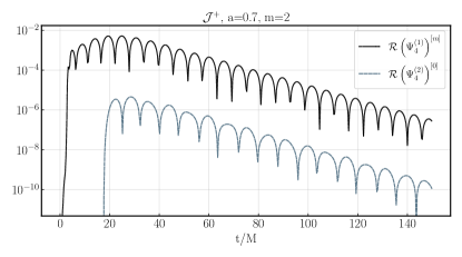
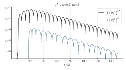
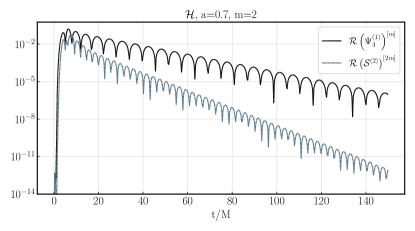
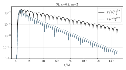
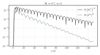
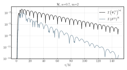
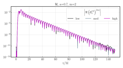
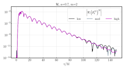
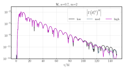
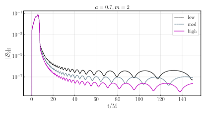
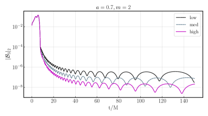
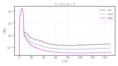
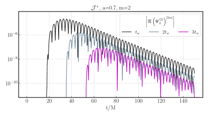
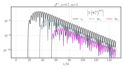
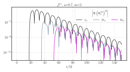
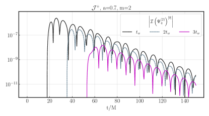
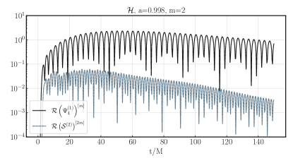
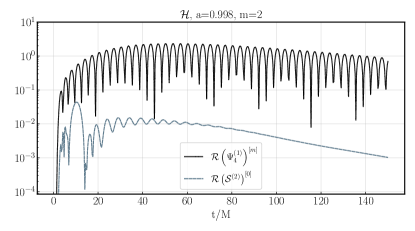
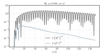
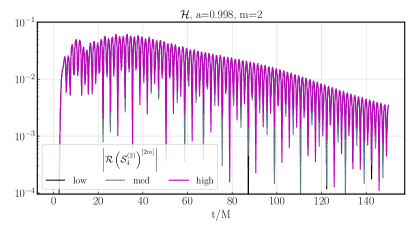
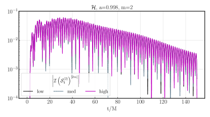
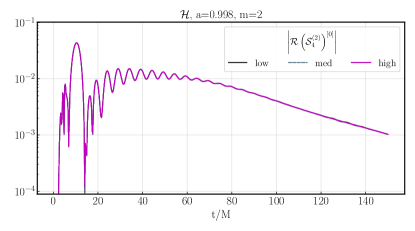
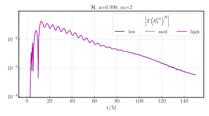
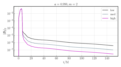
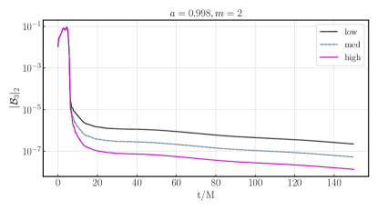
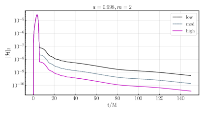
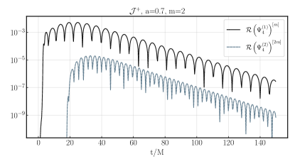
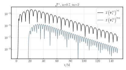
In Fig. 2 we plot the absolute value of the real and imaginary parts of Ψ4(1),[m]superscriptsubscriptΨ41delimited-[]𝑚\Psi_{4}^{(1),[m]}, along with Ψ4(2),[2m]superscriptsubscriptΨ42delimited-[]2𝑚\Psi_{4}^{(2),[2m]} and Ψ4(2),[0]superscriptsubscriptΨ42delimited-[]0\Psi_{4}^{(2),[0]}, measured at future null infinity. The time offset between the start of the first and second order components of the waveform is due to the delayed integration start time Twsubscript𝑇𝑤T_{w} of the latter compared to the former; T=Tw𝑇subscript𝑇𝑤T=T_{w} is twice the earliest time we can begin the second order evolution with a consistent source term. In Fig. 3 we plot the absolute value of the real and imaginary parts of Ψ4(1)superscriptsubscriptΨ41\Psi_{4}^{(1)} and 𝒮(2)superscript𝒮2\mathcal{S}^{(2)} on the black hole horizon; Fig. 4 shows a resolution study of the latter. The region near the horizon is where the source term is most significant (it decays faster than 1/r1𝑟1/r going to null infinity), and as expected 𝒮(2)(Ψ4(1))2similar-tosuperscript𝒮2superscriptsuperscriptsubscriptΨ412\mathcal{S}^{(2)}\sim\left(\Psi_{4}^{(1)}\right)^{2} there. In Fig. 5 we plot norms of the metric reconstruction independent residuals discussed in Sec.V.8, at three different resolutions. After the constraint violating portions have left the domain, we find roughly exponential convergence to zero, in agreement with what one would expect from a pseudo-spectral code with a sufficiently small time step so that the time integration truncation error is subdominant.
Refer to caption
(a) ψ4(1)[2]superscriptsubscript𝜓41delimited-[]2\mathcal{R}\psi_{4}^{(1)[2]}, ψ4(2)[4]superscriptsubscript𝜓42delimited-[]4\mathcal{R}\psi_{4}^{(2)[4]}
Refer to caption
(b) ψ4(1)[2]superscriptsubscript𝜓41delimited-[]2\mathcal{I}\psi_{4}^{(1)[2]}, ψ4(2)[4]superscriptsubscript𝜓42delimited-[]4\mathcal{I}\psi_{4}^{(2)[4]}
Refer to caption
(c) ψ4(1)[2]superscriptsubscript𝜓41delimited-[]2\mathcal{R}\psi_{4}^{(1)[2]}, ψ4(2)[0]superscriptsubscript𝜓42delimited-[]0\mathcal{R}\psi_{4}^{(2)[0]}
Refer to caption
(d) ψ4(1)[2]superscriptsubscript𝜓41delimited-[]2\mathcal{I}\psi_{4}^{(1)[2]}, ψ4(2)[0]superscriptsubscript𝜓42delimited-[]0\mathcal{I}\psi_{4}^{(2)[0]}
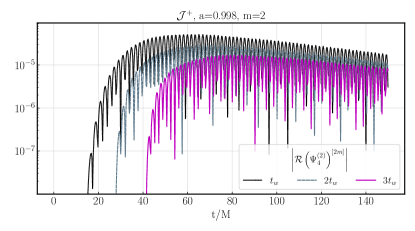
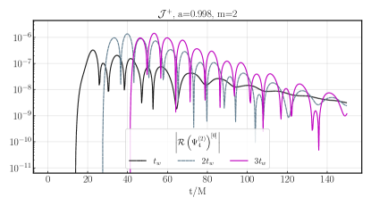
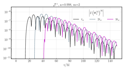
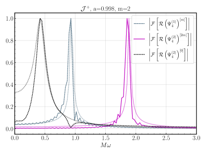
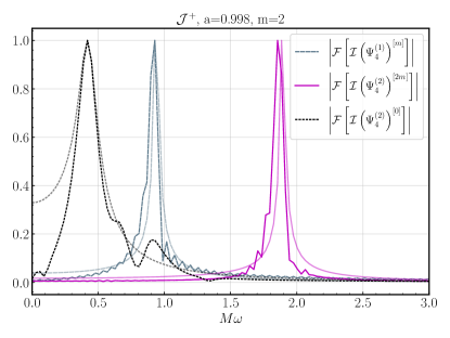
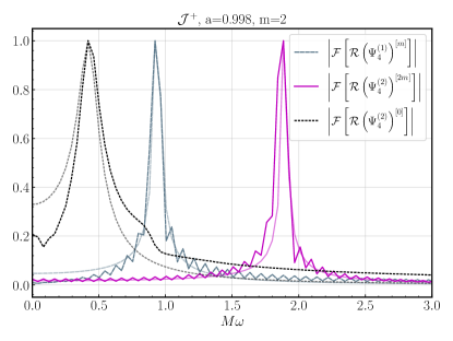
Figure 2: Behavior of the real (left) and imaginary (right) parts of r×Ψ4(1),[m]𝑟superscriptsubscriptΨ41delimited-[]𝑚r\times\Psi_{4}^{(1),[m]} (here m=2𝑚2m=2) at future null infinity (𝒥+superscript𝒥\mathcal{J}^{+}), compared with r×Ψ4(2),[2m]𝑟superscriptsubscriptΨ42delimited-[]2𝑚r\times\Psi_{4}^{(2),[2m]} (top) and r×Ψ4(2),[0]𝑟superscriptsubscriptΨ42delimited-[]0r\times\Psi_{4}^{(2),[0]} (bottom), for the a=0.7𝑎0.7a=0.7 case (see Table. 3 for simulation parameters). For reference we show the same Ψ4(1)superscriptsubscriptΨ41\Psi_{4}^{(1)} data in the top and bottom panel for each case, though notice the different vertical scales. Ψ4(1)superscriptsubscriptΨ41\Psi_{4}^{(1)} is initially zero as the data is compactly supported near the origin, and Ψ4(2)superscriptsubscriptΨ42\Psi_{4}^{(2)} is zero until we begin its evolution at Tw=17.6Msubscript𝑇𝑤17.6𝑀T_{w}=17.6M; see Fig. 6 for results with this turn-on time delayed to 2Tw2subscript𝑇𝑤2T_{w} and 3Tw3subscript𝑇𝑤3T_{w}. The data is from the ‘high’ resolution run, and the truncation error estimate for all these functions remains 1%less-than-or-similar-toabsentpercent1\lesssim 1\% throughout the evolution.
Refer to caption
(a) ψ4(1)[2]superscriptsubscript𝜓41delimited-[]2\mathcal{R}\psi_{4}^{(1)[2]}, 𝒮[4]superscript𝒮delimited-[]4\mathcal{R}\mathcal{S}^{[4]}
Refer to caption
(b) ψ4(1)[2]superscriptsubscript𝜓41delimited-[]2\mathcal{I}\psi_{4}^{(1)[2]}, 𝒮[4]superscript𝒮delimited-[]4\mathcal{I}\mathcal{S}^{[4]}
Refer to caption
(c) ψ4(1)[2]superscriptsubscript𝜓41delimited-[]2\mathcal{R}\psi_{4}^{(1)[2]}, 𝒮[0]superscript𝒮delimited-[]0\mathcal{R}\mathcal{S}^{[0]}
Refer to caption
(d) ψ4(1)[2]superscriptsubscript𝜓41delimited-[]2\mathcal{I}\psi_{4}^{(1)[2]}, 𝒮[0]superscript𝒮delimited-[]0\mathcal{I}\mathcal{S}^{[0]}
Figure 3: Comparison of the magnitude of the real (left) and imaginary (right) components of Ψ4(1)superscriptsubscriptΨ41\Psi_{4}^{(1)} with the corresponding components of the second order source terms for 𝒮(2),[4]superscript𝒮2delimited-[]4\mathcal{S}^{(2),[4]} (top) and 𝒮(2),[0]superscript𝒮2delimited-[]0\mathcal{S}^{(2),[0]} (bottom), at the black hole horizon, for the a=0.7𝑎0.7a=0.7 case (Table  3). For reference we show the same Ψ4(1)superscriptsubscriptΨ41\Psi_{4}^{(1)} data in the top and bottom panel for each case.
Refer to caption
(a) 𝒮[4]superscript𝒮delimited-[]4\mathcal{R}\mathcal{S}^{[4]}
Refer to caption
(b) 𝒮[4]superscript𝒮delimited-[]4\mathcal{I}\mathcal{S}^{[4]}
Refer to caption
(c) 𝒮[0]superscript𝒮delimited-[]0\mathcal{R}\mathcal{S}^{[0]}
Refer to caption
(d) 𝒮[0]superscript𝒮delimited-[]0\mathcal{I}\mathcal{S}^{[0]}
Figure 4: A resolution study of the real (left) and imaginary (right) parts of the second order source terms 𝒮(2)[4]superscript𝒮2delimited-[]4\mathcal{S}^{(2)[4]} (top) and 𝒮(2)[0]superscript𝒮2delimited-[]0\mathcal{S}^{(2)[0]} (bottom) at the black hole horizon, for the a=0.7𝑎0.7a=0.7 case (Table  3). This demonstrates that we are resolving the source terms until relatively late times (t/M120similar-to𝑡𝑀120t/M\sim 120 at high resolution).
Refer to caption
(a) |2|2subscriptsubscript22\left|\mathcal{B}_{2}\right|_{2}
Refer to caption
(b) |3|2subscriptsubscript32\left|\mathcal{B}_{3}\right|_{2}
Refer to caption
(c) ||2subscript2\left|\mathcal{H}\right|_{2}
Figure 5: The discrete two norm (see Eq. (A)) of independent residuals 3subscript3\mathcal{B}_{3}, 2subscript2\mathcal{B}_{2}, and \mathcal{H} for metric reconstruction (see respectively Eq. (V.8), Eq. (V.8), and Eq. (44)), for the spin a=0.7𝑎0.7a=0.7 case, as a function of time for three different resolutions (Table. 3). We only begin to obtain convergence to zero once the region with inconsistent initial data has left our computational domain (around t/M10similar-to𝑡𝑀10t/M\sim 10).

Though this initial data is more to illustrate our solution scheme and is not astrophysically accurate, it is useful to begin to understand the non-linear response when the black hole is excited by the fundamental l=m=2𝑙𝑚2l=m=2 quasinormal mode, in particular if we wait a sufficiently long time for overtones present in the initial data to decay888In a Kerr spacetime, setting initial data (38) with a single l0subscript𝑙0l_{0} mode of the spin-weighted Legendre polynomials Pl0mssubscriptsubscriptsuperscript𝑃𝑚subscript𝑙0𝑠{}_{s}P^{m}_{l_{0}} will excite a spectrum of different l𝑙l quasinormal modes measured at infinity, unless the black hole spin a=0𝑎0a=0.. Fig. 2 suggests T=Tw𝑇subscript𝑇𝑤T=T_{w} might not be early enough, as Ψ4(1)superscriptsubscriptΨ41\Psi_{4}^{(1)} has just started to enter its decaying phase. In Fig. 6 then we show results for the second order modes with the evolution begun at 2Tw2subscript𝑇𝑤2T_{w} and 3Tw3subscript𝑇𝑤3T_{w}, in addition to Twsubscript𝑇𝑤T_{w} depicted in Fig. 2. The later start times show qualitatively similar behavior, except the amplitude is lower by a factor close to the square of the decay in the amplitude of Ψ4(1)superscriptsubscriptΨ41\Psi_{4}^{(1)} over the relevant delay time. To help interpret the results further, in Fig. 7 we plot the normalized absolute value of the Fourier transform of Ψ4subscriptΨ4\Psi_{4}, taken with two different windows: an earlier time window to capture the prompt second order response (but still sufficiently past T=0𝑇0T=0 that the first order source is dominated by the single decaying quasinormal mode), and a later time window to show the late time behavior once second order transient effects have decayed. Also shown for reference are Fourier transforms of pure damped sinusoids corresponding to the dominant fundamental quasinormal modes expected for each m𝑚m.

Refer to caption
(a) ψ4(2)[4]superscriptsubscript𝜓42delimited-[]4\mathcal{R}\psi_{4}^{(2)[4]}
Refer to caption
(b) ψ4(2)[4]superscriptsubscript𝜓42delimited-[]4\mathcal{I}\psi_{4}^{(2)[4]}
Refer to caption
(c) ψ4(2)[0]superscriptsubscript𝜓42delimited-[]0\mathcal{R}\psi_{4}^{(2)[0]}
Refer to caption
(d) ψ4(2)[0]superscriptsubscript𝜓42delimited-[]0\mathcal{I}\psi_{4}^{(2)[0]}
Figure 6: Comparison of the real (left) and imaginary (right) components of the second order Ψ4(2),[4]superscriptsubscriptΨ42delimited-[]4\Psi_{4}^{(2),[4]} (top) and Ψ4(2),[0]superscriptsubscriptΨ42delimited-[]0\Psi_{4}^{(2),[0]} (bottom) fields, from the same a=0.7𝑎0.7a=0.7 first order perturbation depicted in Fig. 2, as a function of when we begin evolving the second order field. Three cases are shown, including for reference the Twsubscript𝑇𝑤T_{w} case also shown in Fig. 2.
Refer to caption
(a) \mathcal{F}\mathcal{R}, window (53M,150M)53𝑀150𝑀(53M,150M)
Refer to caption
(b) \mathcal{F}\mathcal{I}, window (53M,150M)53𝑀150𝑀(53M,150M)
Refer to caption
(c) \mathcal{F}\mathcal{R}, window (88M,150M)88𝑀150𝑀(88M,150M)
Refer to caption
(d) \mathcal{F}\mathcal{I}, window (88M,150M)88𝑀150𝑀(88M,150M)
Figure 7: Normalized absolute value of the Fourier Transform (48) of the real (left) and imaginary (right) parts of Ψ4(1),[2]superscriptsubscriptΨ41delimited-[]2\Psi_{4}^{(1),[2]}, Ψ4(2),[4]superscriptsubscriptΨ42delimited-[]4\Psi_{4}^{(2),[4]}, and Ψ4(2),[0]superscriptsubscriptΨ42delimited-[]0\Psi_{4}^{(2),[0]}, taken over two different windows, for the a=0.7𝑎0.7a=0.7 case (see Table 3). The data for the second order components come from the 3Tw3subscript𝑇𝑤3T_{w} start time (see Fig.6). The window for the top panels is from [3Tw,150M]3subscript𝑇𝑤150𝑀[3T_{w},150M], thus including the early time behavior of the response, while for the bottom panels is [5Tw,150M]5subscript𝑇𝑤150𝑀[5T_{w},150M] to focus on the late time response. The darker plotted lines are from the numerical output, while the lighter plotted lines are the Fourier transform of eωItsin(ωRt)superscript𝑒subscript𝜔𝐼𝑡sinsubscript𝜔𝑅𝑡e^{-\omega_{I}t}\mathrm{sin}\left(\omega_{R}t\right) with damping time 1/ωI1subscript𝜔𝐼1/\omega_{I} and frequency ωRsubscript𝜔𝑅\omega_{R} of the l=m𝑙𝑚l=m (e.g. l=2,m=2formulae-sequence𝑙2𝑚2l=2,m=2) quasinormal mode for an a=0.7𝑎0.7a=0.7 spin black hole computed via Leaver’s method (taken from Berti et al. (2009)).

These plots illustrate a couple of interesting aspects of the second order piece of a quasinormal mode perturbation of an a=0.7𝑎0.7a=0.7 spin Kerr black hole. First, beginning with zero initial data for Ψ4(2)superscriptsubscriptΨ42\Psi_{4}^{(2)} on our T=const.𝑇constT={\rm const.} slice, the response at future null infinity builds up to a maximum over 1-2 local dynamical times scales, before settling down to a quasinormal mode-like decay. This is in part because where the source term is most significant is spread out over a region a few Schwarzschild radii about the horizon, and in part because of our prompt start of the second order evolution. Second, the source term clearly excites the fundamental m=0𝑚0m=0 and m=4𝑚4m=4 quasinormal modes (i.e. solutions one would obtain from the source-free Teukolsky equation), and these dominate the late time response due to their slower decay. Or said another way, suppose the late time response was purely a driven mode, then (following the behavior of the source term in Fig. 3) one would expect the slope to be twice that of the first order mode, and the amplitude of the second order piece at a given late-time should not depend on the start time, unlike what is shown in Figs. 2 and 6.999All this behavior can qualitatively be captured by a driven, damped harmonic oscillator model, d2y(t)/dt2+λdy(t)/dt+ω2y(t)=f(t)superscript𝑑2𝑦𝑡𝑑superscript𝑡2𝜆𝑑𝑦𝑡𝑑𝑡superscript𝜔2𝑦𝑡𝑓𝑡d^{2}y(t)/dt^{2}+\lambda\ dy(t)/dt+\omega^{2}\ y(t)=f(t), where the source f(t)𝑓𝑡f(t) is zero before being turned on at time t0subscript𝑡0t_{0}. In addition to the driven (particular solution) response to f(t)𝑓𝑡f(t), demanding continuity in y𝑦y and dy/dt𝑑𝑦𝑑𝑡dy/dt at t=t0𝑡subscript𝑡0t=t_{0} will generically require that the fundamental modes (homogeneous solutions) of the oscillator are also excited then. From the perspective of the Fourier transforms in Fig. 7, for m=4𝑚4m=4 the presence of this early time behavior can be inferred by the narrower shape of the numerical data curve compared to that of the fundamental quasinormal mode: the driven and fundamental modes have essentially the same frequency to within the resolution of the Fourier transform here, and despite the more rapid decay of the former, the initial growth phase (Fig. 6) makes the transform of their sum look slightly closer to that of an undamped sinusoid (a delta function). The interpretation of the m=0𝑚0m=0 mode in this sense is less clear.

An implication of the above for ringdown studies are (caveats about the physical accuracy of our initial data aside): if an l=m=4𝑙𝑚4l=m=4 component is searched for following a comparable mass merger, given this mode’s low amplitude relative to the l=m=2𝑙𝑚2l=m=2 mode, in the first few cycles of ringdown non-linear energy transfer from the l=m=2𝑙𝑚2l=m=2 to the l=m=4𝑙𝑚4l=m=4 mode could be observable and should be accounted for. Furthermore, once past this and in the linear regime, the amplitude and phase of the l=m=4𝑙𝑚4l=m=4 mode that may be measured then would differ from the linear evolution of what one could consider as the “initial” amplitude and phase of this mode excited by merger. With proposals to coherently stack multiple detected events to search for common subdominant modes that rely on knowledge of predicted amplitudes and phases Yang et al. (2017), this implies non-linear effects need to be accounted for, either by incorporating them in the models, or using the “final” amplitudes and phases if only the linear portion of the waveforms are included.

VI.2 Example evolution with black hole spin a=0.998𝑎0.998a=0.998

Here we show results from a simulation of the perturbation of a black hole with a spin near the “Thorne limit” Thorne (1974) a0.998similar-to𝑎0.998a\sim 0.998, which is expected to be the maximum black hole spin that can be achieved within a class of thin-disk accretion models. Our simulation parameters are listed in Table. 4. Note that the relevant dynamical timescale for a near extremal black hole is TdM/1asimilar-tosubscript𝑇𝑑𝑀1𝑎T_{d}\sim M/\sqrt{1-a}. For a=0.998𝑎0.998a=0.998, Td22Msimilar-tosubscript𝑇𝑑22𝑀T_{d}\sim 22M, so evolving for T150Msimilar-to𝑇150𝑀T\sim 150M corresponds to T7×Tdsimilar-to𝑇7subscript𝑇𝑑T\sim 7\times T_{d}, a considerably shorter time in terms of Tdsubscript𝑇𝑑T_{d} than for a=0.7𝑎0.7a=0.7. Given that it is computationally intensive to evolve the a=0.998𝑎0.998a=0.998 case for a comparable number of dynamical timescales with our present code, we leave investigating late time effects to future work.

mass 0.50.50.5
spin 0.4990.4990.499 (a=0.998𝑎0.998a=0.998)
low resolution Nx=176subscript𝑁𝑥176N_{x}=176, Nl=32subscript𝑁𝑙32N_{l}=32
med resolution Nx=192subscript𝑁𝑥192N_{x}=192, Nl=36subscript𝑁𝑙36N_{l}=36
high resolution Nx=208subscript𝑁𝑥208N_{x}=208, Nl=40subscript𝑁𝑙40N_{l}=40
Twsubscript𝑇𝑤T_{w} 2×Tmw13.6M2subscript𝑇𝑚𝑤13.6𝑀2\times T_{mw}\approx 13.6M
m𝑚m 22-2
l0subscript𝑙0l_{0} 222
a0subscript𝑎0a_{0} 0.10.10.1
rusubscript𝑟𝑢r_{u} 1.1×rH1.1subscript𝑟𝐻1.1\times r_{H}
rlsubscript𝑟𝑙r_{l} 2.5×rH2.5subscript𝑟𝐻2.5\times r_{H}
Table 4: Parameters for spin a=0.998𝑎0.998a=0.998 black hole evolution (unless stated otherwise in the figure captions). Twsubscript𝑇𝑤T_{w} is the “wait” time before starting the evolution of Ψ4(2)superscriptsubscriptΨ42\Psi_{4}^{(2)}, which we choose to be twice the “minimum” wait time Tmwsubscript𝑇𝑚𝑤T_{mw} for the initial data we choose; see Sec. (IV).

We show the same set of data as from the a=0.7𝑎0.7a=0.7 runs : the magnitudes of Ψ4(1)superscriptsubscriptΨ41\Psi_{4}^{(1)} and Ψ4(2)superscriptsubscriptΨ42\Psi_{4}^{(2)} at future null infinity (Fig.8), the magnitudes of Ψ4(1)superscriptsubscriptΨ41\Psi_{4}^{(1)} and 𝒮(2)superscript𝒮2\mathcal{S}^{(2)} at the horizon (Fig.9), a resolution study of the latter (Fig. 10), convergence of the metric reconstruction independent residuals (Fig.11), the second order response with varied start time (Fig.12), and Fourier transforms of Ψ4(1)superscriptsubscriptΨ41\Psi_{4}^{(1)} and Ψ4(2)superscriptsubscriptΨ42\Psi_{4}^{(2)} at future null infinity (Fig.13).
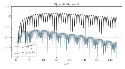
Refer to caption
(a) ψ4(1)[2]superscriptsubscript𝜓41delimited-[]2\mathcal{R}\psi_{4}^{(1)[2]}, ψ4(2)[4]superscriptsubscript𝜓42delimited-[]4\mathcal{R}\psi_{4}^{(2)[4]}
Refer to caption
(b) ψ4(1)[2]superscriptsubscript𝜓41delimited-[]2\mathcal{I}\psi_{4}^{(1)[2]}, ψ4(2)[4]superscriptsubscript𝜓42delimited-[]4\mathcal{I}\psi_{4}^{(2)[4]}
Refer to caption
(c) ψ4(1)[2]superscriptsubscript𝜓41delimited-[]2\mathcal{R}\psi_{4}^{(1)[2]}, ψ4(2)[0]superscriptsubscript𝜓42delimited-[]0\mathcal{R}\psi_{4}^{(2)[0]}
Refer to caption
(d) ψ4(1)[2]superscriptsubscript𝜓41delimited-[]2\mathcal{I}\psi_{4}^{(1)[2]}, ψ4(2)[0]superscriptsubscript𝜓42delimited-[]0\mathcal{I}\psi_{4}^{(2)[0]}
Figure 8: Behavior of the real (left) and imaginary (right) parts of r×Ψ4(1),[m]𝑟superscriptsubscriptΨ41delimited-[]𝑚r\times\Psi_{4}^{(1),[m]} (here m=2𝑚2m=2) at future null infinity (𝒥+superscript𝒥\mathcal{J}^{+}), compared with r×Ψ4(2),[2m]𝑟superscriptsubscriptΨ42delimited-[]2𝑚r\times\Psi_{4}^{(2),[2m]} (top) and r×Ψ4(2),[0]𝑟superscriptsubscriptΨ42delimited-[]0r\times\Psi_{4}^{(2),[0]} (bottom), for the a=0.998𝑎0.998a=0.998 case (see Table. 4 for simulation parameters). As with the data shown for the a=0.7𝑎0.7a=0.7 case in Fig.2, the truncation error estimates are less than 1%similar-toabsentpercent1\sim 1\% throughout.
Refer to caption
(a) ψ4(1)[2]superscriptsubscript𝜓41delimited-[]2\mathcal{R}\psi_{4}^{(1)[2]}, 𝒮[4]superscript𝒮delimited-[]4\mathcal{R}\mathcal{S}^{[4]}
Refer to caption
(b) ψ4(1)[2]superscriptsubscript𝜓41delimited-[]2\mathcal{I}\psi_{4}^{(1)[2]}, 𝒮[4]superscript𝒮delimited-[]4\mathcal{I}\mathcal{S}^{[4]}
Refer to caption
(c) ψ4(1)[2]superscriptsubscript𝜓41delimited-[]2\mathcal{R}\psi_{4}^{(1)[2]}, 𝒮[0]superscript𝒮delimited-[]0\mathcal{R}\mathcal{S}^{[0]}
Refer to caption
(d) ψ4(1)[2]superscriptsubscript𝜓41delimited-[]2\mathcal{I}\psi_{4}^{(1)[2]}, 𝒮[0]superscript𝒮delimited-[]0\mathcal{I}\mathcal{S}^{[0]}
Figure 9: Comparison of the magnitude of the real (left) and imaginary (right) components of Ψ4(1)superscriptsubscriptΨ41\Psi_{4}^{(1)} with the corresponding components of the second order source terms for 𝒮(2),[4]superscript𝒮2delimited-[]4\mathcal{S}^{(2),[4]} (top) and 𝒮(2),[0]superscript𝒮2delimited-[]0\mathcal{S}^{(2),[0]} (bottom), at the black hole horizon, for the a=0.998𝑎0.998a=0.998 case (Table  3).
Refer to caption
(a) 𝒮[4]superscript𝒮delimited-[]4\mathcal{R}\mathcal{S}^{[4]}
Refer to caption
(b) 𝒮[4]superscript𝒮delimited-[]4\mathcal{I}\mathcal{S}^{[4]}
Refer to caption
(c) 𝒮[0]superscript𝒮delimited-[]0\mathcal{R}\mathcal{S}^{[0]}
Refer to caption
(d) 𝒮[0]superscript𝒮delimited-[]0\mathcal{I}\mathcal{S}^{[0]}
Figure 10: A resolution study of the real (left) and imaginary (right) parts of the second order source terms 𝒮(2)[4]superscript𝒮2delimited-[]4\mathcal{S}^{(2)[4]} (top) and 𝒮(2)[0]superscript𝒮2delimited-[]0\mathcal{S}^{(2)[0]} (bottom) at the black hole horizon, for the a=0.998𝑎0.998a=0.998 case (Table  4). This demonstrates that we are resolving the source terms over the entire integration time (T=0,150M𝑇0150𝑀T=0,150M).
Refer to caption
(a) |2|2subscriptsubscript22\left|\mathcal{B}_{2}\right|_{2}
Refer to caption
(b) |3|2subscriptsubscript32\left|\mathcal{B}_{3}\right|_{2}
Refer to caption
(c) ||2subscript2\left|\mathcal{H}\right|_{2}
Figure 11: The discrete two norm (see Eq. (A)) of independent residuals 3subscript3\mathcal{B}_{3}, 2subscript2\mathcal{B}_{2}, and \mathcal{H} for metric reconstruction (see respectively Eq. (V.8), Eq. (V.8), and Eq. (44)), for the spin a=0.998𝑎0.998a=0.998 case, as a function of time for three different resolutions (Table. 4). We only begin to obtain convergence to zero once the region with inconsistent initial data has left our computational domain (around t/M5similar-to𝑡𝑀5t/M\sim 5).
Refer to caption
(a) ψ4(2)[4]superscriptsubscript𝜓42delimited-[]4\mathcal{R}\psi_{4}^{(2)[4]}
Refer to caption
(b) ψ4(2)[4]superscriptsubscript𝜓42delimited-[]4\mathcal{I}\psi_{4}^{(2)[4]}
Refer to caption
(c) ψ4(2)[0]superscriptsubscript𝜓42delimited-[]0\mathcal{R}\psi_{4}^{(2)[0]}
Refer to caption
(d) ψ4(2)[0]superscriptsubscript𝜓42delimited-[]0\mathcal{I}\psi_{4}^{(2)[0]}
Figure 12: Comparison of the real (left) and imaginary (right) components of the second order Ψ4(2),[4]superscriptsubscriptΨ42delimited-[]4\Psi_{4}^{(2),[4]} (top) and Ψ4(2),[0]superscriptsubscriptΨ42delimited-[]0\Psi_{4}^{(2),[0]} (bottom) fields, from the same a=0.998𝑎0.998a=0.998 first order perturbation depicted in Fig. 8, as a function of when we begin evolving the second order field. Three cases are shown, including for reference the Twsubscript𝑇𝑤T_{w} case also shown in Fig. 8.
Refer to caption
(a) \mathcal{F}\mathcal{R}, window (41M,95M)41𝑀95𝑀(41M,95M)
Refer to caption
(b) \mathcal{F}\mathcal{I}, window (41M,95M)41𝑀95𝑀(41M,95M)
Refer to caption
(c) \mathcal{F}\mathcal{R}, window (68M,150M)68𝑀150𝑀(68M,150M)
Refer to caption
(d) \mathcal{F}\mathcal{I}, window (68M,150M)68𝑀150𝑀(68M,150M)
Figure 13: Normalized absolute value of the Fourier Transform (48) of the real (left) and imaginary (right) parts of Ψ4(1),[2]superscriptsubscriptΨ41delimited-[]2\Psi_{4}^{(1),[2]}, Ψ4(2),[4]superscriptsubscriptΨ42delimited-[]4\Psi_{4}^{(2),[4]}, and Ψ4(2),[0]superscriptsubscriptΨ42delimited-[]0\Psi_{4}^{(2),[0]}, taken over two different windows, for the a=0.998𝑎0.998a=0.998 case (see Table 4). As in Fig.7 for the a=0.7𝑎0.7a=0.7 case, the data for the second order components come from the 3Tw3subscript𝑇𝑤3T_{w} start time (see Fig.12), the top (bottom) panels use a [3Tw,150M]3subscript𝑇𝑤150𝑀[3T_{w},150M] ([5Tw,150M]5subscript𝑇𝑤150𝑀[5T_{w},150M]) window, darker lines are from the numerical output, and the lighter lines are the Fourier transforms of the corresponding quasinormal modes of a spin a=0.998𝑎0.998a=0.998 black hole. The small angular oscillations in the measured Fourier transforms are due to our (Dirichlet) windowing of the measured waveform.

For the most part the interpretation of the results is similar to the a=0.7𝑎0.7a=0.7 case, taking into account the shorter evolution time in terms of Tdsubscript𝑇𝑑T_{d} for the a=0.998𝑎0.998a=0.998 case. A notable difference though is a significant non-oscillatory component to the second order m=0𝑚0m=0 mode. One can roughly understand why such a component might appear given our initial data for Ψ4(1),[m]eiωRtωItproportional-tosuperscriptsubscriptΨ41delimited-[]𝑚superscript𝑒𝑖subscript𝜔𝑅𝑡subscript𝜔𝐼𝑡\Psi_{4}^{(1),[m]}\propto e^{i\omega_{R}t-\omega_{I}t} (we follow the quasinormal mode convention where an exponential eiωtsuperscript𝑒𝑖𝜔𝑡e^{i\omega t} has complex frequency ωωR+iωI𝜔subscript𝜔𝑅𝑖subscript𝜔𝐼\omega\equiv\omega_{R}+i\omega_{I}). The m=0𝑚0m=0 source term largely comes form reconstructed fields of the form p[m]×q[m]¯superscript𝑝delimited-[]𝑚¯superscript𝑞delimited-[]𝑚p^{[m]}\times\overline{q^{[m]}}, where p[m],q[m]Ψ4(1),[m]proportional-tosuperscript𝑝delimited-[]𝑚superscript𝑞delimited-[]𝑚superscriptsubscriptΨ41delimited-[]𝑚p^{[m]},q^{[m]}\propto\Psi_{4}^{(1),[m]}; hence their oscillatory components can cancel, leaving a real exponential piece decaying at roughly twice the rate of Ψ4(1),[m]superscriptsubscriptΨ41delimited-[]𝑚\Psi_{4}^{(1),[m]}. For near extremal spins (in contrast to the a=0.7𝑎0.7a=0.7 case), this driven component has a decay rate quite close to the fundamental m=0,l=2formulae-sequence𝑚0𝑙2m=0,l=2 harmonic 101010See e.g. Table II of Berti et al. (2006) for their a=0.98𝑎0.98a=0.98 case, the closest spin to our value that they list., which is why it remains visible in the waveform at late times. We find that how much of an oscillatory vs pure exponential piece is visible in either of the real or imaginary parts of Ψ4(2),[0]superscriptsubscriptΨ42delimited-[]0\Psi_{4}^{(2),[0]} depends quite sensitively on the relative amplitudes and phases of the real vs imaginary components of Ψ4(1)superscriptsubscriptΨ41\Psi_{4}^{(1)} in the initial data.

VII Conclusion and further extensions

We have presented a new numerical evolution scheme to reconstruct the linear metric from the Weyl scalar Ψ4(1)superscriptsubscriptΨ41\Psi_{4}^{(1)} in Kerr spacetimes, along with a numerical implementation of the equations of motion for the second order perturbation Ψ4(2)superscriptsubscriptΨ42\Psi_{4}^{(2)} (a more detailed discussion of the analytic framework we used is discussed in the Appendices of this paper, and in our first paper Loutrel et al. (2020)). This first implementation is limited in several respects, and in the remainder of this section we outline possible extensions that will allow more direct application to our desired goals of studying second order effects in post-merger black hole ringdown, investigating gravitational wave turbulence, and other related issues for rapidly rotating Kerr black holes.

In this study we only considered mode coupling from a single mode of angular number m𝑚m, Ψ4(1),[m]superscriptsubscriptΨ41delimited-[]𝑚\Psi_{4}^{(1),[m]}, to produce the frequency doubled second order components Ψ4(2),[2m]superscriptsubscriptΨ42delimited-[]2𝑚\Psi_{4}^{(2),[2m]} and Ψ4(2),[0]superscriptsubscriptΨ42delimited-[]0\Psi_{4}^{(2),[0]}. Astrophysically realistic sets of initial data will include many different modes, and the second order perturbations for an m𝑚m mode will be a sum over all modes (m1,m2)subscript𝑚1subscript𝑚2(m_{1},m_{2}) such that m1+m2=msubscript𝑚1subscript𝑚2𝑚m_{1}+m_{2}=m. We leave exploring such more complicated mode mixing to future work.

Constructing astrophysically realistic initial data for Ψ4(1)superscriptsubscriptΨ41\Psi_{4}^{(1)}, and the l=0,1𝑙01l=0,1 components of the metric and NP scalars that represent the changes in mass and spin corresponding to the given Ψ4(1)superscriptsubscriptΨ41\Psi_{4}^{(1)}, remain unsolved problems in black hole perturbation theory. This will require specifying a Ψ4(1)superscriptsubscriptΨ41\Psi_{4}^{(1)} that matches a desired scenario at T=0𝑇0T=0, and then solving a set of constraint equations to give consistent initial conditions (perturbed metric and related NP quantities) for the reconstruction transport equations. These constraint equations are most naturally expressed in terms of geometric quantities intrinsic to the spacelike hypersurface T=0𝑇0T=0, giving rise to the familiar Hamiltonian and momentum contraint equations. One approach to take could be based on solving these equations using established approaches Baumgarte and Shapiro (2010), and then transforming the solutions to initial conditions for our scheme. Following a merger, finding appropriate values of Ψ4(1)superscriptsubscriptΨ41\Psi_{4}^{(1)} (or equivalently choosing the free initial data for hμνsubscript𝜇𝜈h_{\mu\nu} in a traditional scheme) describing the perturbation of the remnant, is less well understood. One possible approach to tackle this is to follow the lines of earlier analytical studies, including the close limit approximation to comparable mass black hole mergers Price and Pullin (1994), or related work done for the EMRI problem Apte and Hughes (2019); Lim et al. (2019). Another approach might be to map the data from a constant time slice of a full numerical simulation to our coordinates, and try to extract a perturbation relative to the late time Kerr solution. (And we note that, as discussed in more detail in the companion paper Loutrel et al. (2020), our goal is not to simply “solve” for the post merger waveform to second order; numerical relativity can already give us the full nonlinear solution as accurately as computer resources allow. Rather, we want to be able to interpret ringdown studies in terms of quasinormal modes, which requires understanding the waveform at a quantitative level that the full “answer”, in terms of a waveform by itself, cannot give.)

Another area of future work we mention is to investigate whether one can adapt our scheme to a gauge condition that is less restrictive on matter/effective matter in the spacetime than the outgoing radiation gauge. For at present we cannot study (for example) the EMRI problem, where there is a matter source representing the small body, and we cannot reconstruct the second order metric corresponding to the second order piece of Ψ4subscriptΨ4\Psi_{4}. To list two potential ways forward, it may be possible to continue to work in a radiation gauge but evolve a “corrector tensor” to include matter fields as in Green et al. (2020), or to directly reconstruct the metric in a different gauge, as is done in Chandrasekhar (2002); Andersson et al. (2019).

We emphasize that we have implemented a form of “ordinary” perturbation theory (e.g. Bender and Orszag (2013)), based on expansion in the curvature (or equivalently the peturbed metric)

Ψ4=Ψ4(1)+Ψ4(2)+,subscriptΨ4superscriptsubscriptΨ41superscriptsubscriptΨ42\displaystyle\Psi_{4}=\Psi_{4}^{(1)}+\Psi_{4}^{(2)}+\cdots, (45)

where the corrections are solved order-by-order, and at each order the new correction is assumed smaller than the prior sum. Up to second order then, the only non-linear phenomena we can explore is mode-coupling. We mentioned one of our goals was to understand whether Kerr black holes could exhibit “turbulence”, though exactly what turbulence means in the case of black holes is a bit nebulous. Regardless, the authors of Yang et al. (2015); Green et al. (2014) who first suggested turbulence could be present in the 4D case argued it would be a more subtle effect than can be described by ordinary perturbation theory, or at least would require some “resumming” of many terms in the sum. Instead then, they proposed an alternative perturbative expansion to try to capture such effects at leading beyond-linear order, showing in a scalar field model that a kind of parametric instability resulted that might be able to drive a turbulent cascade. It is still unknown whether such an effect occurs for gravitational perturbations of Kerr, though mode coupling more along the lines of what we describe here has been seen in full numerical solutions of both perturbed 4D Kerr black holes East et al. (2014) and black holes in 5D AdS spacetime Bantilan et al. (2012). We leave it to future work for a more thorough comparison with full numerical results, as well as how close second order mode coupling, augmented with energy transfer between modes guided by measurements at null infinity mentioned in Sec. III, could come to describing a turbulent-like cascade of energy for rapidly spinning black holes.

Acknowledgements

We are grateful to Andrew Spiers and Adam Pound for sharing results of their calculations which confirmed our calculation of Eq. (51) (and which confirmed several errors in Eq. (A4) of Campanelli and Lousto (1999)), to Stefan Hollands for discussions on the metric reconstruction method described in Green et al. (2020), and to Scott Hughes and Richard Price for a helpful discussion on our project and earlier work on second order black hole perturbation theory. N.L. & F.P. acknowledge support from NSF grant PHY-1912171, the Simons Foundation, and the Canadian Institute for Advanced Research (CIFAR). E.G. acknowledges support from NSF grant DMS-2006741. The simulations presented in this article were performed on computational resources managed and supported by Princeton Research Computing, a consortium of groups including the Princeton Institute for Computational Science and Engineering (PICSciE) and the Office of Information Technology’s High Performance Computing Center and Visualization Laboratory at Princeton University.

Appendix A Conventions for discrete norms and Fourier transforms

As fields are typically complex in the NP formalism, the discrete two norm of a field f𝑓f at a time level n𝑛n is defined to be the sum

|f(tn)|2subscript𝑓subscript𝑡𝑛2absent\displaystyle|f(t_{n})|_{2}\equiv
(1NxNyi=1Nxj=1Ny(\displaystyle\bigg{(}\frac{1}{N_{x}N_{y}}\sum_{i=1}^{N_{x}}\sum_{j=1}^{N_{y}}\big{(} (f(tn,ri,ϑj))2superscript𝑓subscript𝑡𝑛subscript𝑟𝑖subscriptitalic-ϑ𝑗2\displaystyle\left(\mathcal{R}f(t_{n},r_{i},\vartheta_{j})\right)^{2}
+(f(tn,ri,ϑj))2))1/2.\displaystyle+\left(\mathcal{I}f(t_{n},r_{i},\vartheta_{j})\right)^{2}\big{)}\bigg{)}^{1/2}. (46)

Our conventions for the Fourier transform are

f^(ω)=𝑑teiωtf(t),^𝑓𝜔superscriptsubscriptdifferential-d𝑡superscript𝑒𝑖𝜔𝑡𝑓𝑡\displaystyle\hat{f}(\omega)=\int_{-\infty}^{\infty}dte^{-i\omega t}f(t),
f(t)=dω2πeiωtf^(ω).𝑓𝑡superscriptsubscript𝑑𝜔2𝜋superscript𝑒𝑖𝜔𝑡^𝑓𝜔\displaystyle f(t)=\int_{-\infty}^{\infty}\frac{d\omega}{2\pi}e^{i\omega t}\hat{f}(\omega). (47)

And we define a normalized Fourier transform by

𝒩f^(ω)1maxf^|f^(ω)|.𝒩^𝑓𝜔1max^𝑓^𝑓𝜔\displaystyle\mathcal{N}\hat{f}(\omega)\equiv\frac{1}{\mathrm{max}\hat{f}}|\hat{f}(\omega)|. (48)

For reference the absolute value of the Fourier transform of f(t)=Θ(t)eωItsin(ωRt)𝑓𝑡Θ𝑡superscript𝑒subscript𝜔𝐼𝑡sinsubscript𝜔𝑅𝑡f(t)=\Theta(t)e^{-\omega_{I}t}\mathrm{sin}\left(\omega_{R}t\right) is

|f^(ω)|=ωR(ωR2+ωI2ω2)2+4ωI2ω2.^𝑓𝜔subscript𝜔𝑅superscriptsuperscriptsubscript𝜔𝑅2superscriptsubscript𝜔𝐼2superscript𝜔224superscriptsubscript𝜔𝐼2superscript𝜔2\displaystyle\left|\hat{f}(\omega)\right|=\frac{\omega_{R}}{\sqrt{\left(\omega_{R}^{2}+\omega_{I}^{2}-\omega^{2}\right)^{2}+4\omega_{I}^{2}\omega^{2}}}. (49)

Appendix B Derivation of metric reconstruction equations and source term in the outgoing radiation gauge

B.1 Tetrad, gauge, and first order spin coefficients

We assume the background is type D, that the background tetrad has been chosen to set Ψ0=Ψ1=Ψ3=Ψ4=κ=σ=ν=λ=0subscriptΨ0subscriptΨ1subscriptΨ3subscriptΨ4𝜅𝜎𝜈𝜆0\Psi_{0}=\Psi_{1}=\Psi_{3}=\Psi_{4}=\kappa=\sigma=\nu=\lambda=0, the linearized tetrad is as in (11a), and we are using outgoing radiation gauge for the first order metric perturbation (9a). For the Kerr spacetime we can also rotate the background tetrad to set γ=0𝛾0\gamma=0 (see Sec. C), and we assume we have done this.

It is worth noting that the tetrad components of the metric perturbation (10a) are all scalars of definite spin and boost weight, which we catalogue in Table 5 (for the angular tetrad projections we list the spin and boost of their complex conjugates, which is what we mostly use).

scalar weight spin weight boost weight
hllsubscript𝑙𝑙h_{ll} {2,2}22\{2,2\} 00 222
hlm¯subscript𝑙¯𝑚h_{l\bar{m}} {0,2}02\{0,2\} 11-1 111
hm¯m¯subscript¯𝑚¯𝑚h_{\bar{m}\bar{m}} {2,2}22\{-2,2\} 22-2 00
Table 5: Nonzero contractions of the perturbed metric.

We can write the first order perturbed tetrad in terms of the background tetrad. Following Chrzanowski (1976) (see also Campanelli and Lousto (1999); Loutrel et al. (2020)) we have

lμ(1)=subscriptsuperscript𝑙1𝜇absent\displaystyle l^{(1)}_{\mu}= 12hllnμ,12subscript𝑙𝑙subscript𝑛𝜇\displaystyle\frac{1}{2}h_{ll}n_{\mu}, (50a)
nμ(1)=subscriptsuperscript𝑛1𝜇absent\displaystyle n^{(1)}_{\mu}= 0,0\displaystyle 0, (50b)
mμ(1)=subscriptsuperscript𝑚1𝜇absent\displaystyle m^{(1)}_{\mu}= hlmnμ12hmmm¯μ,subscript𝑙𝑚subscript𝑛𝜇12subscript𝑚𝑚subscript¯𝑚𝜇\displaystyle h_{lm}n_{\mu}-\frac{1}{2}h_{mm}\bar{m}_{\mu}, (50c)

which then immediately gives the expressions for the perturbed derivative operators listed in (11a).

With the above choices for the tetrad/gauge, we find the following first order corrections to the spin coefficients (for the more general version of these expressions, without the choice of ingoing radiation gauge and γ=0𝛾0\gamma=0, see Loutrel et al. (2020)):

κ(1)=superscript𝜅1absent\displaystyle\kappa^{(1)}= (D2ϵρ¯)hlm𝐷2italic-ϵ¯𝜌subscript𝑙𝑚\displaystyle\left(D-2\epsilon-\bar{\rho}\right)h_{lm}
12(δ2α¯2β+π¯+τ)hll,12𝛿2¯𝛼2𝛽¯𝜋𝜏subscript𝑙𝑙\displaystyle-\frac{1}{2}\left(\delta-2\bar{\alpha}-2\beta+\bar{\pi}+\tau\right)h_{ll}, (51a)
λ(1)=superscript𝜆1absent\displaystyle\lambda^{(1)}= 12(Δμ+μ¯)hm¯m¯,12Δ𝜇¯𝜇subscript¯𝑚¯𝑚\displaystyle-\frac{1}{2}\left(\Delta-\mu+\bar{\mu}\right)h_{\bar{m}\bar{m}}, (51b)
σ(1)=superscript𝜎1absent\displaystyle\sigma^{(1)}= 12(D2ϵ+2ϵ¯+ρρ¯)hmm12𝐷2italic-ϵ2¯italic-ϵ𝜌¯𝜌subscript𝑚𝑚\displaystyle\frac{1}{2}\left(D-2\epsilon+2\bar{\epsilon}+\rho-\bar{\rho}\right)h_{mm}
(π¯+τ)hlm,¯𝜋𝜏subscript𝑙𝑚\displaystyle-\left(\bar{\pi}+\tau\right)h_{lm}, (51c)
ϵ(1)=superscriptitalic-ϵ1absent\displaystyle\epsilon^{(1)}= 14(Δμ+μ¯)hll14Δ𝜇¯𝜇subscript𝑙𝑙\displaystyle-\frac{1}{4}\left(\Delta-\mu+\bar{\mu}\right)h_{ll}
14(δ2α¯+π¯+2τ)hlm¯14𝛿2¯𝛼¯𝜋2𝜏subscript𝑙¯𝑚\displaystyle-\frac{1}{4}\left(\delta-2\bar{\alpha}+\bar{\pi}+2\tau\right)h_{l\bar{m}}
+14(δ¯2α3π2τ¯)hlm,14¯𝛿2𝛼3𝜋2¯𝜏subscript𝑙𝑚\displaystyle+\frac{1}{4}\left(\bar{\delta}-2\alpha-3\pi-2\bar{\tau}\right)h_{lm}, (51d)
ρ(1)superscript𝜌1\displaystyle\rho^{(1)} =12μhll+12(δ¯2απ)hlmabsent12𝜇subscript𝑙𝑙12¯𝛿2𝛼𝜋subscript𝑙𝑚\displaystyle=\frac{1}{2}\mu h_{ll}+\frac{1}{2}\left(\bar{\delta}-2\alpha-\pi\right)h_{lm}
12(δ2α¯+π¯+2τ)hlm¯,12𝛿2¯𝛼¯𝜋2𝜏subscript𝑙¯𝑚\displaystyle-\frac{1}{2}\left(\delta-2\bar{\alpha}+\bar{\pi}+2\tau\right)h_{l\bar{m}}, (51e)
α(1)=superscript𝛼1absent\displaystyle\alpha^{(1)}= 14(Δ2μ+μ¯)hlm¯14Δ2𝜇¯𝜇subscript𝑙¯𝑚\displaystyle-\frac{1}{4}\left(\Delta-2\mu+\bar{\mu}\right)h_{l\bar{m}}
14(δ2α¯+π¯+τ)hm¯m¯,14𝛿2¯𝛼¯𝜋𝜏subscript¯𝑚¯𝑚\displaystyle-\frac{1}{4}\left(\delta-2\bar{\alpha}+\bar{\pi}+\tau\right)h_{\bar{m}\bar{m}}, (51f)
β(1)=superscript𝛽1absent\displaystyle\beta^{(1)}= 14(Δ+μ+2μ¯)hlm14Δ𝜇2¯𝜇subscript𝑙𝑚\displaystyle-\frac{1}{4}\left(\Delta+\mu+2\bar{\mu}\right)h_{lm}
+14(δ¯+2β¯πτ¯)hmm,14¯𝛿2¯𝛽𝜋¯𝜏subscript𝑚𝑚\displaystyle+\frac{1}{4}\left(\bar{\delta}+2\bar{\beta}-\pi-\bar{\tau}\right)h_{mm}, (51g)
π(1)=superscript𝜋1absent\displaystyle\pi^{(1)}= 12(Δ+μ¯)hlm¯12τhm¯m¯,12Δ¯𝜇subscript𝑙¯𝑚12𝜏subscript¯𝑚¯𝑚\displaystyle-\frac{1}{2}\left(\Delta+\bar{\mu}\right)h_{l\bar{m}}-\frac{1}{2}\tau h_{\bar{m}\bar{m}}, (51h)
τ(1)=superscript𝜏1absent\displaystyle\tau^{(1)}= 12(Δ+μ)hlm12πhmm.12Δ𝜇subscript𝑙𝑚12𝜋subscript𝑚𝑚\displaystyle\frac{1}{2}\left(\Delta+\mu\right)h_{lm}-\frac{1}{2}\pi h_{mm}. (51i)

The following perturbed NP scalars are zero

ν(1)=γ(1)=μ(1)=0.superscript𝜈1superscript𝛾1superscript𝜇10\displaystyle\nu^{(1)}=\gamma^{(1)}=\mu^{(1)}=0. (52)

Notice that

π(1)+τ¯(1)=superscript𝜋1superscript¯𝜏1absent\displaystyle\pi^{(1)}+\bar{\tau}^{(1)}= 12(π¯+τ)hm¯m¯.12¯𝜋𝜏subscript¯𝑚¯𝑚\displaystyle-\frac{1}{2}\left(\bar{\pi}+\tau\right)h_{\bar{m}\bar{m}}. (53)

so it is straightforward to find, e.g. τ¯(1)superscript¯𝜏1\bar{\tau}^{(1)} once we know π(1)superscript𝜋1\pi^{(1)} and hm¯m¯subscript¯𝑚¯𝑚h_{\bar{m}\bar{m}}.

B.2 Reconstructing the metric from Ψ4(1)superscriptsubscriptΨ41\Psi_{4}^{(1)}

Here we list the sequence of step we use to reconstruct all the metric coefficients hllsubscript𝑙𝑙h_{ll}, hlm¯subscript𝑙¯𝑚h_{l\bar{m}}, and hm¯m¯subscript¯𝑚¯𝑚h_{\bar{m}\bar{m}} from the curvature component Ψ4(1)superscriptsubscriptΨ41\Psi_{4}^{(1)}.

  1. 1.

    With Ψ4(1)superscriptsubscriptΨ41\Psi_{4}^{(1)} one can find Ψ3(1)superscriptsubscriptΨ31\Psi_{3}^{(1)} and λ(1)superscript𝜆1\lambda^{(1)}. We begin with the following Bianchi identity (Eq. (1.321.h) in Chandrasekhar (2002)):

    3νΨ22(γ+2μ)Ψ33𝜈subscriptΨ22𝛾2𝜇subscriptΨ3\displaystyle 3\nu\Psi_{2}-2\left(\gamma+2\mu\right)\Psi_{3}
    +(4βτ)Ψ4+δ(Ψ4)Δ(Ψ3)=0;4𝛽𝜏subscriptΨ4𝛿subscriptΨ4ΔsubscriptΨ30\displaystyle+\left(4\beta-\tau\right)\Psi_{4}+\delta\left(\Psi_{4}\right)-\Delta\left(\Psi_{3}\right)=0; (54)

    linearizing this gives

    3ν(1)Ψ24μΨ3(1)3superscript𝜈1subscriptΨ24𝜇superscriptsubscriptΨ31\displaystyle 3\nu^{(1)}\Psi_{2}-4\mu\Psi_{3}^{(1)}
    +(4βτ)Ψ4(1)+δΨ4(1)ΔΨ3(1)=0.4𝛽𝜏superscriptsubscriptΨ41𝛿superscriptsubscriptΨ41ΔsuperscriptsubscriptΨ310\displaystyle+\left(4\beta-\tau\right)\Psi_{4}^{(1)}+\delta\Psi_{4}^{(1)}-\Delta\Psi_{3}^{(1)}=0. (55)

    Using the gauge condition (52) and writing out the NP {δ,δ¯}𝛿¯𝛿\{\delta,\bar{\delta}\} derivatives in terms of the GHP derivatives {ð,ð}ðsuperscriptð\{\textnormal{\dh},\textnormal{\dh}^{\prime}\}, i.e. ðΨ4(1)=(δ+4β)Ψ4(1)ðsuperscriptsubscriptΨ41𝛿4𝛽superscriptsubscriptΨ41\textnormal{\dh}\Psi_{4}^{(1)}=(\delta+4\beta)\Psi_{4}^{(1)}, we obtain

    (ðτ)Ψ4(1)(Δ+4μ)Ψ3(1)=ð𝜏superscriptsubscriptΨ41Δ4𝜇superscriptsubscriptΨ31absent\displaystyle\left(\textnormal{\dh}-\tau\right)\Psi_{4}^{(1)}-\left(\Delta+4\mu\right)\Psi_{3}^{(1)}= 0.0\displaystyle 0. (56)

    The above is a first order differential equation for Ψ3(1)superscriptsubscriptΨ31\Psi_{3}^{(1)} in terms of the known Ψ4(1)superscriptsubscriptΨ41\Psi_{4}^{(1)}. Similarly, the linearization of

    λ(3γγ¯+μ+μ¯)ν(3α+β¯+πτ¯)𝜆3𝛾¯𝛾𝜇¯𝜇𝜈3𝛼¯𝛽𝜋¯𝜏\displaystyle\lambda\left(3\gamma-\bar{\gamma}+\mu+\bar{\mu}\right)-\nu\left(3\alpha+\bar{\beta}+\pi-\bar{\tau}\right)
    +Ψ4+Δ(λ)δ¯(ν)=0subscriptΨ4Δ𝜆¯𝛿𝜈0\displaystyle+\Psi_{4}+\Delta\left(\lambda\right)-\bar{\delta}\left(\nu\right)=0 (57)

    (Eq. (1.310.j) in Chandrasekhar (2002)) gives

    Ψ4(1)(Δ+μ+μ¯)λ(1)=superscriptsubscriptΨ41Δ𝜇¯𝜇superscript𝜆1absent\displaystyle-\Psi_{4}^{(1)}-\left(\Delta+\mu+\bar{\mu}\right)\lambda^{(1)}= 0,0\displaystyle 0, (58)

    a differential equation for λ(1)superscript𝜆1\lambda^{(1)}.

  2. 2.

    With Ψ3(1)superscriptsubscriptΨ31\Psi_{3}^{(1)} we can find Ψ2(1)superscriptsubscriptΨ21\Psi_{2}^{(1)}. The linearization of

    2νΨ13μΨ2+2βΨ32τΨ32𝜈subscriptΨ13𝜇subscriptΨ22𝛽subscriptΨ32𝜏subscriptΨ3\displaystyle 2\nu\Psi_{1}-3\mu\Psi_{2}+2\beta\Psi_{3}-2\tau\Psi_{3}
    +σΨ4+δ(Ψ3)Δ(Ψ2)=0𝜎subscriptΨ4𝛿subscriptΨ3ΔsubscriptΨ20\displaystyle+\sigma\Psi_{4}+\delta\left(\Psi_{3}\right)-\Delta\left(\Psi_{2}\right)=0 (59)

    (Eq. (1.321.g) of Chandrasekhar (2002)) gives

    3μΨ2(1)+2βΨ3(1)2τΨ3(1)3𝜇superscriptsubscriptΨ212𝛽superscriptsubscriptΨ312𝜏superscriptsubscriptΨ31\displaystyle-3\mu\Psi_{2}^{(1)}+2\beta\Psi_{3}^{(1)}-2\tau\Psi_{3}^{(1)}
    +σΨ4(1)+δΨ3(1)ΔΨ2(1)=0.𝜎superscriptsubscriptΨ41𝛿superscriptsubscriptΨ31ΔsuperscriptsubscriptΨ210\displaystyle+\sigma\Psi_{4}^{(1)}+\delta\Psi_{3}^{(1)}-\Delta\Psi_{2}^{(1)}=0. (60)

    By using ðΨ3(1)=(δ+2β)Ψ3(1)ðsuperscriptsubscriptΨ31𝛿2𝛽superscriptsubscriptΨ31\textnormal{\dh}\Psi_{3}^{(1)}=(\delta+2\beta)\Psi_{3}^{(1)}, we obtain the desired differential equation for Ψ2(1)superscriptsubscriptΨ21\Psi_{2}^{(1)}:

    (ð2τ)Ψ3(1)(Δ+3μ)Ψ2(1)=ð2𝜏superscriptsubscriptΨ31Δ3𝜇superscriptsubscriptΨ21absent\displaystyle\left(\textnormal{\dh}-2\tau\right)\Psi_{3}^{(1)}-\left(\Delta+3\mu\right)\Psi_{2}^{(1)}= 0.0\displaystyle 0. (61)
  3. 3.

    With λ(1)superscript𝜆1\lambda^{(1)} we can now solve for hm¯m¯subscript¯𝑚¯𝑚h_{\bar{m}\bar{m}} using (51b).

  4. 4.

    With λ(1)superscript𝜆1\lambda^{(1)}, hm¯m¯subscript¯𝑚¯𝑚h_{\bar{m}\bar{m}}, and Ψ3(1)superscriptsubscriptΨ31\Psi_{3}^{(1)} we can find π(1)superscript𝜋1\pi^{(1)}. Using the linearization of

    (3ϵ+ϵ¯)νγπ+γ¯πλ(π¯+τ)3italic-ϵ¯italic-ϵ𝜈𝛾𝜋¯𝛾𝜋𝜆¯𝜋𝜏\displaystyle\left(3\epsilon+\bar{\epsilon}\right)\nu-\gamma\pi+\bar{\gamma}\pi-\lambda\left(\bar{\pi}+\tau\right)
    μ(π+τ¯)Ψ3+D(ν)Δ(π)=0,𝜇𝜋¯𝜏subscriptΨ3𝐷𝜈Δ𝜋0\displaystyle-\mu\left(\pi+\bar{\tau}\right)-\Psi_{3}+D\left(\nu\right)-\Delta\left(\pi\right)=0, (62)

    (Eq. (1.310.i) of Chandrasekhar (2002)) namely,

    \displaystyle\ \ \ - λ(1)(π¯+τ)μ(π+τ¯)(1)superscript𝜆1¯𝜋𝜏𝜇superscript𝜋¯𝜏1\displaystyle\lambda^{(1)}\left(\bar{\pi}+\tau\right)-\mu\left(\pi+\bar{\tau}\right)^{(1)}
    Ψ3(1)Δπ(1)=0,superscriptsubscriptΨ31Δsuperscript𝜋10\displaystyle-\Psi_{3}^{(1)}-\Delta\pi^{(1)}=0, (63)

    and using (53) gives the differential equation to solve for π(1)superscript𝜋1\pi^{(1)}:

    \displaystyle\ \ \ - λ(1)(π¯+τ)+12μ(π¯+τ)hm¯m¯superscript𝜆1¯𝜋𝜏12𝜇¯𝜋𝜏subscript¯𝑚¯𝑚\displaystyle\lambda^{(1)}\left(\bar{\pi}+\tau\right)+\frac{1}{2}\mu\left(\bar{\pi}+\tau\right)h_{\bar{m}\bar{m}}
    Ψ3(1)Δπ(1)=0.superscriptsubscriptΨ31Δsuperscript𝜋10\displaystyle-\Psi_{3}^{(1)}-\Delta\pi^{(1)}=0. (64)
  5. 5.

    With π(1)superscript𝜋1\pi^{(1)} and hm¯m¯subscript¯𝑚¯𝑚h_{\bar{m}\bar{m}} we can solve for hlm¯subscript𝑙¯𝑚h_{l\bar{m}} using (51h).

  6. 6.

    With Ψ2(1)superscriptsubscriptΨ21\Psi_{2}^{(1)}, hlmsubscript𝑙𝑚h_{lm} and hmmsubscript𝑚𝑚h_{mm} we can find hllsubscript𝑙𝑙h_{ll}. The linearization of

    Ψ2=subscriptΨ2absent\displaystyle\Psi_{2}= ϵμ+ϵ¯μ+κν+α¯πβπππ¯italic-ϵ𝜇¯italic-ϵ𝜇𝜅𝜈¯𝛼𝜋𝛽𝜋𝜋¯𝜋\displaystyle\epsilon\mu+\bar{\epsilon}\mu+\kappa\nu+\bar{\alpha}\pi-\beta\pi-\pi\bar{\pi}
    μρ¯λσ+D(μ)δ(π),𝜇¯𝜌𝜆𝜎𝐷𝜇𝛿𝜋\displaystyle-\mu\bar{\rho}-\lambda\sigma+D\left(\mu\right)-\delta\left(\pi\right), (65)

    (Eq. (1.310.h) of Chandrasekhar (2002)) gives

    Ψ2(1)=superscriptsubscriptΨ21absent\displaystyle\Psi_{2}^{(1)}= (ϵ(1)+ϵ¯(1))μ+(α¯(1)β(1))πsuperscriptitalic-ϵ1superscript¯italic-ϵ1𝜇superscript¯𝛼1superscript𝛽1𝜋\displaystyle(\epsilon^{(1)}+\bar{\epsilon}^{(1)})\mu+\left(\bar{\alpha}^{(1)}-\beta^{(1)}\right)\pi
    +(δ+α¯βπ¯)π(1)ππ¯(1)𝛿¯𝛼𝛽¯𝜋superscript𝜋1𝜋superscript¯𝜋1\displaystyle+\left(-\delta+\bar{\alpha}-\beta-\bar{\pi}\right)\pi^{(1)}-\pi\bar{\pi}^{(1)}
    μρ¯(1)12hllΔ(μ)𝜇superscript¯𝜌112subscript𝑙𝑙Δ𝜇\displaystyle-\mu\bar{\rho}^{(1)}-\frac{1}{2}h_{ll}\Delta\left(\mu\right)
    +(hlmΔ12hmmδ¯)(π),subscript𝑙𝑚Δ12subscript𝑚𝑚¯𝛿𝜋\displaystyle+\left(h_{lm}\Delta-\frac{1}{2}h_{mm}\bar{\delta}\right)\left(\pi\right), (66)

    where we used (11a). From (51), we deduce

    ϵ(1)+ϵ¯(1)superscriptitalic-ϵ1superscript¯italic-ϵ1\displaystyle\epsilon^{(1)}+\bar{\epsilon}^{(1)} =12Δhll(π¯+τ)hlm¯absent12Δsubscript𝑙𝑙¯𝜋𝜏subscript𝑙¯𝑚\displaystyle=-\frac{1}{2}\Delta h_{ll}-\left(\bar{\pi}+\tau\right)h_{l\bar{m}}
    (π+τ¯)hlm𝜋¯𝜏subscript𝑙𝑚\displaystyle-\left(\pi+\bar{\tau}\right)h_{lm} (67)

    and from (51), we find

    ρ¯(1)superscript¯𝜌1\displaystyle\bar{\rho}^{(1)} =12μ¯hll+12(ðπ¯)hlm¯absent12¯𝜇subscript𝑙𝑙12ð¯𝜋subscript𝑙¯𝑚\displaystyle=\frac{1}{2}\bar{\mu}h_{ll}+\frac{1}{2}\left(\textnormal{\dh}-\bar{\pi}\right)h_{l\bar{m}}
    12(ð+π+2τ¯)hlm,12superscriptð𝜋2¯𝜏subscript𝑙𝑚\displaystyle-\frac{1}{2}\left(\textnormal{\dh}^{\prime}+\pi+2\bar{\tau}\right)h_{lm}, (68)

    where we have used ðhlm¯=(δ2α¯)hlm¯ðsubscript𝑙¯𝑚𝛿2¯𝛼subscript𝑙¯𝑚\textnormal{\dh}h_{l\bar{m}}=(\delta-2\bar{\alpha})h_{l\bar{m}} and ðhlm=(δ¯2α)hlmsuperscriptðsubscript𝑙𝑚¯𝛿2𝛼subscript𝑙𝑚\textnormal{\dh}^{\prime}h_{lm}=(\bar{\delta}-2\alpha)h_{lm}.

    From (51) and (51), we obtain

    α¯(1)β(1)superscript¯𝛼1superscript𝛽1\displaystyle\bar{\alpha}^{(1)}-\beta^{(1)} =μ¯hlmabsent¯𝜇subscript𝑙𝑚\displaystyle=\bar{\mu}h_{lm}
    12(ð+αβ¯)hmm,12superscriptð𝛼¯𝛽subscript𝑚𝑚\displaystyle-\frac{1}{2}\left(\textnormal{\dh}^{\prime}+\alpha-\bar{\beta}\right)h_{mm}, (69)

    where we have used ðhmm=(δ¯+2β¯2α)hmmsuperscriptðsubscript𝑚𝑚¯𝛿2¯𝛽2𝛼subscript𝑚𝑚\textnormal{\dh}^{\prime}h_{mm}=(\bar{\delta}+2\bar{\beta}-2\alpha)h_{mm}.

    Substituting the above in (6) gives

    Ψ2(1)superscriptsubscriptΨ21\displaystyle\ \ \ \ \Psi_{2}^{(1)} =(12Δhll(π¯+τ)hlm¯(π+τ¯)hlm)μabsent12Δsubscript𝑙𝑙¯𝜋𝜏subscript𝑙¯𝑚𝜋¯𝜏subscript𝑙𝑚𝜇\displaystyle=\bigg{(}-\frac{1}{2}\Delta h_{ll}-\left(\bar{\pi}+\tau\right)h_{l\bar{m}}-\left(\pi+\bar{\tau}\right)h_{lm}\bigg{)}\mu
    +(μ¯hlm12(ð+αβ¯)hmm)π¯𝜇subscript𝑙𝑚12superscriptð𝛼¯𝛽subscript𝑚𝑚𝜋\displaystyle+\left(\bar{\mu}h_{lm}-\frac{1}{2}\left(\textnormal{\dh}^{\prime}+\alpha-\bar{\beta}\right)h_{mm}\right)\pi
    +(ðπ¯)π(1)ππ¯(1)ð¯𝜋superscript𝜋1𝜋superscript¯𝜋1\displaystyle+\left(-\textnormal{\dh}-\bar{\pi}\right)\pi^{(1)}-\pi\bar{\pi}^{(1)}
    μ(12μ¯hll+12(ðπ¯)hlm¯\displaystyle-\mu\bigg{(}\frac{1}{2}\bar{\mu}h_{ll}+\frac{1}{2}\left(\textnormal{\dh}-\bar{\pi}\right)h_{l\bar{m}}
    12(ð+π+2τ¯)hlm)12hllΔ(μ)\displaystyle-\frac{1}{2}\left(\textnormal{\dh}^{\prime}+\pi+2\bar{\tau}\bigg{)}h_{lm}\right)-\frac{1}{2}h_{ll}\Delta\left(\mu\right)
    +(hlmΔ12hmm(ðα+β¯))(π)subscript𝑙𝑚Δ12subscript𝑚𝑚superscriptð𝛼¯𝛽𝜋\displaystyle+\left(h_{lm}\Delta-\frac{1}{2}h_{mm}\left(\textnormal{\dh}^{\prime}-\alpha+\bar{\beta}\right)\right)\left(\pi\right) (70)

    which we rewrite as

    12(Δ+μ¯)(μhll)12μ(ð+π¯+2τ)hlm¯12Δ¯𝜇𝜇subscript𝑙𝑙12𝜇ð¯𝜋2𝜏subscript𝑙¯𝑚\displaystyle-\frac{1}{2}\left(\Delta+\bar{\mu}\right)\left(\mu h_{ll}\right)-\frac{1}{2}\mu\left(\textnormal{\dh}+\bar{\pi}+2\tau\right)h_{l\bar{m}}
    +12(μ(ðπ)+2μ¯π)hlm12𝜇superscriptð𝜋2¯𝜇𝜋subscript𝑙𝑚\displaystyle+\frac{1}{2}\left(\mu\left(\textnormal{\dh}^{\prime}-\pi\right)+2\bar{\mu}\pi\right)h_{lm}
    12πðhmm(ð+π¯)π(1)ππ¯(1)12𝜋superscriptðsubscript𝑚𝑚ð¯𝜋superscript𝜋1𝜋superscript¯𝜋1\displaystyle-\frac{1}{2}\pi\textnormal{\dh}^{\prime}h_{mm}-\left(\textnormal{\dh}+\bar{\pi}\right)\pi^{(1)}-\pi\bar{\pi}^{(1)}
    +hlmΔπ12hmmðπΨ2(1)=0.subscript𝑙𝑚Δ𝜋12subscript𝑚𝑚superscriptð𝜋superscriptsubscriptΨ210\displaystyle+h_{lm}\Delta\pi-\frac{1}{2}h_{mm}\textnormal{\dh}^{\prime}\pi-\Psi_{2}^{(1)}=0. (71)

    Using (62), and Eq. (1.310.g) in Chandrasekhar (2002),

    3ϵλ+κ¯νπ(αβ¯+π)λ(ϵ¯+ρ)3italic-ϵ𝜆¯𝜅𝜈𝜋𝛼¯𝛽𝜋𝜆¯italic-ϵ𝜌\displaystyle 3\epsilon\lambda+\bar{\kappa}\nu-\pi\left(\alpha-\bar{\beta}+\pi\right)-\lambda\left(\bar{\epsilon}+\rho\right)
    μσ¯+D(λ)δ¯(π)=0,𝜇¯𝜎𝐷𝜆¯𝛿𝜋0\displaystyle-\mu\bar{\sigma}+D\left(\lambda\right)-\bar{\delta}\left(\pi\right)=0, (72)

    evaluated on a type D background (γ=0𝛾0\gamma=0) to write

    Δ(π)=μ(π+τ¯),ð(π)=ππ,formulae-sequenceΔ𝜋𝜇𝜋¯𝜏superscriptð𝜋𝜋𝜋\displaystyle\ \ \ \Delta\left(\pi\right)=-\mu\left(\pi+\bar{\tau}\right),\,\,\,\,\textnormal{\dh}^{\prime}\left(\pi\right)=-\pi\pi, (73)

    we finally obtain the transport equation for hllsubscript𝑙𝑙h_{ll}

    (Δ+μ¯)(μhll)μ(ð+π¯+2τ)hlm¯+Δ¯𝜇𝜇subscript𝑙𝑙limit-from𝜇ð¯𝜋2𝜏subscript𝑙¯𝑚\displaystyle-\left(\Delta+\bar{\mu}\right)\left(\mu h_{ll}\right)-\mu\left(\textnormal{\dh}+\bar{\pi}+2\tau\right)h_{l\bar{m}}+
    (μ(ð3π2τ¯)+2μ¯π)hlm𝜇superscriptð3𝜋2¯𝜏2¯𝜇𝜋subscript𝑙𝑚\displaystyle\left(\mu\left(\textnormal{\dh}^{\prime}-3\pi-2\bar{\tau}\right)+2\bar{\mu}\pi\right)h_{lm}
    π(ðπ)hmm2(ð+π¯)π(1)𝜋superscriptð𝜋subscript𝑚𝑚2ð¯𝜋superscript𝜋1\displaystyle-\pi\left(\textnormal{\dh}^{\prime}-\pi\right)h_{mm}-2\left(\textnormal{\dh}+\bar{\pi}\right)\pi^{(1)}
    2ππ¯(1)2Ψ2(1)=0.2𝜋superscript¯𝜋12superscriptsubscriptΨ210\displaystyle-2\pi\bar{\pi}^{(1)}-2\Psi_{2}^{(1)}=0. (74)

With {hll,hlm¯,hm¯m¯}subscript𝑙𝑙subscript𝑙¯𝑚subscript¯𝑚¯𝑚\{h_{ll},h_{l\bar{m}},h_{\bar{m}\bar{m}}\} one can readily compute the rest of the NP scalars in outgoing radiation gauge, and we are now able to compute the second order source term.

B.3 Source term for Ψ4(2)superscriptsubscriptΨ42\Psi_{4}^{(2)}

In this section we rewrite the vacuum source term 𝒮(2)superscript𝒮2\mathcal{S}^{(2)} for the Teukolsky equation for Ψ4(2)superscriptsubscriptΨ42\Psi_{4}^{(2)} Campanelli and Lousto (1999),

𝒮(2)superscript𝒮2absent\displaystyle\ \ \ \mathcal{S}^{(2)}\equiv
[d4(D+4ϵρ)(1)d3(δ+4βτ)(1)]Ψ4(1)delimited-[]subscript𝑑4superscript𝐷4italic-ϵ𝜌1subscript𝑑3superscript𝛿4𝛽𝜏1superscriptsubscriptΨ41\displaystyle-\bigg{[}d_{4}\left(D+4\epsilon-\rho\right)^{(1)}-d_{3}\left(\delta+4\beta-\tau\right)^{(1)}\bigg{]}\Psi_{4}^{(1)}
+[d4(δ¯+2α+4π)(1)d3(Δ+2γ+4μ)(1)]Ψ3(1)delimited-[]subscript𝑑4superscript¯𝛿2𝛼4𝜋1subscript𝑑3superscriptΔ2𝛾4𝜇1superscriptsubscriptΨ31\displaystyle+\bigg{[}d_{4}\left(\bar{\delta}+2\alpha+4\pi\right)^{(1)}-d_{3}\left(\Delta+2\gamma+4\mu\right)^{(1)}\bigg{]}\Psi_{3}^{(1)}
3[d4λ(1)d3ν(1)]Ψ2(1)3delimited-[]subscript𝑑4superscript𝜆1subscript𝑑3superscript𝜈1subscriptsuperscriptΨ12\displaystyle-3\left[d_{4}\lambda^{(1)}-d_{3}\nu^{(1)}\right]\Psi^{(1)}_{2}
+3Ψ2(0)[(d4(1)3μ(1))λ(1)(d3(1)3π(1))ν(1)],3subscriptsuperscriptΨ02delimited-[]subscriptsuperscript𝑑143superscript𝜇1superscript𝜆1subscriptsuperscript𝑑133superscript𝜋1superscript𝜈1\displaystyle+3\Psi^{(0)}_{2}\bigg{[}\left(d^{(1)}_{4}-3\mu^{(1)}\right)\lambda^{(1)}-\left(d^{(1)}_{3}-3\pi^{(1)}\right)\nu^{(1)}\bigg{]}, (75)

in outgoing radiation gauge, with a tetrad chosen so that γ=0𝛾0\gamma=0. In the above we have introduced the background operators

d3subscript𝑑3absent\displaystyle d_{3}\equiv δ¯+3α+β¯+4πτ¯,¯𝛿3𝛼¯𝛽4𝜋¯𝜏\displaystyle\bar{\delta}+3\alpha+\bar{\beta}+4\pi-\bar{\tau}, (76a)
d4subscript𝑑4absent\displaystyle d_{4}\equiv Δ+4μ+μ¯,Δ4𝜇¯𝜇\displaystyle\Delta+4\mu+\bar{\mu}, (76b)
and their first order corrections
d3(1)superscriptsubscript𝑑31absent\displaystyle d_{3}^{(1)}\equiv δ¯(1)+3α(1)+β¯(1)+4π(1)τ¯(1),superscript¯𝛿13superscript𝛼1superscript¯𝛽14superscript𝜋1superscript¯𝜏1\displaystyle\bar{\delta}^{(1)}+3\alpha^{(1)}+\bar{\beta}^{(1)}+4\pi^{(1)}-\bar{\tau}^{(1)}, (76c)
d4(1)superscriptsubscript𝑑41absent\displaystyle d_{4}^{(1)}\equiv 0.0\displaystyle 0. (76d)

We now consider the expansion of 𝒮(2)superscript𝒮2\mathcal{S}^{(2)} line by line.

  1. 1.

    The first line is

    [d4(D+4ϵρ)(1)d3(δ+4βτ)(1)]Ψ4(1).delimited-[]subscript𝑑4superscript𝐷4italic-ϵ𝜌1subscript𝑑3superscript𝛿4𝛽𝜏1superscriptsubscriptΨ41\displaystyle-\left[d_{4}\left(D+4\epsilon-\rho\right)^{(1)}-d_{3}\left(\delta+4\beta-\tau\right)^{(1)}\right]\Psi_{4}^{(1)}. (77)

    By using (51), we expand

    (D+4ϵρ)(1)Ψ4(1)superscript𝐷4italic-ϵ𝜌1superscriptsubscriptΨ41\displaystyle\left(D+4\epsilon-\rho\right)^{(1)}\Psi_{4}^{(1)}
    =(12hllΔ(Δμ+μ¯)hll\displaystyle=\Big{(}-\frac{1}{2}h_{ll}\Delta-\left(\Delta-\mu+\bar{\mu}\right)h_{ll}
    (δ2α¯+π¯+2τ)hlm¯𝛿2¯𝛼¯𝜋2𝜏subscript𝑙¯𝑚\displaystyle-\left(\delta-2\bar{\alpha}+\bar{\pi}+2\tau\right)h_{l\bar{m}}
    +(δ¯2α3π2τ¯)hlmρ(1))Ψ4(1)\displaystyle+\left(\bar{\delta}-2\alpha-3\pi-2\bar{\tau}\right)h_{lm}-\rho^{(1)}\Big{)}\Psi_{4}^{(1)}
    =12hllΔΨ4(1)Ψ4(1)(Δμ+μ¯)hllabsent12subscript𝑙𝑙ΔsuperscriptsubscriptΨ41superscriptsubscriptΨ41Δ𝜇¯𝜇subscript𝑙𝑙\displaystyle=-\frac{1}{2}h_{ll}\Delta\Psi_{4}^{(1)}-\Psi_{4}^{(1)}\left(\Delta-\mu+\bar{\mu}\right)h_{ll}
    Ψ4(1)(ð+π¯+2τ)hlm¯superscriptsubscriptΨ41ð¯𝜋2𝜏subscript𝑙¯𝑚\displaystyle-\Psi_{4}^{(1)}\left(\textnormal{\dh}+\bar{\pi}+2\tau\right)h_{l\bar{m}}
    +Ψ4(1)(ð3π2τ¯)hlmΨ4(1)ρ(1).superscriptsubscriptΨ41superscriptð3𝜋2¯𝜏subscript𝑙𝑚superscriptsubscriptΨ41superscript𝜌1\displaystyle+\Psi_{4}^{(1)}\left(\textnormal{\dh}^{\prime}-3\pi-2\bar{\tau}\right)h_{lm}-\Psi_{4}^{(1)}\rho^{(1)}. (78)

    By using (51) and (53), we expand

    (δ+4βτ)(1)Ψ4(1)superscript𝛿4𝛽𝜏1superscriptsubscriptΨ41\displaystyle\left(\delta+4\beta-\tau\right)^{(1)}\Psi_{4}^{(1)}
    =(hlmΔ+12hmmδ¯(Δ+μ+2μ¯)hlm\displaystyle=\Big{(}-h_{lm}\Delta+\frac{1}{2}h_{mm}\bar{\delta}-\left(\Delta+\mu+2\bar{\mu}\right)h_{lm}
    +(δ¯+2β¯πτ¯)hmm+π¯(1)+12(π+τ¯)hmm)Ψ4(1)\displaystyle+\left(\bar{\delta}+2\bar{\beta}-\pi-\bar{\tau}\right)h_{mm}+\bar{\pi}^{(1)}+\frac{1}{2}(\pi+\bar{\tau})h_{mm}\Big{)}\Psi_{4}^{(1)}
    =hlmΔΨ4(1)+12hmmδ¯Ψ4(1)absentsubscript𝑙𝑚ΔsuperscriptsubscriptΨ4112subscript𝑚𝑚¯𝛿superscriptsubscriptΨ41\displaystyle=-h_{lm}\Delta\Psi_{4}^{(1)}+\frac{1}{2}h_{mm}\bar{\delta}\Psi_{4}^{(1)}
    +Ψ4(1)[(Δ+μ+2μ¯)hlm+(δ¯+2β¯πτ¯)hmm\displaystyle+\Psi_{4}^{(1)}\bigg{[}-\left(\Delta+\mu+2\bar{\mu}\right)h_{lm}+\left(\bar{\delta}+2\bar{\beta}-\pi-\bar{\tau}\right)h_{mm}
    +π¯(1)+12(π+τ¯)hmm]\displaystyle+\bar{\pi}^{(1)}+\frac{1}{2}(\pi+\bar{\tau})h_{mm}\bigg{]}
    =hlm(Δ+μ+2μ¯)Ψ4(1)+12hmmðΨ4(1)absentsubscript𝑙𝑚Δ𝜇2¯𝜇superscriptsubscriptΨ4112subscript𝑚𝑚superscriptðsuperscriptsubscriptΨ41\displaystyle=-h_{lm}\left(\Delta+\mu+2\bar{\mu}\right)\Psi_{4}^{(1)}+\frac{1}{2}h_{mm}\textnormal{\dh}^{\prime}\Psi_{4}^{(1)}
    +Ψ4(1)[Δhlm+(ð12π12τ¯)hmm+π¯(1)].superscriptsubscriptΨ41delimited-[]Δsubscript𝑙𝑚superscriptð12𝜋12¯𝜏subscript𝑚𝑚superscript¯𝜋1\displaystyle+\Psi_{4}^{(1)}\bigg{[}-\Delta h_{lm}+\left(\textnormal{\dh}^{\prime}-\frac{1}{2}\pi-\frac{1}{2}\bar{\tau}\right)h_{mm}+\bar{\pi}^{(1)}\bigg{]}. (79)

    The above quantity has GHP weight {p,q}={3,1}𝑝𝑞31\{p,q\}=\{-3,-1\}, and therefore d3subscript𝑑3d_{3} can be written as d3=δ¯+3α+β¯+4πτ¯=ð+4πτ¯subscript𝑑3¯𝛿3𝛼¯𝛽4𝜋¯𝜏superscriptð4𝜋¯𝜏d_{3}=\bar{\delta}+3\alpha+\bar{\beta}+4\pi-\bar{\tau}=\textnormal{\dh}^{\prime}+4\pi-\bar{\tau}. This finally gives

    [d4(D+4ϵρ)(1)d3(δ+4βτ)(1)]Ψ4(1)delimited-[]subscript𝑑4superscript𝐷4italic-ϵ𝜌1subscript𝑑3superscript𝛿4𝛽𝜏1superscriptsubscriptΨ41\displaystyle-\left[d_{4}\left(D+4\epsilon-\rho\right)^{(1)}-d_{3}\left(\delta+4\beta-\tau\right)^{(1)}\right]\Psi_{4}^{(1)}
    =(Δ+4μ+μ¯)[Ψ4(1)((ð+π¯+2τ)hlm¯ρ(1)\displaystyle=-\left(\Delta+4\mu+\bar{\mu}\right)\Bigg{[}\Psi_{4}^{(1)}\bigg{(}-\left(\textnormal{\dh}+\bar{\pi}+2\tau\right)h_{l\bar{m}}-\rho^{(1)}
    +(ð3π2τ¯)hlm(Δμ+μ¯)hll)\displaystyle+\left(\textnormal{\dh}^{\prime}-3\pi-2\bar{\tau}\right)h_{lm}-\left(\Delta-\mu+\bar{\mu}\right)h_{ll}\bigg{)}
    12hllΔΨ4(1)]\displaystyle-\frac{1}{2}h_{ll}\Delta\Psi_{4}^{(1)}\Bigg{]}
    +(ð+4πτ¯)[12hmmðΨ4(1)\displaystyle+\left(\textnormal{\dh}^{\prime}+4\pi-\bar{\tau}\right)\Bigg{[}\frac{1}{2}h_{mm}\textnormal{\dh}^{\prime}\Psi_{4}^{(1)}
    hlm(Δ+μ+2μ¯)Ψ4(1)subscript𝑙𝑚Δ𝜇2¯𝜇superscriptsubscriptΨ41\displaystyle-h_{lm}\left(\Delta+\mu+2\bar{\mu}\right)\Psi_{4}^{(1)}
    +Ψ4(1)(π¯(1)Δhlm+(ð12π12τ¯)hmm)].\displaystyle+\Psi_{4}^{(1)}\bigg{(}\bar{\pi}^{(1)}-\Delta h_{lm}+\left(\textnormal{\dh}^{\prime}-\frac{1}{2}\pi-\frac{1}{2}\bar{\tau}\right)h_{mm}\bigg{)}\Bigg{]}. (80)
  2. 2.

    The second line is

    [d4(δ¯+2α+4π)(1)d3(Δ+2γ+4μ)(1)]Ψ3(1)delimited-[]subscript𝑑4superscript¯𝛿2𝛼4𝜋1subscript𝑑3superscriptΔ2𝛾4𝜇1superscriptsubscriptΨ31\displaystyle\left[d_{4}\left(\bar{\delta}+2\alpha+4\pi\right)^{(1)}-d_{3}\left(\Delta+2\gamma+4\mu\right)^{(1)}\right]\Psi_{3}^{(1)}
    =d4(δ¯+2α+4π)(1)Ψ3(1),absentsubscript𝑑4superscript¯𝛿2𝛼4𝜋1superscriptsubscriptΨ31\displaystyle=d_{4}\left(\bar{\delta}+2\alpha+4\pi\right)^{(1)}\Psi_{3}^{(1)}, (81)

    where we used that (Δ+2γ+4μ)(1)=0superscriptΔ2𝛾4𝜇10\left(\Delta+2\gamma+4\mu\right)^{(1)}=0. By using equation (51), we rewrite the expression follow d4subscript𝑑4d_{4} in the following way:

    (δ¯(1)+2α(1)+4π(1))Ψ3(1)superscript¯𝛿12superscript𝛼14superscript𝜋1superscriptsubscriptΨ31\displaystyle\left(\bar{\delta}^{(1)}+2\alpha^{(1)}+4\pi^{(1)}\right)\Psi_{3}^{(1)}
    =(hlm¯Δ+12hm¯m¯δ12(Δ2μ+μ¯)hlm¯\displaystyle=\Big{(}-h_{l\bar{m}}\Delta+\frac{1}{2}h_{\bar{m}\bar{m}}\delta-\frac{1}{2}\left(\Delta-2\mu+\bar{\mu}\right)h_{l\bar{m}}
    12(δ2α¯+π¯+τ)hm¯m¯+4π(1))Ψ3(1)\displaystyle-\frac{1}{2}\left(\delta-2\bar{\alpha}+\bar{\pi}+\tau\right)h_{\bar{m}\bar{m}}+4\pi^{(1)}\Big{)}\Psi_{3}^{(1)}
    =(hlm¯Δ+12hm¯m¯δ+4π(1))Ψ3(1)absentsubscript𝑙¯𝑚Δ12subscript¯𝑚¯𝑚𝛿4superscript𝜋1superscriptsubscriptΨ31\displaystyle=\left(-h_{l\bar{m}}\Delta+\frac{1}{2}h_{\bar{m}\bar{m}}\delta+4\pi^{(1)}\right)\Psi_{3}^{(1)}
    12Ψ3(1)[(Δ2μ+μ¯)hlm¯\displaystyle-\frac{1}{2}\Psi_{3}^{(1)}\bigg{[}\left(\Delta-2\mu+\bar{\mu}\right)h_{l\bar{m}}
    +(δ2α¯+π¯+τ)hm¯m¯]\displaystyle+\left(\delta-2\bar{\alpha}+\bar{\pi}+\tau\right)h_{\bar{m}\bar{m}}\bigg{]}
    =(hlm¯Δ+12hm¯m¯ð+4π(1))Ψ3(1)absentsubscript𝑙¯𝑚Δ12subscript¯𝑚¯𝑚ð4superscript𝜋1superscriptsubscriptΨ31\displaystyle=\left(-h_{l\bar{m}}\Delta+\frac{1}{2}h_{\bar{m}\bar{m}}\textnormal{\dh}+4\pi^{(1)}\right)\Psi_{3}^{(1)}
    12Ψ3(1)[(Δ2μ+μ¯)hlm¯+(ð+π¯+τ)hm¯m¯],12superscriptsubscriptΨ31delimited-[]Δ2𝜇¯𝜇subscript𝑙¯𝑚ð¯𝜋𝜏subscript¯𝑚¯𝑚\displaystyle-\frac{1}{2}\Psi_{3}^{(1)}\bigg{[}\left(\Delta-2\mu+\bar{\mu}\right)h_{l\bar{m}}+\left(\textnormal{\dh}+\bar{\pi}+\tau\right)h_{\bar{m}\bar{m}}\bigg{]}, (82)

    where we used ðhm¯m¯=(δ+2β2α¯)hm¯m¯ðsubscript¯𝑚¯𝑚𝛿2𝛽2¯𝛼subscript¯𝑚¯𝑚\textnormal{\dh}h_{\bar{m}\bar{m}}=(\delta+2\beta-2\bar{\alpha})h_{\bar{m}\bar{m}} and ðΨ3(1)=(δ+2β)Ψ3(1)ðsuperscriptsubscriptΨ31𝛿2𝛽superscriptsubscriptΨ31\textnormal{\dh}\Psi_{3}^{(1)}=(\delta+2\beta)\Psi_{3}^{(1)}. This finally gives

    d4(δ¯+2α+4π)(1)Ψ3(1)subscript𝑑4superscript¯𝛿2𝛼4𝜋1superscriptsubscriptΨ31\displaystyle d_{4}\left(\bar{\delta}+2\alpha+4\pi\right)^{(1)}\Psi_{3}^{(1)}
    =(Δ+4μ+μ¯)[(hlm¯Δ+12hm¯m¯ð+4π(1))Ψ3(1)\displaystyle=\left(\Delta+4\mu+\bar{\mu}\right)\Bigg{[}\left(-h_{l\bar{m}}\Delta+\frac{1}{2}h_{\bar{m}\bar{m}}\textnormal{\dh}+4\pi^{(1)}\right)\Psi_{3}^{(1)}
    12Ψ3(1)((ð+π¯+τ)hm¯m¯+(Δ2μ+μ¯)hlm¯)].\displaystyle-\frac{1}{2}\Psi_{3}^{(1)}\bigg{(}\left(\textnormal{\dh}+\bar{\pi}+\tau\right)h_{\bar{m}\bar{m}}+\left(\Delta-2\mu+\bar{\mu}\right)h_{l\bar{m}}\bigg{)}\Bigg{]}. (83)
  3. 3.

    The third line is given by

    3[d4λ(1)d3ν(1)]Ψ2(1)=3delimited-[]subscript𝑑4superscript𝜆1subscript𝑑3superscript𝜈1subscriptsuperscriptΨ12absent\displaystyle-3\left[d_{4}\lambda^{(1)}-d_{3}\nu^{(1)}\right]\Psi^{(1)}_{2}=
    3(Δ+4μ+μ¯)(λ(1)Ψ2(1))3Δ4𝜇¯𝜇superscript𝜆1superscriptsubscriptΨ21\displaystyle-3\left(\Delta+4\mu+\bar{\mu}\right)\left(\lambda^{(1)}\Psi_{2}^{(1)}\right) (84)

    since ν(1)=0superscript𝜈10\nu^{(1)}=0.

  4. 4.

    The fourth line

    3Ψ2[(d4(1)3μ(1))λ(1)(d3(1)3π(1))ν(1)]=03subscriptΨ2delimited-[]subscriptsuperscript𝑑143superscript𝜇1superscript𝜆1subscriptsuperscript𝑑133superscript𝜋1superscript𝜈10\displaystyle 3\Psi_{2}\left[\left(d^{(1)}_{4}-3\mu^{(1)}\right)\lambda^{(1)}-\left(d^{(1)}_{3}-3\pi^{(1)}\right)\nu^{(1)}\right]=0 (85)

    since d4(1)=μ(1)=ν(1)=0subscriptsuperscript𝑑14superscript𝜇1superscript𝜈10d^{(1)}_{4}=\mu^{(1)}=\nu^{(1)}=0.

We have thus rewritten the second order source term entirely in terms of the variables reconstructed from Ψ4(1)superscriptsubscriptΨ41\Psi_{4}^{(1)} (though in the form listed in Eq. (15) we have additionally replaced ρ(1)superscript𝜌1\rho^{(1)} in line 1 above (1) using (6)).

Appendix C Derivation of horizon penetrating hyperboloidally compactified coordinates for Kerr spacetime

A Mathematica notebook that contains some of the algebraic manipulations we undertook to derive the coordinates and tetrad we used can be accessed at Ripley (2020b).

C.1 Starting point: Kerr in Boyer-Lindquist coordinates and the Kinnersley tetrad

We begin with the Kerr metric in Boyer-Lindquist coordinates (e.g. Chandrasekhar (2002))

ds2=𝑑superscript𝑠2absent\displaystyle ds^{2}= (12MrΣBL)dt2+2(2Marsin2ϑΣBL)dtdφ12𝑀𝑟subscriptΣ𝐵𝐿𝑑superscript𝑡222𝑀𝑎𝑟superscriptsin2italic-ϑsubscriptΣ𝐵𝐿𝑑𝑡𝑑𝜑\displaystyle\left(1-\frac{2Mr}{\Sigma_{BL}}\right)dt^{2}+2\left(\frac{2Mar\mathrm{sin}^{2}\vartheta}{\Sigma_{BL}}\right)dtd\varphi
ΣBLΔBLdr2ΣBLdϑ2subscriptΣ𝐵𝐿subscriptΔ𝐵𝐿𝑑superscript𝑟2subscriptΣ𝐵𝐿𝑑superscriptitalic-ϑ2\displaystyle-\frac{\Sigma_{BL}}{\Delta_{BL}}dr^{2}-\Sigma_{BL}d\vartheta^{2}
sin2ϑ(r2+a2+2Ma2rsin2ϑΣBL)dφ2,superscriptsin2italic-ϑsuperscript𝑟2superscript𝑎22𝑀superscript𝑎2𝑟superscriptsin2italic-ϑsubscriptΣ𝐵𝐿𝑑superscript𝜑2\displaystyle-\mathrm{sin}^{2}\vartheta\left(r^{2}+a^{2}+2Ma^{2}r\frac{\mathrm{sin}^{2}\vartheta}{\Sigma_{BL}}\right)d\varphi^{2}, (86)

where

ΣBLsubscriptΣ𝐵𝐿absent\displaystyle\Sigma_{BL}\equiv r2+a2cos2ϑ,superscript𝑟2superscript𝑎2superscriptcos2italic-ϑ\displaystyle r^{2}+a^{2}\mathrm{cos}^{2}\vartheta, (87a)
ΔBLsubscriptΔ𝐵𝐿absent\displaystyle\Delta_{BL}\equiv r22Mr+a2.superscript𝑟22𝑀𝑟superscript𝑎2\displaystyle r^{2}-2Mr+a^{2}. (87b)

The outer and inner horizons are at Δ(r±)=0Δsubscript𝑟plus-or-minus0\Delta(r_{\pm})=0.

The Kinnersley tetrad Kinnersley (1969) in Boyer-Lindquist coordinates is

lKinμ=superscriptsubscript𝑙𝐾𝑖𝑛𝜇absent\displaystyle l_{Kin}^{\mu}= (r2+a2ΔBL,1,0,aΔBL),superscript𝑟2superscript𝑎2subscriptΔ𝐵𝐿10𝑎subscriptΔ𝐵𝐿\displaystyle\left(\frac{r^{2}+a^{2}}{\Delta_{BL}},1,0,\frac{a}{\Delta_{BL}}\right), (88a)
nKinμ=superscriptsubscript𝑛𝐾𝑖𝑛𝜇absent\displaystyle n_{Kin}^{\mu}= 12ΣBL(r2+a2,ΔBL,0,a),12subscriptΣ𝐵𝐿superscript𝑟2superscript𝑎2subscriptΔ𝐵𝐿0𝑎\displaystyle\frac{1}{2\Sigma_{BL}}\left(r^{2}+a^{2},-\Delta_{BL},0,a\right), (88b)
mKinμ=superscriptsubscript𝑚𝐾𝑖𝑛𝜇absent\displaystyle m_{Kin}^{\mu}= 121/2(r+iacosϑ)(iasinϑ,0,1,isinϑ).1superscript212𝑟𝑖𝑎cositalic-ϑ𝑖𝑎sinitalic-ϑ01𝑖sinitalic-ϑ\displaystyle\frac{1}{2^{1/2}\left(r+ia\mathrm{cos}\vartheta\right)}\left(ia\mathrm{sin}\vartheta,0,1,\frac{i}{\mathrm{sin}\vartheta}\right). (88c)

The Kinnersley tetrad vectors lKinμsubscriptsuperscript𝑙𝜇𝐾𝑖𝑛l^{\mu}_{Kin} and nKinμsubscriptsuperscript𝑛𝜇𝐾𝑖𝑛n^{\mu}_{Kin} are aligned with the outgoing and ingoing principle null directions of Kerr. The Kinnersley tetrad sets the maximal number of NP scalars to zero for a general type-D spacetime, and sets ϵ=0italic-ϵ0\epsilon=0 as well.

C.2 Intermediate step: Kerr in ingoing Eddington-Finkelstein coordinates

We transform to ingoing Eddington-Finkelstein coordinates, which renders the metric nonsingular on the black hole horizon, via

dv𝑑𝑣absent\displaystyle dv\equiv dt+drdr,𝑑𝑡𝑑subscript𝑟𝑑𝑟\displaystyle dt+dr_{*}-dr, (89a)
dϕ𝑑italic-ϕabsent\displaystyle d\phi\equiv dφ+ar2+a2dr.𝑑𝜑𝑎superscript𝑟2superscript𝑎2𝑑subscript𝑟\displaystyle d\varphi+\frac{a}{r^{2}+a^{2}}dr_{*}. (89b)

where

drdrr2+a2ΔBL.𝑑subscript𝑟𝑑𝑟superscript𝑟2superscript𝑎2subscriptΔ𝐵𝐿\displaystyle\frac{dr_{*}}{dr}\equiv\frac{r^{2}+a^{2}}{\Delta_{BL}}. (90)

The results are

ds2=𝑑superscript𝑠2absent\displaystyle ds^{2}= (12MrΣBL)dv24MrΣBL(drasin2ϑdϕ)dv12𝑀𝑟subscriptΣ𝐵𝐿𝑑superscript𝑣24𝑀𝑟subscriptΣ𝐵𝐿𝑑𝑟𝑎superscriptsin2italic-ϑ𝑑italic-ϕ𝑑𝑣\displaystyle\left(1-\frac{2Mr}{\Sigma_{BL}}\right)dv^{2}-\frac{4Mr}{\Sigma_{BL}}\left(dr-a\mathrm{sin}^{2}\vartheta d\phi\right)dv
(1+2MrΣBL)(dr22asin2ϑdrdϕ)12𝑀𝑟subscriptΣ𝐵𝐿𝑑superscript𝑟22𝑎superscriptsin2italic-ϑ𝑑𝑟𝑑italic-ϕ\displaystyle-\left(1+\frac{2Mr}{\Sigma_{BL}}\right)\left(dr^{2}-2a\mathrm{sin}^{2}\vartheta drd\phi\right)
Σdϑ2(a2+r2+2Mra2ΣBLsin2ϑ)dϕ2.Σ𝑑superscriptitalic-ϑ2superscript𝑎2superscript𝑟22𝑀𝑟superscript𝑎2subscriptΣ𝐵𝐿superscriptsin2italic-ϑ𝑑superscriptitalic-ϕ2\displaystyle-\Sigma d\vartheta^{2}-\left(a^{2}+r^{2}+2Mr\frac{a^{2}}{\Sigma_{BL}}\mathrm{sin}^{2}\vartheta\right)d\phi^{2}. (91)

and

lKinμ=superscriptsubscript𝑙𝐾𝑖𝑛𝜇absent\displaystyle l_{Kin}^{\mu}= (1+4MrΔBL,1,0,2aΔBL),14𝑀𝑟subscriptΔ𝐵𝐿102𝑎subscriptΔ𝐵𝐿\displaystyle\left(1+\frac{4Mr}{\Delta_{BL}},1,0,\frac{2a}{\Delta_{BL}}\right), (92a)
nKinμ=superscriptsubscript𝑛𝐾𝑖𝑛𝜇absent\displaystyle n_{Kin}^{\mu}= 12ΣBL(ΔBL,ΔBL,0,0),12subscriptΣ𝐵𝐿subscriptΔ𝐵𝐿subscriptΔ𝐵𝐿00\displaystyle\frac{1}{2\Sigma_{BL}}\left(\Delta_{BL},-\Delta_{BL},0,0\right), (92b)
mKinμ=superscriptsubscript𝑚𝐾𝑖𝑛𝜇absent\displaystyle m_{Kin}^{\mu}= 121/2(r+iacosϑ)(iasinϑ,0,1,isinϑ).1superscript212𝑟𝑖𝑎cositalic-ϑ𝑖𝑎sinitalic-ϑ01𝑖sinitalic-ϑ\displaystyle\frac{1}{2^{1/2}\left(r+ia\mathrm{cos}\vartheta\right)}\left(ia\mathrm{sin}\vartheta,0,1,\frac{i}{\mathrm{sin}\vartheta}\right). (92c)

This tetrad is still singular on the horizons. Furthermore, it is more useful for metric reconstruction in outgoing radiation gauge to have

ϵ0,γ=0formulae-sequenceitalic-ϵ0𝛾0\displaystyle\epsilon\neq 0,\qquad\gamma=0 (93)

(the Kinnersley tetrad has the opposite property). Therefore, we rescale and rotate the tetrad to obtain one that is regular on the horizon, and has γ=0,ϵ0formulae-sequence𝛾0italic-ϵ0\gamma=0,\epsilon\neq 0:

lμsuperscript𝑙𝜇absent\displaystyle l^{\mu}\to ΔBL2ΣBLlμ,subscriptΔ𝐵𝐿2subscriptΣ𝐵𝐿superscript𝑙𝜇\displaystyle\frac{\Delta_{BL}}{2\Sigma_{BL}}l^{\mu}, (94a)
nμsuperscript𝑛𝜇absent\displaystyle n^{\mu}\to 2ΣBLΔBLnμ,2subscriptΣ𝐵𝐿subscriptΔ𝐵𝐿superscript𝑛𝜇\displaystyle\frac{2\Sigma_{BL}}{\Delta_{BL}}n^{\mu}, (94b)
mμsuperscript𝑚𝜇absent\displaystyle m^{\mu}\to exp[2iarctan[rasinϑ]]mμ,expdelimited-[]2𝑖arctandelimited-[]𝑟𝑎sinitalic-ϑsuperscript𝑚𝜇\displaystyle\mathrm{exp}\left[-2i\mathrm{arctan}\left[\frac{r}{a\mathrm{sin}\vartheta}\right]\right]m^{\mu}, (94c)

giving

lμ=superscript𝑙𝜇absent\displaystyle l^{\mu}= (r2+2Mr+a22ΣBL,ΔBL2ΣBL,0,aΣBL),superscript𝑟22𝑀𝑟superscript𝑎22subscriptΣ𝐵𝐿subscriptΔ𝐵𝐿2subscriptΣ𝐵𝐿0𝑎subscriptΣ𝐵𝐿\displaystyle\left(\frac{r^{2}+2Mr+a^{2}}{2\Sigma_{BL}},\frac{\Delta_{BL}}{2\Sigma_{BL}},0,\frac{a}{\Sigma_{BL}}\right), (95a)
nμ=superscript𝑛𝜇absent\displaystyle n^{\mu}= (1,1,0,0),1100\displaystyle\left(1,-1,0,0\right), (95b)
mμ=superscript𝑚𝜇absent\displaystyle m^{\mu}= 121/2(riacosϑ)(iasinϑ,0,1,isinϑ).1superscript212𝑟𝑖𝑎cositalic-ϑ𝑖𝑎sinitalic-ϑ01𝑖sinitalic-ϑ\displaystyle\frac{1}{2^{1/2}\left(r-ia\mathrm{cos}\vartheta\right)}\left(-ia\mathrm{sin}\vartheta,0,-1,-\frac{i}{\mathrm{sin}\vartheta}\right). (95c)

C.3 Coordinates used in our code: Kerr in horizon penetrating hyperboloidally compactified coordinates

Now we give the final step, hyperboloidal compactification (see Zenginoğlu (2008) for a more general description of this) to arrive at the coordinates and tetrad we use in our code.

The ingoing/outgoing radial null characteristic speeds111111We do not need to consider angular characteristic speeds as those die off more quickly as we go to future null infinity. for Kerr in ingoing Eddington-Finkelstein coordinates are found by solving for the characteristics of the eikonal equation for the metric

gμνξμξν=superscript𝑔𝜇𝜈subscript𝜉𝜇subscript𝜉𝜈absent\displaystyle g^{\mu\nu}\xi_{\mu}\xi_{\nu}= 0,0\displaystyle 0, (96)

setting ξϑ=ξϕ=0subscript𝜉italic-ϑsubscript𝜉italic-ϕ0\xi_{\vartheta}=\xi_{\phi}=0, and then computing

c±subscript𝑐plus-or-minusabsent\displaystyle c_{\pm}\equiv ξvξr.minus-or-plussubscript𝜉𝑣subscript𝜉𝑟\displaystyle\mp\frac{\xi_{v}}{\xi_{r}}. (97)

We obtain

c+=subscript𝑐absent\displaystyle c_{+}= 14Mr2Mr+ΣBL,14𝑀𝑟2𝑀𝑟subscriptΣ𝐵𝐿\displaystyle 1-\frac{4Mr}{2Mr+\Sigma_{BL}}, (98a)
c=subscript𝑐absent\displaystyle c_{-}= 1.1\displaystyle-1. (98b)

We define a new radial coordinate R(r)𝑅𝑟R(r) and time coordinate T(v,r)𝑇𝑣𝑟T(v,r). The ingoing/outgoing radial null characteristic speeds are now

c~±=dR/dr1c±vT+rT.subscript~𝑐plus-or-minus𝑑𝑅𝑑𝑟1subscript𝑐plus-or-minussubscript𝑣𝑇subscript𝑟𝑇\displaystyle\tilde{c}_{\pm}=\frac{dR/dr}{\frac{1}{c_{\pm}}\partial_{v}T+\partial_{r}T}. (99)

We want to choose a time coordinate that sets c~|r==0evaluated-atsubscript~𝑐𝑟0\tilde{c}_{-}|_{r=\infty}=0 while keeping 0<c~+|r=<0subscriptbrasubscript~𝑐𝑟0<\tilde{c}_{+}|_{r=\infty}<\infty. We choose the time coordinate to be of the form

T(v,r)=v+h(r).𝑇𝑣𝑟𝑣𝑟\displaystyle T(v,r)=v+h(r). (100)

We compactify the radial coordinate by choosing

R(r)L2r,𝑅𝑟superscript𝐿2𝑟\displaystyle R(r)\equiv\frac{L^{2}}{r}, (101)

where L𝐿L is a constant length scale (we set L=1𝐿1L=1 in numerical code). Series expanding about r=𝑟r=\infty, we have

c~+=subscript~𝑐absent\displaystyle\tilde{c}_{+}= (1+4Mr+8M2r2+𝒪(1r3)+dhdr)1(L2r2),superscript14𝑀𝑟8superscript𝑀2superscript𝑟2𝒪1superscript𝑟3𝑑𝑑𝑟1superscript𝐿2superscript𝑟2\displaystyle\left(1+\frac{4M}{r}+\frac{8M^{2}}{r^{2}}+\mathcal{O}\left(\frac{1}{r^{3}}\right)+\frac{dh}{dr}\right)^{-1}\left(-\frac{L^{2}}{r^{2}}\right), (102a)
c~=subscript~𝑐absent\displaystyle\tilde{c}_{-}= (1+dhdr)1(L2r2).superscript1𝑑𝑑𝑟1superscript𝐿2superscript𝑟2\displaystyle\left(-1+\frac{dh}{dr}\right)^{-1}\left(-\frac{L^{2}}{r^{2}}\right). (102b)

We see that the choice

dhdr=14Mr,𝑑𝑑𝑟14𝑀𝑟\displaystyle\frac{dh}{dr}=-1-\frac{4M}{r}, (103)

sets c~|R=0=0evaluated-atsubscript~𝑐𝑅00\tilde{c}_{-}|_{R=0}=0 while keeping 0>c~+|R=0>0evaluated-atsubscript~𝑐𝑅00>\tilde{c}_{+}|_{R=0}>-\infty (our choice of compactification flips the signs of the ingoing and outgoing characteristics, and r=𝑟r=\infty is mapped to R=0𝑅0R=0).

In summary we choose

R(r)𝑅𝑟absent\displaystyle R(r)\equiv L2r,superscript𝐿2𝑟\displaystyle\frac{L^{2}}{r}, (104a)
T(v,r)𝑇𝑣𝑟absent\displaystyle T(v,r)\equiv vr4Mlnr.𝑣𝑟4𝑀ln𝑟\displaystyle v-r-4M\mathrm{ln}r. (104b)

In these coordinates future null infinity is located at R=0𝑅0R=0, and the black hole horizon is located at R(r+)𝑅subscript𝑟R(r_{+}).

We apply this set of coordinate transformations to the tetrad Eq. (95) to obtain

lμ=superscript𝑙𝜇absent\displaystyle l^{\mu}= R2L4+a2R2cos2ϑ(2M(2M(aL)2R),\displaystyle\frac{R^{2}}{L^{4}+a^{2}R^{2}\mathrm{cos}^{2}\vartheta}\Bigg{(}2M\left(2M-\left(\frac{a}{L}\right)^{2}R\right),
12(L22MR+(aL)2R2),0,a),\displaystyle-\frac{1}{2}\left(L^{2}-2MR+\left(\frac{a}{L}\right)^{2}R^{2}\Bigg{)},0,a\right), (105a)
nμ=superscript𝑛𝜇absent\displaystyle n^{\mu}= (2+4MRL2,R2L2,0,0),24𝑀𝑅superscript𝐿2superscript𝑅2superscript𝐿200\displaystyle\left(2+\frac{4MR}{L^{2}},\frac{R^{2}}{L^{2}},0,0\right), (105b)
mμ=superscript𝑚𝜇absent\displaystyle m^{\mu}= R21/2(L2iaRcosϑ)(iasinϑ,0,1,isinϑ).𝑅superscript212superscript𝐿2𝑖𝑎𝑅cositalic-ϑ𝑖𝑎sinitalic-ϑ01𝑖sinitalic-ϑ\displaystyle\frac{R}{2^{1/2}\left(L^{2}-iaR\mathrm{cos}\vartheta\right)}\left(-ia\mathrm{sin}\vartheta,0,-1,-\frac{i}{\mathrm{sin}\vartheta}\right). (105c)

We list the nonzero Ricci rotation coefficients in this coordinate system in Eqs. (8).

Appendix D Spin-weighted spherical harmonics

Here we collect relevant properties of the spin-weighted spherical harmonics for reference, as we found them to be useful in evaluating the ð and ðsuperscriptð\textnormal{\dh}^{\prime} operators. For further discussion see, e.g. Goldberg et al. (1967); Breuer et al. (1977); Vasil et al. (2018).

D.1 Basic properties

The spin-weighted spherical harmonics are eigenfunctions of the spin-weighted Laplace-Beltrami operator on the two-sphere

Δ̸sYlmsubscriptΔ̸𝑠subscriptsuperscript𝑌𝑚𝑙absent\displaystyle{}_{s}\not{\Delta}Y^{m}_{l}\equiv 1sinϑϑ(sinϑϑYlms)1sinitalic-ϑsubscriptitalic-ϑsinitalic-ϑsubscriptitalic-ϑsubscriptsubscriptsuperscript𝑌𝑚𝑙𝑠\displaystyle\frac{1}{\mathrm{sin}\vartheta}\partial_{\vartheta}\left(\mathrm{sin}\vartheta\;\partial_{\vartheta}{}_{s}Y^{m}_{l}\right)
+(s(iφ+scosϑ)2sin2ϑ)Ylms𝑠superscript𝑖subscript𝜑𝑠cositalic-ϑ2superscriptsin2italic-ϑsubscriptsubscriptsuperscript𝑌𝑚𝑙𝑠\displaystyle+\left(s-\frac{\left(-i\partial_{\varphi}+s\mathrm{cos}\vartheta\right)^{2}}{\mathrm{sin}^{2}\vartheta}\right){}_{s}Y^{m}_{l}
=\displaystyle= (ls)(l+s+1)Ylms.𝑙𝑠𝑙𝑠1subscriptsubscriptsuperscript𝑌𝑚𝑙𝑠\displaystyle-\left(l-s\right)\left(l+s+1\right){}_{s}Y^{m}_{l}. (106)

We write Ylms(ϑ,φ)subscriptsubscriptsuperscript𝑌𝑚𝑙𝑠italic-ϑ𝜑{}_{s}Y^{m}_{l}(\vartheta,\varphi) as

Ylms(ϑ,φ)eimφPlms(ϑ),subscriptsubscriptsuperscript𝑌𝑚𝑙𝑠italic-ϑ𝜑superscript𝑒𝑖𝑚𝜑subscriptsubscriptsuperscript𝑃𝑚𝑙𝑠italic-ϑ\displaystyle{}_{s}Y^{m}_{l}(\vartheta,\varphi)\equiv e^{im\varphi}{}_{s}P^{m}_{l}(\vartheta), (107)

where the spin-weighted associated Legendre (swaL) functions Plms(ϑ)subscriptsubscriptsuperscript𝑃𝑚𝑙𝑠italic-ϑ{}_{s}P^{m}_{l}(\vartheta) satisfy (setting ycosϑ𝑦cositalic-ϑy\equiv-\mathrm{cos}\vartheta)

ddy((1y2)dPlms(y)dy)𝑑𝑑𝑦1superscript𝑦2𝑑subscriptsubscriptsuperscript𝑃𝑚𝑙𝑠𝑦𝑑𝑦\displaystyle\frac{d}{dy}\left(\left(1-y^{2}\right)\frac{d{}_{s}P^{m}_{l}(y)}{dy}\right)
+((ls)(l+s+1)+s(msy)21y2)Plms(y)=0.𝑙𝑠𝑙𝑠1𝑠superscript𝑚𝑠𝑦21superscript𝑦2subscriptsubscriptsuperscript𝑃𝑚𝑙𝑠𝑦0\displaystyle+\left(\left(l-s\right)\left(l+s+1\right)+s-\frac{(m-sy)^{2}}{1-y^{2}}\right){}_{s}P^{m}_{l}(y)=0. (108)

There exist explicit formulas for the swaL functions. For a function of spin-weight s𝑠s, fssubscript𝑓𝑠{}_{s}f, it is convenient to define121212Note that unlike the standard references, we use Ð (capital ð), to avoid confusion with the GHP ð.

ÐfsÐsubscript𝑓𝑠absent\displaystyle\textnormal{\DH}{}_{s}f\equiv (ϑisinϑφ+scotϑ)fs,subscriptitalic-ϑ𝑖sinitalic-ϑsubscript𝜑𝑠cotitalic-ϑsubscript𝑓𝑠\displaystyle\left(-\partial_{\vartheta}-\frac{i}{\mathrm{sin}\vartheta}\partial_{\varphi}+s\mathrm{cot}\vartheta\right){}_{s}f, (109a)
ÐfssuperscriptÐsubscript𝑓𝑠absent\displaystyle\textnormal{\DH}^{\prime}{}_{s}f\equiv (ϑ+isinϑφscotϑ)fs.subscriptitalic-ϑ𝑖sinitalic-ϑsubscript𝜑𝑠cotitalic-ϑsubscript𝑓𝑠\displaystyle\left(-\partial_{\vartheta}+\frac{i}{\mathrm{sin}\vartheta}\partial_{\varphi}-s\mathrm{cot}\vartheta\right){}_{s}f. (109b)

One can show that

Ylms=[(ls)!(l+s)!]1/2ÐsYlm,subscriptsubscriptsuperscript𝑌𝑚𝑙𝑠superscriptdelimited-[]𝑙𝑠𝑙𝑠12superscriptÐ𝑠subscriptsuperscript𝑌𝑚𝑙\displaystyle{}_{s}Y^{m}_{l}=\left[\frac{(l-s)!}{(l+s)!}\right]^{1/2}\textnormal{\DH}^{s}Y^{m}_{l}, (110)

and moreover that

Δ̸s=ÐÐ.subscriptΔ̸𝑠superscriptÐÐ\displaystyle{}_{s}\not{\Delta}=\textnormal{\DH}^{\prime}\textnormal{\DH}. (111)

We also have

Y¯lms=subscriptsubscriptsuperscript¯𝑌𝑚𝑙𝑠absent\displaystyle{}_{s}\bar{Y}^{m}_{l}= (1)m+sYlms,superscript1𝑚𝑠subscriptsubscriptsuperscript𝑌𝑚𝑙𝑠\displaystyle\left(-1\right)^{m+s}{}_{-s}Y^{-m}_{l}, (112)
ÐYlms=Ðsubscriptsubscriptsuperscript𝑌𝑚𝑙𝑠absent\displaystyle\textnormal{\DH}{}_{s}Y^{m}_{l}= [(ls)(l+s+1)]1/2Ylms+1,superscriptdelimited-[]𝑙𝑠𝑙𝑠112subscriptsubscriptsuperscript𝑌𝑚𝑙𝑠1\displaystyle\left[\left(l-s\right)\left(l+s+1\right)\right]^{1/2}{}_{s+1}Y^{m}_{l}, (113)
ÐYlms=superscriptÐsubscriptsubscriptsuperscript𝑌𝑚𝑙𝑠absent\displaystyle\textnormal{\DH}^{\prime}{}_{s}Y^{m}_{l}= [(l+s)(ls+1)]1/2Ylms1.superscriptdelimited-[]𝑙𝑠𝑙𝑠112subscriptsubscriptsuperscript𝑌𝑚𝑙𝑠1\displaystyle-\left[\left(l+s\right)\left(l-s+1\right)\right]^{1/2}{}_{s-1}Y^{m}_{l}. (114)

D.2 Relation between spin-weighted spherical harmonics and the Jacobi polynomials

To evaluate the spin-weighted spherical harmonics in our code, we write them in terms of Jacobi polynomials, which can be straightforwardly computed using well-known numerical packages (such as mpmath Johansson et al. (2013)). Here we review the steps that establish how those two classes of functions are related to one another.

We rearrange Eq. (D.1) to obtain the “generalized associated Legendre equation” (e.g. Virchenko and Fedotova (2001))

ddy((1y2)dPlms(y)dy)𝑑𝑑𝑦1superscript𝑦2𝑑subscriptsubscriptsuperscript𝑃𝑚𝑙𝑠𝑦𝑑𝑦\displaystyle\frac{d}{dy}\left(\left(1-y^{2}\right)\frac{d{}_{s}P^{m}_{l}(y)}{dy}\right)
+(l(l+1)μ122(1y)μ222(1+y))Plms(y)=0,𝑙𝑙1superscriptsubscript𝜇1221𝑦superscriptsubscript𝜇2221𝑦subscriptsubscriptsuperscript𝑃𝑚𝑙𝑠𝑦0\displaystyle+\left(l(l+1)-\frac{\mu_{1}^{2}}{2(1-y)}-\frac{\mu_{2}^{2}}{2(1+y)}\right){}_{s}P^{m}_{l}(y)=0, (115)

where

μ12superscriptsubscript𝜇12absent\displaystyle\mu_{1}^{2}\equiv (ms)2,superscript𝑚𝑠2\displaystyle(m-s)^{2}, (116)
μ22superscriptsubscript𝜇22absent\displaystyle\mu_{2}^{2}\equiv (m+s)2.superscript𝑚𝑠2\displaystyle(m+s)^{2}. (117)

This equation has regular singular points at {±1,}plus-or-minus1\{\pm 1,\infty\}, so we can reduce it to a hypergeometric equation. In fact we can also reduce it to a Jacobi equation, and thus write the Plmssubscriptsubscriptsuperscript𝑃𝑚𝑙𝑠{}_{s}P^{m}_{l} in terms of Jacobi polynomials131313We follow the conventions of DLMF .. We define the transformation

Plms(y)(1y)|μ1|/2(1+y)|μ2|/2f(y),subscriptsubscriptsuperscript𝑃𝑚𝑙𝑠𝑦superscript1𝑦subscript𝜇12superscript1𝑦subscript𝜇22𝑓𝑦\displaystyle{}_{s}P^{m}_{l}(y)\equiv\left(1-y\right)^{|\mu_{1}|/2}\left(1+y\right)^{|\mu_{2}|/2}f(y), (118)

and obtain the Jacobi differential equation

(1y2)d2fdy2+(βα(α+β+2)y)dfdy1superscript𝑦2superscript𝑑2𝑓𝑑superscript𝑦2𝛽𝛼𝛼𝛽2𝑦𝑑𝑓𝑑𝑦\displaystyle\left(1-y^{2}\right)\frac{d^{2}f}{dy^{2}}+\left(\beta-\alpha-\left(\alpha+\beta+2\right)y\right)\frac{df}{dy}
+n(n+α+β+1)f=0,𝑛𝑛𝛼𝛽1𝑓0\displaystyle+n\left(n+\alpha+\beta+1\right)f=0, (119)

where

α=𝛼absent\displaystyle\alpha= |μ1|=|ms|,subscript𝜇1𝑚𝑠\displaystyle|\mu_{1}|=|m-s|, (120)
β=𝛽absent\displaystyle\beta= |μ2|=|m+s|,subscript𝜇2𝑚𝑠\displaystyle|\mu_{2}|=|m+s|, (121)
n=𝑛absent\displaystyle n= lα+β2.𝑙𝛼𝛽2\displaystyle l-\frac{\alpha+\beta}{2}. (122)

The solutions f𝑓f are the Jacobi polynomials f=Pn(α,β)𝑓subscriptsuperscript𝑃𝛼𝛽𝑛f=P^{(\alpha,\beta)}_{n}. The variables α𝛼\alpha, β𝛽\beta, and n𝑛n are all positive integers (note as well that for the Jacobi polynomials we need n𝑛n to be a positive integer). We see that the orthonormal swaL functions are

P^lms(y)=𝒩lms(1y)α/2(1+y)β/2Pn(α,β)(y),subscriptsubscriptsuperscript^𝑃𝑚𝑙𝑠𝑦subscriptsubscriptsuperscript𝒩𝑚𝑙𝑠superscript1𝑦𝛼2superscript1𝑦𝛽2subscriptsuperscript𝑃𝛼𝛽𝑛𝑦\displaystyle{}_{s}\hat{P}^{m}_{l}(y)={}_{s}\mathcal{N}^{m}_{l}\left(1-y\right)^{\alpha/2}\left(1+y\right)^{\beta/2}P^{(\alpha,\beta)}_{n}(y), (123)

where 𝒩lmssubscriptsubscriptsuperscript𝒩𝑚𝑙𝑠{}_{s}\mathcal{N}^{m}_{l} is a normalization constant to make the functions orthonormal (see also Vasil et al. (2018)). We can compute 𝒩lmssubscriptsubscriptsuperscript𝒩𝑚𝑙𝑠{}_{s}\mathcal{N}^{m}_{l} with the identity

11𝑑x(1x)α(1+x)βPm(α,β)(x)Pn(α,β)(x)=superscriptsubscript11differential-d𝑥superscript1𝑥𝛼superscript1𝑥𝛽superscriptsubscript𝑃𝑚𝛼𝛽𝑥superscriptsubscript𝑃𝑛𝛼𝛽𝑥absent\displaystyle\int_{-1}^{1}dx(1-x)^{\alpha}(1+x)^{\beta}P_{m}^{(\alpha,\beta)}(x)P_{n}^{(\alpha,\beta)}(x)=
2α+β+12n+α+β+1Γ(n+α+1)Γ(n+β+1)n!Γ(n+α+β+1)δmn,superscript2𝛼𝛽12𝑛𝛼𝛽1Γ𝑛𝛼1Γ𝑛𝛽1𝑛Γ𝑛𝛼𝛽1subscript𝛿𝑚𝑛\displaystyle\frac{2^{\alpha+\beta+1}}{2n+\alpha+\beta+1}\frac{\Gamma(n+\alpha+1)\Gamma(n+\beta+1)}{n!\Gamma(n+\alpha+\beta+1)}\delta_{mn}, (124)

so that the Plmssubscriptsubscriptsuperscript𝑃𝑚𝑙𝑠{}_{s}P^{m}_{l} are orthonormal: 11𝑑xPlms(x)Plms(x)=δllsuperscriptsubscript11differential-d𝑥subscriptsubscriptsuperscript𝑃𝑚𝑙𝑠𝑥subscriptsubscriptsuperscript𝑃𝑚superscript𝑙𝑠𝑥subscript𝛿𝑙superscript𝑙\int_{-1}^{1}dx{}_{s}P^{m}_{l}(x){}_{s}P^{m}_{l^{\prime}}(x)=\delta_{ll^{\prime}}.

As α𝛼\alpha and β𝛽\beta are positive integers for us, we can replace the Gamma functions with factorials. We conclude the normalization factor is

𝒩lms=subscriptsubscriptsuperscript𝒩𝑚𝑙𝑠absent\displaystyle{}_{s}\mathcal{N}^{m}_{l}= (1)max(m,s)×\displaystyle\left(-1\right)^{\mathrm{max}\left(m,-s\right)}\times
(2n+α+β+12α+β+1n!(n+α+β)!(n+α)!(n+β)!)1/2superscript2𝑛𝛼𝛽1superscript2𝛼𝛽1𝑛𝑛𝛼𝛽𝑛𝛼𝑛𝛽12\displaystyle\left(\frac{2n+\alpha+\beta+1}{2^{\alpha+\beta+1}}\frac{n!(n+\alpha+\beta)!}{(n+\alpha)!(n+\beta)!}\right)^{1/2}
=\displaystyle= (1)max(m,s)×\displaystyle\left(-1\right)^{\mathrm{max}\left(m,-s\right)}\times
(2l+122lmin+1(llmin)!(l+lmin)!(llmin+α)!(llmin+β)!)1/2,superscript2𝑙1superscript22subscript𝑙𝑚𝑖𝑛1𝑙subscript𝑙𝑚𝑖𝑛𝑙subscript𝑙𝑚𝑖𝑛𝑙subscript𝑙𝑚𝑖𝑛𝛼𝑙subscript𝑙𝑚𝑖𝑛𝛽12\displaystyle\left(\frac{2l+1}{2^{2l_{min}+1}}\frac{\left(l-l_{min}\right)!\left(l+l_{min}\right)!}{\left(l-l_{min}+\alpha\right)!\left(l-l_{min}+\beta\right)!}\right)^{1/2}, (125)

where we have defined

lminα+β2.subscript𝑙𝑚𝑖𝑛𝛼𝛽2\displaystyle l_{min}\equiv\frac{\alpha+\beta}{2}. (126)

References