Entropy Regularization for Mean Field Games with Learning

Abstract

Entropy regularization has been extensively adopted to improve the efficiency, the stability, and the convergence of algorithms in reinforcement learning. This paper analyzes both quantitatively and qualitatively the impact of entropy regularization for Mean Field Games (MFGs) with learning in a finite time horizon. Our study provides a theoretical justification that entropy regularization yields time-dependent policies and, furthermore, helps stabilizing and accelerating convergence to the game equilibrium. In addition, this study leads to a policy-gradient algorithm with exploration in MFG. With this algorithm, agents are able to learn the optimal exploration scheduling, with stable and fast convergence to the game equilibrium.

1 Introduction

Reinforcement learning (RL) is one of the three fundamental machine learning paradigms, alongside supervised learning and unsupervised learning. RL is learning via trial and error, through interactions with an environment and possibly with other agents; in RL, an agent takes an action and receives a reinforcement signal in terms of a numerical reward, which encodes the outcome of her action. In order to maximize the accumulated reward over time, the agent learns to select her actions based on her past experiences (exploitation) and/or by making new choices (exploration).

Exploration and exploitation are the essence of RL. Exploration provides opportunities to improve from current sub-optimal solutions to the ultimate global optimal one, yet is time consuming and computationally expensive as over-exploration may impair the convergence to the optimal solution. Meanwhile, pure exploitation, i.e., myopically picking the current solution based solely on past experience, though easy to implement, tends to yield sub-optimal global solutions. Therefore, an appropriate trade-off between exploration-exploitation is crucial for RL algorithm design to improve the learning and the optimization procedure.

Entropy regularization.

One common approach to balance the exploration-exploitation in RL is to introduce entropy regularization [1, 30, 32]. In RL settings with more than one agent, there are two major sources of uncertainty: the unknown environment and the actions of the other agents. Shannon entropy and cross-entropy are two natural choices for entropy regularization: the former quantifies the information gain of exploring the environment while the latter measures the benefit from exploring the actions of other agents. This information-theoretic perspective of exploration has been well understood in single-agent RL; see for instance [15, 19, 30, 32, 35].

However, there is virtually no theoretical study on the role of entropy regularization in multi-agent RL (MARL), with the exception of [2]. Indeed, most existing studies are empirical, demonstrating convergence improvement and variance reduction when entropy regularization is added. For instance, [21] showed via empirical analysis that policy features can be learned directly from pure observations of other agents and that the non-stationarity of the environment can be reduced by adding cross-entropy; [20] applied the cross-entropy regularization to demonstrate the convergence of fictitious play in a discrete-time model with a finite number of agents while [34] used the cross-entropy loss to train the prediction of other agents’ actions via observations of their behavior. The only theoretical work so far can be found in [2] in an infinite horizon setting in which a regularized Q-learning algorithm for stationary discrete-time mean field games was proposed along with its convergence analysis. Still, the problem remains open for the finite time horizon case, which arise often in many applications in operations research, supply-chain management and finance.

Optimal exploration scheduling.

Another major challenge for both single-agent RL and MARL is exploration efficiency. In practice, there are various heuristic designs of explorations for MARL, including adding random noise in the parameter space [33], the approach of $\varepsilon$-greedy policy [39], and the method with softmax [24]. However, there is no theoretical validation of these approaches.

Recently, time-invariant Gaussian exploration was applied to single-agent RL ([22, 31, 36]) and time-dependent “optimal exploration scheduling” was derived for single-agent mean-variance portfolio selection problem in [37]. In these works, the degree of exploration was characterized by the variance of the Gaussian distribution and the term “optimal exploration scheduling” was coined for the time-dependent variance of the Gaussian distribution.

Exploration schemes are inherently time-dependent, as it is necessary to balance the free exploration at the initial phase and the greedy control policy towards terminal time. Yet, it seems that there is no existing work on analyzing such time-dependent learning policies for MARL, neither empirical or theoretical.

Model-free vs model-based approach for MFG with learning.

There are two popular approaches in single-agent reinforcement-learning to handle unknown or partially known environments: the model-based approach and the model-free approach. In the model-based paradigm, the agent is assumed to know the model structure but has no access to the model parameters. In this case, the agent estimates the unknown model parameters and, then, constructs a control policy based on the knowledge of the model [3, 12]. In the model-free paradigm, the agent learns the optimal policy directly via interacting with the system, without inferring the model parameters. Examples of model-free approach include policy gradient method [6] and actor critic method [14]. In practice, due to the lack of information on the actual system, model-based approach tends to suffer from model mis-specification [6]. On the other hand, the execution of the model-free algorithm does not rely on the assumptions of the model, thus is more robust against model mis-specification [17].

Given the robustness of the model-free approach and the additional complexity from the game interactions, model-free approach appears more appropriate for MFG with learning where the representative agent faces uncertainties about both the unknown environment and the large population of strategic opponents.

Our work.

In this paper, we propose to study entropy regularization for MARL with a large population, namely, within the framework of the mean field game (MFG). This transition from MARL to MFG with learning is critical to avoid the curse of dimensionality in MARL.

We analyze both quantitatively and qualitatively the impact of entropy regularization in MFG with learning in a finite time horizon. We adopt two different entropies: first, the Shannon entropy and, then, a combination of Shannon entropy and the cross-entropy, which we call the enhanced entropy.

• We derive explicit Nash equilibrium (NE) solutions (Theorems 2 and 4) for a class of linear-quadratic (LQ) stochastic games. Our study provides a theoretical justification to the fact that entropy regularization yields time-dependent policies. Furthermore, it helps stabilizing and accelerating convergence to the game equilibrium.

• This theoretical study enables us to design a model-free policy-gradient algorithm for MFG with learning. Under this algorithm, agents are able to learn efficiently the optimal exploration scheduling in an unknown environment and with a large group of competing agents. The convergence to the game equilibrium is stable and fast when appropriate exploration rates are chosen.

Additional related works.

Our algorithm is inspired by the recent success of policy-gradient method for single-agent LQ regulators [13]. In addition, there is a concurrent work on the global convergence of policy gradient for MFG [38], yet without exploration. We also mention recent works on two-agent zero-sum LQ games [40], general-sum LQ games [18], and the LQ mean field control problem with common noise [11].

Organization.

The rest of the paper is organized as follows. Section 2 provides the mathematical framework for MFG with learning, Section 3 focuses on analyzing the impact of Shannon entropy and the enhanced entropy in a class of LQ games, and Section 4 proposes a policy-gradient based algorithm with entropy regularization, and provides its numerical performance.

2 Mathematical Formulation

We start with the mathematical formulation of the MFG with learning.

Key ideas.

There are several key components for the formulation.

The first component is the aggregation idea from the theory of MFG to address the curse of dimensionality in MARL. Specifically, it is to consider $N$ agents, and assume that they are all identical, indistinguishable and interchangeable, and that interactions among them are based on the macroscopic information, which is the empirical state distribution and action distribution of all agents. This allows us to work instead with a representative agent $i$, her state $X^{i}_{t}$, her policy $\pi^{i}_{t}$ at time $t\in[0,T]$, and her interaction with other agents through the macroscopic information. Since agent $i$ depends on other agents only through the empirical measure, we may then consider both the population state distribution and action distribution if such limits exist when $N\rightarrow\infty$. Moreover, the subscript $i$ can be dropped and one can focus on a representative agent in this MFG formulation since all agents are assumed to be identical and indistinguishable.

The second component is how to model learning and exploration via the notion of randomized policies, known in the control literature as relaxed controls and in the game theory as mixed strategies. These are policies, say $\pi_{t}$, of the representative agent with $\pi_{t}\in\mathcal{P}(U)$, where the action space $U$ is a closed subset of a Euclidean space and $\mathcal{P}(U)$ is the set of density functions of probability measures on $U$ that are absolutely continuous with respect to the Lebesgue measure. Namely, $\pi_{t}\in\mathcal{P}(U)$ if and only if

$$\int_{U}\pi_{t}(u)du=1\,\,\,\,\,\,\textit{ and }\,\,\,\,\,\,\pi_{t}(u)\geq 0\textit{ a.e. on }U.$$ (2.1)

The third ingredient is the entropy regularization, which is adopted to encourage exploration. For this, we will use both the Shannon entropy and the cross-entropy, denoted by $\mathcal{H}_{SE}$ and $\mathcal{H}_{CE}$, respectively (see (2.5) and (2.6)).

Controlled state process with randomized policies.

We incorporate the above components in a finite horizon setting $[0,T]$, $0<T<\infty$. For this, we introduce $\mu:=\{\mu_{s},\,\,s\in[t,T]\}$ to be the flow of population state distribution with $\mu_{s}\in\mathcal{P}(\mathbb{R})$ and $\alpha:=\{\alpha_{s},\,\,s\in[t,T]\}$ to be the flow of population action distribution with $\alpha_{s}:\mathbb{R}\rightarrow\mathcal{P}(U)$, starting from time $t\in[0,T]$. $\alpha_{s}(\cdot;x)\in\mathcal{P}(U)$ represents the action distribution of the population at state $x\in\mathbb{R}$. Occasionally, $\alpha$ and $\mu$ will be also called the mean field information.

Next we define the controlled state process of the representative agent. Given $t\in[0,T]$ and exogenous flows, say $\alpha$ and $\mu$ with $\mu_{t}=\nu$, the representative agent adopts a randomized policy $\pi=\{\pi_{s}\in\mathcal{P}(U),s\in[t,T]\}$ over an admissible policy set ${\cal A}$ (to be specified below). Then, following the paradigm recently proposed in [36], the controlled state process is assumed to follow

$$dX^{\pi}_{s} =\left(\int_{U}b(s,X^{\pi}_{s},\mu_{s},\alpha_{s},u)\pi_{s}(u)du\right)ds+\left(\sqrt{\int_{U}\sigma^{2}(s,X^{\pi}_{s},\mu_{s},\alpha_{s},u)\pi_{s}(u)du}\right)dW_{s},$$ (2.2)

$$X^{\pi}_{t} =\xi\sim\nu,\ \ \mu_{t}=\nu,s\in[t,T].$$

Here ${W}=\{W_{t}\}_{t\in[0,T]}$ is a standard Brownian motion defined on a filtered probability space $(\Omega,\mathcal{F},\{\mathcal{F}_{t}\}_{t\in[0,T]},\mathbb{P})$, with $\{\mathcal{F}_{t}\}_{t\in[0,T]}$ satisfying the usual conditions; $\nu\in\mathcal{P}(U)$ is the distribution of the initial state satisfying $\int x^{2}\nu(dx)<\infty$; $\xi$ is a random variable independent of $W$ and $\mathcal{F}_{t}$-measurable; and $b,\sigma:[0,T]\times\mathbb{R}\times\mathcal{P}(\mathbb{R})\times\mathcal{P}(U)\times U\hookrightarrow\mathbb{R}$.

We note the particular form of the state process (2.2) is a consequence of the aggregation of $\widehat{X}_{s}^{u}$ over action $u_{s}\in U$ where

$$d\widehat{X}^{u}_{s}={b}\left(s,\widehat{{X}}^{u}_{s},\mu_{s},\alpha_{s},u_{s}\right)ds+{\sigma}\left(s,\widehat{{X}}^{u}_{s},\mu_{s},\alpha_{s},u_{s}\right)dW_{s}.$$

Such policies $u_{s}\in U$ are also called pure strategies in game theory. Pure strategies and mixed strategies are closely related. Indeed, $u=\{u_{s},s\in[0,T]\}$ can be regarded as a Dirac measure $\pi=\{\pi_{s}(u),s\in[0,T]\}$ where $\pi_{s}(\cdot)=\delta_{u_{s}}(\cdot)$. In this case $\pi_{s}$ does not have a density, and hence $\pi_{s}\notin\mathcal{P}(U)$. (We refer the readers to [36] for more details).

Game payoff with entropy regularization.

The objective of the representative agent is to maximize her payoff function $J$ and solve for

$$V(t\,|\,\mu,\alpha)=\sup_{\pi\in\mathcal{A}}J(t,\pi\,|\,\mu,\alpha),$$ (2.3)

where the entropy-regularized payoff is defined as

$$J(t,\pi\,|\,\mu,\alpha)=\mathbb{E}\left[\int_{t}^{T}\left(\,\int_{U}\Big{(}r(s,X^{\pi}_{s},\mu_{s},\alpha_{s},u)\pi_{s}(u)du+\lambda_{SE}\mathcal{H}_{SE}(\pi_{s})+\lambda_{CE}\mathcal{H}_{CE}(\pi_{s},\alpha_{s},\mu_{s})\Big{)}\right)ds\right.$$

$$\left.\qquad\qquad\qquad+g(X^{\pi}_{T},\mu_{T},\alpha_{T})\Big{|}\mu,\alpha\right].$$ (2.4)

The Shannon entropy $\mathcal{H}_{SE}$ and cross-entropy $\mathcal{H}_{CE}$ are defined as

$$\mathcal{H}_{SE}(\pi_{s}) = {-}\int_{U}\pi_{s}(u)\ln\pi_{s}(u)du,\,\,\pi_{s}\in\mathcal{P}(U),$$ (2.5)

$$\mathcal{H}_{CE}(\pi_{s},\alpha_{s},\mu_{s}) = {-}\int_{U}\pi_{s}(u)\int\ln\alpha_{s}(u;x)\,\mu_{s}(dx)du,\,\,\,\pi_{s}\in\mathcal{P}(U).$$ (2.6)

In addition, $r:[0,T]\times\mathbb{R}\times\mathcal{P}(\mathbb{R})\times\mathcal{P}(U)\times U\hookrightarrow\mathbb{R}$ and $g:\mathbb{R}\times\mathcal{P}(U)\times\mathcal{P}(U)\hookrightarrow\mathbb{R}$ are the running reward and terminal reward functions of the representative agent, while $\lambda_{SE}>0$ is the (temperature) parameter to control the degree of self-exploration and $\lambda_{CE}\geq 0$ is the (temperature) parameter to control the degree of exploration on the actions of the other agents. From an information-theoretic perspective, $\lambda_{SE}\mathcal{H}_{SE}$ and $\lambda_{CE}\mathcal{H}_{CE}$ quantify the information gain from exploring the unknown environment and the policies chosen by the other agents.

Observable quantities.

In a game with learning, the functions $b$, $\sigma$, $r$ and $g$ are unknown. The representative agent takes actions while interacting with (the continuum) of the other agents. This interaction takes several rounds.

In each round starting from time $0$, the agent observes $\{\alpha_{s}\}_{s\in[0,t]}$, $\{\mu_{s}\}_{s\in[0,t]}$ and $\{X^{\pi}_{s}\}_{s\in[0,t]}$ at time $t\in[0,T]$; the reward will not be revealed until time $T$, the end of each round; at time $T$, she will observe the realized cumulative reward $\widehat{j}\left(0,\pi|\alpha,\mu\right)$ with

$$\widehat{j}\left(0,\pi|\alpha,\mu\right) := \int_{0}^{T}\Big{(}\int_{U}\left(r(s,X^{\pi}_{s},\mu_{s},\alpha_{s},u)\pi_{s}(u)du+\lambda_{SE}\mathcal{H}_{SE}(\pi_{s})+\lambda_{CE}\mathcal{H}_{CE}(\pi_{s},\alpha_{s},\mu_{s})\Big{)}\right)ds$$

$$+g(X^{\pi}_{T},\mu_{T},\alpha_{T}),$$

which is associated with the corresponding single trajectory $\{X^{\pi}_{s}\}_{s\in[0,T]}$ under policy $\pi$ and the population behavior $\{\alpha_{s}\}_{s\in[0,T]}$, $\{\mu_{s}\}_{s\in[0,T]}$ in this round. Note that $\widehat{j}\left(0,\pi|\alpha,\mu\right)$ is one realized sample reward, which is different from the expected reward in (2).

Admissible policies.

A policy $\pi\in\mathcal{A}(t,\mu,\alpha)$ is admissible if

1. for each $s\in[t,T]$, $\pi_{s}\in\mathcal{P}(U)$ a.s.;

2. for each ${Z}\in\mathcal{B}(U)$ with $\mathcal{B}(U)$ being the Borel algebra on $U$, $\{\int_{Z}\pi_{s}(u)du,s\in[t,T]\}$ is $\mathcal{F}_{t}$-progressively measurable;

3. the SDE (2.2) admits a unique strong solution $X^{\pi}:=\{X^{\pi}_{s},s\in[t,T]\}$, with $\pi$ being used;

4. the expectation on the right hand side of (2.4) is finite;

5. there exists a measurable function ${\widetilde{\pi}}:[t,T]\times\mathbb{R}\rightarrow\mathcal{P}(U)$ such that

   $$\mathbb{P}\Big{(}\pi_{s}(du)={\widetilde{\pi}_{s}}(du;X^{\pi}_{s}),\quad\forall s\in[t,T]\Big{)}=1.$$

Condition (v) imposes that the admissible policy is Markovian, i.e., closed-loop policy in feedback form.

Alternative formulation of the MFG with learning.

We note that problem (2.3) treats the initial state $\xi$ as a genuine source of randomness, in addition to the stochasticity from the Brownian motion $W$. Frequently, the following alternative interpretation, with a deterministic initial state $x$ is useful for solving analytically the MFG. Specifically, let

$$\widetilde{V}(t,x\,|\,\mu,\alpha):= \sup_{\pi\in{\cal A}}\widetilde{J}(t,x\,|\,\pi,\mu,\alpha)$$

$$:= \mathbb{E}\left[\int_{t}^{T}\left(\int_{U}\left(r(X^{\pi}_{s},\mu_{s},\alpha_{s},u)\pi_{s}(u)du+\lambda_{SE}\mathcal{H}_{SE}(\pi_{s})+\lambda_{CE}\mathcal{H}_{CE}(\pi_{s},\alpha_{s},\mu_{s})\right)\right)ds\right.$$ (2.7)

$$\left.\ \ \ \ \ \ \ \ \ \ \ \ \ +g(X^{\pi}_{T},\mu_{T},\alpha_{T})\Big{|}X^{\pi}_{t}=x,\mu,\alpha\right],$$

subject to

$$dX^{\pi}_{s} =\left(\int_{U}b(s,X^{\pi}_{s},\mu_{s},\alpha_{s},u)\pi_{s}(u)du\right)ds+\left(\sqrt{\int_{U}\sigma^{2}(s,X^{\pi}_{s},\mu_{s},\alpha_{s},u)\pi_{s}(u)du}\right)dW_{s},$$ (2.8)

$$X^{\pi}_{t} =x,\ \ \mu_{t}=\nu,\,\,s\in[t,T].$$

Then, it easily follows that

$$\mathbb{E}_{\xi\sim\nu}[\widetilde{V}(t,\xi\,|\,\mu,\alpha)]=V(t\,|\,\mu,\alpha).$$

While conceptually this approach is less general, it is frequently used - as in [27] and herein - to solve the MFG explicitly.

Nash Equilibrium (NE) for MFG with learning.

To analyze game (2.2)-(2.3), we adopt the well-known NE criterion.

Definition 1 (NE for MFG).

For game (2.3) with an initial state distribution $\nu$ and state process (2.2), an agent-population profile $(\pi^{*},\mu^{*},\alpha^{*}):=\{(\pi^{*}_{s},\mu^{*}_{s},\alpha^{*}_{s}),t\leq s\leq T\}$ is called NE if the following conditions hold:

1. (Single-agent-side) For the fixed population state-action distribution $(\mu^{*},\alpha^{*})$ and any policy $\pi\in\mathcal{A}$,

   $$J(t,\pi\,|\,\mu^{*},\alpha^{*})\leq J(t,\pi^{*}\,|\,\mu^{*},\alpha^{*}).$$

2. (Population-side) $\pi_{s}^{*}(u;x)=\alpha_{s}^{*}(u;x)$, for all $x\in\mathbb{R}$. In addition, $\mathbb{P}_{X^{*}_{s}}=\mu_{s}^{*}$ for any $s\in[t,T]$, where $X^{*}$ solves (2.2) when policy $\pi^{*}$ is adopted with the initial population state distribution $\mu_{t}^{*}=\nu$.

Given a NE $(\pi^{*},\mu^{*},\alpha^{*})$,

$$V(t\,|\,\mu^{*},\alpha^{*}):=J(t,\pi^{*}\,|\,\mu^{*},\alpha^{*})=\max_{\pi\in\mathcal{A}}J(t,\pi\,|\,\mu,\alpha^{*})$$

is called a game value associated with this NE.

Given $(\mu^{*},\alpha^{*})$, condition A captures the optimality of $\pi^{*}$ while condition B ensures the consistency of the solution so that the state and action flows of the single agent match those of the population. Note that uniqueness of NE for MFG is, in general, rare when mixed strategies are allowed (see, for example, [25]).

Solvability of MFG.

There are three classical approaches to show the existence of MFG solution with pure strategies (or strict controls): the PDE (i.e., three-step fixed point) approach [28, 23], the probabilistic approach [9, 10] and the master equation approach [7]. The uniqueness of the MFG solution with pure strategies can be verified with certain technical conditions such as the small parameter conditions [28] or the monotonicity condition [23].

In the framework of MFG with relaxed controls, we follow the three-step fixed point approach to solve (2.2)-(2.3):

• Step 1: Fix a population state-action distribution $(\mu,\alpha)$ and an initial state $x$. Then, solving the MFG (2.2)-(2.3) is reduced to solving a stochastic control problem with randomized policies (relaxed controls).

• Step 2: Let $X_{s}^{\pi,x}$ be the controlled state process under the optimal policy $\pi$ from the initial state $x$ in Step 1. Update $\alpha^{\prime}_{s}(\cdot,y)=\pi_{s}(\cdot,y)$ for all $y\in\mathbb{R}$ and $s\in[t,T]$. Denote $X_{s}^{\pi,\xi}$ the controlled state process under $\pi$ from some random initial state $\xi\sim\nu$. Then, update $\mu^{\prime}_{s}=\mathbb{P}_{X_{s}^{\xi,\pi}}$.

• Step 3: Repeat Steps 1 and 2 until $(\mu^{\prime},\alpha^{\prime})$ converges.

Note that there is no guarantee that the above procedure will yield any MFG solution since Step 1 may have multiple solutions under relaxed controls. Moreover, by the nature of relaxed controls, the candidate fixed point(s) would be the fixed point(s) of a set-valued map as described in [25]. Nevertheless, for a family of linear-quadratic MFG, which will be introduced in Section 3, one can build proper verification arguments to show that the explicit fixed-point solution is indeed a solution to the MFG problem (2.2)-(2.3).

In general, the uniqueness of the MFG solution with relaxed controls does not hold unless there are additional convexity properties of the value function (see, for example, [26]). Here, the convexity in the linear-quadratic framework fails to hold when entropy regularization is included.

3 Shannon Entropy and Enhanced Entropy for MFG with Learning

In the mathematical formulation for MFG with learning of Section 2, we analyze the information theoretic gain for two types of entropies: Shannon entropy $\mathcal{H}_{SE}$ and enhanced entropy, which is a linear combination of Shannon entropy and cross-entropy $\lambda_{SE}\mathcal{H}_{SE}+\lambda_{CE}\mathcal{H}_{CE}$, with temperature parameters $\lambda_{SE}$ and $\lambda_{CE}$. We study the impact of this entropy regularization within a class of LQ games in a finite time horizon. LQ games are the building blocks of stochastic games and often bring critical insights from their closed-form solutions ([4, 5]). Among others, we will see that the LQ games we analyze yield time-dependent optimal policies, with time-dependent Gaussian efficient explorations.

3.1 Game with Shannon Entropy

We start with the case of using only Shannon entropy for exploration, namely

$$V_{SE}(t\,|\,\mu):= \sup_{\pi\in{\cal A}}\ \ \ J_{SE}(t,\pi\,|\,\mu)$$

$$:= \sup_{\pi\in{\cal A}}\mathbb{E}\left[\int_{t}^{T}\left(\int_{\mathbb{R}}-\frac{Q}{2}(X^{\pi}_{s}-m_{s})^{2}\pi_{s}(u)du+\lambda_{SE}\mathcal{H}_{SE}(\pi_{s})\right.\right)ds\left.\left.-\frac{\bar{Q}}{2}(X^{\pi}_{T}-m_{T})^{2}\right|\mu\right],$$

subject to

$$dX^{\pi}_{s}=\left(\int_{\mathbb{R}}(A(m_{s}-X^{\pi}_{s})+Bu)\pi_{s}(u)du\right)ds+D\left(\sqrt{\int_{\mathbb{R}}u^{2}\pi_{s}(u)du}\right)dW_{s},\ \ X^{\pi}_{t}=\xi\sim\nu.$$

Here $\mu_{t}=\nu$, and $m_{s}=\int x\mu_{s}(dx)$ ($s\in[t,T]$). We assume $A>0$, $Q>0$, $\bar{Q}>0$, and $\lambda_{SE}>0$. We take the action space to be $U=\mathbb{R}$, and without loss of generality, $B>0$ and $D>0$.

We remark that $\alpha:=\{\alpha_{s}\}_{s\in[t,T]}$ does not appear in the game formulation (MFG-SE). This is because when only Shannon entropy is incorporated, there is no interaction between the policy of the representative agent and the population action distribution $\alpha$.

There are two types of rewards in this game: the running reward $-\frac{Q}{2}(X^{\pi}_{s}-m_{s})^{2}$ that penalizes any deviation from the current average state of the population at time $s\in[t,T]$, and the terminal reward $-\frac{\bar{Q}}{2}(X^{\pi}_{T}-m_{T})^{2}$ that penalizes deviation from the average state of the population at terminal time $T$. There are also two types of interaction: the real time interaction $A(m_{s}-X^{\pi}_{s})$ and $\frac{Q}{2}(X^{\pi}_{s}-m_{s})^{2}$ for $s\in[t,T]$, and the interaction at terminal time $\frac{\bar{Q}}{2}(X^{\pi}_{T}-m_{T})^{2}$.

Next, we present one of the main results herein which provides an explicit NE solution for the MFG we consider. For notational convenience, We denote by $\mathcal{N}(\cdot|\nu,\sigma^{2})$ the density function of a Gaussian random variable with mean $\nu$ and variance $\sigma^{2}$.

Theorem 2 (MFG-SE).

Let $m^{*}=\mathbb{E}[\xi]$ and

$$\widetilde{V}_{SE}(t,x)=-\frac{\eta^{SE}_{t}}{2}(x-m^{*})^{2}+\gamma^{SE}_{t},$$ (3.1)

with

$$\eta^{SE}_{t}={\bar{Q}}\exp\left(-\left(2A+\frac{B^{2}}{D^{2}}\right)(T-t)\right)+{\frac{Q}{2A+\frac{B^{2}}{D^{2}}}\left(1-\exp\left({-\left(2A+\frac{B^{2}}{D^{2}}\right)(T-t)}\right)\right)}>0,$$ (3.2)

and

$$\gamma^{SE}_{t}=\frac{\lambda_{SE}}{2}\ln\left({\frac{2\pi\lambda_{SE}}{D^{2}}}\right)(T-t)-\int_{t}^{T}\frac{\lambda_{SE}}{2}\ln\left(\eta^{SE}_{z}\right)dz.$$

Then,

$$V^{*}_{SE}(t):=\mathbb{E}_{\xi\sim\nu}[\widetilde{V}_{SE}(t,\xi)]$$

is a game value of (MFG-SE) associated with the NE policy

$$\pi_{s}^{SE*}(u;x)=\mathcal{N}\left(u\left|\frac{B(m^{*}-x)}{D^{2}},\frac{\lambda_{SE}}{D^{2}\eta^{SE}_{s}}\right)\right.,\ \ s\in[t,T].$$ (3.3)

The corresponding controlled state process under (3.3) is the unique solution of the SDE,

$$dX_{s}^{*} = \left(A+\frac{B^{2}}{D^{2}}\right)(m^{*}-X_{s}^{*})ds+\sqrt{\frac{B^{2}(X_{s}^{*}-m^{*})^{2}}{D^{2}}+\frac{\lambda_{SE}}{\eta^{SE}_{s}}}\,dW_{s},$$ (3.4)

$$X_{t}^{*} = \xi\sim\nu,\,\,s\in[t,T].$$

In addition, the mean state of the population under policy (3.3) is time-independent, i.e.,

$$m_{s}^{*}=\mathbb{E}[X_{s}^{*}]=m^{*},\ \ s\in[t,T].$$ (3.5)

Remark 3.

Theorem 2 provides important guidance for exploration from an information-theoretic perspective. It suggests that, with Shannon entropy regularization, the associated optimal policy $\pi_{s}^{SE*}(u;x)$ from (3.3) is Gaussian, mean-reverting and with time-dependent variance. This is useful for MARL algorithmic design as the agent can now focus on a much smaller class of policies

$$\widehat{\pi}_{s}(u;x)\sim\mathcal{N}\left(\widehat{M}(m_{s}-x),\widehat{\sigma}^{2}_{s}\right),$$ (3.6)

with $m_{s}=\int_{\mathbb{R}}x\mu_{s}(dx)$, $\widehat{M}$ some scalar and $\widehat{\sigma}^{2}=\{\widehat{\sigma}^{2}_{s}\}_{s\in[t,T]}$ a variance exploration process. Meanwhile, she can improve her estimate on $\widehat{M}$ and $\widehat{\sigma}^{2}$ of the above policy while interacting with the system and other agents, and observing the outcome at the end of each round of play. Indeed, notice that the controlled state process becomes

$$dX^{\widehat{\pi}}_{s}=\left(A+B\widehat{M}\right)(m_{s}-X^{\widehat{\pi}}_{s})ds+\left(D\sqrt{\widehat{M}^{2}(X^{\widehat{\pi}}_{s}-m_{s})^{2}+\widehat{\sigma}^{2}_{s}}\right)dW_{s},$$ (3.7)

with $X_{t}=\xi$. Thus, the following simple corollary will be useful for MARL (see also more details in Section 4 where this result is used for algorithm design).

Corollary 3.1.

If the representative agent follows policy (3.6) under a given mean field information $\mu=\{\mu_{s}\}_{s\in[t,T]}$, then the payoff is given by

$$J_{SE}(t,\widehat{\pi}\,|\,\mu) = -\frac{Q}{2}\int_{t}^{T}\left(\phi_{s}^{2}-2{m}_{s}\,\widehat{m}_{s}\,+{m}^{2}_{s}\right)ds$$ (3.8)

$$+\frac{\lambda_{SE}}{2}\int_{t}^{T}\ln\left(2\pi e\widehat{\sigma}^{2}_{s}\right)ds-\frac{\bar{Q}}{2}\left(\phi_{T}^{2}-2{m}_{T}\,\widehat{m}_{T}\,+{m}^{2}_{T}\right),$$

where

$$\phi_{s}^{2}=e^{\left(2\widehat{K}+D^{2}\widehat{M}^{2}\right)(s-t)}\left(\mathbb{E}[\xi^{2}]+\int_{t}^{s}e^{-D^{2}\widehat{M}^{2}(z-t)}d(z)dz\right),$$

with

$$d(s)=-2\mathbb{E}[\xi]\,e^{-\widehat{K}(s-t)}\widehat{K}m_{s}+\left(\int_{t}^{s}e^{-\widehat{K}(z-t)}\widehat{K}m_{z}dz\right)e^{-\widehat{K}(s-t)}\widehat{K}m_{s}+e^{-2\widehat{K}(s-t)}D^{2}\left(\widehat{M}^{2}m_{s}^{2}-2\widehat{M}^{2}m_{s}\widehat{m}_{s}+\widehat{\sigma}^{2}_{s}\right),$$

$$m_{s}=\int_{\mathbb{R}}x\mu_{s}(dx),\quad\widehat{m}_{s} = e^{\widehat{K}(s-t)}\mathbb{E}[\xi]+\int_{t}^{s}e^{\widehat{K}(s-z)}\widehat{K}m_{z}\,dz,\quad\mbox{and}\ \ \widehat{K}=-\left(A+B\widehat{M}\right).$$

Next, we analyze the game with an additional cross-entropy regularization.

3.2 Game with Enhanced Entropy (Linear Combination of Shannon Entropy and Cross-entropy)

The objective of this game is to find

$$V_{EE}(t\,|\,\mu,\alpha):= \sup_{\pi\in{\cal A}}J_{{EE}}(t,\pi\,|\,\mu,\alpha)$$

$$:= \sup_{\pi\in{\cal A}}\mathbb{E}\left[\int_{t}^{T}\left(-\frac{Q}{2}(X^{\pi}_{s}-m_{s})^{2}+\lambda_{SE}\mathcal{H}_{SE}(\pi_{s})+\lambda_{CE}\mathcal{H}_{CE}(\pi_{s},\alpha_{s},\mu_{s})\right)ds\right.$$

$$\qquad\qquad\left.\left.-\frac{\bar{Q}}{2}(X^{\pi}_{T}-m_{T})^{2}\right|\,\alpha,\mu\right],$$

subject to

$$dX^{\pi}_{s}=\left(\int_{\mathbb{R}}(A(m_{s}-X^{\pi}_{s})+Bu)\pi_{s}(u)du\right)ds+D\sqrt{\int_{\mathbb{R}}u^{2}\pi_{s}(u)du}dW_{s},\ \ X^{\pi}_{t}=\xi\sim\nu.$$

Here $\mu_{t}=\nu$, $m_{s}=\int x\mu_{s}(dx)$, $s\in[t,T]$, and we assume $\lambda_{SE}>0$, $\lambda_{CE}\geq 0$, $Q>0$, $\bar{Q}>0$, and $A>0$. Without loss of generality, we also take $B>0$ and $D>0$.

Theorem 4 (MFG-EE).

Let $m^{*}=\mathbb{E}[\xi]$, $\rm{Var}[\xi]=\mathbb{E}[\xi^{2}]-(\mathbb{E}[\xi])^{2}$, and

$$\widetilde{V}_{EE}(t,x):=-\frac{\eta^{EE}_{t}}{2}(x-m^{*})^{2}+\gamma^{EE}_{t},$$ (3.9)

with

$$\eta^{EE}_{t} = {\bar{Q}}\exp\left(-\left(2A+\frac{B^{2}}{D^{2}}\frac{\lambda_{SE}+\lambda_{CE}}{\lambda_{SE}}\right)(T-t)\right)$$ (3.10)

$$\quad+\frac{Q}{2A+\frac{B^{2}}{D^{2}}\frac{\lambda_{SE}+\lambda_{CE}}{\lambda_{SE}}}\left(1-\exp\left(-\left(2A+\frac{B^{2}}{D^{2}}\frac{\lambda_{SE}+\lambda_{CE}}{\lambda_{SE}}\right)(T-t)\right)\right),$$

where $\eta^{EE}_{t}>0$, for $t\in[0,T]$, and

$$\gamma_{t}^{EE} = \frac{\lambda_{SE}+\lambda_{CE}}{2}\ln\left({\frac{2\pi(\lambda_{SE}+\lambda_{CE})}{D^{2}}}\right)(T-t)-\frac{\lambda_{SE}+\lambda_{CE}}{2}\int_{t}^{T}\ln(\eta^{EE}_{z})dz$$

$$+\frac{B^{2}}{2D^{2}}\frac{\lambda_{CE}(\lambda_{SE}+\lambda_{CE})}{\lambda_{SE}^{2}}\int_{t}^{T}\eta^{EE}_{z}\,\kappa^{EE}_{z}dz,$$

with

$$\kappa^{EE}_{s}=e^{(2K+M)(s-t)}\rm{Var}[\xi]+\int_{t}^{s}e^{(M+2K)(s-z)}\frac{\lambda_{SE}+\lambda_{CE}}{\eta^{EE}_{z}}dz$$ (3.11)

and

$$K=-\left(A+\frac{B^{2}}{D^{2}}\right){\frac{\lambda_{SE}+\lambda_{CE}}{\lambda_{SE}}},\quad M=\left(\frac{B}{D}{\frac{\lambda_{SE}+\lambda_{CE}}{\lambda_{SE}}}\right)^{2}.$$

Then,

$$V^{*}_{EE}(t):=\mathbb{E}_{\xi\sim\nu}\left[\widetilde{V}_{EE}(t,\xi\,|\,\mu^{*},\alpha^{*})\right]$$

is a game value of (MFG-EE), with the associated NE policy

$$\pi_{s}^{EE*}(u;x)=\mathcal{N}\left(\frac{\lambda_{SE}+\lambda_{CE}}{\lambda_{SE}}\frac{B(m^{*}-x)}{D^{2}},\frac{\lambda_{SE}+\lambda_{CE}}{D^{2}\eta^{EE}_{s}}\right).$$ (3.12)

Furthermore, the optimal controlled state process $X_{s}^{*}$ under policy (3.12) is the unique solution of the SDE,

$$dX_{s}^{*} =\left(A+\frac{\lambda_{SE}+\lambda_{CE}}{\lambda_{SE}}\frac{B^{2}}{D^{2}}\right)(m^{*}-X_{s}^{*})ds$$ (3.13)

$$+D\sqrt{\left(A+\frac{\lambda_{SE}+\lambda_{CE}}{\lambda_{SE}}\frac{B^{2}}{D^{2}}\right)^{2}(X_{s}^{*}-m)^{2}+\frac{\lambda_{SE}+\lambda_{CE}}{D^{2}\eta^{EE}_{s}}}dW_{s},$$

$$X_{t}^{*} =\xi\sim\nu,\,\,s\in[t,T].$$

In addition, $\mu_{t}^{*}=\mathbb{P}_{X_{t}^{*}}$, $\alpha^{*}_{s}(u;x)=\pi_{s}^{EE*}(u;x)$, and the mean state of the population under policy (3.12) is time independent, i.e.,

$$m_{s}^{*}=\mathbb{E}[X_{s}^{*}]=m^{*},\ \ s\in[t,T].$$ (3.14)

Before providing the proof, a few remarks are in place.

3.3 Discussion.

In both linear-quadratic MFGs, with either only the Shannon entropy (MFG-SE) or with the additional cross-entropy (MFG-EE), there are several similarities.

• The form of the optimal policies (3.3) and (3.12) suggests that Gaussian exploration is optimal when entropy regularization is introduced in the MFG with learning. This is consistent with recent works of [36, 37] for continuous-time single-agent RL and is also supported by the empirical studies of [29] and [33].

• Both the means of the optimal policy $\pi^{SE*}_{s}(u;x)$ in (3.3) and the optimal policy $\pi^{EE*}_{s}(u;x)$ in (3.12) are influenced by both the mean field interaction and the current state of the representative agent. On the other hand, both their variances are time-dependent.

  In addition, the strength of their mean reversion is quantified by the coefficient $\frac{B}{D^{2}}$, which indicates that a smaller variance signifies less uncertainty in the game, hence a faster mean reverting policy.

• Equation (3.2) for $\eta_{s}^{SE}$ and equation (3.10) for $\eta_{s}^{CE}$ suggest that when time $s$ is sufficiently small, the term ${\frac{Q}{2A+\frac{B^{2}}{D^{2}}}\left(1-\exp\left({-\left(2A+\frac{B^{2}}{D^{2}}\right)(T-s)}\right)\right)}$ dominates $\eta^{SE}_{s}$, whereas $\eta^{EE}_{s}$ is dominated by $\frac{Q}{2A+\frac{B^{2}}{D^{2}}\frac{\lambda_{SE}+\lambda_{CE}}{\lambda_{SE}}}\left(1-\exp\left(-\left(2A+\frac{B^{2}}{D^{2}}\frac{\lambda_{SE}+\lambda_{CE}}{\lambda_{SE}}\right)(T-s)\right)\right)$. Thus, when time $s$ is small, the cost of exploration is low and the representative agent has more incentive to explore in upcoming times.

  Conversely, when time $s$ is sufficiently large and especially when $s\sim T$, $\eta^{SE}_{s}$ is dominated by the term ${\bar{Q}}\exp\left(-\left(2A+\frac{B^{2}}{D^{2}}\right)(T-s)\right)$, whereas ${\bar{Q}}\exp\left(-\left(2A+\frac{B^{2}}{D^{2}}\frac{\lambda_{SE}+\lambda_{CE}}{\lambda_{SE}}\right)(T-s)\right)$ dominates $\eta^{EE}_{s}$. Thus, the cost of exploration increases as time $s$ approaches $T$. This implies that the agent is more sensitive to the terminal reward and explores less when the game approaches termination.

• In the very special case $A\equiv Q\equiv 0$, there is no intermediate payoff. Then, the variance of $\pi_{s}^{SE*}$ and $\pi_{s}^{EE*}$ decreases when time $s$ increases, implying more exploration at the very beginning and less towards the very end.

Despite the above similarities, there is an important difference:

• The Shannon entropy and the cross-entropy affect the optimal policy $\pi_{s}^{SE*}$ and $\pi_{s}^{EE*}$ differently. Indeed, the mean of the optimal policy $\pi_{s}^{EE*}(u;x)$ depends on the ratio between $\lambda_{CE}$ and $\lambda_{SE}$, while $\lambda_{SE}$ and $\lambda_{CE}$ impact the variance of $\pi_{s}^{EE*}(u;x)$ through both the $\frac{\lambda_{CE}}{\lambda_{SE}}$ and $\lambda_{SE}+\lambda_{CE}$ terms. In particular, with the additional cross-entropy, one will explore more and, consequently, the learning procedure would converge faster.

3.4 Derivations and Proofs of Main Results

The solution approach consists of two steps. The first is to find a candidate solution based on the classical fixed-point approach introduced in Section 2. The second is to verify the candidate solution via a verification theorem.

NE Derivation of (MFG-SE).

To ease the exposition, we drop the subscript SE.

Proof.

Proof of Theorem 2. For a given admissible policy $\pi\in\mathcal{A}$, the forward equation for $p(s,x)$, the density of $X_{s}$, is given by,

$$\partial_{s}p(s,x)=-\partial_{x}\left(\left(A(m_{s}-x)+B\int_{\mathbb{R}}u\,\pi_{s}(u;x)du\right)p(s,x)\right)+\frac{1}{2}\partial_{xx}\left(p(s,x)\int_{\mathbb{R}}D^{2}u^{2}\,\pi_{s}(u;x)du\right),$$

with initial density $p(t,x)=\nu(x)$. Here, $m_{s}=\int xp(s,x)dx$, $s\in[t,T]$.

We first proceed heuristically with the associated HJB equation, derive a solution, and then validate this solution through a verification argument.

Step 1 (solving the control problem): Given fixed mean-field information $\{m_{s}\}_{s\in[0,T]}$ which is deterministic, the HJB equation for the value function $\widetilde{V}(s,x)$ can be written as

$$-\partial_{s}\widetilde{V}(s,x)= \max_{\pi_{s}\in\mathcal{P}(\mathbb{R})}\left(\left(A(m_{s}-x)+B\int_{\mathbb{R}}u\pi(u;s,x)du\right)\widetilde{V}_{x}(s,x)\right.$$

$$\,\,\,\,\left.-\frac{Q}{2}(m_{s}-x)^{2}-\lambda_{SE}\int_{\mathbb{R}}\pi_{s}(u;x)\ln\pi_{s}(u;x)du+\frac{1}{2}\left(\int_{\mathbb{R}}D^{2}u^{2}\pi_{s}(u;x)du\right)\partial_{xx}\widetilde{V}(s,x)\right),$$

with terminal condition $\widetilde{V}(T,x)=-\frac{\overline{Q}}{2}(x-m_{T})^{2}$. Recall that $\pi_{s}(u;x)\in\mathcal{P}(U)$ if and only if (2.1) holds. Solving the constrained maximization problem on the right hand side of (3.4) yields

$$\pi_{s}^{*}(u;x)=\frac{\exp\left(\frac{1}{\lambda_{SE}}\left(-\frac{Q}{2}(x-m_{s})^{2}+\frac{1}{2}D^{2}u^{2}\partial_{xx}\widetilde{V}+(A(m_{s}-x)+Bu)\widetilde{V}_{x}\right)\right)}{\int_{\mathbb{R}}\exp\left(\frac{1}{\lambda_{SE}}\left(-\frac{Q}{2}(x-m_{s})^{2}+\frac{1}{2}D^{2}u^{2}\partial_{xx}\widetilde{V}+(A(m_{s}-x)+Bu)\widetilde{V}_{x}\right)\right)du}.$$

Thus, the optimal policy is expected to be Gaussian with mean $\frac{B\partial_{x}\widetilde{V}}{-D^{2}\partial_{xx}\widetilde{V}}$ and variance $\frac{\lambda_{SE}}{-D^{2}\partial_{xx}\widetilde{V}}$, where it is for now assumed (and will be later verified) that $\partial_{xx}\widetilde{V}<0$. Namely,

$$\pi^{*}_{s}(u;x)=\mathcal{N}\left(\frac{B\partial_{x}\widetilde{V}}{-D^{2}\partial_{xx}\widetilde{V}},\frac{\lambda_{SE}}{-D^{2}\partial_{xx}\widetilde{V}}\right).$$

Therefore,

$$\int_{\mathbb{R}}u\pi^{*}_{s}(u;x)du=\frac{B\partial_{x}\widetilde{V}}{-D^{2}\partial_{xx}\widetilde{V}}\,\,\text{ and }\int_{\mathbb{R}}u^{2}\pi^{*}_{s}(u;x)du=\left(\frac{B\partial_{x}\widetilde{V}}{-D^{2}\partial_{xx}\widetilde{V}}\right)^{2}+\frac{\lambda_{SE}}{-D^{2}\partial_{xx}\widetilde{V}}.$$

Next, we introduce the ansatz

$$\widetilde{V}(s,x)=-\frac{\eta_{s}}{2}(x-m_{s})^{2}+\gamma_{s},$$ (3.16)

for some $\eta_{s}>0$ and $\gamma_{s}$ to be appropriately defined. Then, $\partial_{x}\widetilde{V}=-\eta_{s}(x-m_{s})$ and $\partial_{xx}\widetilde{V}=-\eta_{s}$, and thus,

$$\int_{\mathbb{R}}u\pi^{*}_{s}(u;x)du=\frac{B(m_{s}-x)}{D^{2}}$$

and

$$\int_{\mathbb{R}}u^{2}\pi^{*}_{s}(u;x)du=\frac{B^{2}(x-m_{s})^{2}}{D^{4}}+\frac{\lambda_{SE}}{D^{2}\eta_{s}}.$$

Step 2 (updating the mean-field information): Denoting $\kappa=\frac{B}{D^{2}}$ and plugging in the forward equation for $p(s,x)$ yield

$$\partial_{s}p(s,x)= -\partial_{x}\Big{(}\left((A+B\kappa)(m_{s}-x)\right)p(s,x)\Big{)}$$

$$\,\,\,\,+\frac{1}{2}D^{2}\partial_{xx}\left(\left(\kappa^{2}(x-m_{s})^{2}+\frac{\lambda_{SE}}{D^{2}\eta_{s}}\right)p(s,x)\right),$$

$$= \left(A+B\kappa\right)p(s,x)-\left((A+B\kappa)(m_{s}-x)\right)\partial_{x}p(s,x)$$ (3.17)

$$\,\,\,\,+\frac{1}{2}D^{2}\left(2\kappa^{2}p(s,x)+4\kappa^{2}(x-m_{s})\partial_{x}p(s,x)\right)$$

$$\,\,\,\,+\frac{1}{2}D^{2}\left(\left(\kappa^{2}(x-m_{s})^{2}+\frac{\lambda_{SE}}{D^{2}\eta_{s}}\right)\partial_{xx}p(s,x)\right).$$

Step 3 (finding a fixed-point): Multiplying both sides of (3.17) by $x$ and integrating with respect to $x$ yields that $dm_{s}=\left(\int x\partial_{s}p(s,dx)\right)ds=0$. Therefore, $m_{s}^{*}=\mathbb{E}_{\xi\sim\nu}[\xi]=:m^{*}$.

Furthermore, the HJB equation for $s\in[t,T)$ is reduced to

$$-\partial_{s}\widetilde{V}(s,x)= \max_{\pi_{s}\in\mathcal{P}(\mathbb{R})}\left(\left(A(m^{*}-x)+B\int_{\mathbb{R}}u\pi_{s}(u;x)du\right)\partial_{x}\widetilde{V}(s,x)\right.$$

$$\,\,\,\,\left.-\frac{Q}{2}(x-m^{*})^{2}-\lambda_{SE}\int_{\mathbb{R}}\pi_{s}(u;x)\ln\pi_{s}(u;x)du+\frac{1}{2}D^{2}\left(\int_{\mathbb{R}}u^{2}\pi_{s}(u;x)du\right)\partial_{xx}\widetilde{V}(s,x)\right),$$

with $\widetilde{V}(T,x)=-\frac{\overline{Q}}{2}(m^{*}-x)^{2}$. Plugging $\pi_{s}^{*}(u;x)$ and using ansatz (3.16) with $m_{s}=m^{*}$ into the above HJB give

$$\frac{\dot{\eta_{s}}}{2}(x-m^{*})^{2}-\dot{\gamma}_{s}= -\left(A(m^{*}-x)+\frac{B^{2}(m^{*}-x)}{D^{2}}\right)\eta_{s}(x-m^{*})$$

$$- \frac{Q}{2}(m^{*}-x)^{2}+\lambda_{SE}\ln\left(\sqrt{\frac{2\pi e\lambda_{SE}}{D^{2}\eta_{s}}}\right)$$

$$- \frac{1}{2}D^{2}\left(\frac{B^{2}(x-m^{*})^{2}}{D^{4}}+\frac{\lambda_{SE}}{D^{2}\eta_{s}}\right)\eta_{s}.$$

Direct calculations imply

$$\dot{\eta}_{s}=\left(2A+\frac{B^{2}}{D^{2}}\right)\eta_{s}-{Q},$$ (3.19)

with ${\eta}_{T}={\bar{Q}}$, and

$$\dot{\gamma}_{s} = -\frac{\lambda_{SE}}{2}\ln\left({\frac{2\pi\lambda_{SE}}{D^{2}}}\right)+\frac{\lambda_{SE}}{2}\ln\eta_{s}$$ (3.20)

with $\gamma_{T}=0$. Then, (3.19) admits the unique solution

$$\eta_{s}={\bar{Q}}\exp\left(-\left(2A+\frac{B^{2}}{D^{2}}\right)(T-s)\right)+{\frac{Q}{2A+\frac{B^{2}}{D^{2}}}\left(1-\exp\left({-\left(2A+\frac{B^{2}}{D^{2}}\right)(T-s)}\right)\right)},$$

from which it is easy to verify that $\eta_{s}>0$, since $A>0,Q>0$ and $\bar{Q}>0$, $s\in[t,T]$. Moreover, (3.20) admits the unique solution

$$\gamma_{s}=\frac{\lambda_{SE}}{2}\ln\left({\frac{2\pi\lambda_{SE}}{D^{2}}}\right)(T-s)-\int_{s}^{T}\frac{\lambda_{SE}}{2}\ln(\eta_{z})dz.$$

Consequently, one NE (optimal) policy takes the form

$$\pi_{s}^{*}(u;x)=\mathcal{N}\left(\frac{B(m^{*}-x)}{D^{2}},\frac{\lambda_{SE}}{D^{2}\eta_{s}}\right),$$

and the associated optimal state process is the unique solution of the SDE (3.4).

Verification argument.

The final step is to verify that $m^{*}$ is the mean state under policy (3.3) and $V^{*}(t):=\mathbb{E}_{\xi\sim\nu}[\widetilde{V}(\xi,t)]=\mathbb{E}_{\xi\sim\nu}[-\frac{\eta_{t}}{2}(\xi-m^{*})^{2}+\gamma_{t}]$ is the corresponding game value.

First, let us fix the mean field information as $m_{s}=m^{*}$, $s\in[t,T]$, and also fix the initial state $x\in\mathbb{R}$ and initial time $t\in[0,T]$. Let $\pi\in\mathcal{A}(x)$ and $X^{\pi}$ be the associated state process under $\pi$ solving

$$dX^{\pi}_{s}=\left(\int_{\mathbb{R}}(A(m^{*}-X^{\pi}_{s})+Bu)\pi_{s}(u)du\right)ds+D\left(\sqrt{\int_{\mathbb{R}}u^{2}\pi_{s}(u)du}\right)dW_{s}.$$

Denote $\tilde{r}(x,\pi)=-\frac{Q}{2}(x-m^{*})^{2}$, $\tilde{b}(x,\pi)=\int_{\mathbb{R}}(A(m^{*}-x)+Bu)\pi_{s}(u)du$, and $\tilde{\sigma}(x,\pi)=D\left(\sqrt{\int_{\mathbb{R}}u^{2}\pi(u)du}\right)$. Further, define the stopping time $\tau_{n}^{\pi}:=\left\{s\geq t\,:\,\int_{t}^{T}\partial_{x}\widetilde{V}(t,X_{s}^{\pi})\tilde{\sigma}^{2}(X_{s}^{\pi},\pi_{s})^{2}ds\geq n\right\}$, for $n\geq 1$. Then, Itô’s formula yields

$$\widetilde{V}(T\wedge\tau_{n}^{\pi},X^{\pi}_{T\wedge\tau_{n}^{\pi}})-\widetilde{V}(t,x) = \int_{t}^{T\wedge\tau_{n}^{\pi}}\left(\frac{1}{2}\partial_{xx}\widetilde{V}(s,X_{s}^{\pi})\tilde{\sigma}^{2}(X_{s}^{\pi},\pi_{s})+\partial_{x}\widetilde{V}(s,X_{s}^{\pi})\tilde{b}(X_{s}^{\pi},\pi_{s})\right)ds$$

$$+\int_{t}^{T\wedge\tau_{n}^{\pi}}\partial_{x}\widetilde{V}(s,X_{s}^{\pi})dW_{s}.$$

Taking expectations, using that $\widetilde{V}$ solves the HJB equation (3.4), and that $\pi$ is in general sub-optimal, we deduce that

$$\mathbb{E}\left[\widetilde{V}(T,X^{\pi}_{T\wedge\tau_{n}^{\pi}})\right]$$

$$= \widetilde{V}(t,x)+\mathbb{E}\left[\int_{t}^{T\wedge\tau_{n}^{\pi}}\left(\frac{1}{2}\partial_{xx}\widetilde{V}(s,X_{s}^{\pi})\tilde{\sigma}^{2}(X_{s}^{\pi},\pi_{s})+\partial_{x}\widetilde{V}(s,X_{s}^{\pi})\tilde{b}(X_{s}^{\pi},\pi_{s})\right)ds+\int_{t}^{T\wedge\tau_{n}^{\pi}}\partial_{x}\widetilde{V}(s,X_{s}^{\pi})dW_{s}\right]$$

$$\leq \widetilde{V}(t,x)-\mathbb{E}\left[\int_{t}^{T\wedge\tau_{n}^{\pi}}\left(\tilde{r}(X_{s}^{\pi},\pi_{s})-\lambda\int_{\mathbb{R}}\pi_{s}(u)\ln\pi_{s}(u)du\right)ds\right].$$

Standard calculations yield that $\mathbb{E}[\sup_{t\leq s\leq T}|X^{\pi}_{s}|^{2}]\leq N(1+x^{2})e^{NT}$ for some constant $N>0$, which is independent of $n$. Sending $n\rightarrow\infty$ yields

$$\widetilde{V}(t,x)\geq\mathbb{E}\left[\int_{t}^{T}\left(\tilde{r}(X_{s}^{\pi},\pi_{s})-\lambda\int_{\mathbb{R}}\pi_{s}(u)\ln\pi_{s}(u)du\right)ds-\frac{\bar{Q}}{2}(X_{T}^{\pi}-m^{*})^{2}\right],$$

for each $x\in\mathbb{R}$ and $\pi\in\mathcal{A}$. Hence, $\widetilde{V}(t,x)\geq V^{*}(t,x)$, for all $x\in\mathbb{R}$.

On the other hand, the right-hand of (3.4) is maximized for

$$\pi_{s}^{*}(u;x)=\mathcal{N}\left(\frac{B(m^{*}-x)}{D^{2}},\frac{\lambda_{SE}}{D^{2}\eta_{s}}\right).$$ (3.21)

Thus,

$$\widetilde{V}(t,x)=\mathbb{E}\left[\int_{0}^{T}\left(\tilde{r}(X_{s}^{*},\pi_{s})-\lambda\int_{\mathbb{R}}\pi^{*}_{s}(u;X_{s}^{*})\ln\pi^{*}_{s}(u;X_{s}^{*})du\right)ds-\frac{\bar{Q}}{2}(X_{T}^{*}-m^{*})^{2}\right],$$

where $X_{s}^{*}$ is the controlled state process under policy (3.21).

Next, let us show that for $s\in[t,T]$,

$$m^{*}=\mathbb{E}[X_{s}^{*}].$$

To this end, let $K=-\left(A+\frac{B^{2}}{D^{2}}\right)$. Then,

$$dX_{s}^{*}=(KX_{s}^{*}-Km^{*})ds+f(s,X_{s}^{*},m^{*})dW_{s},$$

with

$$f(s,x,m)=\left(\sqrt{\left(\frac{B}{D}(x-m)\right)^{2}+\frac{\lambda_{SE}}{\eta_{s}}}\right).$$

Therefore,

$$e^{-K(s-t)}X_{s}^{*} = \xi+\int_{t}^{s}e^{-K(z-t)}\left(-Km^{*}dz+f(z,X_{z}^{*},m^{*})dW_{z}\right),$$

and $e^{-K(s-t)}\mathbb{E}[X_{s}^{*}]=\mathbb{E}[\xi]+\Big{(}e^{-K(s-t)}-1\Big{)}m^{*}$. Hence, $\mathbb{E}[X_{s}^{*}]=m^{*}$, $s\in[t,T]$.

∎

NE Derivation of Game (MFG-EE).

To ease the exposition, we drop the subscript EE.

Proof.

Proof of Theorem 4 For a given Markovian policy $\pi_{s}(u;x)$, the forward equation for $p(s,x)$, the density of $X_{s}$, $s\in[t,T]$ satisfies

$$\partial_{s}p(s,x)=-\partial_{x}\left(\left(A({m}_{s}-x)+B\int_{\mathbb{R}}u\pi_{s}(u;x)du\right)p(s,x)\right)+\frac{1}{2}\partial_{xx}\left(p(s,x)\int_{\mathbb{R}}D^{2}u^{2}\pi_{s}(u;x)du\right),$$

with initial density $p(t,x)=\nu(x)$ and ${m}_{s}=\int xp(s,x)dx$.

Step 1 (solving the control problem): Given fixed mean-field information $\{m_{s}\}_{s\in[0,T]}$, the HJB equation for the value function $\widetilde{V}(s,x,m)$ can be written as

$$-\partial_{s}\widetilde{V}(s,x)= \max_{\pi_{s}\in\mathcal{P}(\mathbb{R})}\left(\left(A(m_{s}-x)+B\int_{\mathbb{R}}ud\pi_{s}(u;x)\right)\partial_{x}\widetilde{V}(s,x)-\frac{Q}{2}(m_{s}-x)^{2}\right.$$

$$\,\,\,\,-\lambda_{CE}\int_{\mathbb{R}}\pi_{s}(u;x)\int\ln\alpha_{s}(u;x)\mu_{s}(dx)du-\lambda_{SE}\int_{\mathbb{R}}\pi_{s}(u;x)\ln\pi_{s}(u;x)du$$

$$\left.+\frac{1}{2}\left(\int_{\mathbb{R}}D^{2}u^{2}\pi_{s}(u;x)du\right)\partial_{xx}\widetilde{V}(s,x)\right),$$

with $\widetilde{V}(T,x)=-\frac{\bar{Q}}{2}(x-m_{T})^{2}$. Recall that $\pi_{s}\in\mathcal{P}(U)$ if and only if (2.1) holds. The constrained maximization problem on the right hand side of (3.4) yields

$$\pi_{s}^{*}(u;x)=\frac{\exp\left(\frac{1}{\lambda_{SE}}\left(-\frac{Q}{2}(x-m_{s})^{2}+\frac{1}{2}D^{2}u^{2}\partial_{xx}\widetilde{V}+(A(m_{s}-x)+Bu)\partial_{x}\widetilde{V}-\lambda_{CE}\int\Big{(}\ln\alpha_{s}(u;x)\Big{)}\mu_{s}(dx)\right)\right)}{\int_{\mathbb{R}}\exp\left(\frac{1}{\lambda_{SE}}\left(-\frac{Q}{2}(x-m_{s})^{2}+\frac{1}{2}D^{2}u^{2}\partial_{xx}\widetilde{V}+(A(m_{s}-x)+Bu)\partial_{x}\widetilde{V}-\lambda_{CE}\int\Big{(}\ln\alpha_{s}(u;x)\Big{)}\mu_{s}(dx)\right)\right)du}.$$

Next, we introduce the ansatz for the population action distribution for the agent in state $y$,

$$\alpha_{s}(u;y)=\mathcal{N}(u\,|\,H_{s}(y-m_{s}),L_{s}),$$ (3.22)

with some (to be defined) deterministic processes $H_{s}$ and $L_{s}>0$, $s\in[t,T]$. Then, $\alpha_{s}(u;y)$ is Gaussian with mean $H_{s}(y-m_{s})$ and variance $L_{s}$. We stress that the Gaussian property of $\alpha_{s}(u;y)$ does not imply the Gaussian property of the aggregated population action distribution $\widetilde{\alpha}(s)=\int\alpha_{s}(u;y)\mu_{s}(dy)$.

In turn, $\ln\alpha_{s}(u;y)=-\frac{1}{2}\ln(2\pi L_{s})-\frac{1}{2L_{s}}(u-H_{s}(y-m_{s}))^{2}$ and

$$\int\mu_{s}(dy)\ln(\alpha_{s}(u;y)) = -\frac{1}{2}\ln(2\pi L_{s})-\frac{1}{2L_{s}}\int(u-H_{s}(y-m_{s}))^{2}\mu_{t}(dy)$$

$$= -\frac{1}{2}\ln(2\pi L_{s})-\frac{1}{2L_{s}}(u^{2}+H_{s}^{2}\mbox{Var}(\mu_{s})),$$

with $\mbox{Var}(\mu_{s})=\int x^{2}\mu_{s}(dx)-(\int x\mu_{s}(dx))^{2}$. Therefore, the optimal policy is Gaussian with mean $\frac{B\partial_{x}\widetilde{V}}{-D^{2}\partial_{xx}\widetilde{V}-\frac{\lambda_{CE}}{L_{s}}}$ and variance $\frac{\lambda_{SE}}{-D^{2}\partial_{xx}\widetilde{V}-\frac{\lambda_{CE}}{L_{s}}}$, namely,

$$\pi_{s}^{*}(u;x)=\mathcal{N}\left(u\,\,\left|\,\,\frac{B\partial_{x}\widetilde{V}}{-D^{2}\partial_{xx}\widetilde{V}-\frac{\lambda_{CE}}{L_{s}}},\frac{\lambda_{SE}}{-D^{2}\partial_{xx}\widetilde{V}-\frac{\lambda_{CE}}{L_{s}}}\right.\right).$$

Let us for now assume (and will verify later) that $-D^{2}\partial_{xx}\widetilde{V}-\frac{\lambda_{CE}}{L_{s}}>0$. In turn,

$$\int_{\mathbb{R}}u\pi_{s}^{*}(u;x)du=\frac{B\partial_{x}\widetilde{V}}{-D^{2}\partial_{xx}\widetilde{V}-\frac{\lambda_{CE}}{L_{s}}}$$

and

$$\int_{\mathbb{R}}u^{2}\pi_{s}^{*}(u;x)du=\left(\frac{B\partial_{x}\widetilde{V}}{-D^{2}\partial_{xx}\widetilde{V}-\frac{\lambda_{CE}}{L_{s}}}\right)^{2}+\frac{\lambda_{SE}}{-D^{2}\partial_{xx}\widetilde{V}-\frac{\lambda_{CE}}{L_{s}}}.$$

Next, consider the ansatz

$$\widetilde{V}(s,x)=-\frac{\eta_{s}}{2}(x-m_{s})^{2}+\gamma_{s}.$$ (3.23)

In turn, $\partial_{x}\widetilde{V}=-\eta_{s}(x-m_{s})$ and $\partial_{xx}\widetilde{V}=-\eta_{s}$, together with

$$\int_{\mathbb{R}}u\pi_{s}^{*}(u;x)du=\frac{B\eta_{s}(m_{s}-x)}{D^{2}\eta_{s}-\frac{\lambda_{CE}}{L_{s}}},$$

and

$$\int_{\mathbb{R}}u^{2}\pi_{s}^{*}(u;x)du=\left(\frac{B\eta_{s}(m_{s}-x)}{D^{2}\eta_{s}-\frac{\lambda_{CE}}{L_{s}}}\right)^{2}+\frac{\lambda_{SE}}{D^{2}\eta_{s}-\frac{\lambda_{CE}}{L_{s}}}.$$

Step 2 (updating the mean-field information): Denoting $\kappa_{s}:=\frac{B\eta_{s}}{D^{2}\eta_{s}-\frac{\lambda_{CE}}{L_{s}}}$, $s\in[t,T]$, and plugging in the forward equation for $p(s,x)$, we deduce that

$$\partial_{s}p(s,x)= -\partial_{x}\left((A+B\kappa_{s})(m_{s}-x)p(s,x)\right)$$

$$\,\,\,\,+\frac{1}{2}D^{2}\partial_{xx}\left(\left(\kappa_{t}^{2}(x-m_{s})^{2}+\frac{\lambda_{SE}}{D^{2}\eta_{s}-\frac{\lambda_{CE}}{L_{s}}}\right)p(s,x)\right)$$

$$= \left(A+B\kappa_{s}\right)p(s,x)-\left((A+B\kappa_{s})(m_{s}-x)\right)\partial_{x}p(s,x)$$ (3.24)

$$\,\,\,\,+\frac{1}{2}D^{2}\left(2\kappa_{s}^{2}p(s,x)+4\kappa^{2}_{s}(x-m_{s})\partial_{x}p(s,x)\right)$$

$$\,\,\,\,+\frac{1}{2}D^{2}\left(\left(\kappa_{s}^{2}(x-m_{s})^{2}+\frac{\lambda_{SE}}{D^{2}\eta_{s}-\frac{\lambda_{CE}}{L_{s}}}\right)\partial_{xx}p(s,x)\right).$$

Multiplying both sides of (3.24) by $x$ and integrating with respect to $x$ give $\partial_{s}m_{s}=\int x\partial_{s}p(s,dx)=0$ and, thus, $m^{*}_{s}=m^{*}=\mathbb{E}_{\xi\sim\nu}[\xi]$, for $s\in[t,T]$. Hence, the HJB equation reduces to

$$-\partial_{s}\widetilde{V}(s,x)= \max_{\pi_{s}\in\mathcal{P}(\mathbb{R})}\left(\left(A(m^{*}-x)+B\int_{\mathbb{R}}ud\pi_{s}(u)\right)\partial_{x}\widetilde{V}(s,x)-\frac{Q}{2}(m^{*}-x)^{2}\right.$$

$$\,\,\,\,\left.-\lambda_{SE}\int_{\mathbb{R}}\pi_{s}(u)\ln\pi_{s}(u)du-{\lambda_{CE}\int_{\mathbb{R}}\pi_{s}(u)\int\mu_{s}(dy)\ln{\alpha}_{s}(u;y)dydu}\right.$$

$$\left.+\frac{1}{2}D^{2}\int_{\mathbb{R}}u^{2}\pi_{s}(u)du\partial_{xx}\widetilde{V}(s,x)\right).$$

Plugging $\pi_{s}^{*}(u;x)$ and using ansatz (3.23) with $m_{s}=m^{*}$ for the above HJB, we obtain

$$\frac{\dot{\eta_{s}}}{2}(x-m^{*})^{2}-\dot{\gamma}_{s}= - \left(A(m^{*}-x)+B\frac{B\eta_{s}(m^{*}-x)}{D^{2}\eta_{s}-\frac{\lambda_{CE}}{L_{s}}}\right)\eta_{s}(x-m^{*})+\lambda_{SE}\ln\left(\sqrt{\frac{2\pi e\lambda_{SE}}{D^{2}\eta_{s}-\frac{\lambda_{CE}}{L_{s}}}}\right)$$

$$- \frac{1}{2}D^{2}\left(\left(\frac{(B\eta_{s})(x-m^{*})}{D^{2}\eta_{s}-\frac{\lambda_{CE}}{L_{s}}}\right)^{2}+\frac{\lambda_{SE}}{D^{2}\eta_{s}-\frac{\lambda_{CE}}{L_{s}}}\right)\eta_{s}-\frac{Q}{2}(x-m^{*})^{2}$$

$$+ \frac{\lambda_{CE}}{2}\ln(2\pi L_{s})+\frac{\lambda_{CE}}{2L_{s}}\left(\left(\frac{B\eta_{s}(x-m^{*})}{D^{2}\eta_{s}-\frac{\lambda_{CE}}{L_{s}}}\right)^{2}+\frac{\lambda_{SE}}{D^{2}\eta_{s}-\frac{\lambda_{CE}}{L_{s}}}\right)$$

$$+ \frac{\lambda_{CE}}{2L_{s}}H_{s}^{2}{\mbox{Var}}(\mu_{s}).$$

Direct calculations yield

$$\dot{\eta}_{s} = 2A\eta_{s}+\frac{\left(B\eta_{s}\right)^{2}}{D^{2}\eta_{s}-\frac{\lambda_{CE}}{L_{s}}}-Q,$$ (3.25)

$$\dot{\gamma}_{s} = \frac{\lambda_{SE}}{2}-\lambda_{SE}\ln\left(\sqrt{\frac{2\pi e\lambda_{SE}}{D^{2}\eta_{s}-\frac{\lambda_{CE}}{L_{s}}}}\right)-\frac{\lambda_{CE}}{2}\ln\left(2\pi L_{s}\right)-\frac{\lambda_{CE}}{2L_{s}}H_{s}^{2}{\mbox{Var}}(\mu_{s}).$$ (3.26)

Step 3 (finding a fixed-point): Setting

$$L_{s}=\frac{\lambda_{SE}}{D^{2}\eta_{s}-\frac{\lambda_{CE}}{L_{s}}}\,\,\,\textit{ and }\,\,\,H_{s}=\frac{-B\eta_{s}}{D^{2}\eta_{s}-\frac{\lambda_{CE}}{L_{s}}},$$

we deduce that

$$H_{s}=-\frac{B}{D^{2}}\frac{\lambda_{SE}+\lambda_{CE}}{\lambda_{SE}}\,\,\,\textit{ and }\,\,\,L_{s}=\frac{\lambda_{SE}+\lambda_{CE}}{D^{2}\eta_{s}},$$

with

$$\dot{\eta}_{s} = 2A\eta_{s}+\frac{B^{2}\eta_{s}}{D^{2}}\frac{\lambda_{SE}+\lambda_{CE}}{\lambda_{SE}}-Q,$$ (3.27)

$$\dot{\gamma}_{s} = -\frac{\lambda_{SE}+\lambda_{CE}}{2}\ln\left(\frac{2\pi(\lambda_{SE}+\lambda_{CE})}{D^{2}\eta_{s}}\right)-\frac{\lambda_{CE}}{2}\frac{B^{2}\eta_{s}(\lambda_{SE}+\lambda_{CE})}{D^{2}\lambda_{SE}^{2}}\mbox{Var}(\mu_{s}).$$ (3.28)

Consequently,

$$\pi_{s}^{*}(u;x)=\mathcal{N}\left(u\,\,\left|\,\,\frac{B}{D^{2}}{\frac{\lambda_{SE}+\lambda_{CE}}{\lambda_{SE}}}(m^{*}-x),\frac{\lambda_{SE}+\lambda_{CE}}{D^{2}\eta_{s}}\right.\right).$$

Denote $-K=\left(A+B\frac{B}{D^{2}}\right){\frac{\lambda_{SE}+\lambda_{CE}}{\lambda_{SE}}}$ and

$$f(s,x,m)=\left(\sqrt{\left(\frac{B}{D}{\frac{\lambda_{SE}+\lambda_{CE}}{\lambda_{SE}}}(x-m)\right)^{2}+\frac{\lambda_{SE}+\lambda_{CE}}{\eta_{s}}}\right).$$

In turn,

$$dX_{s}^{*}=K(X_{s}^{*}-m^{*})ds+f(s,X_{s}^{*},m^{*})dW_{s},$$

and

$$d(e^{-K(s-t)}X_{s}^{*}) = -Ke^{-K(s-t)}X_{s}^{*}ds+e^{-K(s-t)}dX_{s}^{*}$$

$$= -Ke^{-K(s-t)}X_{s}^{*}ds+e^{-K(s-t)}((KX_{s}^{*}-Km^{*})ds+f(s,X_{s}^{*},m^{*})dW_{s})$$

$$= e^{-K(s-t)}(-Km^{*}ds+f(s,X_{s}^{*},m^{*})dW_{s}).$$

Therefore,

$$e^{-K(s-t)}X_{s}^{*} = \xi+\int_{t}^{s}e^{-K(z-t)}(-Km^{*}dz+f(z,X_{z}^{*},m^{*})dW_{z}),$$ (3.29)

and

$$e^{-2K(s-t)}\mbox{Var}[X^{*}_{s}]=\mbox{Var}[\xi]+\mathbb{E}\left[\left(\int_{t}^{s}e^{-K(z-t)}f(z,X^{*}_{z},m^{*})dW_{z}\right)^{2}\right].$$

By Itô’s isometry,

$$\mathbb{E}\left[\left(\int_{t}^{s}e^{-K(z-t)}f(z,X^{*}_{z},m^{*})dW_{z}\right)^{2}\right]=\mathbb{E}\left[\int_{t}^{s}e^{-2K(z-t)}f^{2}(z,X^{*}_{z},m^{*})dz\right]$$

$$= \mathbb{E}\left[\int_{t}^{s}e^{-2K(z-t)}\left(\left(\frac{B}{D}{\frac{\lambda_{SE}+\lambda_{CE}}{\lambda_{SE}}}(X_{z}^{*}-m^{*})\right)^{2}+\frac{\lambda_{SE}+\lambda_{CE}}{\eta_{z}}\right)dz\right]$$

$$= \int_{t}^{s}e^{-2K(z-t)}\left(\left(\frac{B}{D}{\frac{\lambda_{SE}+\lambda_{CE}}{\lambda_{SE}}}\right)^{2}\mbox{Var}[X_{z}^{*}]+\frac{\lambda_{SE}+\lambda_{CE}}{\eta_{z}}\right)dz.$$

Let

$$y(s)=e^{-2K(s-t)}\mbox{Var}[X^{*}_{s}],$$

$$M=\left(\frac{B}{D}{\frac{\lambda_{SE}+\lambda_{CE}}{\lambda_{SE}}}\right)^{2}\,\,{\rm and}\quad b(s)=e^{-2K(s-t)}\frac{\lambda_{SE}+\lambda_{CE}}{\eta_{s}}.$$

Thus,

$$y(s)=e^{M(s-t)}\left(y(t)+\int_{t}^{s}e^{-M(z-t)}b(z)dz\right),$$

and

$$e^{-2K(s-t)}\mbox{Var}(X_{s}^{*})=e^{M(s-t)}\left(\mbox{Var}(\xi)+\int_{t}^{s}e^{-(M+2K)(z-t)}\frac{\lambda_{SE}+\lambda_{CE}}{\eta_{z}}dz\right).$$

Therefore,

$$\mbox{Var}[X^{*}_{s}] = e^{(2K+M)(s-t)}\mbox{Var}[\xi]+e^{2K(s-t)}\int_{t}^{s}e^{M(s-z)}b(z)dz$$ (3.30)

$$= e^{(2K+M)(s-t)}\mbox{Var}[\xi]+\int_{t}^{s}e^{(M+2K)(s-z)}\frac{\lambda_{SE}+\lambda_{CE}}{\eta_{z}}dz.$$

Assume for the moment that $\eta_{s}>0$ for $s\in[t,T]$. Then, $\mbox{Var}[X^{*}_{s}]$ is well-defined. Hence (3.28) reduces to

$$\dot{\gamma}_{s} = -\frac{\lambda_{SE}+\lambda_{CE}}{2}\ln\,{\frac{2\pi(\lambda_{SE}+\lambda_{CE})}{D^{2}}}$$ (3.31)

$$+\frac{\lambda_{SE}+\lambda_{CE}}{2}\ln\eta_{s}-\frac{\lambda_{CE}}{2}\frac{B^{2}\eta_{s}(\lambda_{SE}+\lambda_{CE})}{D^{2}\lambda_{SE}^{2}}\kappa_{s},$$

with $\gamma_{T}=0$, where $\kappa_{s}$, $s\in[t,T]$,

$$\kappa_{s}:=e^{(M+2K)(s-t)}\mbox{Var}[\xi]+\int_{t}^{s}e^{(M+2K)(s-z)}\frac{\lambda_{SE}+\lambda_{CE}}{\eta_{z}}dz$$ (3.32)

with

$$K=-\left(A+B\frac{B}{D^{2}}\right){\frac{\lambda_{SE}+\lambda_{CE}}{\lambda_{SE}}}\,\,\text{ and }\,\,M=D^{2}\left(\frac{B}{D^{2}}{\frac{\lambda_{SE}+\lambda_{CE}}{\lambda_{SE}}}\right)^{2}.$$

Therefore, equation (3.27) admits the unique solution

$$\eta_{s} = {\bar{Q}}\exp\left(-\left(2A+\frac{B^{2}}{D^{2}}\frac{\lambda_{SE}+\lambda_{CE}}{\lambda_{SE}}\right)(T-s)\right)$$

$$+\frac{Q}{2A+\frac{B^{2}}{D^{2}}\frac{\lambda_{SE}+\lambda_{CE}}{\lambda_{SE}}}\left(1-\exp\left(-\left(2A+\frac{B^{2}}{D^{2}}\frac{\lambda_{SE}+\lambda_{CE}}{\lambda_{SE}}\right)(T-s)\right)\right).$$

We easily deduce that $\eta_{s}>0$, $s\in[t,T]$, since $\bar{Q}>0,Q>0$ and $A>0$.

Moreover, equation (3.31) admits the (unique) solution

$$\gamma_{s} = \frac{\lambda_{SE}+\lambda_{CE}}{2}(T-s)\ln\,{\frac{2\pi(\lambda_{SE}+\lambda_{CE})}{D^{2}}}\,-\frac{\lambda_{SE}+\lambda_{CE}}{2}\int_{s}^{T}\,\ln\,\eta_{z}\,dz$$

$$+\int_{s}^{T}\frac{\lambda_{CE}}{2}\frac{B^{2}\eta_{z}(\lambda_{SE}+\lambda_{CE})}{D^{2}\lambda_{SE}^{2}}\kappa_{z}dz.$$

We then obtain that the associated optimal feedback policy is given by

$$\pi_{s}^{*}(u;x)=\mathcal{N}\left(\frac{\lambda_{SE}+\lambda_{CE}}{\lambda_{SE}}\frac{B(m^{*}-x)}{D^{2}},\frac{\lambda_{SE}+\lambda_{CE}}{D^{2}\eta_{s}}\right),$$ (3.33)

and the optimal controlled state process is the unique solution of the SDE (3.13). The verification is similar to the verification of Theorem 2 and is therefore omitted. ∎

Proof of Corollary 3.1

Proof.

Let $\widehat{K}:=-\left(A+B\widehat{M}\right)$ and $f\left(m_{s},X_{s},\widehat{M},\widehat{\sigma}^{2}_{s}\right):=D\sqrt{\widehat{M}^{2}(m_{s}-X_{s})^{2}+\widehat{\sigma}^{2}_{s}}$, $s\in[t,T]$. Then, under policy $\widehat{\pi}$ given in (3.6),

$$dX^{\widehat{\pi}}_{s} = \left(\left(A+B\widehat{M}\right)m_{s}-\left(A+B\widehat{M}\right)X^{\widehat{\pi}}_{s}\right)ds+f\left(m_{s},X^{\widehat{\pi}}_{s},\widehat{M},\widehat{\sigma}^{2}_{s}\right)dW_{s}$$

$$= -\widehat{K}m_{s}ds+KX^{\widehat{\pi}}_{s}ds+fdW_{s}.$$

Using that $d(e^{-\widehat{K}s}X^{\widehat{\pi}}_{s})=e^{-\widehat{K}s}\left(-\widehat{K}m_{s}ds+f\,dW_{s}\right)$, we have

$$e^{-\widehat{K}(s-t)}X^{\widehat{\pi}}_{s} = \xi+\int_{t}^{s}e^{-\widehat{K}(z-t)}(-\widehat{K}m_{z}dz+f\,dW_{z}).$$ (3.34)

Hence,

$$\mathbb{E}[X^{\widehat{\pi}}_{s}] = e^{\widehat{K}(s-t)}\mathbb{E}[\xi]-\int_{t}^{s}e^{\widehat{K}(s-z)}\widehat{K}m_{z}\,dz.$$

Let $\widehat{m}_{s}:=\mathbb{E}[X^{\widehat{\pi}}_{s}]$. From (3.34) and routine calculations, we deduce that

$$e^{-2\widehat{K}(s-t)}\left(X^{\widehat{\pi}}_{s}\right)^{2} = \xi^{2}+2\xi\,\int_{t}^{s}e^{-\widehat{K}(z-t)}(-\widehat{K}m_{z}dz+f\,dW_{z})+\left(\int_{t}^{s}e^{-\widehat{K}(z-t)}\widehat{K}m_{z}dz\right)^{2}$$

$$+\left(\int_{t}^{s}e^{-\widehat{K}(z-t)}f\,dW_{z}\right)^{2}-2\int_{t}^{s}e^{-\widehat{K}(z-t)}\widehat{K}m_{z}dz\,\int_{t}^{s}e^{-\widehat{K}(z-t)}f\,dW_{z}.$$

Hence,

$$e^{-2\widehat{K}(s-t)}\mathbb{E}\left[\left(X^{\widehat{\pi}}_{s}\right)^{2}\right]$$

$$=\mathbb{E}[\xi^{2}]-2\mathbb{E}[\xi]\,\int_{t}^{s}e^{-\widehat{K}(z-t)}\widehat{K}m_{z}dz+\left(\int_{t}^{s}e^{-\widehat{K}(z-t)}\widehat{K}m_{z}dz\right)^{2}+\mathbb{E}\left(\int_{t}^{s}e^{-\widehat{K}(z-t)}f\,dW_{z}\right)^{2}.$$ (3.35)

By Itô’s isometry,

$$\mathbb{E}\left(\int_{t}^{s}e^{-\widehat{K}(z-t)}f\,dW_{z}\right)^{2}=\mathbb{E}\left[\int_{t}^{s}e^{-2\widehat{K}(z-t)}f^{2}\,dz\right]$$ (3.36)

$$= \mathbb{E}\left[\int_{t}^{s}e^{-2\widehat{K}(z-t)}D^{2}\left(\widehat{M}^{2}\left(X^{\widehat{\pi}}_{z}-m_{z}\right)^{2}+\widehat{\sigma}^{2}_{z}\right)dz\right]$$

$$= \mathbb{E}\left[\int_{t}^{s}e^{-2\widehat{K}(z-t)}D^{2}\widehat{M}^{2}\left(m_{z}^{2}-2m_{z}X^{\widehat{\pi}}_{z}+\left(X^{\widehat{\pi}}_{z}\right)^{2}\right)dz+\int_{t}^{s}e^{-2K(z-t)}D^{2}\widehat{\sigma}^{2}_{z}dz\right]$$

$$= \mathbb{E}\left[\int_{t}^{s}e^{-2\widehat{K}(z-t)}D^{2}\widehat{M}^{2}\left(X^{\widehat{\pi}}_{z}\right)^{2}dz\right]+\int_{t}^{s}e^{-2\widehat{K}(z-t)}D^{2}\left(\widehat{M}^{2}m_{z}^{2}-2\widehat{M}^{2}m_{z}\widehat{m}_{z}+\widehat{\sigma}^{2}_{z}\right)dz$$

$$= D^{2}\widehat{M}^{2}\int_{t}^{s}e^{-2\widehat{K}(z-t)}\mathbb{E}\left[\left(X^{\widehat{\pi}}_{z}\right)^{2}\right]dz+\int_{t}^{s}e^{-2\widehat{K}(z-t)}D^{2}\left(\widehat{M}^{2}m_{z}^{2}-2\widehat{M}^{2}m_{z}\widehat{m}_{z}+\widehat{\sigma}^{2}_{z}\right)dz$$

Combining (3.4) and (3.36) yields

$$e^{-2K(s-t)}\mathbb{E}\left[\left(X^{\widehat{\pi}}_{s}\right)^{2}\right] = \mathbb{E}[\xi^{2}]-2\mathbb{E}[\xi]\,\int_{t}^{s}e^{-\widehat{K}(z-t)}\widehat{K}m_{z}dz+\left(\int_{t}^{s}e^{-\widehat{K}(z-t)}\widehat{K}m_{z}dz\right)^{2}$$

$$+D^{2}\widehat{M}^{2}\int_{t}^{s}e^{-2\widehat{K}(z-t)}\mathbb{E}\left[\left(X^{\widehat{\pi}}_{z}\right)^{2}\right]dz+\int_{t}^{s}e^{-2\widehat{K}(z-t)}D^{2}\left(\widehat{M}^{2}m_{z}^{2}-2\widehat{M}^{2}m_{z}\widehat{m}_{z}+\widehat{\sigma}^{2}_{z}\right)dz.$$

Letting $y_{s}:=e^{-2\widehat{K}(s-t)}\mathbb{E}\left[\left(X^{\widehat{\pi}}_{s}\right)^{2}\right]$ for $s\in[t,T]$, we have

$$y_{s}-y_{t}=b_{s}+D^{2}\widehat{M}^{2}\int_{t}^{s}y_{z}dz,$$

where,

$$b_{s}:=-2\mathbb{E}[\xi]\,\int_{t}^{s}e^{-\widehat{K}(z-t)}\widehat{K}m_{z}dz+\left(\int_{t}^{s}e^{-\widehat{K}(z-t)}\widehat{K}m_{z}dz\right)^{2}+\int_{t}^{s}e^{-2\widehat{K}(z-t)}D^{2}\left(\widehat{M}^{2}m_{z}^{2}-2\widehat{M}^{2}m_{z}\widehat{m}_{z}+\widehat{\sigma}^{2}_{z}\right)dz,$$

with $b_{t}=0$. Therefore,

$$\int_{t}^{s}\dot{y}_{z}dz=\int_{t}^{s}\dot{b}_{z}dz+D^{2}\widehat{M}^{2}\int_{t}^{s}y_{z}dz$$

and, thus,

$$y_{s}=e^{D^{2}\widehat{M}^{2}(s-t)}\left(y_{t}+\int_{t}^{s}e^{-D^{2}\widehat{M}^{2}(z-t)}\dot{b}(z)dz\right).$$

Finally, for $s\in[t,T]$,

$$\mathbb{E}\left[\left(X^{\widehat{\pi}}_{s}\right)^{2}\right]=e^{\left(2\widehat{K}+D^{2}\widehat{M}^{2}\right)(s-t)}\left(\mathbb{E}[\xi^{2}]+\int_{t}^{s}e^{-D^{2}\widehat{M}^{2}(z-t)}\dot{b}(z)dz\right)$$

with

$$\dot{b}(s) = -2\mathbb{E}[\xi]\,e^{-\widehat{K}(s-t)}\widehat{K}m_{s}+\left(\int_{t}^{s}e^{-\widehat{K}(z-t)}\widehat{K}m_{z}dz\right)e^{-\widehat{K}(s-t)}\widehat{K}m_{s}$$

$$+e^{-2\widehat{K}(s-t)}D^{2}\left(\widehat{M}^{2}m_{s}^{2}-2\widehat{M}^{2}m_{s}\widehat{m}_{s}+\widehat{\sigma}^{2}_{s}\right).$$

The rest of the proof follows easily. ∎

4 Experiment

We now demonstrate how the theoretical results of Theorems 2 and 4 can be used to design algorithms for MFG with learning. The experiment aims to highlight

• how entropy regularization helps to “explore optimally” in a game with learning, and especially in improving the speed of convergence to the NE, and

• how the agent manages to eventually learn the optimal scheduling of the exploration and, in particular, the time-dependent variances (as in (3.3) and (3.12)) over a finite time horizon.

Throughout this section, the experiment is with the inclusion of Shannon entropy only, as the case with the additional cross-entropy may be studied in a similar fashion.

4.1 Set-up

The algorithm design is with discrete time steps $s=0,1,2,\cdots,N,$ where $\delta=\frac{T}{N}$ is the step-size. According to Theorem 2 and Corollary 3.1, it suffices to focus on a considerably smaller class of policies of form

$$\widehat{\pi}_{s}\sim\mathcal{N}\left(\widehat{M}(x_{s}-m_{s}),\widehat{\sigma}^{2}_{s}\right),$$

which can be fully characterized by the mean state process $m:=\{m_{s}\}_{s=0}^{N}$ and $\widehat{R}:=(\widehat{M},\widehat{\sigma}^{2})$, with $\widehat{\sigma}^{2}:=\{\widehat{\sigma}^{2}_{s}\}_{s=0}^{N}$. We, then, consider the discrete-time LQ-MFG problem

$$J\left(\widehat{R},m\right):=\mathbb{E}\left[\sum_{s=0}^{N-1}\left(-\frac{Q}{2}(x_{s}-m_{s})^{2}+\lambda_{SE}\mathcal{H}_{SE}(\pi_{s})\right)\delta-\frac{\bar{Q}}{2}(X_{N}-m_{N})^{2}\right],$$ (4.1)

where, for $s=0,1,\cdots,N-1$,

$$x_{s+1}=x_{s}+\left(\int_{\mathbb{R}}(A(m_{s}-X_{s})+Bu)\pi_{s}(u)du\right)\delta+\left(D\sqrt{\int_{\mathbb{R}}u^{2}\pi_{s}(u)du}\right)\Delta W_{s},\ x_{0}=\xi\sim\nu.$$ (4.2)

Here, $\Delta W_{s}$ are i.i.d $\mathcal{N}(0,\delta)$ random variables and $\nu$ is the distribution of the initial state $\xi$.

4.2 Mean Field Policy Gradient with Exploration

Recall that in the learning setting, the model parameters $A$, $B$, $D$, $Q$, and $\bar{Q}$ are assumed to be unknown to the agent. She only has access to the simulated reward function

$$\widehat{j}\left(\widehat{R},m\right):=\sum_{s=0}^{N-1}\Big{(}(x_{s}-m_{s})^{2}+\lambda_{SE}\mathcal{H}_{SE}(\pi_{s})\Big{)}\delta-\frac{Q}{2}(X_{N}-m_{N})^{2},$$

which is associated with a single trajectory $\{x_{s}\}_{s=0}^{N}$ under the policy characterized by $\widehat{R}$ and the mean state process $m=\{m_{s}\}_{s=0}^{N}$. Note, however, that this assumption is weaker than being able to observe $J\left(\widehat{R},m\right)$ defined in (4.1), as $J\left(\widehat{R},m\right)$ involves calculating an expectation and requiring observing infinite number of samples.

Algorithm 1 Mean Field Policy Gradient with Exploration

1:  Input: Initial beliefs $m^{0}:=\{m_{s}^{0}\}_{s=0}^{N}$, distribution of initial policy $\mathcal{D}$, number of trajectories $n$, smoothing parameter $r$, learning rate $\eta$.

2:  for $k\in\{1,\ldots,K\}$ do

3:     Sample initial policy $\widehat{R}^{0}\sim\mathcal{D}$.

4:     for $i\in\{0,\ldots,I\}$ do

5:        for $j\in\{1,\ldots,n\}$ do

6:           Sample policy $\widehat{R}^{i,j}=\widehat{R}^{i}+U^{i,j}$ where $U^{i,j}\in\mathbb{R}^{N+2}$ is drawn uniformly at random over matrices such that $\|U^{i,j}\|_{F}=r$, where $\|\cdot\|_{F}$ is the Frobenius norm.

7:           Denote $\widehat{j}\left(\widehat{R}^{i,j},m^{k-1}\right)$ as the single trajectory cost with policy $\widehat{R}^{i,j}$ starting from $x^{i,j}_{0}\sim\mathcal{\nu}$ under fixed mean state $m^{k-1}$.

8:        end for

9:        Obtain the estimate of $\nabla J(\widehat{R}^{i},m^{k-1})$:

$$\widehat{\nabla J(\widehat{R}^{i},m^{k-1})}=\frac{1}{n}\sum_{j=1}^{n}\frac{1}{r^{2}}\,{\widehat{j}\left(\widehat{R}^{i,j},m^{k-1}\right)}\,U^{i,j}.$$ (4.3)

10:        Perform policy gradient descent step:

$$\widehat{R}^{i+1}=\widehat{R}^{i}-\eta\widehat{\nabla J(\widehat{R}^{i},m^{k-1})}.$$ (4.4)

11:     end for

12:     Update mean field information $m^{k}=\{m_{s}^{k}\}_{s=0}^{N}$ assuming all agents follow policy $\widehat{R}^{I+1}$.

13:  end for

The algorithm has the following key elements:

• Information adaptiveness. In each outer iteration $k$, $k=1,2,\cdots,K$, the representative agent can improve her decision (lines 4-11) based on the mean field information $m^{k-1}$ from the previous outer iteration $k-1$. This implies that she has access to a simulator with which she may exercise different policies when other agents keep applying the same policy from the previous outer iteration. This is a standard assumption, see, for example, [14, 16]. Once the agent stops improving her policy, the mean field information is updated assuming that all agents follow the same improved policy (line 12). In the RL literature, this procedure is sometimes called fictitious play [8].

• Agent update. Within each outer iteration $k$ under a fixed mean field information $m^{k-1}$, the agent will update her estimation of the optimal policy $\widehat{R}$ for $I$ rounds (lines 4-11). Each round corresponds to one gradient descent step (line 10) and requires $n$ samples of the simulated reward function (line 7) associated with the perturbed version of $\widehat{R}^{i}$ (line 6).

• The gradient term $\nabla J(\widehat{R}^{i},m^{k-1})$ in (4.3) is estimated using a zeroth-order optimization approach (line 9). That is, the agent only has query access to a sample of the reward function $\widehat{j}(\cdot)$ at input points $(R,m)$, without querying the gradients and higher order derivatives of $\widehat{j}(\cdot)$. Moreover, to avoid the issue of ill-definedness of $\mathbb{E}_{U\sim\mathcal{N}(0,\sigma^{2}I)}[J(\widehat{R}+U,m)]$ with a Gaussian smoothing, we choose $\mathbb{S}_{r}$ by smoothing over the sphere of a ball; hence, step (4.3) in Algorithm 1 is to find, for a given $m$, a bounded and biased estimate $\widehat{\nabla J(\widehat{R},m)}$ of $\nabla J(\widehat{R},m)$.

4.3 Results

Model set-up.

We take $T=0.1$, $\delta=0.02$ (hence $N=\frac{T}{\delta}=5$), $A=2.0$, $B=3.0$, $D=2.0$, $Q=3.0$, $\bar{Q}=2.0$, $\mathbb{E}[\xi]=0.1$, and $\mathbb{E}[\xi^{2}]=1$.

Experiment set-up.

We set $r=0.01$ and $\eta=0.05$, $m_{s}^{0}=0.0$ ($s=0,1,\cdots,N$), $\widehat{M}^{0}\sim\mathcal{N}(0.5,1)$, and $\widehat{\sigma}_{s}^{0}\sim\mathcal{N}(0.5,0.1)$ ($s=0,1,\cdots,N-1$), with $K=10$, $n=50$, and $I=400$.

Performance evaluation.

Given policy $\widehat{R}$ and mean field information $m$, define the relative error between $(\widehat{R},m)$ and the mean field solution $(R^{*},m^{*})$ of problem (4.1)-(4.2) as

$$\rm{Err}(\widehat{R},m):=\frac{|J(\widehat{R},m)-J({R}^{*},m^{*})|}{|J({R}^{*},m^{*})|}.$$ (4.5)

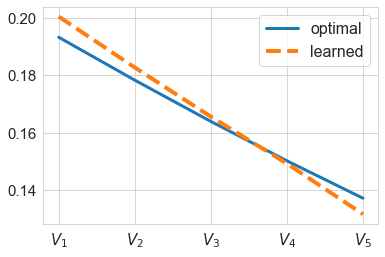
(a) $\{V_{s}\}_{s=0}^{N}$

(b) $\{m_{s}\}_{s=0}^{N}$

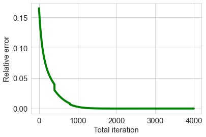
(c) Relative error in total iterations.

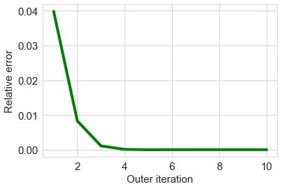
(d) Relative error in outer iterations

Figure 1: Performance of the algorithm when $\lambda_{SE}=1.0$. (True $M=0.75$ and learned $\widehat{M}=0.732$.)

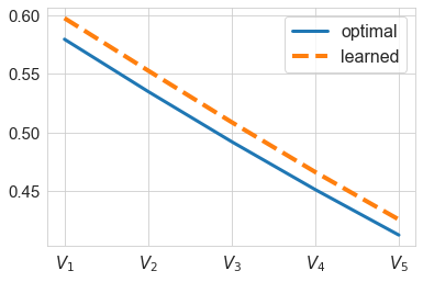
(a) $\{V_{s}\}_{s=0}^{N}$

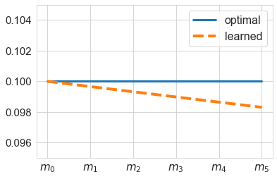
(b) $\{m_{s}\}_{s=0}^{N}$

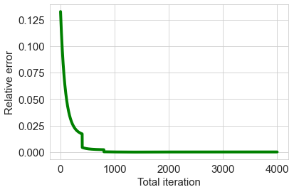
(c) Relative error in total iterations.

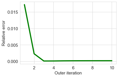
(d) Relative error in outer iterations

Figure 2: Performance of the algorithm when $\lambda_{SE}=3.0$, with true $M=0.75$ and learned $\widehat{M}=0.736$.

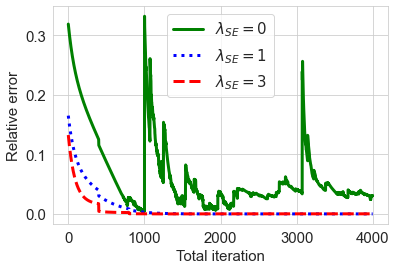
Figure 3: Comparison of relative errors with different $\lambda_{SE}$.

Results.

1. Stability. As seen from Figure 3, when $\lambda_{SE}=0$, i.e., when there is no exploration, the algorithm is unstable. Within each outer iteration, the error level fluctuates when the representative agent updates her policy under a fixed mean field information. At the end of each outer iteration, there is a sudden jump in the error when the population updates its mean field policy. In contrast, the algorithm is stable when exploration is included, i.e., when $\lambda_{SE}>0$.

2. Speed of convergence. As Figures 1(b) and 2(b) show, Shannon entropy ($\lambda_{SE}>0$) improves the speed of convergence to the mean field equilibrium. In fact, the algorithm does not converge without entropy regularization, i.e., when $\lambda_{SE}=0$; On the other hand, the algorithm converges to the equilibrium solution when $\lambda_{SE}=1$ and $\lambda_{SE}=3$. Moreover, the convergence speed is faster with $\lambda_{SE}=3$ than with $\lambda_{SE}=1$, with the former converging to the mean field equilibrium within three outer iterations and the latter in five outer iterations.

3. Accuracy of learned mean field equilibrium. Figures 1(b) and  2(b) show consistency with Theorems 2 and 4. The algorithm is able to learn the mean field information with small errors ($<5\%$) for both cases $\lambda_{SE}=1$ and $\lambda_{SE}=3$.

4. Learning optimal scheduling of the exploration policy. With given parameters, the variance of the Gaussian mean field policy (a.k.a., the optimal exploration scheduling) is a decreasing function of time $t$ for both $\lambda_{SE}=1$ and $\lambda_{SE}=3$. Figures 1(a) and 2(a) suggest that the agent can learn this decreasing function $\{\widehat{\sigma}^{2}_{s}\}_{s=0}^{T}$ with small error $(<5\%)$.

References

- [1] Zafarali Ahmed, Nicolas Le Roux, Mohammad Norouzi, and Dale Schuurmans. Understanding the impact of entropy on policy optimization. In International Conference on Machine Learning, pages 151–160, 2019.
- [2] Berkay Anahtarci, Can Deha Kariksiz, and Naci Saldi. Q-learning in regularized mean-field games. arXiv preprint arXiv:2003.12151, 2020.
- [3] Karl J Aström and Björn Wittenmark. Adaptive control. Courier Corporation, 2013.
- [4] Martino Bardi. Explicit solutions of some linear-quadratic mean field games. Networks & Heterogeneous Media, 7(2):243, 2012.
- [5] Alain Bensoussan, KCJ Sung, Sheung Chi Phillip Yam, and Siu-Pang Yung. Linear-quadratic mean field games. Journal of Optimization Theory and Applications, 169(2):496–529, 2016.
- [6] Jalaj Bhandari and Daniel Russo. Global optimality guarantees for policy gradient methods. arXiv preprint arXiv:1906.01786, 2019.
- [7] Pierre Cardaliaguet, François Delarue, Jean-Michel Lasry, and Pierre-Louis Lions. The Master Equation and the Convergence Problem in Mean Field Games:(AMS-201), volume 201. Princeton University Press, 2019.
- [8] Pierre Cardaliaguet and Saeed Hadikhanloo. Learning in mean field games: the fictitious play. ESAIM: Control, Optimisation and Calculus of Variations, 23(2):569–591, 2017.
- [9] René Carmona, François Delarue, et al. Mean field forward-backward stochastic differential equations. Electronic Communications in Probability, 18, 2013.
- [10] René Carmona, Daniel Lacker, et al. A probabilistic weak formulation of mean field games and applications. Annals of Applied probability, 25(3):1189–1231, 2015.
- [11] René Carmona, Mathieu Laurière, and Zongjun Tan. Linear-quadratic mean-field reinforcement learning: Convergence of policy gradient methods. arXiv preprint arXiv:1910.04295, 2019.
- [12] Sarah Dean, Horia Mania, Nikolai Matni, Benjamin Recht, and Stephen Tu. On the sample complexity of the linear quadratic regulator. Foundations of Computational Mathematics, pages 1–47, 2019.
- [13] Maryam Fazel, Rong Ge, Sham M Kakade, and Mehran Mesbahi. Global convergence of policy gradient methods for the linear quadratic regulator. arXiv preprint arXiv:1801.05039, 2018.
- [14] Zuyue Fu, Zhuoran Yang, Yongxin Chen, and Zhaoran Wang. Actor-critic provably finds Nash equilibria of linear-quadratic mean-field games. arXiv preprint arXiv:1910.07498, 2019.
- [15] Jordi Grau-Moya, Felix Leibfried, and Peter Vrancx. Soft Q-learning with mutual-information regularization. In International Conference on Learning Representations, 2018.
- [16] Xin Guo, Anran Hu, Renyuan Xu, and Junzi Zhang. Learning mean-field games. In Advances in Neural Information Processing Systems, pages 4967–4977, 2019.
- [17] Ben M Hambly, Renyuan Xu, and Huining Yang. Policy gradient methods for the noisy linear quadratic regulator over a finite horizon. Available at SSRN, 2020.
- [18] Ben M Hambly, Renyuan Xu, and Huining Yang. Policy gradient methods find the nash equilibrium in n-player general-sum linear-quadratic games. Available at SSRN 3894471, 2021.
- [19] Elad Hazan, Sham Kakade, Karan Singh, and Abby Van Soest. Provably efficient maximum entropy exploration. In International Conference on Machine Learning, pages 2681–2691, 2019.
- [20] Josef Hofbauer and William H Sandholm. On the global convergence of stochastic fictitious play. Econometrica, 70(6):2265–2294, 2002.
- [21] Zhang-Wei Hong, Shih-Yang Su, Tzu-Yun Shann, Yi-Hsiang Chang, and Chun-Yi Lee. A deep policy inference Q-network for multi-agent systems. In Proceedings of the 17th International Conference on Autonomous Agents and MultiAgent Systems, pages 1388–1396. International Foundation for Autonomous Agents and Multiagent Systems, 2018.
- [22] Rein Houthooft, Xi Chen, Yan Duan, John Schulman, Filip De Turck, and Pieter Abbeel. Vime: Variational information maximizing exploration. In Advances in Neural Information Processing Systems, pages 1109–1117, 2016.
- [23] Minyi Huang, Peter E Caines, and Roland P Malhamé. Large-population cost-coupled lqg problems with nonuniform agents: individual-mass behavior and decentralized -Nash equilibria. IEEE transactions on automatic control, 52(9):1560–1571, 2007.
- [24] Shariq Iqbal and Fei Sha. Actor-attention-critic for multi-agent reinforcement learning. In International Conference on Machine Learning, pages 2961–2970, 2019.
- [25] Daniel Lacker. Mean field games via controlled martingale problems: existence of markovian equilibria. Stochastic Processes and their Applications, 125(7):2856–2894, 2015.
- [26] Daniel Lacker. Mean field games via controlled martingale problems: existence of markovian equilibria. Stochastic Processes and their Applications, 125(7):2856–2894, 2015.
- [27] Daniel Lacker and Thaleia Zariphopoulou. Mean field and n-agent games for optimal investment under relative performance criteria. Mathematical Finance, 2017.
- [28] Jean-Michel Lasry and Pierre-Louis Lions. Mean field games. Japanese journal of mathematics, 2(1):229–260, 2007.
- [29] Timothy P Lillicrap, Jonathan J Hunt, Alexander Pritzel, Nicolas Heess, Tom Erez, Yuval Tassa, David Silver, and Daan Wierstra. Continuous control with deep reinforcement learning. arXiv preprint arXiv:1509.02971, 2015.
- [30] Xiuyuan Lu and Benjamin Van Roy. Information-theoretic confidence bounds for reinforcement learning. In Advances in Neural Information Processing Systems, pages 2461–2470, 2019.
- [31] Horia Mania, Stephen Tu, and Benjamin Recht. Certainty equivalence is efficient for linear quadratic control. In Advances in Neural Information Processing Systems, pages 10154–10164, 2019.
- [32] Gergely Neu, Anders Jonsson, and Vicenç Gómez. A unified view of entropy-regularized markov decision processes. arXiv preprint arXiv:1705.07798, 2017.
- [33] Matthias Plappert, Rein Houthooft, Prafulla Dhariwal, Szymon Sidor, Richard Y Chen, Xi Chen, Tamim Asfour, Pieter Abbeel, and Marcin Andrychowicz. Parameter space noise for exploration. arXiv preprint arXiv:1706.01905, 2017.
- [34] Roberta Raileanu, Emily Denton, Arthur Szlam, and Rob Fergus. Modeling others using oneself in multi-agent reinforcement learning. arXiv preprint arXiv:1802.09640, 2018.
- [35] Daniel Russo and Benjamin Van Roy. An information-theoretic analysis of thompson sampling. The Journal of Machine Learning Research, 17(1):2442–2471, 2016.
- [36] Haoran Wang, Thaleia Zariphopoulou, and Xunyu Zhou. Exploration versus exploitation in reinforcement learning: a stochastic control approach. Journal of Machine Learning Research, To Appear, 2020.
- [37] Haoran Wang and Xun Yu Zhou. Continuous-time mean-variance portfolio selection: A reinforcement learning framework. Available at SSRN 3382932, 2019.
- [38] Weichen Wang, Jiequn Han, Zhuoran Yang, and Zhaoran Wang. Global convergence of policy gradient for linear-quadratic mean-field control/game in continuous time. arXiv preprint arXiv:2008.06845, 2020.
- [39] Michael Wunder, Michael L Littman, and Monica Babes. Classes of multiagent Q-learning dynamics with epsilon-greedy exploration. In Proceedings of the 27th International Conference on Machine Learning (ICML-10), pages 1167–1174. Citeseer, 2010.
- [40] Kaiqing Zhang, Zhuoran Yang, and Tamer Basar. Policy optimization provably converges to Nash equilibria in zero-sum linear quadratic games. In Advances in Neural Information Processing Systems, pages 11602–11614, 2019.