Avoidance, Adjacency, and Association in Distributed Systems Design

Abstract

Patterns of avoidance, adjacency, and association in complex systems design emerge from the system’s underlying logical architecture (functional relationships among components) and physical architecture (component physical properties and spatial location). Understanding the physical–logical architecture interplay that gives rise to patterns of arrangement requires a quantitative approach that bridges both descriptions. Here, we show that statistical physics reveals patterns of avoidance, adjacency, and association across sets of complex, distributed system design solutions. Using an example arrangement problem and tensor network methods, we identify several phenomena in complex systems design, including placement symmetry breaking, propagating correlation, and emergent localization. Our approach generalizes straightforwardly to a broad range of complex systems design settings where it can provide a platform for investigating basic design phenomena.

A fundamental question in the design of complex, multicomponent systems is how the components of the system are arranged.Aikens (1985); Dorneich and Sahinidis (1995); Drira et al. (2007) Arrangement problems, generically, present the challenge of anticipating or identifying “prime real estate”,Owen and Daskin (1998); Shields et al. (2017) i.e. sectors of the system’s architecture that have premium or priority because of the mutual avoidance, adjacency, or association between system components (see Fig. 1). Determining or anticipating components’ patterns of avoidance, adjacency, and association is important in so-called “greenfield” settings, i.e. before design aspects have been specified, and in “brownfield” settings, i.e. when one or more system design aspects have been determined.Dorsey (2003); Adams and Watkins (2008); Hopkins and Jenkins (2008) In both greenfield and brownfield settings, determining the patterns of arrangement and identifying system factors driving those behaviors is crucial for managing, mitigating, or adapting to likely design outcomes.Chalfant (2015)

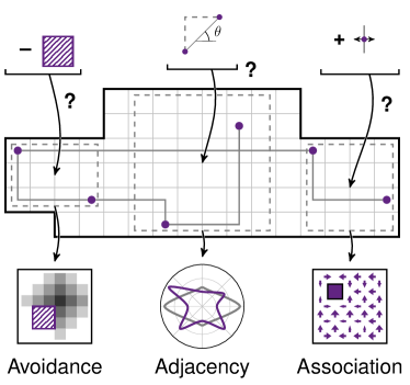
Figure 1: Complex system design raises the question of identifying arrangement patterns of avoidance, adjacency, and association. Avoidance patterns (left) can be probed by testing the “cost” of creating a void in the design. Adjacency patterns (center) describe arrangement motifs found in the design, e.g. angles between the placement of design elements. Association patterns (right) relate to the preference for proximity between design elements, e.g. measures “preferred” locations in adding design elements.

Managing likely design outcomes by identifying patterns of arrangement depends crucially on both a system’s logical architecture, i.e. the set of functional connections between components, and on the system’s physical architecture, i.e. the physical properties of the components and their arrangement in space.Brefort et al. (2018) A system’s logical architecture is essentially topological, and can be treated using network theory techniques.Newman (2010) In contrast, describing the physical architecture of a system is typically done by disciplinary engineering approaches that rest on known physical principles. Treating problems in arrangements that arise from an interplay of a system’s logical and physical architecture requires a framework that bridges a system’s network-theory-level description and its physical/spatial description. Whereas approaches exist at the network theory and at the physical spatial levels, how they can be bridged is an open question.

Here, we show that topological and physical descriptions of complex systems design can be bridged using statistical physics. Using statistical physics we demonstrate a framework that reveals patterns of avoidance, adjacency, and association in arrangement problems. We use an example arrangement problem to concretely demonstrate how our framework can identify patterns of arrangement and how those patterns are driven by the design’s logical and physical architecture, in both greenfield and brownfield settings.

I Systems Physics Framework

I.1 Motivation: Design Challenges Lurk Between Logical and Physical Architectures

Complex systems are typically comprised by several interacting entities. The interactions among the entities are often described at two different levels: the description of what-is-connected-to-what, which is mathematically a graph-theoretic description, and by the description of how the entities physically interact with one another in space, which is described by physics. Taken separately, both levels of description give useful but incomplete insights into design.

The logical architecture’s graph-theoretic description of a complex system design is valuable because it isolates the connections between system elements that underly functionality.Brefort et al. (2018) Functionality in the logical architecture is reduced to the topology of connections, and this connection topology can be analyzed with network theory techniques.Buldyrev et al. (2010); Li et al. (2012); Shields et al. (2016) Network theory approaches to analyzing logical architecture are powerful because they abstract out the system’s physical realization.Newman (2003) However, realizing the logical architecture physically can produce emergent functional connections that are lost when logical architecture is analyzed alone.

The physical architecture describes the realization of a complex system design in terms of physical entities with physical properties. Whereas entities in the logical architecture have abstract interactions that are encoded topologically, in the physical architecture interactions interact mechanically, thermodynamically, electromagnetically, etc., depending on physical factors such as energy consumption and proximity in space. By retaining this level of detail, the physical architecture provides an intimate picture of the performance of design elements. However, this intimate portrait of performance typically describes a single physical architecture instance. What that single instance means for the space of possible designs more generally is often unclear.

Though they can provide key insight into single design instances, both physical and logical architecture descriptions restrict our ability to understand general characteristics of design. This restriction exists because general design characteristics are properties of design problem spaces rather than of design instances. The focus on design instances has been described previously as design organized around “product structures”, i.e., around a particular outcome of the design process.Shields and Singer (2017) Contrasting with product structures are “knowledge structures” that organize the design process around relationships between design elements that persist across instances.Shields (2017)

Searching across instances is key for identifying patterns of avoidance, adjacency, and association that are generic features of design problem spaces. Achieving this requires a different approach. To formulate this approach, the key challenge is in framing knowledge that emerges from collections of possible instances of a system. The problem of many instances that give rise to collective behavior is the underlying principle that motivated the development of statistical mechanics.Gibbs (1902) The fact that an analogous problem emerges in design, i.e. the need to formulate knowledge structures to identify patterns in design space, suggests that statistical physics could serve as the foundation for a similar approach. Fig. 2 illustrates this strategy of attack.

Figure 2: The need to grow from “product structure” approaches, the focus on single design instances, to “knowledge structure” approaches, the patterns of design outcomes or challenges that persist across collections of instances, suggests the applying the framework statistical physics. Statistical physics collectively sums the topological-level description of the logical architecture that expresses the system’s underlying functionality and the physical/spatial description of design instances. Connecting the logical and physical descriptions of design in this way, the resulting “systems physics” picture that emerges bridges between traditional network theory and engineering design approaches.

I.2 Statistical Physics Approach

The need to address the problem of identifying patterns of avoidance, adjacency, and association that persist across spaces of designs points to statistical physics as a framework. To construct this framework there are two key challenges: formulating the design problem as a statistical mechanics model, and extracting from the model the knowledge structures that encode design space properties.

To construct statistical physics models of design, we need two things: the space of states and some metric on this space. For design problems that are studied with optimization techniques like simulated annealing, these two things are already at hand. A generic approach for constructing a statistical physics design framework given a space of possible designs and a set of design objectives was developed in Ref. Klishin et al. (2018a).

Mathematical Formulation—Following Ref. Klishin et al. (2018a), we denote the design space as the set $\{\alpha\}$ consisting of individual design solutions $\alpha$. Each solution $\alpha$ can be quantitatively evaluated with a design objective $\mathcal{O}(\alpha)$. Instead of exclusively focusing on the design that minimizes $\mathcal{O}$, we consider a probability distribution $p_{\alpha}$ over designs.Klishin et al. (2018a) Of all possible normalized probability distributions, we seek one that maximizes the Shannon entropy functional:Jaynes (1957)

$$S[p_{\alpha}]=-\sum\limits_{\alpha}p_{\alpha}\ln p_{\alpha}-\lambda\left(\sum\limits_{\alpha}p_{\alpha}\mathcal{O}(\alpha)-\left<\mathcal{O}\right>\right).$$ (1)

We find the probability distribution by taking a functional derivative $\delta S/\delta p_{\alpha}$ and setting it to zero, resulting in:

$$p_{\alpha}=\frac{1}{\mathcal{Z}}e^{-\lambda\mathcal{O}(\alpha)};\quad\mathcal{Z}=\sum\limits_{\alpha}e^{-\lambda\mathcal{O}(\alpha)},$$ (2)

where $\lambda$ is the design pressure, or the relative importance of the corresponding design objective in driving the distribution. The normalization $\mathcal{Z}$ is known as the partition function and contains a wealth of information on the properties of the whole design space. Mathematically, our study of the design problem is reduced to studying how the distribution $p_{\alpha}$ is affected by soft constraints (design pressure $\lambda$) and hard constraints (the set of available solutions $\alpha$).

Extracting Design Information—With this formulation of design problems as statistical mechanics models, the next challenge is to extract collective properties that encode information about the structure of the design problem and the space it lives in. Doing this typically requires computing sums over a combinatorially large set of $\alpha$, which relies on various problem-specific mathematical techniques. For simple scenarios involving only one or two nodes with integrable interactions, prior work has shown that this can be done by coarse-graining to extract effective, so-called Landau, free energies.Klishin et al. (2018b) We expect that effective free energy approaches will, as they do in the ordinary statistical mechanics of particles, provide the means to gain insight into the collective properties of more complex design spaces. However for more complex design spaces, again as is the case in the ordinary statistical mechanics of particles, some mathematical techniques are required to study systems that lack closed-form, integrable interactions.

To meet the challenge of extracting information about design spaces with complex forms of interaction it is useful to take cues from the structure of the problem. For complex problems the advantage of the logical architecture is that it reduces the complexity of interactions among elements to simple, binary, yes/no connections. The disadvantage of this simplicity is that it loses the richness and specificity of the underlying design problem. This suggests a more complete treatment of the design problem would be to “decorate” the topological description of the logical architecture with information about the “topography” of the underlying design space and its physical architecture. This topographic decoration can be carried out by encoding the design space as a tensor network.

Tensor Network Formulation—Tensor networks were originally introduced as a graphic notation for geometric tensors,Penrose (1971) but over the last 25 years have grown into powerful computational tools for storing and manipulating high-rank data. The tensor network computations are especially efficient when the connections are sparse. This property spurred the popularity of tensor networks in a broad range of applications, from encoding entangled wavefunctions in quantum condensed matter systems,Verstraete et al. (2008); Schollwöck (2011); Orús (2014) to performing precision quantum chemistry calculations,Chan and Sharma (2011) renormalizing lattice models,Xie et al. (2009); Levin and Nave (2007) solving constraint counting problems,Biamonte et al. (2015); Kourtis et al. (2019) accelerating numerical linear algebra,Cichocki et al. (2016, 2017); Oseledets (2011) and learning multilinear classifiers in machine learning.Stoudenmire and Schwab (2016) Across these applications, tensor networks serve as an information structure that contains an exhaustive but raw description of the system.

We use tensor networks to bridge the logical and physical descriptions of a design problem space. Network nodes encode the design elements’ topography in the physical space of their placement and their properties. Network connections encode the functional connection topology and topography of the physical interaction of design elements based on their spatial location and physical properties. The topography–topology connection that the tensor network encodes has the useful side benefits that it provides a simple graphical representation of the interaction of design elements, and that well-developed methods exist for extracting information from tensor networks.

Tensor networks encode information about the design space, but knowledge about patterns of avoidance, adjacency, and association among design elements, has to be extracted with special techniques. Extracting this information requires adding specifically formulated pieces to it that represent key design questions (or, in physics language, observables or order parameters). We formulate design questions about avoidance, adjacency, and association among design elements by acting on the tensor network with a combination of elementary “moves”. The moves yield patterns of the placement over sets of solutions in design space, that are computed via contraction of tensor networks. See Appendix A for a detailed description of moves and contraction.

We note that recasting the problem in the language of tensor networks is an exact operation. The tensor networks shown on figures below are not qualitative illustrations, but mathematical formulas written in a graphical language explained in detail in Appendix A. Though there are many ways to perform and illustrate statistical mechanics computations for systems of simple topology (e.g. well-mixed, lattice, tree), to our knowledge tensor networks are the first method that can deal with arbitrary complex topology. Alternatively, we could evaluate the arrangement patterns by averaging over a representative sample of solutions with Monte Carlo methods, however that would engender statistical and sampling issues that could restrict interpretability. Tensor network computations are free of those issues, at least for the present problem. The numerical contraction computations introduce a controlled approximation error via SVD truncation, but it is of qualitatively different kind than finite sample error.

I.3 Example Model System

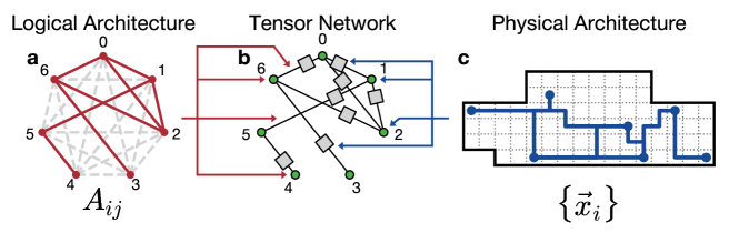
Figure 3: Tensor network bridges the logical and physical descriptions of the design space for an example Naval Engineering arrangement problem. (a) The logical architecture is represented graphically by a network of seven functional units (red circles) and their specific pattern of functional connections (red lines), and algebraically with the adjacency matrix $A_{ij}$. The dashed gray lines represent the non-links in the network, which do not directly drive the arrangement but can be investigated. (b) The structure of the whole design space is contained in an information structure in form of a tensor network. Logical architecture determines the network pattern in which the tensors are connected, while physical architecture determines the contents of both site and coupling tensors. (c) The physical architecture is represented graphically by a square grid within a complex hull shape, and algebraically by the set of possible unit locations $\{\vec{x}_{i}\}$. A particular arrangement consists of the placement of all seven functional units within the hull and the routing of all functional connections between them (blue circles and lines).

Functional Units and Connections—To demonstrate the Systems Physics analysis and tensor network computations on a concrete example of a design problem, we first define the specific logical and physical architectures for the problem. We use a problem from Naval Engineering,Shields et al. (2017) in which the functional units of a shipboard system need to be arranged within the hull of a naval vessel, while respecting their functional connections, such as pipes or cables. The network pattern of connections constitutes the logical architecture, also represented algebraically as an adjacency matrix $A_{ij}$. We find a wide variety of network motifs arise in networks of as few as $n=7$ functional units without any graph symmetries (Fig. 3a), which we will study in the remainder of this work.

Ship Hull—We position units and connections within a ship hull that we represent, following Shields et al. (2017), by a 2D square grid with a complex, but fixed boundary (Fig. 3c). We constrain all connections within the ship hull to always run along a shortest path between the two functional units; we choose our hull to be $L_{1}$-convex to ensure that at least one shortest path exists between any pair of cells. We find that hull models with a few tens of cells are sufficient to establish placement patterns; computations reported below are for hulls with $Y_{0}=78$ distinct cells for unit placement each labelled as $\vec{x}_{i}$.

Design Objectives—Picking the locations of all units and the routings of functional connections between them defines a design solution $\alpha=(\{\vec{x}_{i}\},\textsf{routing})$. In early-stage design, design architectures are typically not fixed, therefore the full combinatorial design space needs to be considered. Each design solution is quantitatively evaluated with a design objective $\mathcal{O}(\alpha)$, here we model routing cost:

$$\lambda\mathcal{O}(\alpha)=\lambda\sum\limits_{ij}A_{ij}CL_{1}(\vec{x}_{i},\vec{x}_{j})\;,$$ (3)

where $L_{1}$ is the “Manhattan” distance between the two cells, $C$ is the cost per unit distance, and $\lambda$ is the design pressure. Given the placement of units, we consider all allowed shortest paths between them. By definition, all shortest paths have the same length, so the value of $\mathcal{O}$ doesn’t depend on the particular routing chosen, yet the number of routings is important. To account for the redundancy of routings, we introduce an effective design objective:

$$\lambda\mathcal{O}_{\textsf{eff}}(\{\vec{x}_{i}\})= \sum\limits_{ij}A_{ij}f(\vec{x}_{i},\vec{x}_{j};T)\;;$$ (4)

$$f(\vec{x}_{i},\vec{x}_{j};T)= \frac{C}{T}L_{1}(\vec{x}_{i},\vec{x}_{j})-\ln n_{\textsf{rout}}(\vec{x}_{i},\vec{x}_{j})\;,$$ (5)

where $n_{\textsf{rout}}$ is the number of shortest routings between $\vec{x}_{i}$ and $\vec{x}_{j}$ within the ship hull, typically growing with distance. The routing lengths $L_{1}(\vec{x}_{i},\vec{x}_{j})$ and the number routings $n_{\textsf{rout}}(\vec{x}_{i},\vec{x}_{j})$ are fully determined by the shape of the hull and can be precomputed, stored as matrices, and scaled by the design pressure as needed.

Tensor Network—The representation of the design space in form of a tensor network depends on both logical and physical architectures (Fig. 3b). Logical architecture in form of the network $A_{ij}$ determines the pattern in which the site and coupling tensors are connected. Physical architecture determines the set of available locations for all units $\{\vec{x}_{i}\}$ that is used as index for all tensors. The effective design objective $f(\vec{x}_{i},\vec{x}_{j};T)$ determines the entries of the coupling tensor. See Appendix A for a detailed mathematical discussion.

Greenfield/Brownfield Settings—In the above formulation, the design space $\{\alpha\}$ of the problem is the space of all possible arrangements of each functional unit $\{\vec{x}_{i}\}$, and is it necessary to establish a means of distinguishing units with fixed and variable position. This distinction is necessary because the formulation needs to address arrangement before or after some of the units have been placed. We refer to situations in which no units have fixed placement as greenfield settings. Greenfield settings are generically associated with green color-coding in results figures that follow. Also, we refer to situations in which one or more units have fixed locations as brownfield settings. Brownfield settings are generically associated with brown color-coding in results figures that follow. In Results figures that describe brownfield settings that combine placed units with yet-to-be-placed units we make a visual distinction between the two by color-coding placed units and their effects brown and yet-to-be-placed units green.

Low Cost, High Flexibility, and Crossover Regimes—The formulation of design problems in terms of spaces of solutions weighted by objectives of the form of Eq. (5) has been studied in Ref. Klishin et al. (2018a). As in Ref. Klishin et al. (2018a) we expect that the choice of the design pressure associated with each objective (general case: Eq. (2); this model: Eq. (3)) will have qualitatively distinct effects on design outcomes.Klishin et al. (2018a) To maximize generality, we study design pressures that correspond to multiple behavioral regimes. We do this by first expressing the design pressure via its inverse $\lambda=1/T$, where $T$ is the cost tolerance. Low cost tolerance means that minimizing the routing cost $\mathcal{O}$ is a strong driver of a design solution choice, whereas high cost tolerance means that the choice among the design solution is not driven by cost. Ref. Klishin et al. (2018a) showed that the system driven by this design objective undergoes a large-scale rearrangement (akin to a phase transition, but at finite-size) around $T_{\textsf{crit}}=C/\ln 2\approx 1.44C$. We pick $C=1$ to fix the measurement units for $T$. $T<T_{\textsf{crit}}$ favors low cost and we therefore expect units to organize into motifs that facilitate short (cheap) connecting paths. We expect this setting to be characterized by effective attraction. $T>T_{\textsf{crit}}$ favors maximal flexibility and we expect units to organize into motifs that facilitate maximizing routing degeneracy. We expect this setting to be characterized by effective repulsion. We expect that for $T\approx T_{\textsf{crit}}$ where cost and flexibility drivers are competing on near-equal footing there will be a crossover in behavior.

II Results

Having formulated our statistical mechanics approach and introduced the model system, we turn to the arrangement patterns of distributed design elements depicted in Fig. 1 and the quantitative drivers of the patterns of avoidance, adjacency, and association. We find that all three patterns manifest behaviours that are analogous to behaviours observed in condensed matter physics.

The avoidance patterns we operationalize here describe the propensity for functional units in design to preferentially avoid certain regions of space. In our example system, we test this by introducing a void within the ship hull and determining the effect of the void placement on the design objectives.

The adjacency patterns we operationalize here describe the propensity for design elements to arrange into characteristic relative arrangements, or motifs, that persist despite the absolute placement of the elements. In our example system, we compute the distribution of pairwise relative directions between the units and study the effects of topological distance and topology change.

The association patterns we operationalize here describe the propensity for an element introduced into a design to locate preferentially relative to the placement of already-existing functional units. In our example system, we compute the how placement affects design objectives, and find effective forces that drive individual units to preferred locations in a later stage of design.

Our results for each of these three arrangement patterns are described below.

II.1 Avoidance

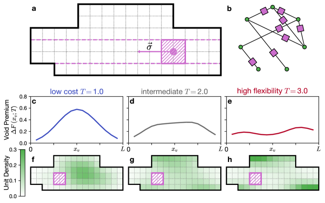
Figure 4: Void premium quantifies the cost of avoidance of reserved space across the whole design space in a greenfield scenario. (a) Schematic of the ship hull and square cells within (Physical Architecture). Pink square represents a void where unit placement is prohibited, driven by the void design stress $\vec{\sigma}$ along the center line of the hull (pink dashed lines). (b) Tensor network used to compute the void premium, with each coupling tensor modified. (c-e) Graphs of void premium (void free energy $\Delta F(x_{v};T)$) against the void coordinate $x_{v}$ for three values of $T$ (color coded). (f-g) Functional unit density in presence of the void.

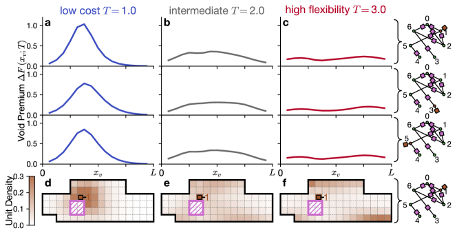
Figure 5: A brownfield scenario, such as anchoring one functional unit, sharpens the void premium curve. (a-c) Graphs of void premium (void free energy $\Delta F(x_{v};T)$) against the void coordinate $x_{v}$ for three values of $T$ (columns, color coded) and different choice of the anchored unit (rows, anchor shown in the tensor network on the right). (d-e) Functional unit density in presence of the void and unit 1 anchored in the indicated cell (brown square).

Void Premium—The interplay of logical and physical constraints among design elements induces a complex landscape for element placement. Intervening in that landscape by reserving space for future use could induce functional units to make a complex, collective rearrangement to avoid the reserved space. We characterize the cost of avoidance by computing the void premium that must be paid to forbid any units to be placed in the reserved space.

We implement reserved space mathematically by creating a void $2\times 2$ cells in size. In the results below we introduce the void on the hull midline, though in general it could be placed anywhere. We vary the horizontal location of the void, $x_{v}$, from zero to the hull length $L$ (see Fig. 4a). We compute the cost of the void via the tensor network approach by suppressing several rows and columns of the coupling tensor (see Appendix A). Contracting the modified tensor network results in a modified partition function, which is smaller or equal to the original one $\mathcal{Z}(x_{v};T)\leq\mathcal{Z}(T)$. The ratio of the two partition functions defines the non-negative free energy:

$$\Delta F(x_{v};T)=-\ln\frac{\mathcal{Z}(x_{v};T)}{\mathcal{Z}(T)}.$$ (6)

We take this void free energy as a measure of the void premium, the effective “cost” of the avoidance of a specified region in space.

Void Design Stress—The magnitude of the void premium $\Delta F$ corresponds to the placement opportunity cost for the functional units. To understand this opportunity cost, note that functional units that are not yet placed form a greenfield “cloud” of possibilities within the hull, the location and density of which depends on the cost tolerance $T$. Cutting a void from a dense part of the cloud costs a lot of free energy, whereas cutting a cloud from a sparse part of the cloud costs almost nothing. In this way, scanning the void free energy along the void coordinate $x_{v}$ gives a direct probe of the morphology of the cloud. Conversely, if we regard the unit positions as fixed, and the void as moveable, the cloud of units drives the void with an effective force $\sigma=-\Delta F/\Delta x_{v}$, which we call void design stress. The void free energy and design stress are then a concise description of the collective effect of avoidance in functional unit placement.

The void premium and void design stress give a description of collective avoidance effects in placement. These effects can be examined in greenfield and brownfield settings.

Greenfield—We studied avoidance metrics in greenfield settings, i.e. before any unit data have been fixed, in three design regimes specified by cost tolerance $T$. We plot results in Fig. 4c-e. At subcritical $T=1.0$ (low cost priority), the void free energy curve shows a clear single maximum in the middle of the hull, and two minima on the ends of the hull. At near-critical $T=2.0$ (cost-flexibility tradeoff) the curve maintains the same qualitative shape, but the maximum gets flatter. At supercritical $T=3.0$ (high flexibility priority), the curve shape flips to have a local minimum at the center of the hull, surrounded by local maxima on two sides. In other words, at low $T$ the void prefers to be at either of the two ends of the ship (but a choice needs to be made in favor of one of them). In contrast, at high $T$ the void prefers to be in the center of the ship. Thus the change from designing for flexibility (high $T$) to designing for cost (low $T$) induces a change from one architecture class (central-void) to two architecture classes (bow-void and stern-void). This collective effect is analogous to symmetry-breaking phase transitions in conventional physical systems.Goldenfeld (1992)

To understand the origin of the symmetry breaking we note that void free energy is a proxy for the morphology of the unit cloud. To illustrate the shape of the cloud in a different way, we approximate the cloud density as a sum of one-unit densities $\rho(\vec{x})=\sum_{i}p_{i}(\vec{x})$ and plot densities as heatmaps in Fig. 5f-h. These heatmaps are approximate because, unlike the void free energy curves, they ignore the correlations in unit placement. At low $T$ (panel f), units attract each other and thus preferentially form a cloud in the center of the hull and push the void to either side of the hull. At near-critical $T$ (panel g), the distribution becomes more homogeneous throughout the hull, flattening the curve. At high $T$ (panel h), functional units strongly repel one another, concentrating near the edges of the hull. This leaves the center nearly empty, resulting in a single void free energy minimum.

Brownfield—Both the void free energy curve and the unit cloud morphology can, however, change dramatically in brownfield settings, e.g. if even one unit is fixed to a specific location in space. We pick the location indicated with the brown square in Fig. 5d-f and fix one unit there. We choose three different units to fix: unit 3 (which has 1 functional connection), unit 5 (2 functional connections) and unit 1 (3 functional connections). We plot the resulting void free energy curves in panels a-c, and unit clouds in panels d-f.

Consider first the low-cost regime $T=1.0$ (Fig. 5a,d). In the greenfield setting (Fig. 4f) units positions were determined solely by ship geometry, and formed a dense cloud in the middle of the ship (Fig. 4f). Fixing a unit position places an additional constraint on unit positions, and forces the unit cloud to condense around it (Fig. 5d). Because of this condensation, the void free energy curve becomes simultaneously steeper and more focused around the fixed unit point (panel a), but decays faster close to the edges of the hull. The void free energy cost also depends on the topological position of the anchored unit: it is highest for the most-connected unit 1 (bottom curve) and lowest for the least-connected unit 3 (top curve).

At the near-critical and supercritical $T=2.0,3.0$ the anchored unit similarly creates a reference point for the cloud, but the units in the cloud repel from that point. When repulsion and attraction are nearly balanced at $T=2.0$, the cloud profile becomes nearly uniform and is not strongly affected by the fixed unit (compare Fig. 4g and Fig. 5e). Similarly, fixing a unit at supercritical $T=3.0$ creates a point of strong repulsion, forcing the unit cloud to the opposite corners of the ship hull (Fig. 4h and Fig. 5f). At both values of $T=2.0,3.0$, the cloud morphology is not affected strongly by the single fixed unit position, and thus the brownfield void premiums (Fig. 5b-c) closely resemble their greenfield couterparts (Fig. 4b-c). Discussion of the effects of avoidance on unit positions, i.e. backreactions on the cloud, can be found in Appendix B.

Avoidance: Logical–Physical Architecture Interplay—The above avoidance analysis gives a case study of basic phenomenology of the interplay between design pressure (favoring low-cost vs high-flexibility) and the logical and physical architecture. Shifting the design priority from low-cost to high-flexibility changed the interaction between pairs of functional units. However, unit interactions were modulated by connection topology (i.e., logical architecture) and by the spatial domain (i.e., the physical architecture). We captured the effect of these complex interactions on spatial avoidance the unit clouds in Figs. 4,5. However, within the unit clouds, the interplay of design pressure with the logical and physical architectures also induces emergent coupling. This emergent coupling within the cloud induces patterns of adjacency and association between units, which we turn to next.

II.2 Adjacency

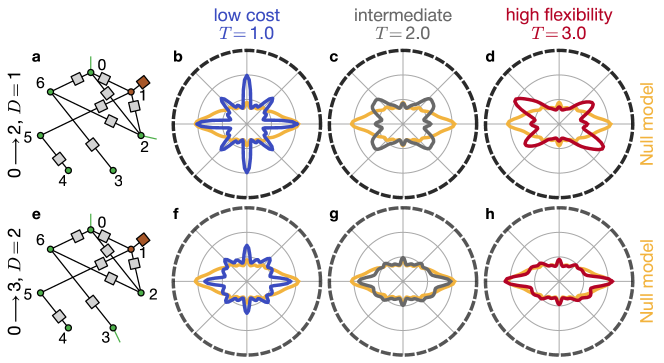
Figure 6: Bond diagrams quantify the adjacency patterns for both directly and indirectly connected functional units. (a-b) Tensor networks used for computations of bond diagrams for two pairs of units, one connected directly (0$\to$2, $D=1$), the other indirectly (0$\to$3, $D=2$). The site tensors in the measured pair have external legs (green). The unit 1 is anchored in the center of the hull (brown square). (c-h) Bond diagrams for the angle between the two units of the pair, for two different pairs (rows) and three values of $T$ (columns, color coded). Yellow curve shows the null model of the bond diagram, identical for all graphs. Black rim of bond diagram axes indicated the topological distance $D=1$, gray rim indicates $D=2$.

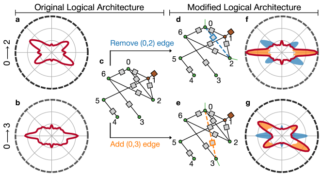
Figure 7: Small changes of Logical Architecture lead to large changes of adjacency patterns, visible in the difference of bond diagrams. Panels a-c correspond to the original Logical Architecture, while panels d-g illustrate two different changes of Logical Architecture. (a-b) Bond diagrams at $T=3.0$ for two pairs of units, 0$\to$2 ($D=1$) and 0$\to$3 ($D=2$). (c) Tensor network used for computations of bond diagrams with original Logical Architecture, external legs not shown. (d) Tensor network used for computation of the 0$\to$2 bond diagram when the functional connection (0,2) is removed (blue dashed line). (e) Tensor network used for computation of the 0$\to$3 bond diagram when the functional connection (0,3) is added (orange dashed line). (f-g) Resulting bond diagrams (dark red curve) with highlighted positive difference (orange shading) and negative difference (blue shading) with respect to the bond diagrams at the original Logical Architecture (panels a-b). Black rim of bond diagram axes indicated the topological distance $D=1$, gray rim indicates $D=2$.

Whereas our avoidance analysis derives from and illustrates the basic morphology of the unit cloud within the ship hull, questions about unit adjacency derive from correlations within the cloud, and the emergent coupling between units that arise.

Bond-Diagram Measures of Adjacency—To determine how emergent coupling between units leads to arrangment motifs, we consider pairs of units and their relative positions. We examine pairs of units in 2D space, and express motifs as the polar angles $\theta(i\to j)$, which vary along with the positions of the units in the cloud. Across the cloud, the angle takes form of a probability distribution $p_{i\to j}(\theta)$. This distribution is analogous to the bond order that is used to describe structure in condensed matter.Steinhardt et al. (1983); Roth and Denton (2000) In condensed matter, bond angles are whole-system aggregate measures of adjacency. Here, the heterogeneous connectivity of design elements yields “bond” diagrams that are specific to each pair of units $i,j$. Depending on whether the units $i$ and $j$ are directly connected or not ($A_{ij}=1\;\text{or}\;0$), the bond diagrams illuminate the strength of direct or emergent adjacency patterns.

Computational Approach—To compute the bond diagrams mathematically, we use tensor networks to compute the raw 2-unit marginal distributions $p(\vec{x}_{i},\vec{x}_{j})$ (Fig. 6a,e), and convert them into the angular distributions $p_{i\to j}(\theta)$ using Kernel Density Estimation to reduce the numerical artifacts (see Appendix A). In order to demonstrate more sharply defined bond diagrams, we assume that one unit has already been placed (anchored) in the center of the hull and all other units need to be placed with respect to it. The bond diagram $p_{i\to j}(\theta)$ of any pair of units is not uniform with respect to the angle $\theta$ even if the units are not connected at all, directly or indirectly. This non-uniformity is driven by the shape of the hull, a manifestation of the physical architecture, and we account for it by computing null model $p_{0}(\theta)$ of the bond diagram (see Appendix A). Differences between the null model and computed bond diagrams are indicators of interaction-driven adjacency. This interaction driven adjacency depends on unit connectivity; we use a topological distance, $D(i,j)$ metric. $D(i,j)$ is the minimal number of network hops to get from unit $i$ to unit $j$. In our example problem, the minimal number of hops varies from 1 (e.g. units 0$\to$1) to 5 (e.g. units 3$\to$4).

Direct Adjacency—We show topological distance, bond diagrams, and the null model for our model in Fig. 6 in form of polar plots for two example unit pairs (corresponding plots for all unit pairs are given in Appendix B). We start discussion with the bond diagrams for direct adjacency (0$\to$2, $D=1$). At subcritical $T=1.0$ (panel b) most units are located very close to each other, either in cardinal or intercardinal directions (orthogonally or diagonally), resulting in a bond diagram with a strong eightfold signal. At near-critical $T=2.0$ (panel c) the orthogonal attraction is balanced with diagonal repulsion, resulting in a bond diagram with smaller peaks. At supercritical $T=3.0$ (panel d) the units are located relatively far from each other and prefer diagonal relative location (since diagonal location allows them to maximize their routing entropy), resulting in a fourfold, X-shaped signal. The symmetry of the fourfold signal is further broken by anchoring the unit 1. This additional symmetry breaking is driven by the high density of units in top-left and bottom-right corners of the hull (see Fig. 4).

Emergent Adjacency—Across the whole $T$ range, the bond diagrams for direct adjacency are significantly different from the null model. However, adjacency can also be induced for indirectly connected unit pairs. The indirectly connected unit pair 0$\to$3 shows emergent adjacency, since its bond diagram is different from both the direct adjacency and the null model (Fig. 6f-h). The bond diagrams for unit pairs with even larger topological distance the bond diagrams gradually approach the null model (see Appendix B), following the intuition of decay of correlation functions with distance in condensed matter systems. This observation suggests the general takeaway: at large topological distance bond diagrams always approach the null model, and thus are fully determined by the Physical Architecture; at small topological distance the bond diagrams depend strongly on both the design pressure $T$ and the explicit details of Logical Architecture. However, our results reveal that for emergent adjacency topological distance is a good predictor of strength but is not a good predictor of shape.

Logical Architecture Modifications—To further test the interplay between Logical Archiecture and Adjacency, we investigate what happens to bond diagrams when we modify the Logical Architecture. We consider two types of modifications: removing an existing functional connection (Fig. 7d), or adding a new one between two units (Fig. 7e). Instead of comparing the resulting bond diagrams to the null model again, we focus on the difference between bond diagrams before and after modification (panels f-g). Addition: The effect of adding the (0,3) connection is strong. We can anticipate that with the added direct adjacency, the adjacency pattern should approach that of other directly adjacent units. The fourfold signal that results (panel g) is a signal of this. Since neither of the units 0 or 3 is explicitly anchored in space, at high $T=3.0$ they want to be positioned at the opposite ends of the longest diagonal available within the hull, in this case the diagonal from top-left to bottom-right corners, similarly to the original adjacency 0$\to$3 (Fig. 6d). Removal: Like for addition the effect of removing the (0,2) connection is dramatic, however the result is unexpected. Instead of fourfold diagonal direct adjacency, the two units now have twofold horizontal emergent adjacency (panel f). The reason for this is that with the (0,2) connection removed, the units 1-2-6-0 now form a rhombus. Unit 1 is fixed in space, and because of high $T=3.0$ all unit pairs prefer to have diagonal adjacency. In this case the units 0 and 2 on the opposite corners of the rhombus will have an orthogonal adjacency, of which only horizontal adjacency manifests because the ship hull is larger in length than height.

Adjacency: Changes and Constraints Drive Patterns—We showed that the irregular, complex-network nature of a system’s Logical Architecture drives the patterns of direct and emergent adjacency. We showed adjacency patterns can change significantly with changes in Logical Architecture. One outcome of this approach was the ability to detect emergent adjacency. The emergent effects we observed were with a single fixed unit. Though having having few fixed units is a characteristic of early-stage design, later-stage design situations will result in more fixed units. Fixing more units will induce more constraints, and further constraints will complicate the interplay of the logical and physical architecture. A more complicated logical–physical architecture interplay should induce more complex patterns of association between units, which we will examine next.

II.3 Association

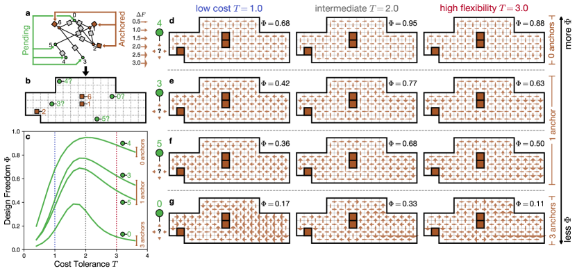
Figure 8: Early stage design decisions determine the association patterns and design freedom for subsequent ones. (a) Tensor network used for association computations. Three out of seven units have already been anchored to specific locations (brown), other four are pending placement (green). External legs not shown. (b) The units 1,2,6 are anchored at the indicated locations within the ship hull (brown squares). The units 0,3,4,5 can still be placed in many locations, some demonstrated for an example (green circles). (c) Graph of the design freedom $\Phi$ for the four units without anchors across a range of cost tolerance $T$. Brown brackets on the right indicate that units with more adjacent anchors have less remaining design freedom. Vertical dotted lines indicate the $T$ values investigated in more detail in panels (d-g), as well as in avoidance and adjacency patterns. (d-g) Design stress $\Delta F$ patterns for the placement of each pending unit (rows in order of decreasing design freedom $\Phi$) at three values of $T$ (columns, color coded). Legend for design stress magnitude $\Delta F$ is shown to the left of panel (d).

Analyzing association patterns extends our avoidance and adjacency investigations to situations in which multiple, pre-existing constraints restrict functional units, i.e. in brownfield settings. These settings model either of two situations: (i) actual late-stage design in which multiple functional units have been fixed during preceding design stages, or (ii) an early-stage design investigation of hypothetical late-stage situations under different decision scenarios.

Constraints and Localization—In either case, the expectation that multiple active constraints will drive complex forms of interaction suggests that identifying patterns of association that result will require different techniques than identifying patterns of avoidance and adjacency. In general we expect that patterns of association arising from multiple constraints will localize those patterns relative to fixed design elements. This suggests that metrics of association patterns should signal a tendency toward (or away from) placement proximity relative to fixed elements, either globally or locally. Here, for a global signal we adapt measures of emergent localization to compute a scalar design freedom for unit locations. For a local signal we compute the design stress associated with specified, hypothetical unit placement.

To study the effect of added constraints, their interplay with the logical and physical architecture and the resulting localization, we employ the same model system as in the avoidance and adjacency investigations. However we introduce constraints that fix units 1,2, and 6 to specific locations. We investigate the emergent localization of the other 4 units with two metrics via the global design freedom $\Phi$ and local design stress $\Delta F$. Results are shown in Fig. 8 and broken down below.

Global Signal of Association: Design Freedom Mathematically, both global and local metrics of localization use a tensor network computation of the marginal probability distribution $p(\vec{x}_{i})$. The conversion of the distribution into design freedom is inspired by the metric of existence area, commonly used in studies of the Anderson localization of wavefunctions in disordered media and the localization of vibrational eigenmodes.Thouless (1974); Filoche and Mayboroda (2009) We define design freedom as:

$$\Phi=\frac{1}{Y_{0}}\frac{\left(\sum\limits_{\vec{x}}p(\vec{x})\right)^{2}}{\sum\limits_{\vec{x}}p(\vec{x})^{2}}\;,$$ (7)

where the normalization $Y_{0}$ is the total number of cells within Physical Architecture; in this example $Y_{0}=78$. Given this normalization, $\Phi$ takes a value between 0 and 1 and has the meaning the effective fraction of the total area available for unit placement, if the distribution was uniform. For a unit with uniform distribution $p(\vec{x}_{i})=const$, $\Phi$ would be 1, whereas for an anchored unit $\Phi$ would be $1/Y_{0}\to 0$.

Because of the heterogeneous connectivity of the logical architecture, design freedom $\Phi$ varies between units. The variation between units is in addition to variation with design pressure, via changing cost tolerance $T$. Fig. 8c plots $\Phi(T)$ by unit, and shows that all units have design freedom peaks near $T\approx 2.0$. In the range of this near-critical $T$, cost (effective attraction) and flexibility (effective repulsion) drivers of unit interactions balance and allow the units to explore the largest range of placement. As well, we observe $\Phi(T)$ to fall into three groups according to how constrained each unit is. Unit 4 is not directly connected to any of the anchored units and thus enjoys the largest design freedom, almost approaching $\Phi=1$. Units 3 and 5 are each connected to one anchored unit and thus have intermediate $\Phi$. Unit 0 is connected to all three anchored units and thus has the lowest $\Phi$ which quickly decays at both low and high $T$.

Local Signal of Association: Design Stress—Whereas $\Phi$ serves as an global scalar metric of design freedom, it is also important to understand how global design freedom is distributed locally. This local distribution is captured by design stress. Design stress is closely related to an effective (Landau) free energy (LFE), defined as follows:

$$F(\vec{x}_{i})=-\ln p(\vec{x}_{i})+C\;,$$ (8)

where $C$ is an arbitrary additive constant. We chose a convention where $C$ is such that the minimal value of $F$ is zero. The LFE can be interpreted as an effective design objective for the chosen degree of freedom, given that other degrees of freedom have been fixed or integrated out. This interpretation is analogous to the void premium (Eq. 6) in our avoidance investigation, but instead of the effects of unit placement on voids, here we examine the effects of unit placements on one another. Similar to the definition of void design stress via a spatial difference, the difference of LFE between two horizontally or vertically adjacent cells is the design stress $\Delta F$. Design stress is then an effective “force” that pushes individual functional units towards their preferred locations.Klishin et al. (2018a, b) Compared with global design freedom, design stress patterns give a more detailed picture of effective localization.

Fig. 8d-g presents the design stress patterns for all four pending units at three values of $T$. Design stress is represented by brown arrows drawn across the boundary of two adjacent cells and pointing from higher to lower LFE. In other words, to decrease LFE and reach lower values of its effective design objective, a unit needs to follow the arrows towards a basin. As the basin gets smaller and its walls get steeper, the pending units become more closely associated with the anchored ones and thus exhibit stronger emergent localization. The localization effect is strongest at lowest $T$, where all of pending units are strongly attracted to the two anchored units 1,6 in a single basin. The basin is steepest for the most constrained unit 0, less steep for the units 3,5, and the shallowest for the least constrained unit 4, consistent with our expectation based on design freedom $\Phi$. At higher $T=2.0,\,3.0$, the constrained unit 0 develops complex LFE and design stress landscapes with multiple local minima, maxima, and ridges (panel g). Units 3,5, connected respectively to the anchored units 6 and 1 in the center of the hull, show an X-shaped pattern of LFE (panels e,f), similar to the bond diagrams for directly connected unit pairs, e.g. Fig. 6d. Lastly, the unit 4 is not connected to any of the anchored units, instead it is “dangling off” unit 5 and thus shows almost nonexistent design stress across the whole hull (panel d).

Association: Interaction and Decision Drivers—Both the design stress and design freedom metrics show that the association patterns and the emergent localization phenomenon strongly depend on the position of both the fixed and the pending units within the logical architecture. The logical architecture alone gives an interpretation of the emergent localization result by counting the anchored neighbors. However, fully predicting localization requires examining the logical–physical architecture interplay that arises from the systems physics analysis. Unlike the simplified unidirectional design stress discussed in Ref. Klishin et al. (2018b), in this system the design stress pattern is emergent both from unit interactions and from previous design decisions. Chaining design decisions into sequences and achieving optimal control of emergent localization stands out as an important question for further study.

III Discussion

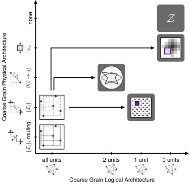
Figure 9: System exploration across levels of detail in physical and logical architectures via two orthogonal directions of coarse-graining. Horizontal axis represents the reduction in the number of functional units explicitly considered. Vertical axis represents the reduction in spatial detail considered. Black arrows represent the computational pathway across the study of avoidance, adjacency, and association patterns. The full design objective $\mathcal{O}$ (Eqn. 3) depends on all unit locations and routings. The effective design objective $\mathcal{O}_{\textsf{eff}}$ (Eqn. 5) depends only on locations of all units. The association pattern considers detailed location $\vec{x}_{i}$, but only for a single unit. The adjacency pattern reduces the spatial detail to just the relative direction $\theta(i\to j)$ between two units. The avoidance pattern further reduces the spatial detail to just the void position $x_{v}$ as a single collective coordinate of the unit cloud. Finally, the partition function $\mathcal{Z}$ loses all detail of physical and logical architecture and summarizes the properties of the whole design space.

In this paper we showed that questions of avoidance, adjacency, and association among the elements of complex, distributed systems hinge on the interaction between logical- and physical-architecture description planes. We bridged these descriptive planes with statistical physics techniques and showed that patterns of avoidance, adjacency, and association can be mapped for an example system.

Design Phenomena: Symmetry-Breaking, Emergent Adjacency, Localization— Our mapping of avoidance gave a space premium landscape. We found this landscape to undergoe a symmetry-breaking transition with a change from design pressure that prioritizes high flexibility to pressure that prioritizes low cost (Figs. 4,5). Our mapping of adjacency gave a description analogous to “bond” directions in matter systems. From this bonding description we observed that indirectly connected design elements developed emergent adjacency (Fig. 6). We also found large downstream changes in adjacency from small changes in underlying connectivity (Fig. 7). Our mapping of association patterns quantified changes in global design freedom driven by fixing design elements and changes in design pressure. Mapping these effects locally showed the emergent localization of design elements (Fig. 8).

Coarse Graining for Other Design Contexts—Our mappings of avoidance, adjacency, and association patterns were done for a model system motivated by problems in Naval Engineering. However, for other design contexts where questions of avoidance, adjacency, and association patterns arise, our statistical physics approach opens new lines of attack. In particular, our approach can be summarized in two steps. First we “decorated” the logical architecture with detail from the physical architecture. Then, we systematically chose two sets of system details, one to examine in detail, and the other to treat in aggregate, in a coarse-grained way. The aggregated details induce effective patterns of interaction among the remaining elements, that reveal underlying patterns of arrangement. We illustrate this strategy in Fig. 9. Fig. 9 casts the strategy into two orthogonal forms of coarse-graining: one in the physical architecture, the other in the logical architecture. In this representation, in statistical physics language, microstates that retain complete detail of both the physical and logical architecture sit in one corner, whereas the partition function, which aggregates microstates into a single scalar sits in the opposite corner. Though the specific locations that correspond to our investigations are given at specific points on these axes, regardless of design context, answers to questions about patterns of avoidance, adjacency, and association lie at intermediate levels of detail between those extremes.

Appendix A Methods

A.1 Tensor Network Construction

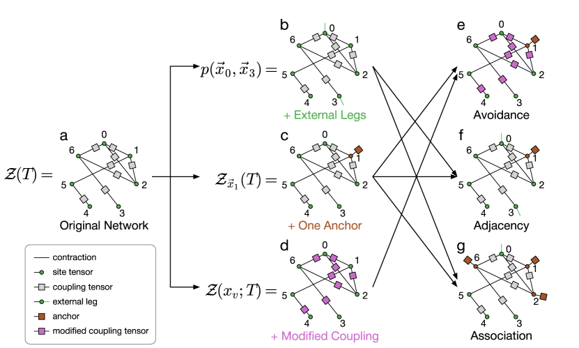
Figure 10: Tensor networks can be used as information structures as combinations of basic moves express complex questions about the design space. Panel (a) shows the original network, panels (b-d) describe the three basic moves that modify its topology, panels (e-g) show how the elementary moves are recombined to study the emergent patterns. (bottom-left corner) Legend of tensor network elements. (a) The original network connects $n=7$ site tensors (green circles) with coupling tensors (gray squares) in the same pattern as the Logical Architecture (Fig. 2 top). Since this network has no outgoing legs, it contracts into a single scalar number equal to the partition function $\mathcal{Z}(T)$. (b) Move 1 adds extra outgoing legs on site tensors 0 and 3 (green lines), making the contraction result in the rank-2 tensor containing the joint marginal probability distribution on the spatial positions of the two units $p(\vec{x}_{0},\vec{x}_{3})$. (d) Move 2 attaches an additional rank-1 anchor tensor (brown square) to site 1, fixing it to a specific spatial location. This network contracts to the conditional partition function $\mathcal{Z}_{\vec{x}_{1}}$. (d) Move 3 modifies all of the coupling tensors (shown as pink squares), for example to account for the voids. This network contracts to the modified partition function $\mathcal{Z}(x_{v};T)$. (e) For the avoidance pattern, we use both anchors and modified couplings to compute the placement opportunity cost via Eqn. 6. (f) For the adjacency pattern, we fix node 1 with an anchor and compute the 2-unit marginal distributions $p(\vec{x}_{i},\vec{x}_{j})$ for all possible pairs of external legs $i,j$, and further convert them into bond order diagrams. (g) For the association pattern, we encode the past design decisions with anchors on units 1, 2, 6 and study the 1-unit marginal distributions on each of the other units.

The partition function of the system can be expressed in terms of the effective design objective in the following factorized form:

$$\mathcal{Z}(T)=\sum\limits_{\{\vec{x}\}}\prod\limits_{\begin{subarray}{c}i<j:\\ A_{ij}\neq 0\end{subarray}}e^{-f(\vec{x}_{i},\vec{x}_{j};T)}.$$ (9)

We interpret the factorized partition function (9) graphically in the form of a tensor network (Fig. 10a). Like other networks, a tensor network consists of nodes and links. Each node is a tensor with rank equal to node degree, and the network links represent the pattern of tensor contractions. We construct tensor networks following a recent prescription of Ref. Jermyn (2020), in which the tensor networks are bipartite: they consist of coupling tensors and site tensors, with each type only connected to the other type as shown in Fig. 10a. Logical architecture $A_{ij}$ is contained in the pattern of the coupling tensors, whereas physical architecture domain $\{\vec{x}\}$ serves as the index of all the tensors, and the design objective determines the contents of the tensors.

The basic tensor network (Fig. 10a) represents the partition function $\mathcal{Z}(T)$ and is merely an alternative, graphical way to express Eq. 9. Each multiplicative term in the partition function becomes a rank-2 coupling tensor with elements defined as $M_{\vec{x}_{i}\vec{x}_{j}}\equiv e^{f(\vec{x}_{i}\vec{x}_{j};T)}$ (note elementwise rather than matrix exponentiation). The site tensors have the form of a multi-dimensional Kronecker delta with the rank corresponding to site’s degree in the logical network $A_{ij}$. For example, the unit 0 in Fig. 10a has three network neighbors, and thus corresponds to a rank-3 tensor $\delta_{\vec{x}_{01}\vec{x}_{02}\vec{x}_{06}}$. The indices mean the value of unit 0 coordinate $\vec{x}_{0}$ that is “presented” to each network neighbor, in this case units 1, 2, and 6. The Kronecker delta ensures that each neighbor perceives the unit 0 at the same location, while index summation ensures that all possible locations are considered. The rank of site tensors can be adjusted for other computations, as shown below. For brevity of notation, we suppress indices on edges because the contraction pattern is dictated by the graphical notation.

Contracting all the tensors along the network links corresponds to performing the sum in Eq. 9. Since that sum has no free indices, the network of Fig. 10a has no external (unpaired) legs. Contraction of the network preserves the number of external legs, resulting in a rank-0 tensor, a scalar number. Since each coupling tensor implicitly depends on cost tolerance $T$, the result of contraction is the $T$-dependent partition function $\mathcal{Z}(T)$.

In order to compute quantities other than the partition function, we add minor modifications of the tensor network. These modifications are described in the graphical language of moves. Here we define three moves: adding external legs, adding anchors, and modifying the coupling tensors (Fig. 10b-d). These moves are recombined to create networks that address the patterns of avoidance, adjacency, and association (Fig. 10e-g).

A.2 Move 1: External Legs

The first move adds extra legs to specific site tensors to control whether specific design degrees of freedom are marginalized or not. If none of the degrees of freedom are marginalized, then carrying out the multiplication but not the summation in the sum (9) would result in an un-normalized joint probability distribution $p(\{\vec{x}_{i}\})$ over all the units, which is a rank-$N$ tensor of prohibitive size. However, following the usual probability theory calculus, in a joint probability distribution each of the entering variables can be in three states: joint, marginalized, or conditional. In the tensor network representation of Fig. 10a, every variable $\vec{x}_{0},\vec{x}_{1},\dots$ is marginalized, resulting in the distribution normalization, i.e. the partition function $\mathcal{Z}(T)$.

In this perspective, a special action needs to be taken to not marginalize some of the variables. We do this by adding external legs to the corresponding site tensors (green lines in Fig. 10b). External legs are the site degrees of freedom that are not summed over, functioning as free indices for the sum (9). The result of contracting the network in Fig. 10b is a rank-2 tensor that represents the un-normalized joint probability distribution $p(\vec{x}_{0},\vec{x}_{3})$. Since the original network contracted to yield the full $\mathcal{Z}$, the normalized probability distribution can be expressed as $\tilde{p}=p/\mathcal{Z}$.

A.3 Move 2: Anchors

The second move adds anchor tensors to the network. The anchors represent the design decisions already taken and woven into the information structure, thus encoding the brownfield aspects of design. In tensor network language, this is equivalent to fixing some of the local degrees of freedom $\vec{x}_{i}$ and thus summing over a restricted ensemble, conditional on the fixed $\vec{x}_{i}$. We do this by creating an additional tensor that we call an “anchor”. An anchor is a rank-1 tensor (vector) that is coupled to a site tensor and is illustrated as purple square in Fig. 10c. The elements of an anchor vector are given by the Kronecker delta $\delta(\vec{x}_{i},\vec{x}_{a})$, where $\vec{x}_{i}$ is the index connected to the site and $\vec{x}_{a}$ is the specific location to which the functional unit is pinned as result of a design decision. Since we didn’t create any external legs, the tensor network in Fig. 10c also contracts to a scalar number of conditional partition function $\mathcal{Z}_{x_{6}}$ that functions as a similar statistical summary of the system as the original partition function $\mathcal{Z}$.

A.4 Move 3: Modified Coupling

The third move modifies the coupling tensors $M(\vec{x}_{i},\vec{x}_{j})$ and traces the effect of this modification on the partition function. In our study, we use the modification to account for the void where no units can be placed. The modification consists of suppressing the statistical weight of the void cells in the coupling tensor:

$$M^{*}(\vec{x}_{i},\vec{x}_{j})=M(\vec{x}_{i},\vec{x}_{j})\prod\limits_{\vec{x}_{v}}(1-\delta(\vec{x}_{i},\vec{x}_{v}))(1-\delta(\vec{x}_{j},\vec{x}_{v})),$$ (10)

where $\vec{x}_{v}$ denotes the positions falling into the excluded void. In the network on Fig. 10d we modified each coupling tensor in this way (marked in pink). The network results in the modified partition function $Z(x_{v};T)$, from which we compute the void free energy via Eq. 6.

A.5 Bond Diagrams

To compute bond diagrams, the raw two-unit distributions $p(\vec{x}_{i},\vec{x}_{j})$ need to be converted into the angular distributions $p_{i\to j}(\theta)$ in post-processing. Since all functional units are placed in a discrete, finite, and fixed set of cells $\vec{x}_{i}$, we pre-compute the directions between any pair of cells $\theta(\vec{x}_{i},\vec{x}_{j})$, measured in radians from $0$ to $2\pi$, ahead of time and store them.

Within the design ensemble, the locations of units $\vec{x}_{i}$ are random, drawn from the joint distribution encoded in the tensor network. We compute a series of marginal two-units distributions $p(\vec{x}_{i},\vec{x}_{j})$ for all pairs $i<j$ (see the tensor network in Fig. 10f). Since the possible unit locations are discrete, the possible directions $\theta(\vec{x}_{i},\vec{x}_{j})$ form an artificially irregular discrete set. This numerical artifact would result in a jagged direction distribution $p_{i\to j}(\theta)$. We smooth the distribution by using a version of non-parameteric Kernel Density Estimation (KDE) Rosenblatt (1956); Parzen (1962) with periodic boundary conditions in which higher angular harmonics are suppressed:

$$p_{i\to j}(\theta)=\frac{1}{\mathcal{N}}\sum\limits_{k}\sum\limits_{\vec{x}_{i},\vec{x}_{j}}p(\vec{x}_{i},\vec{x}_{j})e^{-\frac{1}{2}(hk)^{2}}\cos\left(k(\theta-\theta(\vec{x}_{i},\vec{x}_{j}))\right)$$ (11)

Here $\mathcal{N}$ is a normalization factor, $h$ is the KDE smoothing factor (bandwidth), $k\in\{0,1,2,\dots\}$ is the angular mode index. We find that using smoothing factor of $h=0.1$ radians and angular modes up to $k_{\textsf{max}}=30$ gives good results.

The resulting distributions $p_{i\to j}(\theta)$ need to be compared with the null distribution induced by the Physical Architecture (ship hull shape). We compute the null distribution by evaluating the formula (11) for $p(\vec{x}_{i},\vec{x}_{j})=const$. The identical null distribution is shown in every panel of Fig. 6.

A.6 Numerical Aspects of Computation

Implementing the tensor networks described above on a computer requires two different kinds of computational work: constructing the networks from Logical and Physical Architecture and possible modifications with the three moves, and contracting said networks numerically. We perform these two tasks in Python.

Using code we developed, we create tensor networks by specifying the network topology, the spatial domain geometry, the design objective, and additional moves. These specifications are done via high-level commands, allowing for the rapid generation of diverse networks.

Tensor network contraction is handled by a Python package. Existing tensor network packages use different methods of executing a sequence of pairwise tensor contractions. The contraction result does not depend on the contraction sequence, but the computational time and memory requirements rise by orders of magnitude for suboptimal sequences. Optimal sequences are known for certain frequently used networks, wherease for others one can use exhaustive enumeration algorithms to find the optimal sequence and then execute it repeatedly for the same network topology.Pfeifer et al. (2014) However, almost all networks that we contract in the present work are subtly different, and therefore might require different contraction sequences. We perform all contractions with the PyTNR package, an open-source general purpose tensor network contractor.Jermyn (2020, 2019) The features of PyTNR include using heuristics to automatically generate the contraction sequences on the fly, and performing SVD approximations of controlled precision to reduce the dimension of stored tensors.

The features of PyTNR define the computational constraints on the size of systems that our approach can handle. The size and structure of the Logical Architecture directly change the number of units $n$ in the network and the number of tensors $n_{t}$ (counting both site and coupling tensors). The size or resolution of the Physical Architecture domain directly affect the tensor bond dimension $D$. A rigorous, though pessimistic upper bound on the time complexity of contraction stands at $\mathcal{O}(D^{2\sqrt{\Delta n_{t}}})$, where $\Delta$ is the maximal tensor rank.Kourtis et al. (2019) In contrast, PyTNR relies on a heuristic and stochatic generation of contraction sequences, which complicates even the empirical investigations of numerical scaling of complexity. For highly structured networks, such as $d$-dimensional hypercubic lattices, the time complexity scales a power law $\mathcal{O}(N^{\gamma})$, where the exponent $\gamma$ is a bit larger than the space dimension $d$ and depends on the nature of system’s boundary conditions (periodic or closed).Jermyn (2020)

To provide more concrete numbers, each tensor network contraction in this paper takes less than 10 seconds on a laptop computer (Intel Core i5-3360M @ 2.8GHz CPU, 8Gb RAM) for our example system ($n=7$ units, $n_{t}=15$ tensors, $D=78$, total number of combinatorial states $\mathcal{O}(10^{13})$). The example system size was chosen to best illustrate the physical phenomena at single unit resolution. In other investigations we reliably contracted lattice networks of up to $n_{t}=\mathcal{O}(10^{3})$ tensors accounting for $\mathcal{O}(10^{167})$ combinatorial states using PyTNR.Klishin and van Anders (2020) This result suggests that the current tensor network methods would remain tractable for systems even one order of magnitude larger, or perhaps even larger as the tensor network methods develop.

Appendix B Supplementary Results

B.1 Avoidance: Excess Density

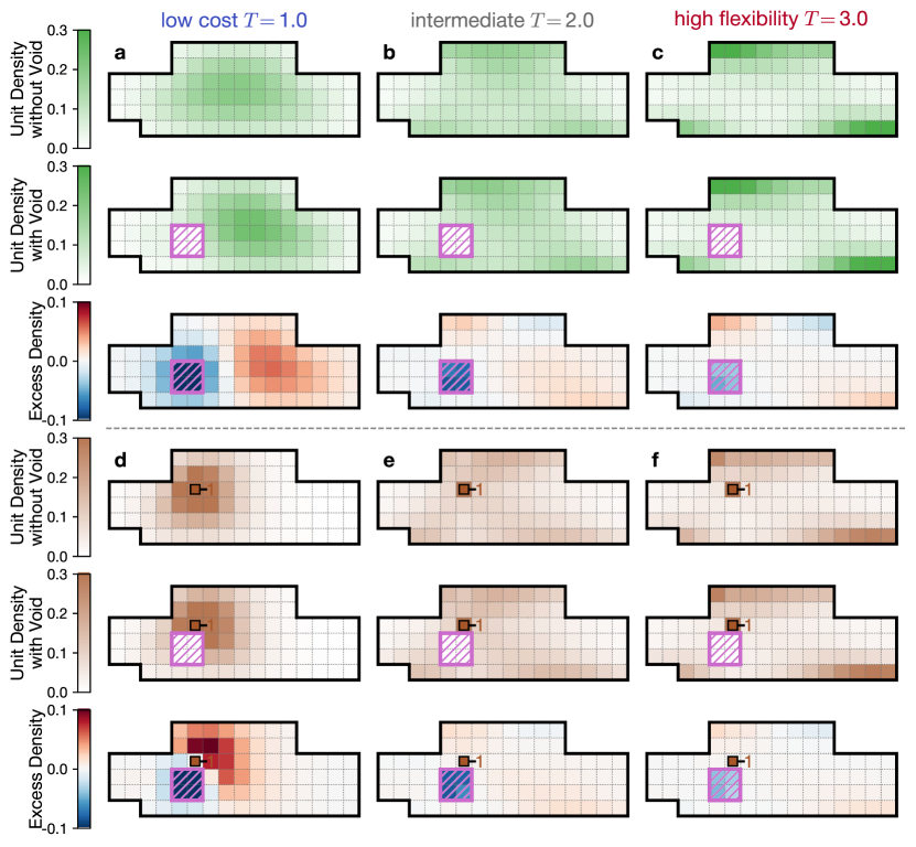
Figure 11: Reserving space in locations with large void premium causes large rearrangements of the unit cloud morphology. The rearrangement is shown via the density profile without the void, with the void, and their pointwise difference (rows) for three values of $T$ (columns, color coded). Panels (a-c) show the rearrangement in a fully greenfield scenario (no anchors). Panels (d-f) show the rearrangement in a brownfield scenario (one anchor indicated with a brown square).

In the main text of the paper we show that void premium quantifies the cost of reserving space within the ship hull, with the effect being further amplified by the presence of an anchor (Figs. 4-5). We associated high void premium with a large rearrangement of the functional units. We can quantify the degree of rearrangement by computing the unit density profile without void $\rho_{\textsf{no void}}(\vec{x})$, the unit density profile with void $\rho_{\textsf{void}}(\vec{x})$, and their difference:

$$\Delta\rho(\vec{x})=\rho_{\textsf{void}}(\vec{x})-\rho_{\textsf{no void}}(\vec{x}),$$ (12)

which we term excess density that can be both positive and negative. Since the total number of functional units does not change upon addition of void, the positive and negative regions of excess density have to cancel each other. In this case large rearrangements of the unit cloud are characterized by large contrast between the positive and negative regions, graphically visible in saturation of colors.

We plot all three densities in Fig. 11, both without and with an anchor on unit 1. In low-cost case $T=1.0$ (panel a) the units want to form a compact cloud, which can be located anywhere within the hull. Upon creation of a void slightly to the left of center, the unit cloud relocates to the right of the void, as seen by large negative $\Delta\rho$ in the left half of the hull and positive in the right half (visible as red and blue clouds). When unit 1 is anchored (panel d), this effect becomes even more pronounced since the unit cloud condenses around a reference point. Creation of a void pushes the unit cloud to the right and above the anchor, but it cannot move far from the anchor, resulting in high contrast of excess density (strong color saturation in the figure) and thus high void premium. At intermediate and high values of $T$, both with and without an anchor (panels b,c,e,f) the rearrangements are much smaller, visible in much paler colors on excess density heatmaps.

B.2 Adjacency: All Bond Diagrams

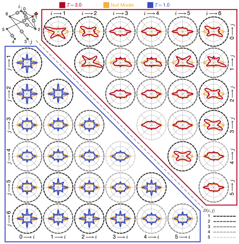
Figure 12: Adjacency patterns between the 7 functional units shown via bond diagrams $p_{i\to j}(\theta)$. (top-left corner) Typical tensor network used for bond diagram computations, with a brown anchor for unit 1 and green external legs at units $i$ and $j$ for each origin-destination pair $i,j$. (bottom-right corner) Legend for the opacity of axes boundaries representing the topological distance $D(i,j)$ varying from 1 to 5 hops. (top-right triangle, red) Bond diagrams for $T=3.0$. (bottom-left triangle, blue) Bond diagrams for $T=1.0$. The origin and destination of each bond diagram are indicated on the outside boundaries of the triangle. Axes in positions symmetric with respects to the diagonal refer to the same origin-destination pair and thus can be directly compared. The yellow curve in each axes shows the null model bond diagram $p_{0}(\theta)$.

In the main text of the paper we show how to compute the bond diagram $p_{i\to j}(\theta)$ for any pair of units $i,j$. Since the directions $\theta(i\to j)$ and $\theta(j\to i)$ only differ by a trivial rotation by angle $\pi$, and the direction from a node to itself is not defined, a system of $n$ units would have $n(n-1)/2$ independent bond diagrams. The Logical Architecture of the example problem was deliberately chosen to not have any graph symmetries, therefore the bond diagrams are not related to each other via any symmetries.

While in the main text we only show several representative bond diagrams (Figs. 6-7), Fig. 12 shows all of the bond diagrams for the low-cost regime $T=1.0$ and the high-flexibility regime $T=3.0$. The diagrams are arranged as a lower-triangular and an upper-triangular matrix of polar plots so that the diagrams in positions symmetric with respect to the diagonal refer to the same pair of functional units and are thus directly comparable. The full set of diagrams shows all adjacency features highlighted in the main text. For units that are directly connected, most of the diagrams at $T=1.0$ show eightfold signal (e.g. 2$\to$6), while diagrams at $T=3.0$ show X-shaped fourfold signal (e.g. 4$\to$5). All diagrams to or from unit 1 show further symmetry breaking because unit 1 is anchored in space. For units that are connected only indirectly with large topological distance, the bond diagram approaches the null model at both $T=1.0$ and $T=3.0$ (e.g. 3$\to$4).

References

- Aikens (1985) C. H. Aikens, European journal of operational research 22, 263 (1985).
- Dorneich and Sahinidis (1995) M. C. Dorneich and N. V. Sahinidis, Engineering Optimization+ A35 25, 131 (1995).
- Drira et al. (2007) A. Drira, H. Pierreval, and S. Hajri-Gabouj, Annual Reviews in Control 31, 255 (2007).
- Owen and Daskin (1998) S. H. Owen and M. S. Daskin, European journal of operational research 111, 423 (1998).
- Shields et al. (2017) C. P. Shields, D. T. Rigterink, and D. J. Singer, Ocean Eng. 135, 236 (2017).
- Dorsey (2003) J. W. Dorsey, Environmental Practice 5, 69 (2003).
- Adams and Watkins (2008) D. Adams and C. Watkins, Greenfields, brownfields and housing development (John Wiley & Sons, 2008).
- Hopkins and Jenkins (2008) R. Hopkins and K. Jenkins, Eating the IT elephant: moving from greenfield development to brownfield (Addison-Wesley Professional, 2008).
- Chalfant (2015) J. Chalfant, Proceedings of the IEEE 103, 2252 (2015).
- Brefort et al. (2018) D. Brefort, C. Shields, A. H. Jansen, E. Duchateau, R. Pawling, K. Droste, T. Jasper, M. Sypniewski, C. Goodrum, M. A. Parsons, M. Y. Kara, M. Roth, D. J. Singer, D. Andrews, H. Hopman, A. Brown, and A. A. Kana, Ocean Eng. 147, 375 (2018).
- Newman (2010) M. Newman, Networks: an introduction (Oxford University Press, 2010).
- Buldyrev et al. (2010) S. V. Buldyrev, R. Parshani, G. Paul, H. E. Stanley, and S. Havlin, Nature 464, 1025 (2010).
- Li et al. (2012) W. Li, A. Bashan, S. V. Buldyrev, H. E. Stanley, and S. Havlin, Phys. Rev. Lett. 108, 228702 (2012).
- Shields et al. (2016) C. P. F. Shields, M. J. Sypniewski, and D. J. Singer, in Proceedings of the 13th International Symposium on PRActical Design of Ships and Other Floating Structures (PRADS’ 2016), edited by U. Nielsen and J. Jensen (Technical University of Denmark, 2016).
- Newman (2003) M. E. Newman, SIAM review 45, 167 (2003).
- Shields and Singer (2017) C. P. Shields and D. J. Singer, Naval Engineers Journal 129, 75 (2017).
- Shields (2017) C. P. F. Shields, Investigating Emergent Design Failures Using a Knowledge-Action-Decision Framework, Ph.D. thesis, University of Michigan (2017).
- Gibbs (1902) J. W. Gibbs, Elementary Principles in Statistical Mechanics (Charles Scribner’s Sons, New York, 1902).
- Klishin et al. (2018a) A. A. Klishin, C. P. Shields, D. J. Singer, and G. van Anders, New J. Phys. 20, 103038 (2018a), arXiv:1709.03388 [physics.soc-ph] .
- Jaynes (1957) E. T. Jaynes, Phys. Rev. 106, 620 (1957).
- Klishin et al. (2018b) A. A. Klishin, A. Kirkley, D. J. Singer, and G. van Anders, (2018b), arXiv:1805.02691 [physics.soc-ph] .
- Penrose (1971) R. Penrose, Combinatorial Mathematics and its Applications 1, 221 (1971).
- Verstraete et al. (2008) F. Verstraete, V. Murg, and J. I. Cirac, Advances in Physics 57, 143 (2008).
- Schollwöck (2011) U. Schollwöck, Annals of Physics 326, 96 (2011).
- Orús (2014) R. Orús, Annals of Physics 349, 117 (2014).
- Chan and Sharma (2011) G. K.-L. Chan and S. Sharma, Annual Review of Physical Chemistry 62, 465 (2011).
- Xie et al. (2009) Z. Xie, H. Jiang, Q. Chen, Z. Weng, and T. Xiang, Phys. Rev. Lett. 103, 160601 (2009).
- Levin and Nave (2007) M. Levin and C. P. Nave, Phys. Rev. Lett. 99, 120601 (2007).
- Biamonte et al. (2015) J. D. Biamonte, J. Morton, and J. Turner, J. Stat. Phys. 160, 1389 (2015).
- Kourtis et al. (2019) S. Kourtis, C. Chamon, E. R. Mucciolo, and A. E. Ruckenstein, SciPost Phys. 7, 060 (2019).
- Cichocki et al. (2016) A. Cichocki, N. Lee, I. Oseledets, A.-H. Phan, Q. Zhao, D. P. Mandic, et al., Foundations and Trends® in Machine Learning 9, 249 (2016).
- Cichocki et al. (2017) A. Cichocki, A.-H. Phan, Q. Zhao, N. Lee, I. Oseledets, M. Sugiyama, D. P. Mandic, et al., Foundations and Trends® in Machine Learning 9, 431 (2017).
- Oseledets (2011) I. V. Oseledets, SIAM Journal on Scientific Computing 33, 2295 (2011).
- Stoudenmire and Schwab (2016) E. Stoudenmire and D. J. Schwab, in Advances in Neural Information Processing Systems (2016) pp. 4799–4807.
- Goldenfeld (1992) N. Goldenfeld, Lectures on phase transitions and the renormalization group (Addison-Wesley, Reading MA, 1992).
- Steinhardt et al. (1983) P. J. Steinhardt, D. R. Nelson, and M. Ronchetti, Physics Review B 28, 784 (1983).
- Roth and Denton (2000) J. Roth and A. R. Denton, Phys. Rev. E 61, 6845 (2000).
- Thouless (1974) D. J. Thouless, Physics Reports 13, 93 (1974).
- Filoche and Mayboroda (2009) M. Filoche and S. Mayboroda, Physical review letters 103, 254301 (2009).
- Jermyn (2020) A. S. Jermyn, SciPost Phys. 8, 5 (2020), arXiv:1709.03080 .
- Rosenblatt (1956) M. Rosenblatt, The Annals of Mathematical Statistics 27, 832 (1956).
- Parzen (1962) E. Parzen, The Annals of Mathematical Statistics 33, 1065 (1962).
- Pfeifer et al. (2014) R. N. Pfeifer, J. Haegeman, and F. Verstraete, Physical Review E 90, 033315 (2014).
- Jermyn (2019) A. S. Jermyn, Journal of Computational Physics 377, 142 (2019).
- Klishin and van Anders (2020) A. A. Klishin and G. van Anders, Soft Matter 16, 6523 (2020).