ALMA observations and modeling of the rotating outflow in Orion Source I

Abstract

We present ²⁹SiO(J=8–7) $\nu$=0, SiS (J=19–18) $\nu$=0, and ²⁸SiO (J=8–7) $\nu$=1 molecular line archive observations made with the Atacama Large Millimeter/Submillimeter Array (ALMA) of the molecular outflow associated with Orion Source I. The observations show velocity asymmetries about the flow axis which are interpreted as outflow rotation. We find that the rotation velocity ($\sim$4–8 km s^-1) decreases with the vertical distance to the disk. In contrast, the cylindrical radius ($\sim$100–300 au), the expansion velocity ($\sim$2–15 km s^-1), and the axial velocity $v_{\rm z}$ ($\sim$-1–10 km s^-1) increase with the vertical distance. The mass estimated of the molecular outflow $\mathrm{M}_{\rm outflow}\sim$0.66–1.3 M_⊙. Given a kinematic time $\sim$130 yr, this implies a mass loss rate $\dot{\mathrm{M}}_{\rm outflow}\sim 5.1-10\times 10^{-3}$ M_⊙ yr^-1. This massive outflow sets important contraints on disk wind models. We compare the observations with a model of a shell produced by the interaction between an anisotropic stellar wind and an Ulrich accretion flow that corresponds to a rotating molecular envelope in collapse. We find that the model cylindrical radii are consistent with the ²⁹SiO(J=8–7) $\nu$=0 data. The expansion velocities and the axial velocities of the model are similar the observed values, except close to the disk ($z\sim\pm$150 au) for the expansion velocity. Nevertheless, the rotation velocities of the model are a factor $\sim$3–10 lower than the observed values. We conclude that the Ulrich flow alone cannot explain the rotation observed and other possibilities should be explored, like the inclusion of the angular momentum of a disk wind.

=1 The Friends of AASTeX Collaboration

1 Introduction

The molecular outflows and the protostellar jets are present in the star formation process and appear to be more powerful and collimated during the earliest phases of young stellar sources (e.g., Bontemps et al. 1996), however, their origin is under debate. Two scenarios are proposed to explain the formation of the molecular outflows. In the first case, several authors (e.g., Pudritz & Norman 1986, Launhardt et al. 2009, and Pech et al. 2012), propose that the molecular outflows are ejected directly from the accretion disk. Other authors suggest (e.g., Shu et al. 1991, Cantó & Raga 1991, and Raga & Cabrit 1993), that the molecular outflows are a mixture between the entrained material with from the molecular cloud and a fast stellar wind.

The magnetocentrifugal mechanism (Blandford & Payne, 1982) is the principal candidate for producing jets and stellar winds (see reviews by Königl & Pudritz 2000 and Shu et al. 2000), in this mechanism, the rotating magnetic field anchored to the star–disk system drives and collimates these winds (Pudritz et al., 2007; Shang et al., 2007). Nevertheless, it is not clear where the magnetic fields are anchored to the disk. The magnetocentrifugal mechanism has two different origins: X-wind (Shu et al. 1994) and disk winds (Pudritz & Norman 1983). In the first model, these winds are launched close to the star, from the radius where the stellar magnetosphere truncates the disk. In the second model, these winds come from a wider range of the radii. Anderson et al. (2003) found a general relation between the poloidal and toroidal velocity components of the magneto-centrifugal winds at large distances and the rotation velocity at the ejection point. Therefore, the observed rotation velocity of the jet could give information about its origin on the disk.

In recent years, evidence of the rotation in protostellar jets and the molecular outflows has been found. For example, the jets HH 211 (Lee et al. 2009) and HH 212 (Lee et al. 2017) present signature of the rotation of a few km s^-1. Molecular outflows with signature of the rotation are: CB 26 (Launhardt et al. 2009), Ori-S6 (Zapata et al., 2010), HH 797 (Pech et al. 2012), DG Tau B (Zapata et al. 2015), Orion Source I (Hirota et al., 2017), HH 212 (Tabone et al., 2017), HH 30 (Louvet et al., 2018), and NGC 1333 IRAS 4C (Zhang et al., 2018).

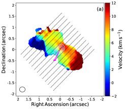
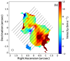
Figure 1: ALMA first moment or the intensity weighted velocity of the emission from the different molecule lines from the outflow. (a) Emission of ²⁹SiO (J=8–7) $\nu$=0. (b) Emission from SiS (J=19–18) $\nu$=0. (c) Emission from ²⁸SiO (J=8–7) $\nu$=1. The diagonal dashed lines indicate the positions where the position-velocity diagrams were made. The color scale bar on the right side shows the $V_{\rm LSR}$ in km s^-1. The synthesized beam of the image is shown in the lower left corner. In these plots the white contours show the continuum emission from the disk and are the 20$\sigma$, 40$\sigma$, 60$\sigma$, and 80$\sigma$. The magenta arrows indicate the proper motion of this source. The size these arrows indicates the proper motions for a period of 100 years. The solid arrows indicate the proper motion and the dashed arrows indicate the proper motion considering the error in right ascension.

Zapata et al. (2015), argued that slow winds ejected from large disk radii do not have enough mass, thus, these winds cannot account for the observed linear and angular momentum rates of the molecular outflow of DG Tau B. Their argument assumed that the mass loss rate of the wind is a small fraction $f\sim 0.1$ of the disk mass accretion rate ($\dot{M}_{w}\sim f\dot{M}_{\rm d,a}$). Nevertheless, recent non-ideal magnetohydrodynamic simulations of magnetized disk winds show that this fraction can be very large, $f\sim 1-2$ (e.g., Bai & Stone 2017; Wang et al. 2019). However, massive disk winds could pose a problem to the disk lifetime. The mass of the disk of DG Tau B is $M_{d}\sim 0.068M_{\odot}$ (Guilloteau et al. 2011). Given the observed outflow mass loss rate $1.7-2.9\times 10^{-7}M_{\odot}{\rm yr}^{-1}$ (de Valon et al. 2020), the disk lifetime is $\tau=M_{d}/\dot{M}_{\rm d,a}=fM_{d}/\dot{M}_{\rm w}\sim f(2-4)\times 10^{5}{\rm\,yr}$. Depending on the value of $f$, the disk lifetime could be smaller than the age of DG Tau B, which has been cataloged as a Class I/II source (Hartmann et al. 2005; Luhman et al. 2010).

The large masses of the molecular outflows can be explained if the outflow is formed mainly by entrained material from the parent cloud. López-Vázquez et al. (2019), hereafter LV19, modeled the molecular outflow as a thin shocked shell, formed by the collision between an anisotropic stellar wind and a rotating molecular cloud in collapse, described by Ulrich (1976). They found that the mass of the molecular outflow, probably, comes from the parent cloud, but the angular momentum could come from both the stellar wind and the parent cloud.

Located at the center of the Kleinmann-Low Nebula in Orion, at a distance $\sim$ 418$\pm$ 6 pc (Kim et al. 2008), the Orion Source I (Orion Src I) is a candidate high mass (M${}_{*}>$ 8 M_⊙) star (Hirota et al. 2014; Plambeck & Wright 2016; Hirota et al. 2017; Ginsburg et al. 2018). The central object of the Orion Src I has a high luminosity $\sim$ 10⁴ L_⊙ (Menten & Reid 1995; Reid et al. 2007; Testi et al. 2010). The bipolar outflow presents low radial velocities ($\sim$ 18 km s^-1) along the northeast-southwest direction, with a size $\sim$ 1000 au (Plambeck et al. 2009; Zapata et al. 2012; Greenhill et al. 2013). This source has a proper motion respect to the nebula center of $\mu_{\alpha}\cos\delta=+2.9\pm 0.4$ mas yr^-1 and $\mu_{\delta}=-5.4\pm 0.4$ mas yr^-1, where the angle $\delta\sim-5^{\circ}$ (Rodríguez et al. 2017). In fact, the Orion Kleinmann-Low Nebula exhibits evidence of a violent explosive phenomenon (e.g., Bally & Zinnecker 2005; Gómez et al. 2008; Zapata et al. 2009; Bally et al. 2017; Zapata et al. 2017). The proper motions of the sources I, BN, and n reveal that this explosion appears to have taken place 500 year ago (e.g., Luhman et al. 2017; Rodríguez et al. 2017).

We present archive ²⁹SiO (J=8–7) $\nu$=0, SiS (J=19–18) $\nu$=0, and ²⁸SiO (J=8–7) $\nu$=1 line observation, made with the Atacama Large Millimeter/Submillimeter Array (ALMA) of the molecular outflow associated with the young star Orion Src I. We also compare the observational results with the thin shell model of LV19. The paper is organized as follows: The Section 2 details the observations. In Section 3 we present our observational results and compare with the outflow model. Finally, the conclusions are presented in Section 4.

Table 1: Molecular lines.

Molecular	Rest
Specie	Frequency
	[GHz]
29SiO(J=8–7) $\nu=0$	342.9808
SiS (J=19–18) $\nu=0$	344.7794
28SiO(J=8–7) $\nu=1$	344.9162

Figure 2: Position-velocity diagrams parallel to the disk mid-plane from the emission of the ²⁹SiO (J=8–7) $\nu$=0 transition at different heights from $z=480$ au to $z=-480$ au with an interval of 80 au. The vertical axes are the line of sight velocity with respect to the LSR velocity and the horizontal axes are the perpendicular distances with respect to the outflow axis. The color scale bar on the right side shows the intensity in Jy/beam.

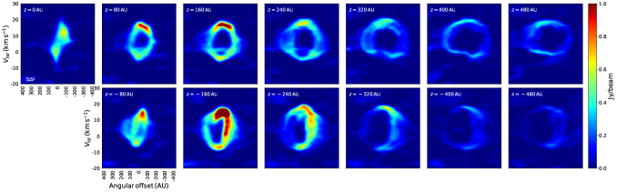
Figure 3: Position-velocity diagrams parallel to the disk mid-plane from the emission of the SiS (J=19–18) $\nu$=0 transition for the same heights and the same description as Figure 2.

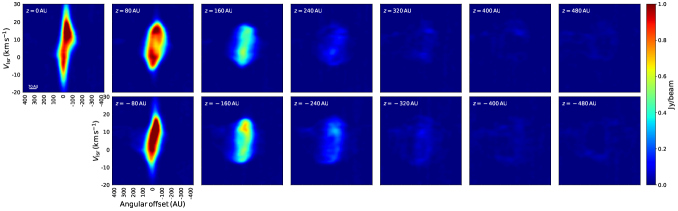
Figure 4: Position-velocity diagrams parallel to the disk mid-plane from the emission of the ²⁸SiO (J=8-7) $\nu$=1 transition for the same heights and the same description as Figure 2.

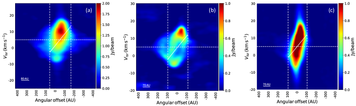
Figure 5: Position-velocity diagrams parallel to the disk midplane at a height $z=-80$ au. (a) Emission from the molecular line of ²⁹SiO (J=8–7) $\nu=0$. (b) Emission from the molecular line SiS (J=19–18) $\nu=0$. (c) Emission from the molecular line of ²⁸SiO (J=8–7) $\nu=1$. The horizontal dashed line shows the value of the LSR velocity of the source. The vertical dashed lines represent the cylindrical radius $\varpi_{\rm obs}$ defined in Figure 6. The solid line in each panel indicates the rotation signature.

2 Observations

The archive observations of Orion Src I were carried out with the Atacama Large Millimeter/Submillimeter Array (ALMA) in band 7 in 2016 October 31st and 2014 July 26th as part of the programs 2016.1.00165.S (P.I. John Bally) and 2012.1.00123.S (P.I. Richard Plambeck), respectively. At that time, the array counted with 31 (2014) and 42 (2016) antennas with a diameter of 12m yielding baselines with projected lengths from 33 to 820 m (41 – 1025 k$\lambda$) and 18 to 1100 m (22 – 1375 k$\lambda$), respectively. The primary beam at this frequency has a full width at half-maximum (FWHM) of about 20^′′, so that in both observations the molecular emission from the outflow of Orion Src I falls well inside of this area.

The integration time on-source was about 25 min., and 32 min. was used for calibration for the 2014 observations, while for the 2016 observations was about 13 min. on-source, and 37 min. for calibration. The ALMA digital correlator was configured with four spectral windows centered at 353.612 GHz (spw0), 355.482 GHz (spw1), 341.493 GHz (spw2), and 343.363 GHz (spw3) with 3840 channels and a space channel of 488.281 kHz or about 0.4 km s^-1 for the 2014 observations and at 344.990 GHz (spw0), 346.990 GHz (spw1), 334.882 GHz (spw2), and 332.990 GHz (spw3) with 1920 channels and a space channel of 976.562 kHz or about 0.8 km s^-1 for the 2016 observations. The spectral lines reported on this study were found in the spw2 (²⁹SiO) of the 2014 observations and the spw0 (SiO and SiS) of the 2016 observations (see Table 1).

For both observations, the weather conditions were reasonably good and stable for these high frequencies. The observations used the quasars: J0510$+$1800, J0522$-$3627, J0527$+$0331, J0532$-$0307, J0607$-$0834, J0423$-$013 and J0541$-$0541 for amplitud, phase, bandpass, pointing, water vapor radiometer, and atmosphere calibration.

The data were calibrated, imaged, and analyzed using the Common Astronomy Software Applications (CASA Version 5.1). The resulting image rms noises for the spectral lines were about 10 mJy Beam^-1 (SiO and SiS) at a angular resolution of 0.19^′′ $\times$ 0.14^′′ with a PA of $-$63^∘ and about 20 mJy Beam^-1 (²⁹SiO) at an angular resolution of 0.30^′′ $\times$ 0.24^′′ with a PA of $+$58^∘. Self-calibration was attempted on the continuum, however, we did not obtain a relatively good improvement in the line maps.

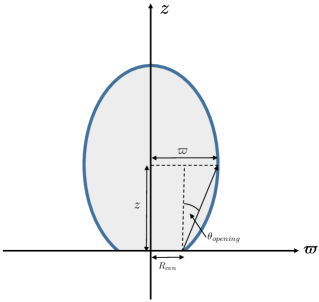
Figure 6: Schematic diagram of a molecular outflow. This diagram shows the opening angle of the molecular outflow $\theta_{\rm opening}$, the cylindrical radius $\varpi$, the centrifugal radius $R_{\rm cen}$, and the height $z$.

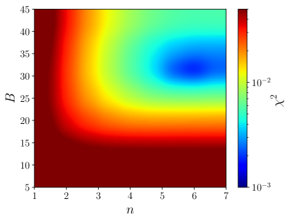
Figure 7: $\chi^{2}$ analysis for different anisotropy parameters $B$ and $n$, with $A=1$, $\alpha=0.1$, $\beta=4$, and an integration time of $t=65$ yr.

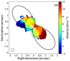
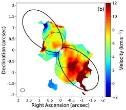
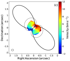
Figure 8: Comparison between the ALMA first moment or the intensity weighted velocity of the emission from the different molecule lines with the best outflow model (see text). (a) Emission of ²⁹SiO (J=8–7) $\nu$=0. (b) Emission from SiS (J=19–18) $\nu$=0. (c) Emission from ²⁸SiO (J=8–7) $\nu$=1. The dashed line represents the isotropic model for parameters $\alpha=0.1$, $\beta=4$, and $B=0$. The solid black line represents the outflow model for the parameters $\alpha$=0.1, $\beta$=4, $r_{s0}(0)=10^{-3}$, $A$=1, $B$=35, and $n$=5.

3 Results and Discussion

Hirota et al. (2017) present observational results with ALMA at 50 au resolution from the emission of the Si¹⁸O and H₂O molecular lines of the molecular outflow of Orion Src I. These lines trace the inner part of the molecular outflow. In contrast, the archive observations used in this work trace the outer part of the molecular outflow, the latter, because this improves an easily comparison with the thin shell model of LV19.

3.1 Results from the observations

Figure 1 presents the first moment or the intensity weighted velocity of the emission from the three molecular lines, ²⁹SiO (J=8–7) $\nu$=0 (panel a), SiS (J=19–18) $\nu$=0 (panel b), and ²⁸SiO (J=8–7) $\nu$=1 (panel c). These panels show that the east side of the molecular outflow presents blueshifted velocities, while the west side presents redshifted velocities. This difference of the velocity is interpreted as rotation around the outflow axis (Hirota et al., 2017). Moreover, Figure 1 indicates that the molecular outflow is not on the plane of the sky, i.e., the outflow has an inclination angle $i\neq 0^{\circ}$: In the lower edge of the outflow (left and middle panels), the molecular outflow has velocities of the order to 12 km s^-1, this high velocity respect to the local standard of the rest velocity $V_{\rm LSR}$ = 5 km s^-1 (Plambeck & Wright 2016), can be explained as the axial velocity. Here, we assume an inclination for the outflow of $i=$10^∘, which is similar to the value reported by Plambeck & Wright (2016), Hirota et al. (2017), and Báez-Rubio et al. (2018). In addition, in the panels (a) and (b), one can observe that the size of the molecular outflow is $\sim$ 1400 au. Finally, the panel (c) show that the molecular line of ²⁸SiO (J=8–7) $\nu$=1 traces the inner most part of the molecular outflow of Orion Src I. Figure 1 also shows the 1.3 mm continuum emission (in white contours) from Orion Src I. This continuum emission is tracing the disk surrounding this source, see Hirota et al. (2017); Plambeck & Wright (2016).

The position-velocity diagrams of the emission from the molecular line of ²⁹SiO (J=8–7) $\nu$=0 are shown in Figure 2. This Figure presents parallel cuts at different distances from the disk mid-plane, these cuts were made from $z$=480 au to $z$=$-$480 au with intervals of 80 au (see the dashed lines in panel (a) of Figure 1). One can observe that in regions near to the disk, this molecule fills the molecular outflow, while, for regions far from the disk, this molecule presents a thin–shell structure in expansion. In addition, one can observe that all position-velocity diagrams present signatures of the rotation (see panel a of Figure 5).

In Figure 3 we have done a similar analysis to Figure 2 for the emission from the molecular line of SiS (J=19–18) $\nu$=0. The position-velocity diagrams show a thin shell structure where the emission from this molecule is very prominent. The width of the shell is $\Delta r\sim$ 120 au which is $\sim$ 1/3 of the distance to the central star. This molecule shows that the outflow is in expansion because the size of the thin shells increases with the distance from the disk. In these diagrams the rotation of the molecular outflow is confirmed. The biggest rotation velocity corresponds to a height of $z=\pm$80 au (see panel b of Figure 5).

Figure 4 shows the position-velocity diagrams of the emission from the molecular line ²⁸SiO (J=8–7) $\nu$=1 for the same distances from the disk mid-plane of the Figures 2 and 3. In contrast to the other two molecules, in this molecular line the thin shell structure does not appear. This Figure confirms the presence of the rotation in the molecular outflow (see panel c of Figure 5). Finally, the absence of the emission for distances of $z\geq\pm$320 au means that this molecule is only tracing the inner part of the molecular outflow. This is maybe due to excitation conditions.

Hirota et al. (2017) measured the rotation velocities for heights between $z=-200$ au and $z=200$ au, and they found that these velocities decrease with the height and have values between $\sim$3–9 km s^-1. In this work, we reported rotation velocities for the same heights of the order of 4–8 km s^-1, these values are similar to those reported by these authors.

Finally, Figure 5 clearly shows the evidence of the rotation and the expansion in Orion Src I. . In this figure, we have made a zoom to the position-velocity diagrams of the Figures 2, 3, and 4 at a distance of $z=-$80 au from the disk for the molecular lines of ²⁹SiO (J=8–7) $\nu$=0 (panel a), SiS (J=19–18) $\nu$=0 (panel b), and ²⁸SiO (J=8–7) $\nu$=1 (panel c), respectively.

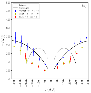
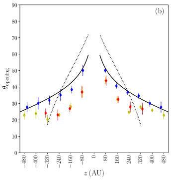
Figure 9: Panel (a) shows the cylindrical radii of the outflow $\varpi$; panel (b) shows the opening angle of the outflow $\theta_{\rm opening}$. These observed values are derived from the position-velocity diagrams in Figures 2, 3, and 4. The error bars are derived from the gaussian fit (see Appendix A for the measurement procedure). The dotted line shows an isotropic model with the parameters $\alpha=0.1$, $\beta=4$, $r_{s0}(0)=10^{-3}$, and $B=0$. The black line shows the best anisotropic stellar wind model with the parameters $\alpha=0.1$, $\beta=4$, $r_{s0}(0)=10^{-3}$, $A=1$, $B=35$, and $n=5$. Both models were integrated up to a dynamical time of 65 yr.

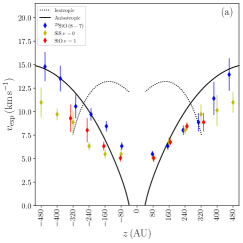
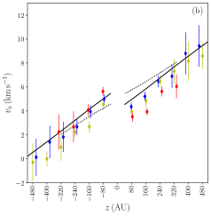
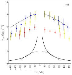
Figure 10: Panel (a) shows the expansion velocity perpendicular to the outflow axis $v_{\rm exp}$ measured at the cylindrical radius; panel (b) shows the axial velocity $v_{\rm z}$; panel (c) shows the rotation velocity $v_{\rm rot}$ measured at the cylindrical radii. These observed values are derived from the position-velocity diagrams in Figures 2, 3, and 4. The error bars are derived from the gaussian fit (see Appendix A for the measurement procedure). The dotted line shows the isotropic model with the parameters of Figure 9. The black line shows the best anisotropic stellar wind model with the parameters of Figure 9. The dashed dotted line of the panel (c) corresponds to the best fitting of the function $v_{\rm rot}=az^{\gamma}+b$ (see text).

3.2 Mass of the outflow

Assuming that the ²⁸SiO (J=8-7) $\nu=1$ emission is optically thick, the excitation temperature is (e.g., Estalella & Anglada 1994)

$$T_{\rm ex}(^{28}{\rm SiO})=\frac{h\nu/k}{\mathrm{ln}\left(1+\frac{h\nu/k}{T_{\rm a}(^{28}{\rm SiO})+J_{\nu}(T_{\rm bg})}\right)},$$ (1)

where $h$ is the Plank constant, $k$ is the Boltzmann constant, $\nu$ is the rest frequency in GHz (see Table 1), $T_{\rm a}(^{28}{\rm SiO})=19$ K is the observed antenna temperature of ²⁸SiO, and $J_{\nu}(T_{\rm bg})$ is intensity in units of temperature at the background temperature $T_{bg}=2.7$ K. Using the value of $\nu$ given in Table 1, we obtain $T_{\rm ex}(^{28}{\rm SiO})=26$ K. Assuming that the ²⁸SiO and ²⁹SiO molecules coexist and share the same excitation temperature, $T_{\rm ex}(^{28}{\rm SiO})=T_{\rm ex}(^{29}{\rm SiO})=T_{\rm ex}$, we can estimate the optical depth of the ²⁹SiO molecule as (e.g., Estalella & Anglada 1994)

$$\tau_{0}(^{29}{\rm SiO})=-{\rm ln}\left[1-\frac{T_{\rm a}(^{29}{\rm SiO})}{J_{\nu}(T_{\rm ex})-J_{\nu}(T_{\rm bg})}\right],$$ (2)

where $T_{\rm a}(^{29}{\rm SiO})=14$ K is the observed antenna temperature of ²⁹SiO and $J_{\nu}(T_{\rm ex})$ is the intensity in units of temperature at the excitation temperature. With these values, we obtain $\tau_{0}(^{29}{\rm SiO})=1.3$, which is not optically thin. Thus, assuming local thermodynamic equilibrium, we calculate the mass of the outflow as a function of the ²⁹SiO optical depth as

$$\frac{\mathrm{M}_{\rm outflow}}{\mathrm{M}_{\odot}} = 5\times 10^{-23}\left(d^{2}\Delta\Omega\right)\left[\frac{m(\mathrm{H_{2}})}{X\left(\frac{{}^{29}{\rm SiO}}{{\rm H}_{2}}\right)}\right]$$ (3)

$$\times \frac{\mathrm{exp}\left[\frac{58.6}{T_{\rm ex}}\right]}{1-\mathrm{exp}\left[\frac{-16.7}{T_{\rm ex}}\right]}T_{\rm ex}\tau_{0}(^{29}{\rm SiO})\Delta v,$$

where $m$(H₂) is the mass of the molecular hydrogen, $\mathrm{X}\left(\frac{{}^{29}{\rm SiO}}{{\rm H}_{2}}\right)=6-12\times 10^{-9}$ is the fractional abundance of ²⁹SiO with respect to H₂. To obtained this value, we assumed a relative abundance of ²⁸SiO with respect to H₂ of $1.2-2.4\times 10^{-7}$, obtained by Ziurys & Friberg (1987) in OMC1 (IRc2), and a relative abundance of ²⁹SiO with respect to ²⁸SiO of 5$\times$10^-2, obtained by Soria-Ruiz et al. (2005) toward evolved stars. The distance $d$ is (418$\pm$6 pc), $\Delta v$ is the velocity width of the line ($\sim$30 km s^-1), and $\Delta\Omega$ is the solid angle of the source ($\sim 1.33\times 10^{-9}$ sr). With these values, the estimated mass of the outflow of Orion Src I is $\rm{M}_{\rm outflow}\gtrsim 0.66-1.3$ M_⊙. This mass is a lower limit because the ²⁸SiO abundance could be lower by up to two orders of magnitude due to the uncertainty in the molecular hydrogen column densities (Ziurys & Friberg 1987).

In addition, for an expansion velocity $v\sim 18\ {\rm km\ s^{-1}}$ (Greenhill et al., 2013) and a size $z=480$ au, the kinematic time is $t_{kin}\sim 130$ yr. Then, the mass loss rate of the molecular outflow as $\dot{\rm M}_{\mathrm{outflow}}=\rm M_{\rm outflow}/t_{kin}\gtrsim 5.1-10\times 10^{-3}$ M_⊙ yr^-1.

Hirota et al. (2017) proposed that molecular outflow of Orion Src I is produced by a slow magnetocentrifugal disk wind. The observed values of the rotational velocities of the outflow can be reproduced by this model which predicts that the wind is eject from footpoints in the disk at radii $r\sim 5-25$ au.

A disk wind requires a very large mass loss rate to account for the mass observed in the outflow. As mentioned in the Introduction, recent MHD simulations show that disk winds around T Tauri stars can have $\dot{M}_{\rm w}=f\dot{M}_{\rm d,a}$, where the fraction can be $f\sim 1-2$ (e.g., Bai & Stone 2017; Béthune et al. 2017; Wang et al. 2019). If the outflow is a disk wind, $\dot{M}_{\rm outflow}=\dot{M}_{\rm w}$. In the case of Orion SrcI, this implies a very large disk accretion rate, $f\dot{M}_{\rm d,a}\gtrsim(5.1-10)\times 10^{-3}M_{\odot}{\rm yr}^{-1}$. Then, massive disk winds face two problems. The first problem has to do with the fact that the mass flux in the disk will eventually fall into the star. Assuming that the disk rotates with Keplerian speed $v_{K}$, the material accreted to the star has to dissipate its energy, $1/2\dot{M}_{\rm d,a}v_{K}^{2}$. Thus, the accretion luminosity at the stellar surface is given by $L_{\rm a}=\eta{GM_{*}\dot{M}_{d,a}\over R_{*}}$, where $G$ is the gravitational constant, $M_{*}$ is the stellar mass, $R_{*}$ is the stellar radius, and $\eta\sim 0.5$. Assuming $M_{*}=15M_{\odot}$ (Ginsburg et al. 2018) and $R_{*}=7.4\,R_{\odot}$ (Testi et al. 2010), the accretion luminosity is $L_{\rm a}\gtrsim(1/f)1.5\times 10^{5}L_{\odot}$. This value is higher than the observed source luminosity $L_{*}\sim 10^{4}L_{\odot}$ (e.g., Menten & Reid 1995; Reid et al. 2007), unless $f\sim 15$. Note that a factor $f\sim 15$ implies that (locally) 94% of the mass the mass escapes into the wind and only 6% accretes towards the star. Disk wind models would have to produce these high $f$ values in the case of winds around massive stars. The second problem, that was already mentioned in the case of DG Tau B (Section 1), is the short disk lifetime. For a maximum disk mass $M_{d}\lesssim M_{*}/3=5M_{\odot}$, necessary for gravitational stability (Shu et al. 1991), and an accretion rate such that $f\dot{M}_{\rm d,a}\gtrsim 5.1-10\times 10^{-3}M_{\odot}{\rm yr}^{-1}$, the disk lifetime is very small, $\tau=M_{d}/\dot{M}_{\rm d,a}\lesssim f\times 980\,{\rm yr}$ (see also the short disk lifetimes in Fig. 33 of Béthune et al. 2017 for disks around low mass stars). This estimate of the disk lifetime assumes that the disk mass is not replenished. Nevertheless, Orion Src I has a massive accreting envelope that could replenish the disk. The disk wind models would have to explore if the disk mass could be replenished in short timescales ($\lesssim 10^{4}$ yr) by the infalling envelope. Both, the accretion luminosity and the disk lifetime, are important constraints on the disk wind models.

Moreover, if there is an accreting envelope around the Orion Src I, a stellar or disk wind will necessarily collide against it, driving a shell of entrained material. For this reason, in this work we explore a model where the molecular outflow is a shell produced by the interaction of a stellar wind and an accretion flow as the scenario first proposed by Snell et al. (1980). The shell is fed by both the stellar wind and the accretion flow. The latter can have very large mass accretion rates as observed in the case of young massive stars (e.g., Zapata et al. 2008; Wu et al. 2009). We will verify under which conditions this shell model can acquire the observed mass.

3.3 Comparison with the outflow model

The position-velocity diagrams, presented in Figures 2-4, show the detailed structure of the outflow velocity as a function of the distance from the disk mid–plane. With these diagrams, we can also obtain information about the kinematic and physical properties of the outflow and compare with the outflow model of LV19.

Goddi et al. (2011) suggested that this source is a binary system with a stellar mass of $\sim$20 M_⊙, and a separation of the stars $<$10 au. Since this separation is very small compared to the size of the outflow, even if each star has its own stellar wind, a single stellar wind emanating from the center is a good approximation.

The proper motion of the Orion Src I with respect to the center of the explosive event that occured 500 yr ago (Rodríguez et al. 2017) will change the environment of the central star. Its envelope will not be a gravitational collapsing envelope of the Ulrich type since the free fall time of a gas parcel starting at an outflow distance $\sim 1000$ au from star is of the order of twice the crossing time. Nevertheless, we will apply the models of LV19 and see how well the observational properties of the outflow can be reproduced.

The model of LV19 assumes that the molecular outflow is a thin shell formed by the collision between a stellar wind and a molecular rotating cloud in gravitational collapse. The thin shell assumption is adequate because the width of the shell is $\Delta r\sim 1/3$ of the distance to central star (see Section 3.1). For our comparison we assume a stellar mass M${}_{*}=15$ M_⊙ (Ginsburg et al. 2018) and a centrifugal radius of $R_{\rm cen}=40$ au, within the range of 21 au - 47 au reported by Hirota et al. 2017.

This model depends of two parameters associated with the properties of the stellar wind and the accretion flow. The first parameter is the ratio between the wind mass loss rate $\dot{\mathrm{M}}_{w}$, and the mass accretion rate of the envelope $\dot{\mathrm{M}}_{a}$

$$\alpha=\frac{\dot{\mathrm{M}}_{w}}{\dot{\mathrm{M}}_{a}},$$ (4)

for this case, we assume a value of $\alpha=0.1$, a typical value the molecular outflows (Ellerbroek et al. 2013; Nisini et al. 2018). The second parameter is the ratio between the stellar wind and the accretion flow momentum rates

$$\beta=\frac{\dot{\mathrm{M}}_{w}v_{w}}{\dot{\mathrm{M}}_{a}v_{0}}=\alpha\frac{v_{w}}{v_{0}},$$ (5)

where $v_{w}$ is the velocity of the stellar wind, and $v_{0}$ is the free fall velocity at the centrifugal radius, given by

$$v_{0}=\left(\frac{\mathrm{GM}_{*}}{R_{\rm cen}}\right)^{1/2}.$$ (6)

For inferred values $\mathrm{M}_{*}=15\,\mathrm{M}_{\odot}$ and $R_{\rm cen}=40$ au, the free fall velocity is $v_{0}=19$ km s^-1. Assuming a stellar wind velocity $\sim 800$ km s^-1, of the order of the escape speed for a star with $R_{*}\sim 7.4R_{\odot}$ (Testi et al. 2010), implies that $\beta\simeq 4$.

We assume a density profile of the stellar wind given by

$$\rho_{w}=\frac{\dot{\mathrm{M}}_{w}}{4\pi r^{2}v_{w}}f\left(\theta\right),$$ (7)

where $f\left(\theta\right)$ is the anisotropy function given by

$$f\left(\theta\right)=\frac{A+B\cos^{2n}\theta}{A+B/(2n+1)}.$$ (8)

The physical properties of the shell model that will be compared with the observations are: the cylindrical radius $\varpi$, the opening angle $\theta_{\rm opening}$, the expansion velocity $v_{\rm exp}$, the axial velocity $v_{z}$, and the rotation velocity $v_{\rm rot}$. Figure 6 presents a schematic diagram of the molecular outflow that shows the cylindrical radius, the height over the disk mid-plane, and the opening angle. The procedure used to measured these quantities is described in Appendix A.

We considered two models: a shell formed by an isotropic stellar wind with $B=0$; and a shell formed by a very anisotropic stellar wind, with $A=1$, $B=35$, and $n=5$. The parameters of the anisotropic stellar wind model are chosen to reproduce the shape of the most extended outflow emission as traced by the ²⁹SiO (J=8–7) $\nu=0$ transition. We choose the parameters that minimize $\chi^{2}$, defined as

$$\chi^{2}=\frac{1}{N}\sum\frac{\left(\varpi_{\rm obs}-\varpi_{\rm model}\right)^{2}}{\varpi_{\rm obs}^{2}},$$ (9)

where $\varpi_{\rm obs}$ is the observed cylindrical radius, $\varpi_{\rm model}$ is the model cylindrical radius, and $N$ is the number of observed values along the $z$ axis. This analysis is shown in Figure 7. We integrate in time the shell model from a small initial shell radius $r_{s0}(0)\simeq R_{*}/R_{\rm cen}\sim 10^{-3}$, close to the stellar surface, until the cylindrical radii of the model $\varpi_{\rm model}$ reaches the observed cylindrical radii $\varpi_{\rm obs}$ at different heights as shown in panel (a) of the Figure 9, which happens at $t=65$ yr. The shell model $R_{s}(\theta)$ is shown in Figure 8. Because the shell decelerates with time, the dynamical time (65 yr) is half of the kinematic time (130 yr) calculated in Section 3.2. Figure 8 shows shell produced by the isotropic wind (dashed line) and the anisotropic stellar wind (solid line) model superimposed on the ALMA first moment of the line emission ²⁹SiO (J=8–7) $\nu$=0 (panel a), SiS (J=19–18) $\nu$=0 (panel b), and ²⁸SiO (J=8–7) $\nu$=1 (panel c).

The comparison between both outflow models with the observational data is shown in Figures 9 and 10. Since the isotropic wind model (dotted lines) does not reproduce the observations, hereafter, we will only discuss the properties of the anisotropic stellar wind model.

The panel (a) of the Figure 9 shows the cylindrical radius obtained from the three line observations and from the anisotropic stellar wind model. These radii are shown as vertical dashed lines in Figure 5. The cylindrical radius $\varpi$ increases with the height above the disk mid-plane, and one can see that the model (black solid lines) agree well with observational data.

For fixed centrifugal radius $R_{\rm cen}$, the opening angle can be defined as

$$\theta_{\rm opening}=\tan^{-1}\left(\frac{\varpi-R_{\rm cen}}{z}\right).$$ (10)

This angle is shown in panel (b) of the Figure 9. The observed values and the model (black solid lines) are consistent. The fact that the opening angle decreases with the height above the disk, indicates that the molecular outflow could close up at higher heights. Nevertheless, one needs observations of a molecule that emits at higher disk heights to establish the outflow shape.

The panel (a) of the Figure 10 shows the expansion velocity for the three molecules indicated in the panel. This velocity increases with the height above the disk mid-plane. The model expansion velocities (black solid lines) are similar to the observed values except close to the disk ($z<\pm 150$ au).

Panel (b) of the Figure 10 shows the measured axial velocity $v_{z}$. This velocity increases with the height above the disk mid–plane. The axial velocity of the anisotropic stellar wind model corrected by the inclination angle $i=10^{\circ}$ and a system velocity $V_{\rm LSR}=5\ {\rm km\,s}^{-1}$ (e.g., Plambeck & Wright 2016) fits the data well.

The rotation velocity is shown in panel (c) of the Figure 10. For the molecular line of ²⁹SiO (J=8–7) $\nu=0$ (blue points), the rotation velocity is in the range 5–8 km s^-1: at $z=\pm$80 au above the disk the rotation velocity is $\sim$8 km s^-1 and it decreases with height. The SiS (J=19–18) $\nu=0$ line (yellow points) has a similar behavior. The ²⁸SiO (J=8–7) $\nu=1$ emission (red points) behaves in the same way but has slightly lower velocities, in the range 4–6 km s^-1. The observed rotation velocity is a factor of 3$-$10 larger than those of the anisotropic stellar wind model. Furthermore, the rotation velocity of the model decreases steeply with the height; the observed rotation velocity slowly decreases. For reference, a polynomial function $(v_{\rm rot}/\rm{kms}^{-1})=a\left(z/{\rm au}\right)^{\gamma}+b$ with $a=-1.5\times 10^{-3}$, $\gamma=1.2$, and $b=8.3$ is shown as a dashed dotted line in panel (c) of Figure 10.

One can also compare the model shell mass with the observed outflow mass (Section 3.2). The shell mass is given by

$$M_{\rm outflow}=\frac{\dot{M}_{\rm a}R_{\rm cen}}{v_{0}}\int_{0}^{\pi/2}p_{m}d\theta,$$ (11)

where $p_{m}$ is the non dimensional mass flux (eq. [47] of LV19). For the anisotropic stellar wind model, $\int_{0}^{\pi/2}p_{m}d\theta=6.0$, in non dimensional units. Therefore, for the values of the centrifugal radius and free fall velocity above, one requires a mass accretion rate of the envelope $\dot{\mathrm{M}}_{a}=1.1-2.2\times 10^{-2}$ M_⊙ yr^-1 to obtain the observed mass of the shell, $M_{\rm outflow}=0.66-1.3M_{\odot}$. Such large mass envelope accretion rates have been inferred in regions of high mass star formation (e.g., Zapata et al. 2008; Wu et al. 2009.) This accretion rate corresponds a mass loss rate of the molecular outflow corrected by the dynamical time $\dot{M}_{\rm outflow}^{\prime}=(0.66-1.3$ M${}_{\odot})/65$ yr = 1 - 2 $\times 10^{-2}$ M_⊙ yr^-1 which is very similar to $\dot{M}_{\rm a}$. Thus, the small fraction of mass that slides along the shell towards the equator does not increase the disk mass significantly.

In summary, the comparison between the anisotropic stellar wind model and the observations of the outflow from Orion Src I fits very well the outflow cylindrical radius. The opening angle is a function of the cylindrical radius, therefore, it also fits the observations well. The expansion velocity and the axial velocity $v_{z}$ have a behavior similar to the observations, although the slope is somewhat different. Nevertheless, the model rotation velocity is much lower (3$-$10 times) than the observed velocity.

The smaller rotation velocity profile of the model indicates that the envelope of Ulrich (1976) can not explain the rotation in molecular outflows. This problem could be alleviated if one includes a stellar wind or disk wind with angular momentum, or increases the angular momentum of the envelope.

For a representative height of $z\sim 240$ au, the observed rotation velocity is a factor $\sim 6$ of the model rotation velocity. Thus, the model has only $\sim 17\%$ of the observed specific angular momentum. The missing angular momentum could come from an accreting envelope with more angular momentum, or from an extended disk wind.

4 Conclusions

In this study, we present new and sensitive ALMA archive observations of the rotating outflow from Orion Src I. In the following, we describe our main results.

• The Orion Src I outflow has a mass loss rate $\dot{M}_{\rm outflow}=5.1-10\times 10^{-3}\,M_{\odot}{\rm yr}^{-1}$. This massive outflow poses stringent constraints on disk wind models concerning the accretion luminosity and the disk lifetime.

• We find that the opening angle (in a range of $\sim$20–60^∘) and the rotation velocity (in a range of $\sim$4–8 km s^-1) decrease with the height to the disk. In contrast, the cylindrical radius (in a range of $\sim$100–300 au), the expansion velocity (in a range of $\sim$2–15 km s^-1), and the axial velocity $v_{\rm z}$ (in a range of $\sim$ -1–10 km s^-1) increase with respect to the height above the disk.

• We compare with the outflow model of LV19, where the molecular outflow corresponds to a shell produced by the interaction of a stellar wind and an accretion flow.

• We find that the observed values of the cylindrical radius, the opening angle, the expansion velocity, and the axial velocity $v_{\rm z}$ show a similar behavior to LV19 anisotropic stellar wind model. However, the rotation velocity of the model is lower (by a factor of 3–10) than the observed rotation velocity of the Orion Src I outflow.

• We conclude that the Ulrich flow alone cannot explain the rotation of the molecular outflow originated from Orion Src I and other possibilities should be explored.

We thank the referee for very useful comments that improved the presentation of the paper. J.A. López-Vázquez and Susana Lizano acknowledge support from PAPIIT–UNAM IN101418 and CONACyT 23863. Luis A. Zapata acknowledges financial support from DGAPA, UNAM, and CONACyT, México. Jorge Cantó acknowledges support from PAPIIT–UNAM–IG 100218. This paper makes use of the following ALMA data: ADS/JAO.ALMA#2016.1.00165.S. and ADS/JAO.ALMA#2012.1.00123.S ALMA is a partnership of ESO (representing its member states), NSF (USA) and NINS (Japan), together with NRC (Canada), MOST and ASIAA (Taiwan), and KASI (Republic of Korea), in cooperation with the Republic of Chile. The Joint ALMA Observatory is operated by ESO, AUI/NRAO and NAOJ. In addition, publications from NA authors must include the standard NRAO acknowledgement: The National Radio Astronomy Observatory is a facility of the National Science Foundation operated under cooperative agreement by Associated Universities, Inc.

Appendix A Measurement procedure

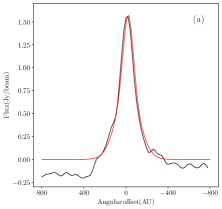
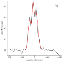
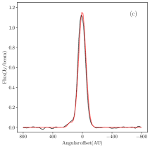
Figure 11: Intensity profiles at $V_{\rm LSR}=5$ km s^-1 of the position-velocity diagrams at a height $z=-80$ au, as indicated by horizontal dashed lines in panels (a)–(c) in Figure 5. The red line shows the best Gaussian fit to the intensity profile of (a) ²⁹SiO (J=8–7) $\nu=0$, (b) SiS (J=19–18) $\nu=0$, and (c) ²⁸SiO (J=8–7) $\nu=1$.

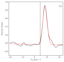
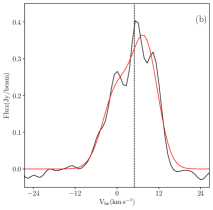
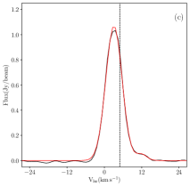
Figure 12: Intensity profiles at the outflow axis of the position-velocity diagrams at a height $z=-80$ au in Figure 5. The red line shows the best Gaussian fit to the intensity profile of (a) ²⁹SiO (J=8–7) $\nu=0$, (b) SiS (J=19–18) $\nu=0$, and (c) ²⁸SiO (J=8–7) $\nu=1$. For reference, the dashed lines indicate the $V_{LSR}$ velocity.

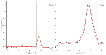
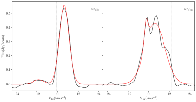
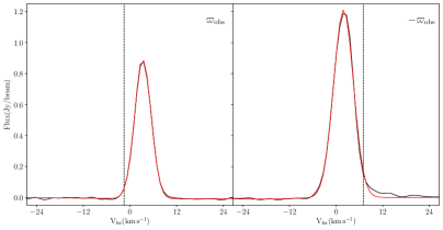
Figure 13: Intensity profiles at the position of the cylindrical radii $\varpi_{\rm obs}$ (left panels) and $-\varpi_{\rm obs}$ (right panels) in Figure 5 at a height $z=-80$ au. The red line shows the best Gaussian fits to the intensity profiles of ²⁹SiO (J=8–7) $\nu=0$ (upper panels), SiS (J=19–18) $\nu=0$ (middle panels), and ²⁸SiO (J=8–7) $\nu=1$ (lower panels).

The position-velocity diagrams in Figures 2–4 were analyzed to derive the physical parameters: the cylindrical radius $\varpi_{\rm obs}$, the expansion velocity $v_{\rm exp}$, and the rotation velocity $v_{\rm rot}$, as a function of the height $z$. These properties were compared with the physical properties of the thin shell model of LV19.

Figure 11 shows the intensity profiles at $V_{\rm LSR}=5$ km s^-1 as a function of the distance to the outflow axis at a height $z=-80$ au for the molecular lines ²⁹SiO (J=8–7) $\nu=0$ (panel a), SiS (J=19–18) $\nu=0$ (panel b), and ²⁸SiO (J=8–7) $\nu=1$ (panel c). These panels also show a Gaussian fit to the intensity profiles (red solid lines). The cylindrical radius $\varpi_{\rm obs}$ is the width of the Gaussian profile and the error if given by the Gaussian fit. In panel (b), the three peaks correspond to the emission from three shells. For our measurements, we only consider the two most prominent peaks. The cylindrical radius of the shell model is the projection of the spherical radius $R_{s}$ at a given height, $\varpi_{\rm model}=R_{s}\sin\theta$, where $\theta=\cos^{-1}(z/R_{s})$.

Figure 12 shows the intensity profiles at a height $z=-80$ au at the outflow axis (angular offset =0 au in Figure 5) as a function of velocity for the three molecular lines, ²⁹SiO (J=8–7) $\nu=0$ (panel a), SiS (J=19–18) $\nu=0$ (panel b), and ²⁸SiO (J=8–7) $\nu=1$ (panel c). The expansion velocity is calculated at the outflow axis as $v_{\rm exp}=(v_{+}-v_{-})/2$, where $v_{\pm}$ are the radial velocities corresponding to the width of the Gaussian profile. The axial velocity $v_{\rm z}$ is calculated as $v_{\rm z}=(v_{+}+v_{-})/2$. The errors are given by the Gaussian fit. In the case of the anisotropic stellar wind model, for a given inclination angle $i$, one calculates $v_{\pm}$ as the projection along the line of sight of the velocity of the two sides of the shell. The axial velocity is also corrected by the system velocity $V_{\rm LSR}$.

Figure 13 shows the intensity profiles as a function of the velocity at the cylindrical radii, $\varpi_{\rm obs}$ (left panels) and $-\varpi_{\rm obs}$ (right panels), shown as vertical dotted lines in Figure 5, for the three molecular lines, ²⁹SiO (J=8–7) $\nu=0$ (upper panels), SiS (J=19–18) $\nu=0$ (middle panels), and ²⁸SiO (J=8–7) $\nu=1$ (lower panels). The red solid lines show the Gaussian fits, some of which require 2 Gaussians.

The rotation velocity is given as the difference between the outer edges of widths of the intensity profiles at $\pm\varpi_{\rm obs}$, indicated by the dashed line in each panel (see also the inclined solid lines in Figure 5). The error bars are given by the Gaussian fit. For the model, we use the rotation velocity $v_{\phi}$.

Figures 11–13 show, as an example, the analysis to obtain the observed quantities $\varpi_{\rm obs}$, $v_{\rm exp}$, $v_{\rm z}$, and $v_{\rm rot}$ at $z=-80$ au. The same analysis is performed for each height $z$ in Figures 9 and 10.

References

- Anderson et al. (2003) Anderson, J. M., Li, Z.-Y., Krasnopolsky, R., & Blandford, R. D. 2003, ApJ, 590, L107
- Báez-Rubio et al. (2018) Báez-Rubio, A., Jiménez-Serra, I., Martín-Pintado, J., et al. 2018, ApJ, 853, 4
- Bai & Stone (2017) Bai, X.-N., & Stone, J. M. 2017, ApJ, 836, 46
- Bally & Zinnecker (2005) Bally, J., & Zinnecker, H. 2005, AJ, 129, 2281
- Bally et al. (2017) Bally, J., Ginsburg, A., Arce, H., et al. 2017, ApJ, 837, 60
- Béthune et al. (2017) Béthune, W., Lesur, G., & Ferreira, J. 2017, A&A, 600, A75
- Blandford & Payne (1982) Blandford, R. D., & Payne, D. G. 1982, MNRAS, 199, 883
- Bontemps et al. (1996) Bontemps, S., Andre, P., Terebey, S., & Cabrit, S. 1996, A&A, 311, 858
- Cantó & Raga (1991) Cantó, J., & Raga, A. C. 1991, ApJ, 372, 646
- de Valon et al. (2020) de Valon, A., Dougados, C., Cabrit, S., et al. 2020, A&A, 634, L12
- Ellerbroek et al. (2013) Ellerbroek, L. E., Podio, L., Kaper, L., et al. 2013, A&A, 551, A5
- Estalella & Anglada (1994) Estalella, R., Anglada, G. 1994, ISBN 84-8338-098-6
- Ginsburg et al. (2018) Ginsburg, A., Bally, J., Goddi, C., Plambeck, R., & Wright, M. 2018, ApJ, 860, 119
- Goddi et al. (2011) Goddi, C., Humphreys, E. M. L., Greenhill, L. J., et al. 2011, The Astrophysical Journal, 728, 15
- Gómez et al. (2008) Gómez, L., Rodríguez, L. F., Loinard, L., et al. 2008, ApJ, 685, 333
- Greenhill et al. (2013) Greenhill, L. J., Goddi, C., Chandler, C. J., Matthews, L. D., & Humphreys, E. M. L. 2013, ApJ, 770, L32
- Guilloteau et al. (2011) Guilloteau, S., Dutrey, A., Piétu, V., et al. 2011, A&A, 529, A105
- Gullbring et al. (1998) Gullbring, E., Hartmann, L., Briceño, C., et al. 1998, ApJ, 492, 323
- Hartmann et al. (2005) Hartmann, L., Megeath, S. T., Allen, L., et al. 2005, ApJ, 629, 881
- Hirota et al. (2014) Hirota, T., Kim, M. K., Kurono, Y., & Honma, M. 2014, ApJ, 782, L28
- Hirota et al. (2017) Hirota, T., Machida, M. N., Matsushita, Y., et al. 2017, Nature Astronomy, 1, 0146
- Kim et al. (2008) Kim, M. K., Hirota, T., Honma, M., et al. 2008, PASJ, 60, 991
- Königl & Pudritz (2000) Königl, A., & Pudritz, R. E. 2000, Protostars and Planets IV, 759
- Launhardt et al. (2009) Launhardt, R., Pavlyuchenkov, Y., Gueth, F., et al. 2009, A&A, 494, 147
- Lee et al. (2009) Lee, C.-F., Hirano, N., Palau, A., et al. 2009, ApJ, 699, 1584
- Lee et al. (2017) Lee, C.-F., Ho, P. T. P., Li, Z.-Y., et al. 2017, Nature Astronomy, 1, 0152
- López-Vázquez et al. (2019) López-Vázquez, J. A., Cantó, J., & Lizano, S. 2019, ApJ, 879, 42
- Louvet et al. (2018) Louvet, F., Dougados, C., Cabrit, S., et al. 2018, A&A, 618, A120
- Luhman et al. (2010) Luhman, K. L., Allen, P. R., Espaillat, C., et al. 2010, ApJS, 186, 111
- Luhman et al. (2017) Luhman, K. L., Robberto, M., Tan, J. C., et al. 2017, ApJ, 838, L3
- Menten & Reid (1995) Menten, K. M., & Reid, M. J. 1995, ApJ, 445, L157
- Nisini et al. (2018) Nisini, B., Antoniucci, S., Alcalá, J. M., et al. 2018, A&A, 609, A87
- Pech et al. (2012) Pech, G., Zapata, L. A., Loinard, L., & Rodríguez, L. F. 2012, ApJ, 751, 78
- Plambeck & Wright (2016) Plambeck, R. L., & Wright, M. C. H. 2016, ApJ, 833, 219
- Plambeck et al. (2009) Plambeck, R. L., Wright, M. C. H., Friedel, D. N., et al. 2009, ApJ, 704, L25
- Pudritz & Norman (1983) Pudritz, R. E., & Norman, C. A. 1983, ApJ, 274, 677
- Pudritz & Norman (1986) Pudritz, R. E., & Norman, C. A. 1986, ApJ, 301, 571
- Pudritz et al. (2007) Pudritz, R. E., Ouyed, R., Fendt, C., & Brandenburg, A. 2007, Protostars and Planets V, 277
- Raga & Cabrit (1993) Raga, A., & Cabrit, S. 1993, A&A, 278, 267
- Reid et al. (2007) Reid, M. J., Menten, K. M., Greenhill, L. J., & Chandler, C. J. 2007, ApJ, 664, 950
- Rodríguez et al. (2017) Rodríguez, L. F., Dzib, S. A., Loinard, L., et al. 2017, The Astrophysical Journal, 834, 140
- Shang et al. (2007) Shang, H., Li, Z.-Y., & Hirano, N. 2007, Protostars and Planets V, 261
- Shu et al. (1994) Shu, F., Najita, J., Ostriker, E., et al. 1994, ApJ, 429, 781
- Shu et al. (2000) Shu, F. H., Najita, J. R., Shang, H., & Li, Z.-Y. 2000, Protostars and Planets IV, 789
- Shu et al. (1991) Shu, F. H., Ruden, S. P., Lada, C. J., & Lizano, S. 1991, ApJ, 370, L31
- Snell et al. (1980) Snell, R. L., Loren, R. B., & Plambeck, R. L. 1980, ApJ, 239, L17
- Soria-Ruiz et al. (2005) Soria-Ruiz, R., Colomer, F., Alcolea, J., et al. 2005, A&A, 432, L39
- Tabone et al. (2017) Tabone, B., Cabrit, S., Bianchi, E., et al. 2017, A&A, 607, L6
- Testi et al. (2010) Testi, L., Tan, J. C., & Palla, F. 2010, A&A, 522, A44
- Ulrich (1976) Ulrich, R. K. 1976, ApJ, 210, 377
- Wang et al. (2019) Wang, L., Bai, X.-N., & Goodman, J. 2019, ApJ, 874, 90
- Wu et al. (2009) Wu, Y., Qin, S.-L., Guan, X., et al. 2009, ApJ, 697, L116
- Zapata et al. (2015) Zapata, L. A., Lizano, S., Rodríguez, L. F., et al. 2015, ApJ, 798, 131
- Zapata et al. (2008) Zapata, L. A., Palau, A., Ho, P. T. P., et al. 2008, A&A, 479, L25
- Zapata et al. (2012) Zapata, L. A., Rodríguez, L. F., Schmid-Burgk, J., et al. 2012, ApJ, 754, L17
- Zapata et al. (2009) Zapata, L. A., Schmid-Burgk, J., Ho, P. T. P., et al. 2009, ApJ, 704, L45
- Zapata et al. (2010) Zapata, L. A., Schmid-Burgk, J., Muders, D., et al. 2010, A&A, 510, A2
- Zapata et al. (2017) Zapata, L. A., Schmid-Burgk, J., Rodríguez, L. F., Palau, A., & Loinard, L. 2017, ApJ, 836, 133
- Zhang et al. (2018) Zhang, Y., Higuchi, A. E., Sakai, N., et al. 2018, ApJ, 864, 76
- Ziurys & Friberg (1987) Ziurys, L. M., & Friberg, P. 1987, ApJ, 314, L49